| Issue |
A&A
Volume 593, September 2016
|
|
|---|---|---|
| Article Number | A72 | |
| Number of page(s) | 11 | |
| Section | Stellar structure and evolution | |
| DOI | https://doi.org/10.1051/0004-6361/201628321 | |
| Published online | 26 September 2016 | |
Do electron-capture supernovae make neutron stars?
First multidimensional hydrodynamic simulations of the oxygen deflagration
1 Heidelberg Institute for Theoretical Studies, Schloss-Wolfsbrunnenweg 35, 69118 Heidelberg, Germany
e-mail: This email address is being protected from spambots. You need JavaScript enabled to view it.
2 Zentrum für Astronomie der Universität Heidelberg, Albert-Ueberle-Str. 2, 69120 Heidelberg, Germany
3 Research School of Astronomy and Astrophysics, Australian National University, Canberra, ACT 2611, Australia
4 ARC Centre of Excellence for All-Sky Astrophysics (CAASTRO), The University of Sydney, NSW 2006, Australia
Received: 16 February 2016
Accepted: 4 July 2016
Abstract
Context. In the classical picture, electron-capture supernovae and the accretion-induced collapse of oxygen-neon white dwarfs undergo an oxygen deflagration phase before gravitational collapse produces a neutron star. These types of core collapse events are postulated to explain several astronomical phenomena. In this work, the oxygen deflagration phase is simulated for the first time using multidimensional hydrodynamics.
Aims. By simulating the oxygen deflagration with multidimensional hydrodynamics and a level-set-based flame approach, new insights can be gained into the explosive deaths of 8−10 M⊙ stars and oxygen-neon white dwarfs that accrete material from a binary companion star. The main aim is to determine whether these events are thermonuclear or core-collapse supernova explosions, and hence whether neutron stars are formed by such phenomena.
Methods. The oxygen deflagration is simulated in oxygen-neon cores with three different central ignition densities. The intermediate density case is perhaps the most realistic, being based on recent nuclear physics calculations and 1D stellar models. The 3D hydrodynamic simulations presented in this work begin from a centrally confined flame structure using a level-set-based flame approach and are performed in 2563 and 5123 numerical resolutions.
Results. In the simulations with intermediate and low ignition density, the cores do not appear to collapse into neutron stars. Instead, almost a solar mass of material becomes unbound from the cores, leaving bound remnants. These simulations represent the case in which semiconvective mixing during the electron-capture phase preceding the deflagration is inefficient. The masses of the bound remnants double when Coulomb corrections are included in the equation of state, however they still do not exceed the effective Chandrasekhar mass and, hence, would not collapse into neutron stars. The simulations with the highest ignition density (log 10ρc = 10.3), representing the case where semiconvective mixing is very efficient, show clear signs that the core will collapse into a neutron star.
Key words: stars: evolution / stars: interiors / stars: neutron / supernovae: general
Alexander von Humboldt Fellow.
© ESO, 2016
1. Introduction
Electron-capture supernovae (ECSNe) and the accretion-induced collapse of oxygen-neon (ONe) white dwarfs (WDs) are phenomena in which a degenerate ONe core is postulated to collapse into a neutron star (Miyaji et al. 1980; Nomoto 1984, 1987; Nomoto & Kondo 1991; Kitaura et al. 2006; Fischer et al. 2010; Jones et al. 2013; Takahashi et al. 2013; Schwab et al. 2015). In the former case, if the SN is from a single star, a type IIP or IIn-P supernova would be produced with a luminosity lower than (Smith 2013) or similar to (Tominaga et al. 2013; Moriya et al. 2014) standard type IIP SNe. It is likely that the progenitor stars of ECSNe have a binary companion (Sana et al. 2012; Dunstall et al. 2015), making it also possible for ECSNe to produce SNe of type Ib/c, depending upon the degree of stripping by the companion star (Tauris et al. 2013).
The collapse of the ONe core is triggered by electron captures on 24Mg and, more importantly, 20Ne, which releases enough energy through the γ-decay of 20O to ignite O-burning via 16O + 16O fusion (Miyaji et al. 1980; Nomoto 1984, 1987). Consequently, and owing to the high degree of degeneracy of the material, a thermonuclear runaway ensues since there is little to no expansion resulting from the temperature increase. Instead, the increase in temperature just accelerates the rate of fusion until the temperature becomes so high (approximately 1010 K) that the composition can be said to be in nuclear statistical equilibrium (NSE; e.g. Seitenzahl et al. 2009). At such temperatures the material is no longer completely degenerate and can expand in response to the nuclear binding energy that has been released at the burning front.
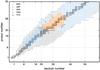 |
Fig. 1 Sources of electron-capture rates considered for the calculation of dYe/ dt in the NSE ashes of the O deflagration. The inverse (β-decay) rates were taken from consistent sources. The labels are as follows: Nabi & Klapdor-Kleingrothaus (2004, NKK), Langanke & Martínez-Pinedo (2001, LMP), Oda et al. (1994, ODA) and Fuller et al. (1985, FFN). ANA corresponds to nuclei for which there are no tabulated rates available and thus we use an analytical formula similar to that used by Arcones et al. (2010) and Sullivan et al. (2016). |
The conservation laws of hydrodynamics allow for two distinct modes of the propagation of combustion fronts, if modelled as discontinuities between fuel and ash: a subsonic deflagration where the flame is mediated by thermal conduction and a supersonic detonation driven by shock waves. Subsonic burning fronts are subject to a variety of hydrodynamical instabilities and produce turbulence. The interaction with turbulent eddies increases the flame surface area and accelerates the flame propagation significantly (see Röpke & Schmidt 2009, for a review). The deflagration model of combustion is the one most commonly assumed to describe the nuclear burning resulting from electron capture by 20Ne and the ignition of 16O fusion in degenerate ONe cores, and in the present work this assumption is held. Assuming that the front propagates as a deflagration, at the high densities in the ONe core the flame width is of sub-centimetre order (Timmes & Woosley 1992) and propagates either by electron conduction (laminar regime) or, if the flame enters the turbulent burning regime, by turbulence.
Models of stars that develop degenerate ONe cores – the so-called super-AGB stars (see, e.g., Siess 2007, 2010) – are riddled with uncertainties, primarily concerning mass loss (Poelarends et al. 2008) and convective boundary mixing (Denissenkov et al. 2013; Jones et al. 2016). If super-AGB stars eject their envelope quiescently by winds or in a dynamical event (e.g., Lau et al. 2012) before the ONe core can grow to the Chandrasekhar mass MCh then an ONe WD and planetary nebula will be formed. It is still possible that the ONe WD will reach MCh by mass accretion from a binary companion. If this occurs and the material is retained by the WD, an O deflagration is ignited owing to electron captures on 20Ne, the interior evolution proceeds in much the same way as is described above for ECSNe (e.g., Schwab et al. 2015) and the star is thought to collapse into a neutron star (Nomoto & Kondo 1991). This is known as accretion-induced collapse (AIC).
The ignition density of the O deflagration has been known to be in the region of 1010 g cm-3 for decades (Miyaji et al. 1980; Nomoto 1987), although its precise value is still a topic of much discussion. Several studies involving the improvement of weak reaction rates for sd-shell nuclei have been undertaken (Takahara et al. 1989; Toki et al. 2013; Lam et al. 2014; Martínez-Pinedo et al. 2014; Schwab et al. 2015) since the seminal works of Fuller et al. (1980, 1982, 1985) and Oda et al. (1994). Most recently, efforts by Martínez-Pinedo et al. (2014) and Schwab et al. (2015), with an analytic approach to 20Ne electron capture including a potentially crucial second-forbidden transition, predict deflagration ignition densities between about log 10ρ = 9.9 and 9.95.
At such high densities, the NSE ashes deleptonise rapidly (dYe/ dt strongly negative). The rapid removal of the electrons reduces their contribution to the pressure, whose gradient supports the star against its own gravity. The result of removing electrons from a completely degenerate core is contraction. Contraction increases the density and along with it, the electron-capture rates. A runaway process ensues thusly and the core of the star, in the current wisdom (Jones et al. 2013; Takahashi et al. 2013; Schwab et al. 2015), is believed to collapse rapidly to a neutron star (more rapidly than a typical iron-core progenitor), launching a shock wave and producing a dim supernova (Kitaura et al. 2006; Fischer et al. 2010) with a relatively low explosion energy and low Ni ejecta mass.
The promptness of the supernova explosion in this case is caused by the steep density gradient at the edge of the core in the progenitor stars of ECSNe and the AIC of ONe WDs. In this more rapid explosion there is postulated to be less time for asymmetries to develop that would have given the newly-born neutron star a natal kick. This distinction between ECSNe/AIC and more massive Fe-core supernovae has been proposed by Knigge et al. (2011) to be responsible for the observed bimodality in the orbital eccentricities of BeX systems. However, the density profiles of the lowest mass Fe-core collapse progenitor stars are very similar indeed to those of ECSN progenitor stars (Jones et al. 2013; Woosley & Heger 2015).
In reality the outcome of ECSNe and the AIC of ONe WDs is not such a closed case. The star’s fate balances on a knife edge between collapsing into a neutron star or becoming completely unbound by the energy released in the thermonuclear runaway as the deflagration runs through the star. It is a situation in which the ignition density of the deflagration, the growth of the Rayleigh-Taylor (R–T) instability, the speed of the deflagration in both the laminar and turbulent regimes, and both electron capture and β-decay of the NSE composition all play critical roles.
Perhaps the most important works highlighting and addressing some of the questions surrounding the O deflagration phase in ECSNe and the AIC of ONe WDs are Nomoto & Kondo (1991), Isern et al. (1991), Canal et al. (1992) and Timmes & Woosley (1992). Nomoto & Kondo (1991) showed that for an ONe core with a central ignition density of 9.95 × 10⁹ g cm-3, the distinction between core collapse and thermonuclear explosion lay with the speed of the convective or turbulent deflagration wave, for which a time-dependent formulation of mixing length theory (MLT) was used in their 1D models. For the mixing length parameter α = 0.7, which reproduces well the observables of type Ia supernovae when used in carbon deflagration simulations (Nomoto et al. 1984), Nomoto & Kondo found that O deflagration results in core collapse, while for α = 1.0 and 1.4 it results in a thermonuclear explosion (their Fig. 1).
Isern et al. (1991) also reported that if the O deflagration were to enter the turbulent burning regime, it could result in either the complete disruption of the ONe core/WD or in the partial ejection of material, leaving behind a bound remnant composed of O, Ne and Fe-group elements. Isern et al. used the parameterisation suggested by Woosley (1986) for the speed of a turbulent flame as the propagation speed of the O deflagration, with the two free parameters set to the estimates given by Woosley (1986) together with the formula. An update to this work by Canal et al. (1992) used the better-resolved electron-capture rate tables by Takahara et al. (1989) and the Ledoux criterion for convection, finding the ignition density of the deflagration to be lower than previously thought. The authors found that even if the flame were to remain in the laminar burning regime, for such a low ignition density (~8.5 × 10⁹ g cm-3) the star would become completely unbound.
The simulations of Canal et al. (1992) did not include Coulomb corrections to the electron-capture reaction rates, which were later shown by Hashimoto et al. (1993, but see the footnote in that paper with regards to Ramon Canal’s own findings) to bring the ignition density back up to 9 × 10⁹ g cm-3. Later still, Gutierrez et al. (1996) found an ignition density of 9.7 × 10⁹ g cm-3, and although the authors included Coulomb effects in the electron-capture reaction rates, they opted to use rates that were more up-to date (Oda et al. 1994) over those that were better resolved (Takahara et al. 1989), which actually may have resulted in a less accurate calculation owing to the undersampling issues of the Oda et al. (1994) rates for these conditions (illustrated in Fig. 6 of Jones et al. 2013, and Fig. 34 of Paxton et al. 2015). Another difference between the work of Gutierrez et al. (1996) and preceding works was the composition of the ONe core. Where previously 20Ne had been considered the most abundant nuclear species based on the models of Miyaji & Nomoto (1987), Gutierrez et al. assumed an oxygen-dominated composition based on the models of Dominguez et al. (1993). Interestingly, the ignition density found by Canal et al. (1992) is actually in rather good agreement with very recent predictions by Schwab et al. (2015), who used the capture rates of Martínez-Pinedo et al. (2014)including Coulomb effects and also assumed the Ledoux criterion for determining convective stability.
The calculations by Timmes & Woosley (1992) of laminar flame speeds and linear analysis of the growth rate of the R–T instability demonstrates just how marginal the situation really is, motivating multidimensional hydrodynamic simulations of the O deflagration phase. In this paper, we report on the progress of such 3D hydrodynamic simulations of the O deflagration that we have performed. Section 2 is a description of the methodology and in Sect. 3 the results of the simulations are presented. Finally, Sect. 4 is a summary of the present work, including a discussion of the uncertainties.
2. Methodology
Degenerate cores comprised homogeneously of a 65%/35% mix of 16O and 20Ne are prescribed a central density and integrated into a hydrostatic equilibrium configuration. They are assumed to be isothermal, with a temperature of 5 × 10⁵ K. In the evolution preceding the formation of an ONe core with this central density (in particular during C burning, the Urca process phase and electron capture on 24Mg), the electron fraction Ye would have decreased slightly from 0.5 (i.e., all nuclei have N = Z). This is important for correctly evaluating the density, and hence the pressure, during the setup. This is accounted for by assuming a constant Ye = 0.493 for the whole core, whose value is a mass-weighted average of the 8.75 M⊙ progenitor model from Jones et al. (2013), which was computed with the MESA stellar evolution code (Paxton et al. 2011, 2013, 2015). If the 8.8 M⊙ model of Jones et al. (2013) had been considered, in which an episode of off-centre Ne and O shell burning had taken place prior to the ignition of the O deflagration, the average Ye would have been 0.490 due to the production of neutron-rich Si-group nuclei. This is a special case that is in itself interesting for a potentially small fraction of ECSN progenitor stars, although its realisation depends upon the uncertain physics of flame quenching in degenerate cores by convective boundary mixing (Denissenkov et al. 2013; Jones et al. 2014; Farmer et al. 2015; Lecoanet et al. 2016).
2.1. 3D hydrodynamics and the level-set based flame
The O deflagration is followed in 3D using the LEAFS code (Reinecke et al. 2002; Röpke & Hillebrandt 2005), which uses a level-set based prescription of the flame front (Reinecke et al. 1999) together with PPM hydrodynamics (Colella & Woodward 1984) and a bilinear interpolation of the Timmes equation of state (EoS; Timmes & Arnett 1999). The gravitational field is described using a Newtonian potential. Where Coulomb corrections are considered in the EoS it is by the formulation of Potekhin & Chabrier (2000). The computational grid consists of a uniform Cartesian grid that expands to track the evolution of the flame front and is nested within a non-uniform Cartesian grid that is designed to follow the expansion of the whole star (Röpke et al. 2006).
The flame speeds are taken from the fitting formulae of Timmes & Woosley (1992) in the laminar regime. A subgrid model for turbulence by Schmidt et al. (2006) is used to calculate the kinetic energy of the fluid on length scales smaller than are resolvable given a finite numerical resolution. The turbulent velocities from this subgrid model are then used to give the flame speed in the turbulent regime.
The nuclear energy release is determined from tabulated NSE abundances, which require an iterative method in order to solve simultaneously for the temperature and the composition. The NSE abundances are tabulated with the density of the fuel being burned as the independent variable. The tables are produced by iteratively writing the abundance tables from post-processing nuclear network calculations and simulating the deflagration in 2D (the same method as used by Fink et al. 2010, for detonations and Ohlmann et al. 2014, for deflagrations). Thermal neutrino losses are also included in the simulations using the formulae by Itoh et al. (1996), as described in Seitenzahl et al. (2015).
Summary of the 3D O deflagration simulations.
The veracity of the assumption that the burning proceeds as a deflagration, as opposed to a detonation, is an interesting subject. The pure detonation of Chandrasekhar-mass CO WDs was ruled out as the predominant explosion scenario for type Ia SNe because the intermediate-mass elements (IMEs) are underproduced (Arnett et al. 1971). Neither have such explosions been observed: there is always a signature of IMEs in the nebular spectra of type Ia SNe. However, since ECSNe and the AIC of ONe WDs are expected to be much less frequent events and whose observational characteristics are not well known, that their burning mode is a detonation cannot be completely ruled out using the same arguments.
2.2. Initial flame surface structure
The initial flame structure is a critical input of the 3D hydrodynamic simulations. 1D stellar models of the pre-deflagration evolution of ECSN progenitor stars and accreting ONe WDs suggest that the deflagration is ignited at a single point in the centre of the star (Nomoto 1984, 1987; Schwab et al. 2015). It is of course not possible to resolve a point in any geometrical sense, and instead the initial flame shape should be something that is representative of the deflagration once it has moved outwards from the centre by a small distance. From a numerical standpoint, it must have moved out far enough that it is able to be resolved at the resolution of the computational grid. This leads to a degree of speculation with regards to how the flame surface has evolved during the time between its inception and the time at which one can resolve it.
In the simulations presented in this work, the flame surface at the beginning of the simulation is constructed as 300 spherical bubbles non-uniformly distributed within a sphere of radius 50 km with its origin at the centre of the ONe core. This represents the surface of a single flame perturbed with small-scale modes. For the model with initial central density  g cm-3, there is 4.8 × 10⁻⁶M⊙ of fuel inside the initial flame, that is transformed into ash during the first time step. The outcome of these simulations is expected to be sensitive to the initial geometry of the flame (see, e.g., Seitenzahl et al. 2013), however a centrally confined ignition with small, but resolvable, perturbations is a sensible first approach (see the Summary and Conclusions of this work for a brief discussion).
2.3. Deleptonisation of the NSE ashes
It is not only electron capture that is important for the evolution of Ye in the ashes of the flame: β-decay and positron capture rates are also significant under the thermodynamic conditions and timescales experienced during the O deflagration. Thus, it was not possible to use the state-of-the-art e−-capture rates by Juodagalvis et al. (2010, J10; as in Takahashi et al. 2013 that are used in core-collapse supernova simulations. This is because (a) J10 do not provide β-decay rates (which are not significant in core-collapse supernovae) and (b) using inconsistent e−-capture and β-decay rates (e.g. e−-capture rates from J10 and β-decay rates from Langanke & Martínez-Pinedo 2001) would upset the detailed balance and misrepresent the deleptonisation rate in the simulation.
The evolution of Ye is followed using its time derivative Ẏe(ρ,T,Ye), which is interpolated from pre-processed tables with T, ρ and Ye as independent variables. The tables were constructed in a similar manner to Seitenzahl et al. (2009): for each point in the 3-dimensional parameter space of the independent variables the NSE equations are solved (Seitenzahl et al. 2009; Pakmor et al. 2012) and the contribution of each nuclear species to the change in Ye is accounted for by folding its abundance with the relevant weak reaction rates.
The sources of the electron-capture reaction rates that were used are shown in Fig. 1. The β-decay (inverse) rates were taken from the same sources as their electron-capture counterparts, to ensure consistency. For protons, neutrons and pf-shell nuclei the shell model rates of Langanke & Martínez-Pinedo (2001, LMP) were used where available. For the sd-shell, the rates of Oda et al. (1994, ODA) were used (also shell model calculations) where available. Where LMP and ODA rates were not available, the rates from Fuller et al. (1985, FFN) were used. Where rates were still missing, the choice falls back to the QRPA rates of Nabi & Klapdor-Kleingrothaus (2004, NKK). All other rates were computed in a similar manner to the approximations described in Arcones et al. (2010) and Sullivan et al. (2016). The neutrino luminosity ϵν is also computed and tabulated in the same manner as Ẏe and is used as a sink term in the energy equation. This is a valid approximation until the density reaches approximately 1011 g cm-3, where neutrino interactions with matter become non-negligible. Such high densities would be realised only in the case of a core collapse event.
3. Results
A number of simulations were performed in either 2563 or 5123 resolution for three initial ONe core structures with  (G series), 9.95 (J series) and 10.3 (H series). Some of the simulations included the effect of Coulomb corrections in the EoS. A summary of the key simulations is provided in Table 1 along with some diagnostic information.
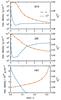 |
Fig. 2 Maximum density and minimum electron fraction Ye in the simulations G14, J02 and H01 (see Table 1). In the G and J simulations ( |


3.1. Outcomes of the simulations
There is a clear distinction between the lower density G and J models and the H models, which had the highest ignition densities. This is shown in Fig. 2, where the maximum density is plotted as a function of time. In the first 5 s, the maximum density in G14 and J02 drops by several orders of magnitude owing to expansion caused by the release of nuclear binding energy. H01, with the highest initial density, on the other hand, experiences only contraction. Within the first few hundred milliseconds the maximum density increases by a factor of 5, reaching almost 1011 g cm-3. At these high densities, the interaction of neutrinos with matter (which is not accounted for in these simulations) should become significant and therefore the simulation could not be continued with the methods and assumptions that were used. The result of the H01 simulation is, however, rather indicative that a core-collapse event will be the fate of such a star. On the other hand, the G and J models – which are based on the current understanding of the 20Ne electron-capture process (Martínez-Pinedo et al. 2014; Schwab et al. 2015) – are a kind of thermonuclear explosion in which a bound ONeFe compact remnant is produced. Although the models by Schwab et al. (2015) include the most accurate treatment of the electron-capture processes, an additional factor in determining the ignition density of the O deflagration in ONe cores is the onset of semiconvection. The dispersion relation for this kind of overstable oscillatory convection was derived by Kato (1966), giving a growth rate of the overstable oscillations. A simplification to the solution of Kato’s equation by Langer et al. (1983, but see also Shibahashi & Osaki 1976 forms the basis of the parameterised diffusion approximation to semiconvective mixing found in many modern stellar evolution codes. Schwab et al. (2015) showed with a timescale argument that Langer’s formulation of semiconvective mixing would likely not (i.e., within the range of typically-used values of the free parameter α) impact upon the ignition density of the O deflagration. Takahashi et al. (2013) on the other hand found an ignition density of ~3 × 10¹⁰ g cm-3 while accounting for semiconvective mixing using the time-dependent mixing formulation described in Unno (1967). This may have been an artefact of the under-resolved tabulations of the 20Ne and 20F electron-capture rates by Oda et al. (1994) used in Takahashi et al. (2013). The importance of semiconvection during the 20Ne electron-capture preceding the thermonuclear runaway is an interesting problem in itself, however it is one that is outside of the scope of the present work. The calculations of Schwab et al. (2015) are taken to be the current standard until further work into the reaction rates or semiconvective instability are undertaken. The simulations performed in this work represent the two extreme cases of semiconvection: in the case of inefficient semiconvection, the G or J series of simulations are the most realistic (depending on the strength of the second forbidden transition from 20Ne to 20F); in the case of semiconvection being so efficient that fully developed convection is established over a short time scale, the H series of simulations would probably be closer to reality.
Another critical quantity in these simulations is the minimum electron fraction  , which is also shown in Fig. 2 (solid blue lines with circular glyphs). In the G14 (J02) model does not go below about 0.40 (0.41), and after a few tens of milliseconds begins to increase again as the density drops and β-decays become more prevalent. As in the case of the maximum density, behaves differently for the H models than for the G and J models: The decrease in pressure caused by the marked reduction in the number of electrons induces a contraction of the ONe core/WD in the H01 simulation which in turn increases the temperature and density, accelerating the rate of deleptonisation in a runaway process. Another important consequence of the reduction in electron fraction and the increase in temperature during the associated contraction is the adjustment of the NSE state. At Ye = 0.3, T = 15 GK and log 10ρ = 10.5 the equilibrium state consists of free neutrons, α particles, intermediate-mass elements and Fe-group elements in roughly equal parts (Fig. 3). The internal energy of such a state is in fact lower than the internal energy of the initial model with O and Ne at T = 5 × 10⁵ K. This, too, results in a gas pressure deficit and favours a core collapse event.
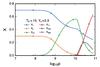 |
Fig. 3 NSE composition as a function of density for the conditions encountered in the simulations with the highest ignition densities (2 × 10¹⁰ g cm-3; T = 1.5 × 10¹⁰ K and Ye = 0.3). Fe denotes elements with Z ≥ 24 and IME the intermediate-mass elements with 13 ≤ Z< 24. The residual is the light elements excluding p, n and α-particles. |
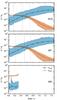 |
Fig. 4 Laminar and turbulent flame speeds as fractions of the sound speed cs (i.e., Mach numbers) during the first 1.5 s of the G13, J01 and H01 simulations (see Table 1). The solid lines show the average (mean) value over the entire burning front. The shaded region extends from the minimum to the maximum speed. The vertical dashed lines demarcate the times at which a) the flame becomes turbulent for the first time; b) the mean turbulent flame speed exceeds the mean laminar flame speed and c) the flame is completely turbulent. In simulation J01 ( |


In about the first 150 ms of the H01 simulation, becomes as low as 0.25 – which was the lower bound of the Ẏe and ϵν tables that were used – and does not decrease any further. Even with the deleptonisation curtailed because of the inadequate domain of the Ẏe tables that had been computed as described in Sect. 2.3, with Ye at the upper limit of 0.25 the model still shows a clear indication of core collapse.
3.2. The bound remnants: ONeFe white dwarfs
A key result of the G and J simulations is that material becomes unbound from the ONe core as a result of the release of nuclear energy during the deflagration, leaving a bound remnant consisting of O and Ne (~60−80%), iron-group elements (~20−40%), and intermediate-mass elements (1−3%). This is in rather good agreement with the 1D calculations of Isern et al. (1991), even though there are some appreciable differences between the approaches of this work and theirs. To summarize: this work uses a more sophisticated EoS, laminar flame speeds from microscopic flame calculations (Timmes & Woosley 1992), modern weak reaction rates, a subgrid model of turbulence and is performed in 4π geometry with 3D hydrodynamics. The mass fractions of O and Ne (0.65 and 0.35, respectively) used in the present work are more representative of the actual composition of the ONe cores, compared to the abundances from Miyaji et al. (1980) that were used by Isern et al. In addition, from the important work of Martínez-Pinedo et al. (2014) and Schwab et al. (2015), the present work benefits from tighter constraints on the ignition density of the deflagration although the value of the ignition density itself has changed little since the work of Isern et al. (1991) and Canal et al. (1992). Despite the significant differences between the present work and that of Isern et al. (1991) and Canal et al. (1992), our qualitative results are in rather good agreement: Isern et al. also found bound WD remnants consisting of a mixture of O, Ne and Fe-group elements. This is really quite a remarkable result.
The mass of the bound remnant is very sensitive to whether or not Coulomb corrections are included in the EoS (see Table 1). Simulations with and without the Coulomb corrections were performed. Including the corrections results in roughly a factor of 2 increase in the mass of the bound remnant and a factor of ~5 decrease in the ejecta mass. These are significant changes and the sensitivity of the quantitative result to the long-range coupling of the ideal components of the plasma being so great motivates further scrutiny of the accuracy with which such Coulomb corrections are treated. The laminar and turbulent flame speeds are shown as a function of time for the 2563 simulations without and with Coulomb corrections to the EoS in Figs. 4 and 5, respectively. One can see that in the simulations where the internal energy – and, hence, the pressure – of the plasma are reduced due to the Coulomb corrections the flame takes longer to become dominated by turbulence. Quite why this seemingly slight shift in the timing of the onset of the turbulent flame results in such a marked decrease in the amount of mass that can reach escape velocity is a detailed problem.
The G14 simulation ejected 0.951 M⊙ of material, of which 0.362 M⊙ is composed of Fe-group elements, and leaves a bound remnant of 0.438 M⊙. The bound remnant consists of 0.115 M⊙ of Fe-group elements with the remaining mass comprised of a mixture of O and Ne in the same 65%/35% proportions of the initial composition of the ONe core/WD. Comparing the numerical values in Table 1 for models G13 (2563) and G14 (5123) it is clear that the quantitative answer is not converged on grid refinement. However, there is a clear indication that the result is qualitatively converged. In particular, the simulation at both resolutions results in the partial ejection of the core material, leaving a bound compact remnant. Doubling the number of grid cells in each spatial dimension from 512 to 1024 and hence increasing the computational expense by a factor of 16 (23 more grid cells and a factor of 2 decrease in the Courant number) seems an unnecessary expense at this time.
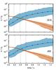 |
Fig. 5 Same as Fig. 4 but for models G15 and J02 ( |
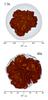 |
Fig. 6 Mass fraction of Fe-group elements in simulation G14 (see Table 1 for details) at 1.3s (top panel) and 60 s (bottom panel) of simulated time. The greyish-blue contour is the surface of the ONe core, which shows a distinct aspherical deformation. Interior to the 0.951 M⊙ of ejecta (which consists of 0.362 M⊙ of Fe-group elements) remains a bound remnant of 0.438 M⊙ consisting of a mixture of O, Ne and 0.115 M⊙ of Fe-group elements. |
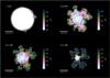 |
Fig. 7 Geometry of the flame surface for different values of the asymmetry diagnostic parameter ζ (1). The plot for ζ = 0 is a snapshot of the H01 simulation at 320 ms of simulated time; the flame surface is essentially a sphere due to the suppression of the Rayleigh-Taylor instability. All of the other plots are of the J01 simulation. The time evolution of ζ is shown in Fig. 8; the asphericity becomes more pronounced with time in the G and J series simulations. Each panel also has a pseudo-colour plot of the electron fraction Ye. |
The J series of models with initial central densities  display similar characteristics and a similar trend to the G series of models with slightly lower ignition density. All of the simulations eject a fraction of the core material and leave a bound remnant with a mass not exceeding the effective Chandrasekhar mass
  . The inclusion of Coulomb corrections to the EoS approximately doubles the mass of the bound remnant, as in the G series. Simulations without Coulomb corrections were not performed in 5123 resolution for the J series however the trend is expected to be the same as in the G series; i.e. the mass of the bound remnant would be lower than in the 2563 simulation.
3.3. A multidimensional problem
A volume rendering of the abundance of Fe-group elements at 60 s of simulated time in the G14 simulation (see Table 1) is shown in Fig. 6. The asymmetry of the deflagration and of the ejecta is striking. This is a result of the growth of the R–T instability. Whether or not the R–T instability is significant in O deflagrations was considered by Timmes & Woosley (1992), who have compared the minimum wavelength instability to the thickness of the density inversion produced by the burning front before it is erased by electron capture (their Fig. 9b). In their case A – which has a ratio of O/Ne that is closest to the core composition in the most recent models of super-AGB stars using the 12C(α,γ)16O rate of Kunz et al. (2002) – the instability grows for ρ ≲ 1.1 × 10¹⁰. This is confirmed by the G14 simulation (and in fact by the entire G and J series of simulations) of the present work, in which the density never exceeds this value (Fig. 2) and indeed R–T plumes can be seen in the Fe-group abundances (Fig. 6). Timmes & Woosley also predicted that for ρ ≳ 1.1 × 10¹⁰, the R–T instability would be suppressed and the core would collapse to form a neutron star. This result is confirmed by the H01 simulation of the present work (see Table 1 and Fig. 2), which results in core collapse. Indeed, the suppression of the R–T instability is observed in the H01 simulation and the flame stays in the laminar regime. The laminar and turbulent flame speeds (see Sect. 2) are shown in Figs. 4 and 5 for the 2563 simulations without and with EoS Coulomb corrections, respectively. The red and blue lines are the mean values of the laminar and turbulent burning speeds, respectively, as Mach numbers over the whole flame surface as a function of time. The shaded regions show the total range of flame speeds over the surface as a function of time. The vertical dashed lines demarcate the times at which (from left to right) the flame becomes turbulent somewhere, the mean turbulent flame speed is higher than the mean laminar flame speed, and the flame is turbulent everywhere. These times are delayed slightly for higher ignition density (compare, e.g., G13 and J01 or G15 and J02). Interestingly, when Coulomb corrections are included in the EoS the flame takes slightly longer to become turbulent anywhere on its surface, but less time is needed for its speed to become completely dominated by turbulence (compare G13 and G15 or J01 and J02).
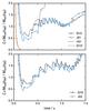 |
Fig. 8 Time evolution of the flame asymmetry diagnostic parameter ζ for 2563 simulations from the G, J and H simulation series (see Table 1). The bottom panel shows the simulations with EoS Coulomb corrections, and the top panel shows the simulations without. The asymmetry develops in much the same way regardless of the inclusion of Coulomb corrections in the EoS, and is even slightly more pronounced when they are included. Clearly, the Rayleigh-Taylor instability is suppressed in the highest density simulation (H01) and the flame surface becomes essentially a sphere (ζ = 0). Figure 7 shows the severity of the asymmetry for different values of ζ, which is difficult to imagine a priori. |
Understanding the impact of the R–T instability on the quantitative results and qualitative outcome of the O deflagration in a differential sense is a difficult – if not impossible – task, because the instability and its growth are the direct result of solving the Euler equations, which is at the very heart of multidimensional hydrodynamic simulations. However, we have defined an instructive flame asymmetry diagnostic parameter  (1)which proves to be a rather robust metric that facilitates a quantitative comparison of the degree of asymmetry of the flame surface resulting from the growth or suppression of the R–T instability due to the relative buoyancy of the ash to the fuel. In Eq. (1), r90 is the radius of the sphere containing 90% of the ashes in the simulation by mass1. Mfuel(r90) is then the mass of fuel (material unburned by the deflagration) inside the radius r90 and similarly Mash is the mass of ash inside that radius. A value of ζ = 0 means that the flame surface is essentially a perfect sphere, as one would find in a 1D representation (e.g., Nomoto & Kondo 1991; Isern et al. 1991; Canal et al. 1992). The degree of asymmetry corresponding to the magnitude of ζ when ζ> 0 (i.e., anything other than a sphere) is difficult to imagine and so in Fig. 7 plots of the flame surface for values of ζ = 0, 0.46, 1.02 and 1.39 are shown, that are realised in the simulations. Since ζ becomes zero only in the simulations with highest ignition density (H series), the corresponding flame surface in Fig. 7 (top left panel) is taken from the H01 simulation. All other panels of Fig. 7 are from the J01 simulation, for consistency. At a value of ζ = 0.46 (top right panel) the flame surface already shows significant deviations from spherical symmetry. Therefore, Fig. 7 serves as useful evidence that for ζ ≳ 0.46 a spherically symmetric flame geometry would be a rather poor approximation. Even a value of ζ = 0.1 (not shown here) to the eye looks distinctly non-spherical. To put this into context, a comparison of the flame asymmetry diagnostic parameter ζ for the three different ignition densities as a function of time during the first 1.5 s (at which time nuclear burning has ceased) is shown in Fig. 8. The bottom panel shows 2563 simulations that include EoS Coulomb corrections and the top panel those without. In both cases the G and J series of simulations exhibit gross deviations from spherical symmetry, while in the high density H01 simulation the flame surface quickly becomes a sphere and remains as such.
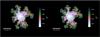 |
Fig. 9 Pseudo-color plot of the electron fraction, Ye, in a slice through the x-y plane in two simulations at 500 ms of simulated time. The right panel is the simulation G13 from Table 1 and the left panel is the same simulation with the turbulent burning speed set to zero, so that the flame may only propagate conductively. The Rayleigh-Taylor fingers are clearly visible in both cases. This shows that large-scale deviations from spherical symmetry during the deflagration are not the result of turbulent burning. The simulations look very similar indeed at this time: the mean turbulent flame speed does not exceed the mean laminar flame speed in G13 until 460 ms (see Fig. 4). |
If the flame had not become turbulent in the G and J series of models, and instead had remained laminar (which is certainly only a hypothetical case), the large-wavelength modes of the R–T instability that can be captured in 3D would still develop. This is shown in Fig. 8, where the line labelled G13′ is the parameter ζ for a simulation that is the same as G13 but with the turbulent flame speed set to zero, so that the flame may only propagate via conduction. It behaves almost identically to G13 until around 0.5 s in that the flame surface becomes more asymmetric over time. This is to be expected since the flame remains on average in the laminar regime until about this time (as is shown in Fig. 4, top panel). In Fig. 9 the electron fraction and flame surface in the G13 simulation with only laminar flame speeds included (left panel) and with both laminar and turbulent flame speeds included (right panel) are plotted at 500 ms. The snapshots do indeed look rather similar. The reason the asymmetry parameter ζ for G13′ rapidly increases after about 0.5 s is that the material has expanded to densities below which the conductive deflagration speeds have been calculated by Timmes & Woosley (1992). The flame speed decreases (as the red line in the top panel of Fig. 4) and, hence, so does the rate of ash production. The ashes are still moved out to larger radii by advection and expansion, however, resulting in a rapid increase in ζ.
Capturing the asphericity of the flame and the ashes using multidimensional simulation techniques appears to be an integral part of studying electron-capture supernovae. It may be possible to reproduce some, but certainly not all, of the global characteristics of the simulations in this work using one-dimensional methods with appropriately parameterised spherical flame models. However, this would have to be proven and performing such 1D simulations is beyond the scope of this work. In any case, the best-suited parameters could almost certainly not be known a priori.
4. Summary and conclusions
3D simulations of the O deflagration phase of ECSN progenitors and the AIC of ONe WDs have been performed in 4π geometry. For ignition densities that we consider to be representative in the light of recent updates to the 20Ne electron-capture rate (Martínez-Pinedo et al. 2014; Schwab et al. 2015), collapse into a neutron star does not occur. Instead, a thermonuclear explosion ejects a portion of the degenerate core/WD, leaving behind a bound remnant consisting of O, Ne and Fe-group elements, confirming the 1D simulations of Isern et al. (1991). What such an event would look like is certainly an interesting question, and one that future work should attempt to address. The recent simulations by Schwab et al. (2015) are based on up-to-date nuclear physics input. We therefore consider our low and intermediate ignition density simulations as reference cases. Note, however, that Schwab et al. (2015) report these to be lower limits. This is because of both the uncertain contribution of the second forbidden transition to the electron-capture rate of 20Ne (as discussed by Schwab et al.) and the uncertain impact of semi-convection.
Since the outcome of these deflagrations are known to be very sensitive to the ignition density (e.g. Nomoto & Kondo 1991; Isern et al. 1991; Canal et al. 1992), simulations with rather high ignition density (2 × 10¹⁰ g cm-3) were also computed. These simulations show clear signs of core collapse, reaching a maximum density of 1011 g cm-3 within 400 ms of the deflagration being ignited. Such a high density ignition may only be realised if significant energy transport by convective motions takes place during the evolution immediately preceding the thermonuclear runaway (Mochkovitch 1984; Miyaji & Nomoto 1987; Gutierrez et al. 1996), although convection is likely suppressed because of the stabilising gradient of mean molecular weight produced during the electron-capture process (Schwab et al. 2015). In the case that semiconvection during the 20Ne electron-capture phase is efficient enough to destroy the gradient in mean molecular weight produced by the electron captures the result will be fully-developed convection. This is likely not the case, however until a more rigorous examination is performed, the contribution of semiconvective mixing to the ignition density remains unclear. It was not possible to follow the collapse of the core any further in the highest density (H-series) models that reach such high densities owing to the limitations of the EoS that was used and the omission of neutrino interactions with matter from the present work.
It is also of course possible that updates to the microphysics in the G and J series models could result in core collapse. Indeed, the uncertainties in the results of the simulations presented in this work are of course a product of the uncertainties in the choice of input physics assumptions and those introduced by the numerical implementation. An example worth highlighting is the ignition geometry (see Sect. 2.2). In the present work a centrally confined ignition was assumed, with small perturbations from which the Rayleigh–Taylor instability can grow, should the time scales allow. The perturbations were large enough to be able to be resolved on the computational grid, so that any test of the sensitivity to numerical resolution study makes sense. Even with these perturbations, cases where the R–T instability could grow (G and J series) and cases where it was suppressed (H series) were clearly distinguishable. It is quite difficult to imagine that the flame would propagate outwards from a single central ignition point as a perfect sphere, but that does not mean the magnitude of the perturbations used in this work are realistic either. The effect of varying the ignition geometry in terms of number of ignition sparks, their location, asymmetries in the distribution, etc., has been studied in detail for thermonuclear deflagrations in Chandrasekhar-mass WDs at lower central densities (see, e.g., García-Senz & Bravo 2005; Schmidt et al. 2006; Röpke et al. 2006, 2007; Townsley et al. 2007; Zingale & Dursi 2007; Jordan et al. 2008; Seitenzahl et al. 2011; Fink et al. 2014; Malone et al. 2014). It was shown that they have generally a significant impact on the result in terms of nuclear energy release and mass of the unbound material. Here, we have focused on exploring the effect of the central density at ignition, keeping the geometry of the initial flame fixed to a setup that favors collapse by restricting the burning to the high-density central part of the star as long as possible. A detailed investigation of the impact of the ignition geometry on the results will be presented in a forthcoming publication.
There is also some uncertainty to be expected from the approximate treatment of the flame using the level-set based approach, in which the flame structure cannot be resolved. The difference between resolving and not resolving the flame structure is likely a rather small effect, but one should keep in mind the marginality of this problem when considering how critical even small uncertainties in the input physics are. The omission of general relativistic corrections in the present work may introduce another small uncertainty that could be important for the marginal phenomena studied here.
The asphericity of the flame front in all but the highest density, collapsing simulations, even if the flame were to remain in the laminar regime (which it does not), is undeniable and 1D codes would be hard-pressed to be able to reproduce the global properties of multidimensional hydrodynamic simulations. This is especially true if the multidimensional simulations are not performed first and therefore unable to inform the parameter choices for the 1D simulations. This of course does not mean that 1D models of the O deflagration are not useful, but it does mean that their predictive power is somewhat restricted and depends upon the success of translating 3D simulation diagnostics into 1D approximations.
These first simulations of the O deflagration in the progenitor stars of ECSNe and the AIC of ONe WDs are a promising step towards understanding the nature of these phenomena. The results present a strong motivation to constrain the uncertainties in the modelling assumptions and test their impact on the outcome of the ignition of O-burning in dense ONe cores/WDs. Ultimately, the observational signatures of the various outcomes should be predicted and compared with observations of both astronomical transients and supernova remnants.
The choice to use 90% is rather arbitrary, however the results vary very little indeed if any value in the range 80–99% is used.
Acknowledgments
S.J. is a fellow of the Alexander von Humboldt Foundation. S.J., F.K.R., R.P., S.T.O. and P.V.F.E. gratefully acknowledge support from the Klaus Tschira Foundation. R.P. acknowledges support by the European Research Council under ERC-StG grant EXAGAL 308037. I.R.S. was funded by the Australian Research Council Laureate Grant FL0992131. S.T.O. acknowledges support from Studienstiftung des deutschen Volkes. S.J. would like to personally thank Chris Fryer, Ken’ichi Nomoto, Nobuya Nishimura, Gabriel Martínez-Pinedo, Raphael Hirschi and Wolfgang Hillebrandt for helpful discussions and Frank Timmes for his comments on the manuscript.
References
- Arcones, A., Martínez-Pinedo, G., Roberts, L. F., & Woosley, S. E. 2010, A&A, 522, A25 [NASA ADS] [CrossRef] [EDP Sciences] [Google Scholar]
- Arnett, W. D., Truran, J. W., & Woosley, S. E. 1971, ApJ, 165, 87 [NASA ADS] [CrossRef] [Google Scholar]
- Canal, R., Isern, J., & Labay, J. 1992, ApJ, 398, L49 [NASA ADS] [CrossRef] [Google Scholar]
- Colella, P., & Woodward, P. R. 1984, J. Comput. Phys., 54, 174 [NASA ADS] [CrossRef] [MathSciNet] [Google Scholar]
- Denissenkov, P. A., Herwig, F., Truran, J. W., & Paxton, B. 2013, ApJ, 772, 37 [NASA ADS] [CrossRef] [Google Scholar]
- Dominguez, I., Tornambe, A., & Isern, J. 1993, ApJ, 419, 268 [NASA ADS] [CrossRef] [Google Scholar]
- Dunstall, P. R., Dufton, P. L., Sana, H., et al. 2015, A&A, 580, A93 [NASA ADS] [CrossRef] [EDP Sciences] [Google Scholar]
- Farmer, R., Fields, C. E., & Timmes, F. X. 2015, ApJ, 807, 184 [NASA ADS] [CrossRef] [Google Scholar]
- Fink, M., Röpke, F. K., Hillebrandt, W., et al. 2010, A&A, 514, A53 [NASA ADS] [CrossRef] [EDP Sciences] [Google Scholar]
- Fink, M., Kromer, M., Seitenzahl, I. R., et al. 2014, MNRAS, 438, 1762 [NASA ADS] [CrossRef] [Google Scholar]
- Fischer, T., Whitehouse, S. C., Mezzacappa, A., Thielemann, F.-K., & Liebendörfer, M. 2010, A&A, 517, A80 [NASA ADS] [CrossRef] [EDP Sciences] [Google Scholar]
- Fuller, G. M., Fowler, W. A., & Newman, M. J. 1980, ApJS, 42, 447 [NASA ADS] [CrossRef] [Google Scholar]
- Fuller, G. M., Fowler, W. A., & Newman, M. J. 1982, ApJ, 252, 715 [NASA ADS] [CrossRef] [Google Scholar]
- Fuller, G. M., Fowler, W. A., & Newman, M. J. 1985, ApJ, 293, 1 [NASA ADS] [CrossRef] [PubMed] [Google Scholar]
- García-Senz, D., & Bravo, E. 2005, A&A, 430, 585 [NASA ADS] [CrossRef] [EDP Sciences] [Google Scholar]
- Gutierrez, J., Garcia-Berro, E., Iben, Jr., I., et al. 1996, ApJ, 459, 701 [NASA ADS] [CrossRef] [Google Scholar]
- Hashimoto, M., Iwamoto, K., & Nomoto, K. 1993, ApJ, 414, L105 [NASA ADS] [CrossRef] [Google Scholar]
- Isern, J., Canal, R., & Labay, J. 1991, ApJ, 372, L83 [NASA ADS] [CrossRef] [Google Scholar]
- Itoh, N., Hayashi, H., Nishikawa, A., & Kohyama, Y. 1996, ApJS, 102, 411 [NASA ADS] [CrossRef] [Google Scholar]
- Jones, S., Hirschi, R., Nomoto, K., et al. 2013, ApJ, 772, 150 [NASA ADS] [CrossRef] [Google Scholar]
- Jones, S., Hirschi, R., & Nomoto, K. 2014, ApJ, 797, 83 [NASA ADS] [CrossRef] [Google Scholar]
- Jones, S., Ritter, C., Herwig, F., et al. 2016, MNRAS, 455, 3848 [NASA ADS] [CrossRef] [Google Scholar]
- Jordan, IV, G. C., Fisher, R. T., Townsley, D. M., et al. 2008, ApJ, 681, 1448 [NASA ADS] [CrossRef] [Google Scholar]
- Juodagalvis, A., Langanke, K., Hix, W. R., Martínez-Pinedo, G., & Sampaio, J. M. 2010, Nucl. Phys. A, 848, 454 [NASA ADS] [CrossRef] [Google Scholar]
- Kato, S. 1966, PASJ, 18, 374 [NASA ADS] [Google Scholar]
- Kitaura, F. S., Janka, H.-T., & Hillebrandt, W. 2006, A&A, 450, 345 [NASA ADS] [CrossRef] [EDP Sciences] [Google Scholar]
- Knigge, C., Coe, M. J., & Podsiadlowski, P. 2011, Nature, 479, 372 [NASA ADS] [CrossRef] [Google Scholar]
- Kunz, R., Fey, M., Jaeger, M., et al. 2002, ApJ, 567, 643 [NASA ADS] [CrossRef] [MathSciNet] [Google Scholar]
- Lam, Y. H., Martínez-Pinedo, G., Langanke, K., et al. 2014, EPJ Web Conf., 66, 7011 [CrossRef] [EDP Sciences] [Google Scholar]
- Langanke, K., & Martínez-Pinedo, G. 2001, At. Data, 79, 1 [Google Scholar]
- Langer, N., Fricke, K. J., & Sugimoto, D. 1983, A&A, 126, 207 [NASA ADS] [Google Scholar]
- Lau, H. H. B., Gil-Pons, P., Doherty, C., & Lattanzio, J. 2012, A&A, 542, A1 [NASA ADS] [CrossRef] [EDP Sciences] [Google Scholar]
- Lecoanet, D., Schwab, J., Quataert, E., et al. 2016, ApJ, submitted [arXiv:1603.08921] [Google Scholar]
- Malone, C. M., Nonaka, A., Woosley, S. E., et al. 2014, ApJ, 782, 11 [NASA ADS] [CrossRef] [Google Scholar]
- Martínez-Pinedo, G., Lam, Y. H., Langanke, K., Zegers, R. G. T., & Sullivan, C. 2014, Phys. Rev. C, 89, 045806 [NASA ADS] [CrossRef] [Google Scholar]
- Miyaji, S., & Nomoto, K. 1987, ApJ, 318, 307 [NASA ADS] [CrossRef] [Google Scholar]
- Miyaji, S., Nomoto, K., Yokoi, K., & Sugimoto, D. 1980, PASJ, 32, 303 [Google Scholar]
- Mochkovitch, R. 1984, in NATO Advanced Science Institutes (ASI) Series C 134, eds. D. Bancel, & M. Signore, 125 [Google Scholar]
- Moriya, T. J., Tominaga, N., Langer, N., et al. 2014, A&A, 569, A57 [NASA ADS] [CrossRef] [EDP Sciences] [Google Scholar]
- Nabi, J.-U., & Klapdor-Kleingrothaus, H. V. 2004, At. Data, 88, 237 [Google Scholar]
- Nomoto, K. 1984, ApJ, 277, 791 [NASA ADS] [CrossRef] [Google Scholar]
- Nomoto, K. 1987, ApJ, 322, 206 [NASA ADS] [CrossRef] [Google Scholar]
- Nomoto, K., & Kondo, Y. 1991, ApJ, 367, L19 [NASA ADS] [CrossRef] [Google Scholar]
- Nomoto, K., Thielemann, F.-K., & Yokoi, K. 1984, ApJ, 286, 644 [Google Scholar]
- Oda, T., Hino, M., Muto, K., Takahara, M., & Sato, K. 1994, At. Data, 56, 231 [Google Scholar]
- Ohlmann, S. T., Kromer, M., Fink, M., et al. 2014, A&A, 572, A57 [NASA ADS] [CrossRef] [EDP Sciences] [Google Scholar]
- Pakmor, R., Edelmann, P., Röpke, F. K., & Hillebrandt, W. 2012, MNRAS, 424, 2222 [NASA ADS] [CrossRef] [Google Scholar]
- Paxton, B., Bildsten, L., Dotter, A., et al. 2011, ApJS, 192, 3 [Google Scholar]
- Paxton, B., Cantiello, M., Arras, P., et al. 2013, ApJS, 208, 4 [NASA ADS] [CrossRef] [Google Scholar]
- Paxton, B., Marchant, P., Schwab, J., et al. 2015, ApJS, 220, 15 [Google Scholar]
- Poelarends, A. J. T., Herwig, F., Langer, N., & Heger, A. 2008, ApJ, 675, 614 [NASA ADS] [CrossRef] [Google Scholar]
- Potekhin, A. Y., & Chabrier, G. 2000, Phys. Rev. E, 62, 8554 [NASA ADS] [CrossRef] [Google Scholar]
- Reinecke, M., Hillebrandt, W., Niemeyer, J. C., Klein, R., & Gröbl, A. 1999, A&A, 347, 724 [NASA ADS] [Google Scholar]
- Reinecke, M., Hillebrandt, W., & Niemeyer, J. C. 2002, A&A, 391, 1167 [NASA ADS] [CrossRef] [EDP Sciences] [Google Scholar]
- Röpke, F. K., & Hillebrandt, W. 2005, A&A, 431, 635 [NASA ADS] [CrossRef] [EDP Sciences] [Google Scholar]
- Röpke, F. K., & Schmidt, W. 2009, in Interdisciplinary Aspects of Turbulence, eds. W. Hillebrandt, & F. Kupka (Berlin: Springer-Verlag), Lect. Notes Phys., 255 [Google Scholar]
- Röpke, F. K., Hillebrandt, W., Niemeyer, J. C., & Woosley, S. E. 2006, A&A, 448, 1 [NASA ADS] [CrossRef] [EDP Sciences] [Google Scholar]
- Röpke, F. K., Woosley, S. E., & Hillebrandt, W. 2007, ApJ, 660, 1344 [NASA ADS] [CrossRef] [Google Scholar]
- Sana, H., de Mink, S. E., de Koter, A., et al. 2012, Science, 337, 444 [Google Scholar]
- Schmidt, W., Niemeyer, J. C., Hillebrandt, W., & Röpke, F. K. 2006, A&A, 450, 283 [NASA ADS] [CrossRef] [EDP Sciences] [Google Scholar]
- Schwab, J., Quataert, E., & Bildsten, L. 2015, MNRAS, 453, 1910 [NASA ADS] [CrossRef] [Google Scholar]
- Seitenzahl, I. R., Townsley, D. M., Peng, F., & Truran, J. W. 2009, At. Data, 95, 96 [Google Scholar]
- Seitenzahl, I. R., Ciaraldi-Schoolmann, F., & Röpke, F. K. 2011, MNRAS, 414, 2709 [NASA ADS] [CrossRef] [Google Scholar]
- Seitenzahl, I. R., Ciaraldi-Schoolmann, F., Röpke, F. K., et al. 2013, MNRAS, 429, 1156 [Google Scholar]
- Seitenzahl, I. R., Herzog, M., Ruiter, A. J., et al. 2015, Phys. Rev. D, 92, 124013 [NASA ADS] [CrossRef] [Google Scholar]
- Shibahashi, H., & Osaki, Y. 1976, PASJ, 28, 199 [NASA ADS] [Google Scholar]
- Siess, L. 2007, A&A, 476, 893 [NASA ADS] [CrossRef] [EDP Sciences] [Google Scholar]
- Siess, L. 2010, A&A, 512, A10 [NASA ADS] [CrossRef] [EDP Sciences] [Google Scholar]
- Smith, N. 2013, MNRAS, 434, 102 [NASA ADS] [CrossRef] [Google Scholar]
- Sullivan, C., O’Connor, E., Zegers, R. G. T., Grubb, T., & Austin, S. M. 2016, ApJ, 816, 44 [Google Scholar]
- Takahara, M., Hino, M., Oda, T., et al. 1989, Nucl. Phys. A, 504, 167 [NASA ADS] [CrossRef] [Google Scholar]
- Takahashi, K., Yoshida, T., & Umeda, H. 2013, ApJ, 771, 28 [NASA ADS] [CrossRef] [Google Scholar]
- Tauris, T. M., Langer, N., Moriya, T. J., et al. 2013, ApJ, 778, L23 [NASA ADS] [CrossRef] [Google Scholar]
- Timmes, F. X., & Arnett, D. 1999, ApJS, 125, 277 [NASA ADS] [CrossRef] [Google Scholar]
- Timmes, F. X., & Woosley, S. E. 1992, ApJ, 396, 649 [NASA ADS] [CrossRef] [Google Scholar]
- Toki, H., Suzuki, T., Nomoto, K., Jones, S., & Hirschi, R. 2013, Phys. Rev. C, 88, 015806 [NASA ADS] [CrossRef] [Google Scholar]
- Tominaga, N., Blinnikov, S. I., & Nomoto, K. 2013, ApJ, 771, L12 [NASA ADS] [CrossRef] [Google Scholar]
- Townsley, D. M., Calder, A. C., Asida, S. M., et al. 2007, ApJ, 668, 1118 [NASA ADS] [CrossRef] [Google Scholar]
- Unno, W. 1967, PASJ, 19, 140 [NASA ADS] [Google Scholar]
- Woosley, S. E. 1986, in Saas-Fee Advanced Course 16: Nucleosynthesis and Chemical Evolution, eds. J. Audouze, C. Chiosi, & S. E. Woosley, 1 [Google Scholar]
- Woosley, S. E., & Heger, A. 2015, ApJ, 810, 34 [NASA ADS] [CrossRef] [Google Scholar]
- Zingale, M., & Dursi, L. J. 2007, ApJ, 656, 333 [NASA ADS] [CrossRef] [Google Scholar]
All Tables
All Figures
|
Fig. 1 Sources of electron-capture rates considered for the calculation of dYe/ dt in the NSE ashes of the O deflagration. The inverse (β-decay) rates were taken from consistent sources. The labels are as follows: Nabi & Klapdor-Kleingrothaus (2004, NKK), Langanke & Martínez-Pinedo (2001, LMP), Oda et al. (1994, ODA) and Fuller et al. (1985, FFN). ANA corresponds to nuclei for which there are no tabulated rates available and thus we use an analytical formula similar to that used by Arcones et al. (2010) and Sullivan et al. (2016). |
| In the text | |
|
Fig. 2 Maximum density and minimum electron fraction Ye in the simulations G14, J02 and H01 (see Table 1). In the G and J simulations ( |
| In the text | |
|
Fig. 3 NSE composition as a function of density for the conditions encountered in the simulations with the highest ignition densities (2 × 10¹⁰ g cm-3; T = 1.5 × 10¹⁰ K and Ye = 0.3). Fe denotes elements with Z ≥ 24 and IME the intermediate-mass elements with 13 ≤ Z< 24. The residual is the light elements excluding p, n and α-particles. |
| In the text | |
|
Fig. 4 Laminar and turbulent flame speeds as fractions of the sound speed cs (i.e., Mach numbers) during the first 1.5 s of the G13, J01 and H01 simulations (see Table 1). The solid lines show the average (mean) value over the entire burning front. The shaded region extends from the minimum to the maximum speed. The vertical dashed lines demarcate the times at which a) the flame becomes turbulent for the first time; b) the mean turbulent flame speed exceeds the mean laminar flame speed and c) the flame is completely turbulent. In simulation J01 ( |
| In the text | |
|
Fig. 5 Same as Fig. 4 but for models G15 and J02 ( |
| In the text | |
|
Fig. 6 Mass fraction of Fe-group elements in simulation G14 (see Table 1 for details) at 1.3s (top panel) and 60 s (bottom panel) of simulated time. The greyish-blue contour is the surface of the ONe core, which shows a distinct aspherical deformation. Interior to the 0.951 M⊙ of ejecta (which consists of 0.362 M⊙ of Fe-group elements) remains a bound remnant of 0.438 M⊙ consisting of a mixture of O, Ne and 0.115 M⊙ of Fe-group elements. |
| In the text | |
|
Fig. 7 Geometry of the flame surface for different values of the asymmetry diagnostic parameter ζ (1). The plot for ζ = 0 is a snapshot of the H01 simulation at 320 ms of simulated time; the flame surface is essentially a sphere due to the suppression of the Rayleigh-Taylor instability. All of the other plots are of the J01 simulation. The time evolution of ζ is shown in Fig. 8; the asphericity becomes more pronounced with time in the G and J series simulations. Each panel also has a pseudo-colour plot of the electron fraction Ye. |
| In the text | |
|
Fig. 8 Time evolution of the flame asymmetry diagnostic parameter ζ for 2563 simulations from the G, J and H simulation series (see Table 1). The bottom panel shows the simulations with EoS Coulomb corrections, and the top panel shows the simulations without. The asymmetry develops in much the same way regardless of the inclusion of Coulomb corrections in the EoS, and is even slightly more pronounced when they are included. Clearly, the Rayleigh-Taylor instability is suppressed in the highest density simulation (H01) and the flame surface becomes essentially a sphere (ζ = 0). Figure 7 shows the severity of the asymmetry for different values of ζ, which is difficult to imagine a priori. |
| In the text | |
|
Fig. 9 Pseudo-color plot of the electron fraction, Ye, in a slice through the x-y plane in two simulations at 500 ms of simulated time. The right panel is the simulation G13 from Table 1 and the left panel is the same simulation with the turbulent burning speed set to zero, so that the flame may only propagate conductively. The Rayleigh-Taylor fingers are clearly visible in both cases. This shows that large-scale deviations from spherical symmetry during the deflagration are not the result of turbulent burning. The simulations look very similar indeed at this time: the mean turbulent flame speed does not exceed the mean laminar flame speed in G13 until 460 ms (see Fig. 4). |
| In the text | |
Current usage metrics show cumulative count of Article Views (full-text article views including HTML views, PDF and ePub downloads, according to the available data) and Abstracts Views on Vision4Press platform.
Data correspond to usage on the plateform after 2015. The current usage metrics is available 48-96 hours after online publication and is updated daily on week days.
Initial download of the metrics may take a while.