| Issue |
A&A
Volume 593, September 2016
|
|
|---|---|---|
| Article Number | A32 | |
| Number of page(s) | 17 | |
| Section | The Sun | |
| DOI | https://doi.org/10.1051/0004-6361/201527358 | |
| Published online | 06 September 2016 | |
Height formation of bright points observed by IRIS in Mg II line wings during flux emergence
1 Astronomical Institute, University of
Wrocław, Kopernika
11, 51-622
Wrocław,
Poland
e-mail: This email address is being protected from spambots. You need JavaScript enabled to view it.
2 LESIA, Observatoire de Paris, PSL
Research University, CNRS, Sorbonne Universités, UPMC Univ. Paris 06, Univ. Paris Diderot, Sorbonne Paris Cité, 5
place Jules Janssen, 92195
Meudon,
France
e-mail: This email address is being protected from spambots. You need JavaScript enabled to view it.
3 Astronomical Institute, Academy of
Sciences of the Czech Republic, 25165
Ondrejov, Czech
Republic
4 CISL/HAO, National Center for
Atmospheric Research, PO Box 3000, Boulder, CO
80307-3000,
USA
Received:
14
September
2015
Accepted:
25
May
2016
Abstract
Context. A flux emergence in the active region AR 111850 was observed on September 24, 2013 with the Interface Region Imaging Spectrograph (IRIS). Many bright points are associated with the new emerging flux and show enhancement brightening in the UV spectra.
Aims. The aim of this work is to compute the altitude formation of the compact bright points (CBs) observed in Mg II lines in the context of searching Ellerman bombs (EBs).
Methods. IRIS provided two large dense rasters of spectra in Mg II h and k lines, Mg II triplet, C II and Si IV lines covering all the active region and slit jaws in the two bandpasses (1400 Å and 2796 Å) starting at 11:44 UT and 15:39 UT, and lasting 20 min each. Synthetic profiles of Mg II and Hα lines are computed with non-local thermodynamic equlibrium (NLTE) radiative transfer treatment in 1D solar atmosphere model including a hotspot region defined by three parameters: temperature, altitude, and width.
Results. Within the two IRIS rasters, 74 CBs are detected in the far wings of the Mg II lines (at +/−1 Å and 3.5 Å). Around 10% of CBs have a signature in Si IV and CII. NLTE models with a hotspot located in the low atmosphere were found to fit a sample of Mg II profiles in CBs. The Hα profiles computed with these Mg II CB models are consistent with typical EB profiles observed from ground based telescopes e.g. THEMIS. A 2D NLTE modelling of fibrils (canopy) demonstrates that the Mg II line centres can be significantly affected but not the peaks and the wings of Mg II lines.
Conclusions. We conclude that the bright points observed in Mg II lines can be formed in an extended domain of altitudes in the photosphere and/or the chromosphere (400 to 750 km). Our results are consistent with the theory of heating by Joule dissipation in the atmosphere produced by magnetic field reconnection during flux emergence.
Key words: line: profiles / Sun: chromosphere / Sun: activity / Sun: UV radiation / techniques: spectroscopic
© ESO, 2016
1. Introduction
Emerging magnetic flux in the solar atmosphere is well observed in multi wavelengths using ground-based or space instruments (see the recent review of Schmieder et al. 2014). Signatures of magnetic flux emergence include, among others, intermittent brightenings in the wings of the Hα line (+/−1 Å to 10 Å) the so-called Ellerman Bomb (EB; Ellerman 1917). The characteristics of these brightenings in optical wavelength range have been summarized by Georgoulis et al. (2002) after the Flare Genesis Experiment (FGE) observations and more recently by Rutten et al. (2013). EBs are observed as bright moustaches in chromospheric spectra owing to bright emission in the line wings. They have been observed in Hα (Kitai 1983), in Ca II 8542 Å, Ca H and K lines (Fang et al. 2006; Pariat et al. 2004, 2007; Watanabe et al. 2008, 2011; Hashimoto et al. 2010; Nelson et al. 2013a,b; Vissers et al. 2013). EBs commonly have a strong asymmetry in chromospheric lines and are also characterized by a deep absorption in the Hα line centre. Overlying arch filament system (AFS, canopy) may obscure the line centres and produce asymmetry of the core of the lines (Rutten et al. 2013; Watanabe et al. 2011). Therefore, with some chromospheric observations of EBs, we can get information on heating only in the photosphere. This led to the conclusion of Rutten et al. (2013) that the hot plasma of EBs is located only in the deep photosphere. To understand the problem of canopy, a two cloud model was tested by Hong et al. (2014). This model shows the effects of the overlying cloud obscuring the line centre and the temperature variation of the second cloud, which models the atmosphere itself. However their fitting of the observed profiles depends on 11 parameters. Some of them have to be fixed under specific assumptions, which can influence the results.
EBs have an elliptical shape (Watanabe et al. 2011; Vissers et al. 2013; Nelson et al. 2015) and even jet-like or flame appearance in high-resolution images of the Swedish Solar Telescope (SST) in LaPalma or Hinode/SOT (Hashimoto et al. 2010). Their size depends on the wavelength indicating the existence of possible subcomponents (Hashimoto et al. 2010). The spatial movement of EBs could thus be interpreted by the successive emergence of subcomponents with different mass motions (Hashimoto et al. 2010; Hong et al. 2014).
EBs are observed during the emergence of new active regions. Different magnetic configurations have been proposed for EBs during flux emergence (Bernasconi et al. 2002; Georgoulis et al. 2002; Matsumoto et al. 2008; Watanabe et al. 2011; Hashimoto et al. 2010; Nelson et al. 2013a,b; Vissers et al. 2013). Most of the EBs are associated with the inversion lines of small bipoles. Extrapolations suggest that the emerging loops have a sea-serpent shape with a succession of U and Ω loops (Pariat et al. 2004). MHD simulations confirmed the undulatory characteristics of emerging loops and proposed that the local observed heating could be due to magnetic reconnection (Pariat et al. 2009; Isobe et al. 2007; Cheung et al. 2008; Archontis & Hood 2009; Xu et al. 2011).
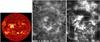 |
Fig. 1 Active region AR 11850 observed on September 24, 2013 from left to right: full disk image in AIA 304 Å, the white box indicates the field of view of the two right panels (140 × 175 arcsec2), Hα image (MSDP/Meudon spectrograph) and Mg II k line centre at 2803.5 Å obtained between 11:43 and 12:04 UT (IRIS spectrograph) showing the arch filament system (AFS). The two white boxes in the IRIS panel represent the field of view of the two small rasters presented in Figs. 3 and 4. |
EBs have also been observed in EUV continua at 1600 Å and 1700 Å, which are mainly formed in the low atmosphere, with TRACE and the Solar Dynamic Observatory (SDO/AIA) and show rapid variations of intensity (200 s) (Pariat et al. 2007; Vissers et al. 2013). The signature of EBs in the upper atmosphere is not clear. Pariat et al. (2007), Vissers et al. (2013) discussed on the observation of a EB related to a brightening observed in UV. This brigthening could correspond to the plasma of a surge-like event emitting in the C IV line at 1548 Å, which is also present in the 1600 Å passband. The association of Hα EBs and bright points at coronal temperatures in 171 Å (TRACE, AIA) and in X-ray (Yohkoh/SXT, Hinode/XRT) is rare. In the data of FGE, only one bright feature was detected in 171 Å (TRACE) and in X-ray and associated with one EB among the 47 identified EBs (Schmieder et al. 2004), and again it is possibly a jet.
The Interface Region Imaging Spectrograph (IRIS) with its high spatial resolution (pixel 0.167 arcsec, resolution of 0.3 arcsec), launched in June 2013 (De Pontieu et al. 2014) revealed the existence of bright points in the Mg II h and k chromospheric lines, and also in Si IV, CII and the Mg II triplet lines, which are formed in a wide range of temperatures (Peter et al. 2014; Vissers et al. 2015). These bright features are very intriguing because they are not visible in O IV lines and the Si IV profiles are blended by photospheric lines that are visible in absorption. Peter et al. (2014) called them “hot explosions in the cool atmosphere”. Vissers et al. (2015) investigated the IRIS signatures of Hα EBs. Among the large number of detected Hα EBs in emerging regions, only a few of them were in the field of view of IRIS spectra and/or have an IRIS brightening counterpart signature.
Archontis & Hood (2009) aimed at reproducing EBs via low atmospheric reconnection. The recent model of Archontis & Hansteen (2014) is very promising for mimicking the hot bombs. However the current sheet where the reconnection can occur is located in the corona. This model as it is cannot really explain the lower atmospheric formation of the bombs described by Peter et al. (2014).
Thermodynamical models of EB spectra are based on NLTE radiative-transfer modelling in a simple 1D plane parallel semi-infinite atmosphere (Kitai 1983; Fang et al. 2006; Socas-Navarro et al. 2006; Herlender & Berlicki 2011). Semi-empirical models assume the hydrostatic equilibrium. However owing to readjustment of the kinetic temperature, heating is found not only in the photosphere, but also in the upper chromosphere. Recently Berlicki & Heinzel (2014) constructed a grid of models based on a model of a quiet solar atmosphere and introduced a hotspot region at the photospheric level. By adjusting the four variable parameters for the hotspot (width, peak of temperature, density, position), they were able to fit the contrast of EBs observed in Ca II and Hα wings by the Dutch Open Telescope (DOT) instrument in LaPalma.
We had the opportunity to observe the emerging flux occurring in the AR NOAA11850 located at N08, E10 (x = −310 arcsec, y = 100 arcsec) on September 24, 2013 during the 60-day first joint observations of IRIS with the Télescope Héliographique pour l’Étude du Magnétisme et des Instabilités Solaires (THEMIS) magnetograph in Tenerife (Sect. 2), and the Multi-channel Subtractive Double Pass (MSDP) spectrograph (Mein & Mein 1988) operating in the Meudon solar tower. Extended arcades of filaments called an Arch filament systems (AFS) overlying the region, direct signatures of an emerging flux, are well visible in MSDP Hα and IRIS images (Fig. 1).
We focus our study on the Mg II, Si IV, and CII spectra observed with IRIS and Hα observed with THEMIS. The Hα observations are not co-temporal with IRIS observations and cannot be used to detect EBs directly as in the paper of Vissers et al. (2015). However we used the properties of the chromospheric EB spectra for the selection of the compact bright points (CB), which could possibly be recognized as an EB. EBs are perfectly detectable in the wings of chromospheric lines and are distinct from bright network points owing to their emission in a much wider wavelength domain, including far wings. Our selection of CBs is restricted to the field of view of flux emergence and is based on the brightening enhancements in the Mg II line wings by analogy to this chromospheric line behaviour in the visible range (Sects. 3 and 4). Tian et al. (2016) confirmed that the Mg II k and h lines can be used to investigate EBs that are similar to Hα. With the 1D model of Berlicki & Heinzel (2014) developed for Hα, we compute the corresponding grid of profiles for Mg II lines (Sect. 5). We note that this model does not take into account the dynamics of the plasma and will therefore not explain the physics of the formation of the CBs. We compare the observed profiles with the synthetic profiles to determine the position and the extension of the hotspot in the temperature profile of the atmosphere, which could correspond to the heating that is due to magnetic reconnection (Sects. 6 and 7). We conclude on a large dispersion in these altitudes from the deep photosphere to the chromosphere (Sect. 8). We discuss the effects of introducing a cloud model by using a 2D NLTE modelling of fibrils. Our codes are limited to chromospheric temperatures and we have no information about higher reconnection altitudes in the atmosphere or heating to higher temperatures. The models proposed to fit the observed Mg II profiles produce Hα profiles that are consistent with the observations of THEMIS and the SST (Vissers et al. 2015).
2. Observations
2.1. THEMIS
The THEMIS instrument (López Ariste et al. 2000) was used in the Multi Temperature Raies (MTR) mode with two cameras. One camera recorded the four Stokes parameters in the 6302 Fe I line to do spectro-polarimetry and in the Hα line, i.e. see I+V and I-V image in Fig. 2 (top panel). We use the Hα spectra rastering the active region between 08:02 UT to 09:25 UT and 09:35 UT to 10:35 UT, which is just one hour before the IRIS observations. After removing the trend caused by instrumental effects, we calibrate the Hα spectra by using the David reference observed profiles (David 1961) following the method described in Berlicki et al. (2005). Firstly we determine a mean profile by averaging profiles along the slit containing an EB, but avoiding the EB profile. This mean profile is considered as our reference quiet Sun profile. We fit it with the David profile to obtain an absolute calibration, after taking into account the position of the slit in the Sun disk and the limb-darkening effect. The EB profile is calibrated in a second step with the same procedure. Figure 2 (bottom panel) presents the quiet Sun David profile, our reference quiet Sun profile, which fits well the David profile owing to its definition, the profile of one THEMIS EB, and the synthetic Hα profiles that we computed using the five NLTE models, each one determined by fitting an observed Mg II profile of a selected CBs (Sect. 9).
IRIS lines of interest (rest wavelengths from the line list of Sandlin et al. 1986).
2.2. IRIS
IRIS performed two large dense rasters for 20 min, each covering the whole active region from 11:43 UT to 12:04 UT and from 15:39 to 15:59 on September 24, 2013 (OBSID ref. 4000254145). The centre pointing of the rasters was (x = −265.46 arcsec, y = 87.96 arcsec) for the first raster, (x = −264.55 arcsec, y = 70.35 arcsec) for the second raster. The spatial pixel size is 0.167 arcsec. Both rasters (140 × 175 arcsec2) consist of 400 spectra with a step size of 0.35 arcsec and taken with a cadence of less than 3 s. The rasters are obtained in a large number of lines in the near ultraviolet NUV window: 2783 to 2834 Å and the two far ultraviolet windows: FUV1 1332−1348 Å and FUV2 1390−1406 Å wavelength bands. Table 1 gives the list of lines of interest for this study. During the 20 minutes of the raster acquisition, slit-jaw images (SJI) (175 × 175 arcsec2) were registered in the broadband filters (2796 Å and 1400 Å) with a cadence of 12 s and in 2832 Å with a cadence of about 80 s. The 1400 slit jaw intensity is an integration of the FUV emission within a range of about 55 Å, including the total emission of two Si IV 1402/1393 Å lines, the 2796 SJI intensity is integrated over 4 Å around Mg II k 2796.35 Å line. The Mg II h, and k are formed at chromosphere plasma temperatures (104 K). The ionization of the Mg II element occurs for a temperature equal to 2 × 10⁴ K. The SJI 2796 Å filter gives images of the chromospheric temperature plasma. The 1400 Å filter is a combination of the UV continuum formed at the temperature minimum and the emission of the Si IV lines formed at the transition region temperature. The co-alignment between the different channels is achieved by checking the position of the horizontal fiducial lines present in the spectra. Our main goal is to model the Mg II lines and compare them with the IRIS observations. We present the Si IV and CII spectra of the detected Mg II bright points for discussion.
2.3. IRIS data radiometric calibration
We downloaded level 2 data from the IRIS data base for our study (De Pontieu et al. 2014). IRIS spectra are given in the units of counts (DN). We calibrate the IRIS data based on the area response of the spectrograph from the preflight calibration (IRIS technical Note 24). We convert DN, after dividing it by the exposure time to observed intensity (Iobs [DN / s]) into physical units (Iabs [erg s-1 cm-2 Å-1 sr-1 ]) in the following way: 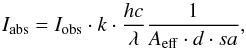 (1)where k is the number of photons per DN (4 in the case of NUV and 18 for FUV spectra). In our calculations, we have the following values: Planck constant h = 6.63 × 10⁻²⁷ erg, speed of light c = 3 × 1010 cm s-1, λ [cm]. The effective area Aeff is available in SolarSoft through iris_get_ response(), d = 0.0254 Å × pixel-1 is the dispersion. We need also the solid angle sa, which is
 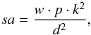 (2)where w is the slit width (0.33 arcsec), p pixel size along slit (0.167 arcsec), k (km per arcsec (727.1 km), and d distance to the Sun (1.5 × 10⁸ km). After calculation sa is equal to 1.2949 × 10⁻¹² arcsec2. To calibrate the data at Si IV 1394/1403 Å and C II 1336 Å, we used a similar procedure, but with different values of the effective area and dispersion. For Si IV d = 0.01298 Å × pixel-1, for C II d = 0.01272 Å × pixel-1.
3. Compact brightenings in Mg II lines
3.1. Mg II spectroheliograms
From the two recorded rasters of IRIS spectra, we create spectroheliograms of the active region in Mg II h line at specific wavelengths: Δλ = −3.5 Å, Δλ = 0 Å, Δλ = + 0.23 Å, Δλ = + 1 Å (Figs. 3 and 4) to visually detect CBs, which we examine in the context of searching EBs. Therefore we reduce the size of the studied areas to two smaller regions concerned only with the flux emergence, which were recorded in 11.5 min from 11:49−12:00 UT (raster 1) and from 15:46−15:58 UT (raster 2) (white boxes in Fig. 1 right panel), regions where the AFS are well visible in Hα and Mg II h3 line centre images (Fig. 1). Each CB emission covers 1 to 6 pixels along the slit as is shown in the top panels in Fig. 5. Figure 6 (bottom left panel) gives an example of three different profiles in the CB (B). The adjacent spectra at +/−0.35 arcsec did not show a clear enhancement of emission. This indicates that the size of the CB is around one arcsec. Comparing the spectroheliograms of these two smaller regions shown in Figs. 3 and 4, we note the difference of appearance of CBs according to their wavelength. At λ = 0.23 Å, which represents the common position of the Mg II h peaks (h2v, h2r), AFS and some bright CBs are observed. More CBs are detected in the wings of the Mg II lines, i.e. at Δλ = −3.5 Å (top panel) and Δλ = + 1 Å (middle panel). The brightenings of some CBs are, nevertheless, very weak in the far wings and not detectable in SJI 2796 Å because of the low intensity in their peaks, h2r and h2v. The contribution of the emission of the peaks of the near-by chromosphere can be more important than the increase of emission in the wings in these CBs and diminish the contrast of the CBs in the SJIs, which are recorded in a relatively small wavelength band pass (4 Å) centred on the peaks compared to the broad Mg II k line extension over 13 Å. These CBs detected in the far wings do not always have a corresponding CB detectable in h2v-h2r as we will discuss in the examples in Sect. 4.2. We decided to analyze mostly the Mg II h line (and not Mg II k) in the spectra because of the IRIS spectral window range is limited in the blue wing of Mg II k line at −2 Å from the k line centre, while the red wing of h line is observed up to 4.5 Å. Then the modelling of the Mg II h line can be completed in its far red wing. This is better for the comparison between synthetic and observed profiles (Sects. 5 and 6). In Fig. 3, we add the spectroheliogram obtained in the continuum at +26.6 Å of the Mg II h line centre. Some bright points in the continuum are still visible.
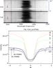 |
Fig. 2 Top panel: spectrum of an EB in H α line observed by THEMIS/MTR spectropolarimeter. The two red arrows indicate the EB in I+V and I-V channels. Bottom panel: Hα profiles – Observed profiles: EB profile of the THEMIS spectrum shown in the top panel (solid black line), observed nearby quiet Sun profile from THEMIS (thin black line). Synthetic profiles computed from NLTE modelling: QS (purple solid line). All colour profiles described with letters from A to E are calculated for each best model of selected CBs (A − red; B − orange; C − light green; D − light blue; E − dark blue). Intensity units is (erg s-1 cm -2 Å-1sr-1), Δλ unit is Å. |
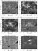 |
Fig. 3 AR 11850 IRIS observations of raster 1 (the field of view is indicated in Fig. 1, right panel). Top and middle panels from left to right: Mg II spectroheliograms at 2800.0 Å, 2803.5 Å, 2803.7 Å and 2804.5 Å. Bottom left panel: spectroheliogram in the continuum at 2831.1 Å. Bottom right panel: spectroheliogram in Si V line. White or dark boxes show the selected CBs from A to D (the numbers in parenthesis indicate the hot explosions of Peter et al. 2014), small white circles with numbers 5 to 9 in the second row, right panel are examples of small brightenings. |
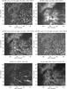 |
Fig. 4 AR 11850 IRIS observations of raster 2 (the field of view is indicated in Fig. 1, right panel). Top and middle panels from left to right: Mg II spectroheliograms at 2800.0 Å, 2803.5 Å, 2803.7 Å, and 2804.5 Å. Bottom left panel: spectroheliogram in Si IV line. Black circles in Mg II +0.1 Å and in Si IV spectroheliogram indicate CBs visible in Si IV and Mg II line wing. Bottom right panel: slit-jaw image at 2796 Å. The white box indicates the location of the CB (E) that we have analysed. The EB (E) is not visible in Si IV and Mg II core of the line. |
Since our radiative models used as the basis for the spectral synthesis cannot emulate dynamics, we select the less asymmetric profile in each CB. Figure 6 (left bottom panel) gives an example of our selection for the CB (B) which presents emission in six pixels along the slit for one spectra. B2, B3 pixels have asymmetric profiles in Mg II h line and in Si IV lines. We choose B1 for the CB (B). This profile corresponds generally to a pixel in the central part of the CB.
3.2. Statistics of the bright points
We count the compact bright points in the restricted emerging area where AFS are visible. For raster 1, 42 CBs are identified in the image in Mg II h line at Δλ = −3.5 Å with a contrast better than 2, while only 38 of these 42 CBs are still visible in the image at Δλ = + 1 Å. For raster 2, the numbers are similar (36 CBs) if we take into account that a part of the emerging region is cut. The global number of CBs in the two rasters is 74.
Let us see how many are detected in hot temperature lines. In the slit jaw images at 1400 Å corresponding to the field of view of raster 1, only four brightenings are identified (see Fig. 1 in Peter et al. (2014). For the field of view of raster 2, the number of brightenings in spectroheliogram at 1402.8 Å and in SJI 2796 is difficult to be evaluated owing to the bright elongated structures but can be estimated as 4 to 5. They correspond to the CBs observed in the wing of Mg II at 1 Å (Fig. 4 bottom left panel and middle right panel). The emerging flux is between x = −160 and x = −135 and y = 38 to 80 arcsec. Four brightenings are detectable but mixed with bright fibrils overlying the region. Finally among the 74 CBs detected in Mg II lines, only eight brightenings have a signature in hot lines (Si IV and CII). We conclude that the number of bright points in SJI images is about ten times smaller than the detected Mg II CBs.
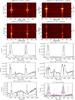 |
Fig. 5 Spectra and profiles of Mg II h and k and Mg II triplet at 2798.7 Å lines for the five selected CBs. Two top rows: spectra of the CBs shown in the boxes of Figs. 3 and 4. The arrows indicate the positions of each CB: A to E at y = 47.5, 59.0, 50.9, 52.7, 74.2 arcsec, respectively, where the profiles are taken and drawn below. Bottom five plots: profiles of A to E (solid line) with the QS (dotted line) and the nearby quiet profile (dashed thin line). Bottom right panel: plot of all the selected profiles shown in a different colour: A − purple; B − green; C − blue; D − red; and E − black. Intensity units is (erg s-1 cm -2Å-1sr-1), wavelengths unit is Å. For CBs C and D, we note that the emission of Mg II triplet is enhanced and its line profile is absorbed by an Mg II line (2798.6 Å) in the blue wing and by an Mn I line (2799.2 Å) in the red wing. |
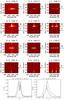 |
Fig. 6 Four top rows: spectra of Si IV 1394 Å , Si IV 1403 Å, and C II 1336 Å of the five selected A to E CBs. Bottom left and right panels: example of multi structures in CBs along the slit: Mg II h and Si IV 1394 Å respectively profiles in the CB B: B1 identical to B for y = 59 arcsec (pixel = 374) (solid line), B2 for y = 59−0.33 arcsec (pixel = 372) (dashed line), B3 for y = 59 + 0.5 arcsec (pixel = 377) (dashed-dotted-dotted line), with profiles outside the bomb (y = 61.5 arcsec (pixel = 389) − dashed-dotted line). The bright spectra with a large blue shift below B is not considered as belonging to CB B. The Si IV 1393.76 line blue wing is ragged by two absorption lines (Fe II at 1392.2 Å) and Ni II (1393.3 Å) for CBs A B, and D. Intensity units are in (erg s-1 cm -2Å-1sr-1), wavelengths unit is Å. |
After looking at the Fig. 1 of Vissers et al. (2015), comparing Hα EBs and bright features visible in Si IV and CII lines, we can estimate a similar result. This should be checked certainly in more details.
Finally, we focus our study on five selected CBs which are representative of the full sample. All the CBs that we have studied are observed in the far wings of Mg II lines because of our selection criteria. Only a few of them (10%) have large intensity peaks or very wide profiles. The selected CBs are shown in Figs. 3 and 4 (white boxes indicated by the letters A to E). The CBs (A) and (B) are the best visible in the Mg II spectroheliograms at Δλ = + 0.23 Å (peaks) and Δλ = + 1.0 Å (Fig. 3). We can hardly see that the CBs (A) and (B) in the far wings (Δλ = −3.5 Å). The CB (C) is not visible in the panels at Mg II line centre (the bright line could be due to a bright fibril) and in the peaks. The CB (D) are visible in each panel in Fig. 3, except in the panel at Mg II h line centre where a dark fibril is instead observed. The CB (E) is visible in the spectroheliograms obtained in the far wing of Mg II line at Δλ = + 1 Å and Δλ = −3.5 Å (Fig. 4).
Three of the selected CBs have a signature in the Si IV spectroheliogram (Figs. 3 bottom right panel). The CBs named A, B, and D correspond to the hot explosions 3, 4, and 1, respectively cited in Peter et al. (2014). The other two CBs, C and E, have no signatures in Si IV spectroheliograms. Our main goal is to find and determine which CBs visible in Mg II lines could correspond to EBs by also modelling the Hα line with the same atmosphere models. We perform a radiometric calibration of the Mg II spectra, which has not been achieved earlier for this data set in order to compare the observed profiles with synthetic profiles computed from NLTE models.
4. IRIS spectra and profiles of the CBs
For the five selected CBs, we present the concerned Mg II spectra along the slit and point by an arrow the pixel inside the CB (A to E) (Fig. 5 top panels). The corresponding profiles are presented in each panel in Fig. 5 bottom panels, and all are summarized in the bottom right panel to see their differences in one glance. The Mg II h and k lines and the two lines of the Mg II triplet between them are observed in a unique spectral window of IRIS around 13 Å wide. In the same way, we present the SiV and CII line spectra along the slit and profiles of the five pixels, one or two CBs are in each spectra (Fig. 6).
4.1. Quiet Sun profiles
The quiet Sun profile (QS) (average profile from IRIS observations of disk centre at 04:20 UT) and a local quiet Sun profile (QSloc), obtained by averaging 20 profiles of Mg II h spectra observed out of the CB along the same slit position, are also presented in Fig. 5. The QS profile is very similar to the Mg II profile determined by Staath & Lemaire (1995). The QS profile of Mg II lines consists of a large absorption profile of more than 20 Å wide with two pairs of emission peaks, one for h and one for k Mg II lines, in the central part of the absorption profile. The IRIS window (13 Å) is centred in this absorption profile in the middle of the Mg II h and k lines. In the following work we concentrate on the Mg II h line which, in our observations, presents a more extended red wing than the blue wing of k. The two peaks of the h line have a maximum of intensity of 4 × 10⁵ erg s-1 cm-2 Å-1sr-1, a FWHM of 0.2 Å, the centre of the line an intensity value of 1.5 × 10⁵ erg s-1 cm-2Å-1 sr-1, and the separation of the two peaks a distance of 0.4 Å. The mean profiles of the Mg II lines close by the CBs (QSloc) have the same absorption profile in the IRIS window, but slightly higher intensity in the peaks and in the line centre than the QS. The FWHM of the peaks and their separation are unchanged.
4.2. Characteristics of the CB line profiles
The global shape of Mg II k and k lines is similar in CBs, as can be checked in Fig. 5. We focus our analysis on the Mg II h line profile because of its extending red wing, as we explained above. The line profiles of (A) and (B) have a strong Mg II peak intensity (h2v and h2r). Their intensity is by one order of magnitude higher than the peaks of the QS profile and by a factor 2 with the peaks of QSloc (Fig. 5, middle panels). Their FWHM is of the order of 1.5 Å. The centre intensity h3 in the Mg II h line for (A) is comparable to h3 intensity of QSloc profile. Its value is around 1 × 10⁵ erg s-1cm-2 Å-1 sr-1. On the contrary h3 for B is increased to 2.1 × 10⁵ erg s-1cm-2Å-1sr-1. We note that (A) and (B) have a strong emission in Si IV, CII lines (Fig. 6).
For (C), the Mg II h spectrum presents an emission enhancement in the two peaks particularly in h2v, but the values of the emission do not reach the h2 values of (A) and (B) spectra. Additionally a strong emission enhancement is noted in the far wings (Fig. 5). The emission is over the whole wavelength range. The h3 emission reaches nearly 1.5 × 10⁵ erg s-1cm-2Å-1 sr-1, which is more than the QS loc. The Mg II h profile of (C) presents a strong peak asymmetry, which indicates the presence of either material flows or overlying dynamical fibrils. The CB (C) has no counterpart in Si IV and CII spectra (Fig. 6). However the Mg II triplet intensity in (C) is enhanced and shows the same asymmetry as the Mg II h and k lines.
 |
Fig. 7 Intensity profiles of Mg II lines for events that have high intensity in the wings and small intensity in the peaks. The selection was done randomly (see the small circles in Fig. 3). The correspondence is as follows: 5 − dark blue; 6 − light blue; 7 − red; 8 − orange; 9 − light green. The black line represents the E profile. All these profiles have a shape between CB C and CB E profiles. |
Parameters of the observed Mg II line profiles.
The (D) brightening, according to Table 2 is, in many respects, similar to the C brightening, however it reveals certain differences owing to the raggedness? of the D profile, for example (Fig. 5). The two peaks h2v and h2r are very broad, separated, ragged and irregular, as was mentioned in Peter et al. (2014). The intensity of the peaks is comparable to the h2 intensity of the QS loc profiles (dashed lines in Fig. 5), but the line centre intensity h3 is lower than h3 of the QS loc, which is nearly equivalent to the h3 value of the QS. The wing emissions are several times higher than in the case of both the quiet Sun wing emissions (QS and QSloc). This CB (D) has a strong emission in the Mg II triplet between the h and k Mg II lines around 2798.5 to 2799.5 Å and strong emission in Si IV and CII lines with absorption of photospheric lines, which suggests the presence of a cloud of cool material along the line of sight at the location of the CB (D).
The (E) spectrum presents a completely different type of event. Bright emission is visible with small intensity differences between the peaks and the far wing emission. The Mg II h profile has peak intensity values (h2v and h2r) that are only double the QS peak intensity. and more than 50% even lower than the QSloc. Peak emission is around one order lower than for the other CBs. CB (E) spectra in Si IV, CII lines, and Mg II triplet present no emission (Fig. 6). Type (C) to type (E) profiles are the more frequently observed CB profiles, see some other randomly chosen profiles (Fig. 7). They correspond to small CBs, shown by small circles in the spectroheliogram obtained in Mg II h–1 Å (Fig. 3, second row right panel).
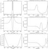 |
Fig. 8 Examples of synthetic profiles for different models: chromospheric 53-5, model of the hotspot in low chromosphere, close to the temperature minimum region 65-7 and photospheric model 77-6. For each model a different part of the profiles is enhanced. |
4.3. Classification of the Mg II compact brightenings
After the detailed analysis of the Mg II profiles of the five CBs, we determined three different types of brightenings. We believe that later on, this will allow us to find some EBs among them. For each selected CB, we determine the following parameters of the Mg II h profile: peak separation, line centre intensity, peak mean intensity, integrated intensity (with range: −/+ 1.7 Å). These values will be useful in the next part on our analysis, for comparison with the synthetic profiles. All of these profile parameters are shown in Table 2. Three types have the following characteristics: (1) enhancement emission in peaks and close wings; (2) enhancement emission in peaks, close wings, and far wings; and (3) enhancement emission only in wings, close and far, and untouched in the peaks and line centre. We also note that the lower the emission is in the line, the higher the emission is in the wings and far wings. Our division is as follows: CB (A) and CB (B) brightenings represent the first type, CBs (C) and (D), the second type, the third type is the CB (E), which are very common features in our field of views in Mg II lines (Figs. 3 and 4). To characterize properties of profiles and test our classification a posterioriin three groups, we calculated the contrast values in comparison with the quiet Sun profile for each brightening for three wavelengths (h3, h2 and δ(λ) + 3.5 Å). The contrast is defined as follows:  (3)where ICB is the intensity of the compact brightening and IQS is the intensity of the quiet Sun. These values of contrast are presented in Table 2.
Type 1 CBs have a strong contrast in the line centre and also in the mean peak, type 2 CBs have a high contrast in the far wings, type 3 also has a high contrast in the far wings, but no contrast in the mean peak.
The five CBs that we selected have different Mg II profiles with different characteristics and different counterparts in Si IV, CII, and the Mg II triplet. This different behaviour helps us to clarify our selection of CBs in type 2. The Mg II triplet is particularly visible in the type 2 spectra of our selection CB (C) and (D) with enhancement of the emission to 1−1.2 × 10⁶ erg s-1 cm-2 Å-1 sr-1. This is why they belong to the same type. However, they present a strong difference in their signatures in the Si IV and CII lines. Therefore we classify CB (C) as type 2a and CB (D) as type 2b. Types 1 and 2 b commonly have strong signatures in hot temperature formation lines.
In Table 2, we add a line on the emission in Si IV line of each CB (Y/N) and the h2v/h2r ratio in Mg II h line, indicating the degree of asymmetry of the profile. The value of the h2v/h2r ratio is close to 1, indicating that the selected profiles are more or less symmetrical. Each category represents typical profiles that are observed.
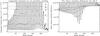 |
Fig. 9 Left panel: example of one profile parameter, such as the right integrated intensity obtained for all models. The horizontal lines on the diagram represent the values of the parameter for the observed profiles − dotted line for A brightening, dashed line for B, dashed dotted line C, dashed-dotted-dotted-dotted for D and long dashed line for E. Right panel: the square root of the mean-square intensity difference between synthetic and observed profiles: one example of the A brightening. The best model for A is N = 120. |
The paper of Vissers et al. (2015) presents different IRIS profiles of CBs which overlay spatially and co-temporally Hα EBs observed with the SST. Some of our CBs present similar morphological characteristics and belong to this special category of CBs selected with a different criteria. The three CBs (A, B, and D) follow their criteria, being visible in Si IV. In fact they have either large emission in Si IV lines or wide profiles. Our CB (A) which is the bomb 3 of Peter et al. (2014) and our CB (B) have similar profile as EB2 in Vissers et al. (2015). They could be considered as Hα EBs and hot explosions. In relation to the distinction between the flaring active filament (FAF) and EB, the profile D (hot explosion 1 in Peter et al. 2014) is, maybe, an FAF as mentioned by Vissers et al. (2015) and not an EB in an early stage of life, but in a later phase when the AFS are making a strong canopy over the region.
The two other CBs of our selection, C (type 2a) and E (type 3), which are the more frequent in our selection (see Fig. 7) did not fit the Si IV criteria but we will see that the NLTE model that fits the Mg II profile of CB(E) reproduces well the Hα EB that we have observed with THEMIS.
In summary we propose the following statistics concerning the 74 CBs that we have detected in raster 1 and raster 2 in the emergence areas: 10% are similar to type 1, only one CB has an Mg II profile like CB (D) (type 2b), 10% to type 3 and 80% are between type 2a to type 3. For this analysis, we looked at each CB Mg II line and Si IV line profiles.
5. NLTE modelling of Ellerman bombs
5.1. Mg II line modelling
To calculate the synthetic line profiles, we use a multilevel NLTE radiative-transfer modelling. The multilevel NLTE transfer problem is solved by using the multilevel accelerated lambda iteration technique (MALI) of Rybicki & Hummer (1991, 1992) and the linearization scheme to take into account the hydrogen ionization equilibrium (Heinzel 1995). This solves the radiative transfer and statistical equilibrium equations for our model of Mg II ion. In this study, we use a five-level plus continuum Mg II-Mg III model atom. Apart from the two strong h and k resonance lines, we also include three line transitions between the 3P and 3D states (Mg II triplet see Table 1). These subordinate lines appear just close to the h and k lines (2790.8, 2797.9, and 2798.0 Å). However, they are generally very weak and relatively far from h and k line peaks. Based on Milkey & Mihalas (1974) (with the reference to Dumont 1967), who showed that these and other subordinate lines have a negligible effect on the source function of the resonance lines, we thus neglect other line transitions to 4S state and to higher states. For our 1D modelling of EBs, this model of Mg II is fully sufficient. Finally, we solved the NLTE transfer problem and we synthesized the emergent hydrogen line profiles of EB. In the next step, we used the same model and computed electron densities to synthesize the Mg II h and k spectrum. Mg II h and k lines are treated with PRD, which is very important in the line wings. Atomic data and collisional rates provided by Shine & Linsky (1974) and H. Uitenbroek (priv. comm.).
5.2. Grid of models
We used EB models based on a simple 1D plane-parallel, semi-infinite atmosphere. The construction of atmospheric model of EBs was discussed in Berlicki & Heinzel (2014). These models were constructed by placing a local temperature increase (LTI, also known as a hot-spot) structure at a given altitude in the solar atmospheric model of the quiet Sun. The modelling performed in this study does not take into account the dynamics and will therefore not explain the asymmetry of some Mg II profiles. We used the semi-empirical model C7 developed by Avrett & Loeser (2008). To find the best models that fit our observed profiles, we created a grid of models where the temperature structure is modified within the hotspot. Our model parameters are: the position/altitude of the hot spot and its width and peak temperature increase. Similar to Berlicki & Heinzel (2014), our grid of models consisted of 243 models. We chose 27 different positions of the hotspot, every 40 km, from 50 km above Sun surface (τ500 = 1) to 1500 km. For each position in the solar atmosphere, we have nine different models with different values of the temperature increase. The width of LTI does not change. Mass density of the hot spot is taken from a C7 model and we did not modify it. The sensitivity of the results to the density has been tested in Berlicki & Heinzel (2014) and they concluded that the sensitivity was weak and the best fitting was obtained without changing density in CBs. In Fig. 8, we present some representative examples of the temperature profiles of some models from our grid. The names of models consist of two numbers − the first number from 52 to 78 (respectively 1500 and 50 km) represents the position in the atmosphere and the second number represents the temperature increase of the hot spot, from 1 (for 1100 K) to 9 (for 5500 K). For each model, we computed the synthetic spectra of the Mg h and k lines.
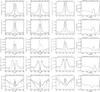 |
Fig. 10 Plots with the results of modelling. The first two left columns show some synthetic profiles (solid line) compared with observational profiles (dashed line) for best models from the grid. Some of the profiles are chosen from method based on profiles parameters, some of them have additional profile chosen after visual verification (63-5 for B, 73-1 for C, 68-4 for D, 75-1 for E). The third column presents the synthetic profiles (solid line) obtained from modified models compared with observational profiles (dashed line). In the last, right column, we present the temperature structure of the best models plotted with a black solid line. The dashed line represents models before modification. In this figure, each row corresponds to other compact brightening from A to E, respectively. |
It is well known that Mg II h and k lines are formed in the wide range of the chromosphere and upper photosphere and different parts of the line profiles come from different heights (Leenaarts et al. 2013a,b; Pereira et al. 2013). Therefore, magnesium h and k lines are good indicators of the atmospheric conditions. The greatest opacity is in the line centre and this part of the line is formed in the upper chromosphere. Further parts of the line profiles are formed deeper in the atmosphere. This relation is also clear in our examples (Fig. 8). For LTI placed high in the atmosphere, we obtain strong narrow peaks and a small emission in the wings. The deeper we move, the more the emission is enhanced and moves further away from the line centre and the peaks get wider, because of combined emission in peaks and close wings. For hotspots located around the temperature minimum, the emission in far wings became much stronger but the line peaks are still enhanced. For hotspots located even deeper in the photosphere, the emission is strongly enhanced only in the far wings, but the line centre intensity decreases and become close to the quiet Sun intensity of both Mg II lines.
6. Comparison of the observed and synthetic spectra
The grid of models contains a great number of hotspot models (N = 243). Our goal is to find the best model of each selected bright Mg II bright points from these N models. To compare synthetic and observed line profiles, we take into account four different parameters of each profile, both for the synthetic and the observed: peak separation, intensity of the peak (in the case of observed spectra we took average intensity from two peaks), intensity of the line centre and integrated intensity (Table 2). Integrated intensity was computed in the range from −1.7 Å to + 1.7 Å. In Fig. 9 (left panel), we show for each model the value of the integrated intensity parameter as an example. Five different horizontal lines in the plots represent the values obtained from observations. If the line passes through the value of this parameter for some models (diamond points), it means that this value fits with the observation. At first glance, many of the models fit the observations reasonably well. The method of looking for the best model through parameter fitting is not fully effective. The problem is that the model that is the best according to one parameter, is not good for another one. Our code does not include plasma flows, which may be important in the Mg II line formation. In the observed CBs, many Mg II line profiles have asymmetric peaks, however, our selection was restricted to symmetric profiles where the asymmetry of peaks are not significant, suggesting that the velocity of the emitting plasma is low. This weak flow should not affect all four parameters, which were used for model determination, but mainly the separation and the intensity of the peaks. Peak separation or line centre intensity do not seem to be a proper parameter to determine the best model. From the whole set of best models, we can derive some kind of distribution of models for each parameter, which can tell us about the approximate region of the atmosphere, where the CFs are forming: are they in the photosphere or rather in chromosphere? If we knew that, we could narrow down our search for the best models.
Our analysis showed that the most suitable parameter for the model determination is the line-integrated intensity. For each given line, emitted under specific conditions, the shape of the profile can be different because of the Dopplershifts, but the total emission, represented by integrated intensity, should be the same. We also computed the mean intensity difference between all synthetic profiles and each observed profile (in the wavelength range: 2800.8−2806.5 Å) in the following way: 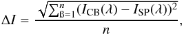 (4)where ICB is the intensity of the compact brightening, ISP is the intensity of synthetic profile, n is the number of wavelength points across the line profile. Figure 9 (right panel) presents one example diagram of the mean-square intensity difference between all synthetic profiles and the observed profile for compact brightening A. The best models have the lowest values of mean-square intensity difference, e.g. for A it is N = 120.
7. Models of bright points obtained from Mg II line profiles
All the presented methods of fitting the theoretical and observed line profiles only give us an approximate model. General properties of hotspots (position, temperature, and width) are presented in Table 3. If we consider each fitting parameter separately, we get some indication of the hot spot parameters: the approximate position in the atmosphere and the temperature increase. Each N model is defined by two numbers, one characterizing the position and one the temperature. The model for which there is a convergence towards these two parameters was chosen as the best model, after a visual inspection. Some models of CB were not found by our methods and we had to apply a new type of model with two hotspots.
In Fig. 10, we present the results of the modelling using the method described in the previous section. In some cases a modification of the models is required, because of the adopted discretization of temperature and the unique value of the width for each peak. It can happen that the modelled temperature of the hotspot or the width of the line peak has to be between two grid values to obtain the best agreement with observations. We noticed in Fig. 10 that for A brightening the fitting is not perfect, the peaks are too small, but we can change it by raising the temperature of the peak slightly in the two chosen models (64-5, 65-5). The profile calculated with the model 64-5 has too small an emission in the wings, and too narrow peaks. In the case of 65-5 model, we have the opposite situation, despite this model being different only by its position in the atmosphere, by around 40 km. The hotspot of this model is at a height of around 630 km above the Sun’s surface, in the low chromosphere. We can assume that if we also modify the width of the temperature peak, we can link these two models as one.
In the case of fitting the B brightening, we have a similar situation, the best model is also (64-5), but it required higher temperature peaks. Additionally, we chose model 63-5; it has smaller emission in the wings and higher and narrower peaks. By expanding and increasing the temperature of LTI we obtain broader peaks (Fig. 10). The problem with the line centre and intensity in wings is similar to the A brightening case. In this profile, we have a red asymmetry of the peaks, which indicates the presence of flows. B brightening represents a dynamic event and the profile presents a red asymmetry, as can be seen in the spectrum (for cut y = 374, for other cuts profiles is changing diametrically). For now, we do not focus on the dynamics of the events, but this should be taking into account in future analysis of this phenomena, especially sunce it can be a signature of explosions, which have strong influence on the profile and on the model of the phenomena itself.
Also D brightening has quite a good fitting and the best models for this event have peaks placed deeper in the atmosphere and have a lower temperature LTI. Model 68-4 is chosen by our methods and model 67-4 is an additional model, chosen by visualization. The profile obtained from model 68-4 for D brightening does not correctly fit the wing and peak intensity, even after modifications (Fig. 10). Therefore, we selected the other model, 67-4, in which we change the width of the LTI and the increase the temperature. The fitting is better for the red peak. Nevertheless the observed profiles cannot be completely recovered because the observed line centre is blueshifted (owing to flows), and the peaks are asymmetrical and jagged, which again indicates the presence of dynamic properties of plasma.
We had a bigger problem with C and E brightening. Examples of C and E events reveal that the temperature structure of LTI is more complex. Increased intensity, both in the peaks and in the wings, indicate a very broad region of the atmosphere where the temperature was increased. Even a small enhancement in the peaks of E profile, needs some LTI higher in the atmosphere. The very first step in finding the best model is a simple combination of these two best models.
C and E brightenings require a different treatment if we want to obtain a better fitting. In both, C and E cases, we take two models for which some parts of the synthetic profiles were in agreement with the observational profiles and we combined the profiles together. Then we modify these linked models, to obtain the best possible fitting, by rising or decreasing the temperature in this region of the atmosphere, where particular parts of the profiles are formed. For C brightening, we took models 64-4 and 73-1. In position 73, in our model of the atmosphere the magnesium wing starts to rise, which is necessary if we want to get a strong emission in wings like in the observed profile. These two combined models are presented in Fig. 10 (middle right panel). We expanded and increased the first LTI at 650 km and the second LTI at 200 km. The asymmetry of the C profile suggests the presence of velocities in the CB’s atmosphere and possibly in the overlying fibrils (see the next section). This asymmetry was problematic in the modelling and we decided to chose the mean intensity of peaks in the observed profile. A similar situation arises in the case of E brightening. The two best models 65-2 and 75-1 were combined and modified (bottom right panel in Fig. 10). Because of the small intensity in this event, the LTIs of the two hotspot is small and does not have such a deep minimum temperature between them. First we increased LTI at 650 km and raised the temperature between the two temperature peaks. In this case the fitting is very good.
Parameters hotspot.
We also estimated the quality of the fitting of the profiles in percents for the integrated intensity in the following way: 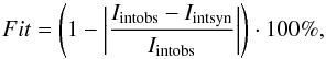 (5)where Iint means the value of integrated intensity for synthetic and observational profiles. As we can see in Table 3, for all brightenings, the fitting parameter is higher than 90%. The best result we got is for C brightening, the worst for the A event, which was easily predictable by taking into account the different emissions in the wings and the narrow wings. As mentioned in the previous section, integrated intensity represents the energy emitted within the line and it is not dependent, to some extent, e.g. on the plasma flows. Since we are not analysing the dynamics of CBs, we decided to used this parameter as a good representative of the physical conditions in the CBs. In the case of C and E events, we put two values of position, the first refers to the higher LTI, the second to the lowest. The same rule applies for temperature. Range of heights of the hotspot covers two LTIs, from the beginning of first to the end of the second. We notice some relationship between the shape of the profile and its position in the atmosphere, as mentioned above. A higher emission in the line peaks indicates a higher position of the hotspot in the atmosphere. Moreover, the more enhanced emission in the wings suggests the deeper position of the temperature increase. We can also claim that, even if the brightenings are formed at different positions, these heights are different only by about 400 km, which for the Sun-scale is not so great. It is clear that, generally, our brightenings are formed in the lower chromosphere to the upper photosphere, close to the temperature minimum region, which is in good agreement with the results of previous work (Berlicki & Heinzel 2014).
8. An effect of the overlying canopy
Arch filament systems are commonly overlying emerging flux regions and form a chromospheric canopy (Kitai 1983; Dara et al. 1997; Rutten et al. 2013). This canopy may have an important effect on the intensities in the cores of studied lines in CB/EBs. The canopy consists of many fine-structure elements that may extend to altitudes as high as a few thousands km and, indeed, may obscure the EB (see also recent study of Hong et al. 2014 based on classical cloud model). However, as already demonstrated in Heinzel & Schmieder (1994, see also references therein), these elements usually called mottles or fibrils may posses a range of temperatures and gas pressures that lead to the Hα line core contrast varying from absorption to emission. This is why Heinzel & Schmieder (1994) called them “black and white mottles”. In case of optically-thick lines like Mg II h and k, the line centre will thus exhibit the radiation of a mottle, while the peaks may result from a superposition of an attenuated radiation of EB and emission of the mottle itself. In the line wings we should see the EB’s and CB’s radiation unaffected by the canopy. In Fig. 3, we clearly see thin fibrils which may obscure some brightenings. Especially, CB A, C, and D seem to be overlaid by darker or brighter threads that are well visible in the Mg II h line centre.
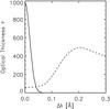 |
Fig. 11 Theoretical optical thickness τ of fibril within Mg II h line (solid line) calculated with 2D codes using our fibril model, and the theoretical Mg II h line profile for the CB C modified model 65-4 (dashed line) calculated using our NLTE chromospheric codes. The fibril model parameters are D = 2000 km, T = 10 000 K (isothermal), p = 2 dyn cm-2 (isobaric). The x scale is given in Å (0.1 Å corresponds to 4.5 km s-1). |
Simple consideration of the formal solution of the transfer equation shows that the spectral line profile emitted by CBs should be a composite of the fibril and CBs profiles: ![Mathematical equation: \begin{equation} I(\lambda) = I_{\rm CB}(\lambda) \exp[-\tau(\lambda)] + I_F(\lambda), \end{equation}](/articles/aa/full_html/2016/09/aa27358-15/aa27358-15-eq107.png) (6)where ICB is the emergent intensity of the CB modelled in this paper as a temperature perturbation of the C7 model, IF is the intensity of the fibril emergent from its top surface, and τ is the wavelength-dependent optical thickness of the fibril. We note that this formula represents a generalized cloud model with the variable line source function (classical cloud model of Beckers 1964 assumes a constant source function).
(6)where ICB is the emergent intensity of the CB modelled in this paper as a temperature perturbation of the C7 model, IF is the intensity of the fibril emergent from its top surface, and τ is the wavelength-dependent optical thickness of the fibril. We note that this formula represents a generalized cloud model with the variable line source function (classical cloud model of Beckers 1964 assumes a constant source function).
To estimate quantitatively the possible effects of the canopy, we performed preliminary NLTE modelling of fibrils that horizontally overlie the CBs. Fibrils are modelled as flux tubes with the cross-section much narrower compared to their length and for this geometry we apply a 2D radiative-transfer model. We considered a 2D rectangular box with af 2000 km width placed horizontally above the solar surface at an altitude of 5000 km (we note that the horizontal extension is infinite in the model). This structure is isothermal and isobaric and the box is illuminated by the solar disk radiation. We assumed the temperature of 1 × 10⁴ K and the pressure of 2 dyn/cm2. These values are based on previous studies of Heinzel et al. (1992), where the parameters of dark loops visible against the solar disk were discussed. At this altitude, the bottom of the box receives almost undiluted disk radiation, while both vertical sides are illuminated with the dilution factor of around one half. The top surface is not illuminated because the corona does not emit in Mg II lines. The thickness and the height of fibril was assumed according to the typical values obtained from observations. We adapted the 2D NLTE code described in Heinzel & Anzer (2001) and Heinzel et al. (2015) to compute the intensity of the fibril itself that was emergent from the top surface (e.g. as seen against the disk), and we also obtained the total optical thickness of the fibril over the line profile.
In Fig. 11 we see that the Mg II h line-centre optical thickness is enormous in the fibril and thus what we observe − provided that the CBs is obscured by the canopy − is the fibril radiation IF. However, it is very interesting to observe that at the location of the Mg II line peaks around 0.2 Å, the optical thickness of the fibril is already very small (τ ≈ 0.01), and thus the observed peaks indeed likely represent the radiation ICB of the CBs.
We note that by introducing flows in the fibril (typically of the order 10−20 km s-1 (see Heinzel & Schmieder 1994), we could account for the observed asymmetry of the peaks by the Doppler shift of the line-core absorption.
Our very preliminary tests showed that introducing a canopy fibril can explain the observed line centre intensities which depend on the fibril parameters. But the Mg II line peaks already represent the emission from the perturbed region of the quiet Sun atmosphere, i.e. the EBs or CBs. This conclusion is important in the case of the CB C profile: by introducing the overlying fibrils, this enbales a better fitting of the Mg II h line centre intensity. Since the observed line centre intensity of CB C is higher than in our theoretical profile, in this case the fibril should be in emission with respect to the surrounding chromosphere. In our next paper, we plan to perform systematic modelling of these types of fibrils, also including the flows, and compare the theoretical composite Mg II line profiles with the observed line spectra.
9. Discussion and conclusion
We have revisited the IRIS observations of the flux emergence of September 24, 2013 observed at 11:44 UT (Peter et al. 2014). We have also analysed the next raster starting at 15:39 UT to have a better statistics. The aim of the paper was to detect possible Ellerman bombs (EBs) in these two fields of view by using the Mg II spectra. EBs are well recognized in spectra of chromospheric lines (Hα and Ca II) by their so-called moustaches, with enhanced emission in the wings of the lines up to 10 Å. By way of an analogy, we investigated the wing intensities of Mg II lines, particularly Mg II h for practical reasons: the red wing of Mg II h is recorded along 4 Å and doesn’t overlap with the Mg II k line red wing. Using spectroheliograms reconstructed from the IRIS Mg II spectra, we identified 74 compact bright points (CBs) (38 and 36 respectively in each raster). They are mainly detected in the wings of the Mg II lines (at 1 Å and 3.5 Å). Only eight of them are also observed in the Mg II h2 peaks (at 0.23 Å). We classified the CBs by their contrasts in the peaks, in the wings, far wings, and quasi-continuum at 2830.4 Å in three categories (Table 2). The first type (the eight bright points) concerns bright points that have strong peak intensity and large contrast in the wings. These bright points belong to those that are clearly visible in Si IV lines and called “hot explosions” in Peter et al. (2014). We selected two of them and considered the more symmetrical profiles in the middle of each bomb (CBs A and B). The second type (CBs C and D) concerns the CBs that have large integrated intensities because of the large width of their profiles and not because of their peak intensities. They both have a strong signature in the Mg II triplet line that has a chromospheric formation temperature, just below the transition region temperature.
The third type of CBs (E), is an extreme case of type 2a in the spectra. The profile has very a low peak intensity and high intensity in the far wing and continuum. They have no signatures in Si IV and CII lines like CB (C).
Our main goal was to compute the formation height of these five examples of CBs (A to E) visible in Mg II lines. Therefore we applied the NLTE radiative transfer code used by Berlicki & Heinzel (2014) for Hα and Ca II lines to get synthetic Mg II line profiles to compare with the observations. The 1D atmosphere temperature profile is implemented with a hot temperature spot or local temperature increase (LTI) defined by a few parameters, such as the position, the width, and the amplitude. The density value is fixed because the model is relatively insensitive to density variations (Berlicki & Heinzel 2014). We computed a grid of models and a grid of the corresponding Mg II and Hα synthetic profiles.
We have used an automatic detection method that is based on the parameters determined for each type of Mg II h profiles and then refined the search by visual inspection to fit the observed profiles with synthetic profiles. Five CB models were computed, one for each CB (A to E) with one or two hotspots in the temperature profile. The hotspots are located in the photosphere between 75 km to 300 km and, for some of them, reached the chromosphere up to 900 km. According to our statistics, 80% of the CBs have a type between C and E, the profiles are relatively well fitted with an extended hotspot with two peaks at a distance of 700 km reaching two different temperatures around 6200 K and about 7350 K. The increase of temperature reaches 3350 degrees. However the centre of the line h3 is generally higher than the h3 of the QS. This can be the effect of the overlying fibrils. To test this effect, we have used a 2D NLTE static model of fibrils. We show that this model can increase h3 in the observed proportion, but does not affect the h2 peaks of the Mg II h line profile.
The question about the existence of EBs in Mg II h and k lines is important. EBs are mainly defined by the Hα line profiles. To be sure about the properties of EBs in Mg II h and k lines we need simultaneous observations in Hα, as in the papers of Vissers et al. (2015) and Kim et al. (2015). Our observation of AR11850 in Hα is from the same day, but not simultaneous. Therefore they cannot be used directly. We attempt the comparison with our theoretical models and derived the synthetic profiles of Hα for the five CB models A to E (colour profiles in Fig. 2). The Hα synthetic profiles are consistent either with Hα THEMIS profiles (CB E) (black profile in Fig. 2) and/or with those obtained with the SST/CRISP and the NST (Vissers et al. 2015; Kim et al. 2015). The wings of the Hα C profile have enhanced intensities up to 25% in Hα +/−2 Å similar to the EBs of the NST (see the Fig. 5 in Kim et al. 2015) and up to 50% at Hα− 1.25 Å as for EB1 (see Fig. 4 in Vissers et al. 2015).
A discussion on the type 1 and type 2b of CBs that have signatures in Si IV and CII lines show that these CBs are comparable to the hot explosions observed in Peter et al. (2014; their bombs 3 and 4 correspond to CBs A and B). Their corresponding Hα synthetic profiles obtained with these two CB types using our CB models (models A, B, and C) correspond to the profiles of EB1 and EB2 observed by Vissers et al. (2015; see their Figs. 4 and 8 top left panel) who found associated Hα EBs in the field of view of SST. The CB D profile is closer to the profile FAF1 of Vissers et al. (2015; see their Fig. 13, top left panel) and can correspond to EBs overlaid by AFS. The test of the 2D model of the fibril was not done on this profile whose intensity and shape are far from being a classical Mg II profile. This should be done in a more extensive study on the influence of overlying fibrils.
To conclude, the three types of Mg II profiles could correspond to EBs. The reconnection seems to occur in the low atmosphere and could correspond to some plasmoid instability (Ni et al. 2015). The fast evolution of the bidirectional flows observed in hot lines (Si IV and C II) correlated with a weak EB would correspond more to a fast reconnection in the upper atmosphere (Kim et al. 2015). The model of reconnection in the corona of Archontis & Hansteen (2014) in this way is a promising simulation to explain the type of explosive events observed in Si IV lines, but their model cannot really explain the formation of simultaneous Hα EBs, which requires a reconnection in the photosphere. In the paper of Dudík et al. (2014), there is interesting information about the temperature of the formation of Si IV lines in a non-Maxwellian distribution of electrons. With a κ distribution, the temperature of the formation of Si IV can be just a chromospheric temperature and the intensity of the O IV line would be reduced, which could also explain the absence of signature of O IV in the hot explosions of Peter et al. (2014). An alternative to this scenario has been proposed by Judge (2015), taking into consideration the existence of Alfvénic turbulence in the plasma. The mechanisms of the formation of EBs are likely even more complex than was thought. This topic is very open. A further diagnostic of the physical properties from the line profile should help us determine the conditions in the atmosphere (Leenaarts et al. 2013b).
Acknowledgments
We would like to thank the anonymous referee who helped us to bring the manuscript to the acceptation stage owing to his/her helpful comments. We want to thank Bernard Gelly, the director of THEMIS and his colleagues for the observations with THEMIS/MTR instrument, to thank the observers of the Meudon solar tower (Regis Lecocguen and Daniel Crussaire) for the MSDP data. We thank Nicole Mein for the MSDP data reduction and the coalignement of the MSDP images with the IRIS images. We thank Liu Tian who provided us with the additional IRIS software that he had personally developed and Véronique Bommier for the THEMIS interface software, which we used for getting the Hα line profiles. This work is partially supported by the European Community Seventh Framework Programme (FP7/2007−2013) under grant agreement No. 606862 (F-CHROMA), by the grant of Polish Ministry of Sciences and Higher Education No. 3243/7.PR/14/2015/2 (2014−2016), by the grant No. 16-18495S of the Grant Agency of the Czech Republic and by the institutional grant RVO 67985815. IRIS is a NASA small explorer mission developed and operated by LMSAL with mission operations executed at NASA Ames Research Center and major contributions to downlink communications funded by ESA and the Norwegian Space Centre. The National Center for Atmospheric Research is sponsored by the National Science Foundation. We thank ISSI (Bern) for the workshop on “UV burst” managed by P. Young, which helped us to clarify our studies on the relationship between UB bursts and Ellerman bombs.
References
- Archontis, V., & Hansteen, V. 2014, ApJ, 788, L2 [NASA ADS] [CrossRef] [Google Scholar]
- Archontis, V., & Hood, A. W. 2009, A&A, 508, 1469 [NASA ADS] [CrossRef] [EDP Sciences] [Google Scholar]
- Avrett, E. H., & Loeser, R. 2008, ApJS, 175, 229 [NASA ADS] [CrossRef] [Google Scholar]
- Beckers, J. M. 1964, Ph.D. Thesis, Sacramento Peak Observatory, Air Force Cambridge Research Laboratories, Mass., USA [Google Scholar]
- Berlicki, A., & Heinzel, P. 2014, A&A, 567, A110 [NASA ADS] [CrossRef] [EDP Sciences] [Google Scholar]
- Berlicki, A., Heinzel, P., Schmieder, B., Mein, P., & Mein, N. 2005, A&A, 430, 679 [NASA ADS] [CrossRef] [EDP Sciences] [Google Scholar]
- Bernasconi, P. N., Rust, D. M., Georgoulis, M. K., & Labonte, B. J. 2002, Sol. Phys., 209, 119 [NASA ADS] [CrossRef] [Google Scholar]
- Cheung, M. C. M., Schüssler, M., Tarbell, T. D., & Title, A. M. 2008, ApJ, 687, 1373 [NASA ADS] [CrossRef] [Google Scholar]
- Dara, H. C., Alissandrakis, C. E., Zachariadis, T. G., & Georgakilas, A. A. 1997, A&A, 322, 653 [NASA ADS] [Google Scholar]
- David, K.-H. 1961, Z. Astrophys., 53, 37 [NASA ADS] [Google Scholar]
- De Pontieu, B., Title, A. M., Lemen, J. R., et al. 2014, Sol. Phys., 289, 2733 [NASA ADS] [CrossRef] [Google Scholar]
- Dudík, J., Del Zanna, G., Dzifčáková, E., Mason, H. E., & Golub, L. 2014, ApJ, 780, L12 [NASA ADS] [CrossRef] [Google Scholar]
- Dumont, S. 1967, Ann. Astrophys., 30, 861 [NASA ADS] [Google Scholar]
- Ellerman, F. 1917, ApJ, 46, 298 [NASA ADS] [CrossRef] [Google Scholar]
- Fang, C., Tang, Y. H., Xu, Z., Ding, M. D., & Chen, P. F. 2006, ApJ, 643, 1325 [NASA ADS] [CrossRef] [Google Scholar]
- Georgoulis, M. K., Rust, D. M., Bernasconi, P. N., & Schmieder, B. 2002, ApJ, 575, 506 [NASA ADS] [CrossRef] [Google Scholar]
- Hashimoto, Y., Kitai, R., Ichimoto, K., et al. 2010, PASJ, 62, 879 [NASA ADS] [Google Scholar]
- Heinzel, P. 1995, A&A, 299, 563 [NASA ADS] [Google Scholar]
- Heinzel, P., & Anzer, U. 2001, A&A, 375, 1082 [NASA ADS] [CrossRef] [EDP Sciences] [Google Scholar]
- Heinzel, P., & Schmieder, B. 1994, A&A, 282, 939 [NASA ADS] [Google Scholar]
- Heinzel, P., Schmieder, B., & Mein, P. 1992, Sol. Phys., 139, 81 [NASA ADS] [CrossRef] [Google Scholar]
- Heinzel, P., Schmieder, B., Mein, N., & Gunár, S. 2015, ApJ, 800, L13 [NASA ADS] [CrossRef] [Google Scholar]
- Herlender, M., & Berlicki, A. 2011, Central European Astrophysical Bulletin, 35, 181 [Google Scholar]
- Hong, J., Ding, M. D., Li, Y., Fang, C., & Cao, W. 2014, ApJ, 792, 13 [NASA ADS] [CrossRef] [Google Scholar]
- Isobe, H., Tripathi, D., & Archontis, V. 2007, ApJ, 657, L53 [NASA ADS] [CrossRef] [Google Scholar]
- Judge, P. G. 2015, ApJ, 808, 116 [NASA ADS] [CrossRef] [Google Scholar]
- Kim, Y.-H., Yurchyshyn, V., Bong, S.-C., et al. 2015, ApJ, 810, 38 [NASA ADS] [CrossRef] [Google Scholar]
- Kitai, R. 1983, Sol. Phys., 87, 135 [NASA ADS] [CrossRef] [Google Scholar]
- Leenaarts, J., Pereira, T. M. D., Carlsson, M., Uitenbroek, H., & De Pontieu, B. 2013a, ApJ, 772, 89 [NASA ADS] [CrossRef] [Google Scholar]
- Leenaarts, J., Pereira, T. M. D., Carlsson, M., Uitenbroek, H., & De Pontieu, B. 2013b, ApJ, 772, 90 [NASA ADS] [CrossRef] [Google Scholar]
- López Ariste, A., Rayrole, J., & Semel, M. 2000, A&AS, 142, 137 [NASA ADS] [CrossRef] [EDP Sciences] [Google Scholar]
- Matsumoto, T., Kitai, R., Shibata, K., et al. 2008, PASJ, 60, 95 [NASA ADS] [Google Scholar]
- Mein, P., & Mein, N. 1988, A&A, 203, 162 [NASA ADS] [Google Scholar]
- Milkey, R. W., & Mihalas, D. 1974, ApJ, 192, 769 [NASA ADS] [CrossRef] [Google Scholar]
- Nelson, C. J., Doyle, J. G., Erdélyi, R., et al. 2013a, Sol. Phys., 283, 307 [NASA ADS] [CrossRef] [Google Scholar]
- Nelson, C. J., Shelyag, S., Mathioudakis, M., et al. 2013b, ApJ, 779, 125 [NASA ADS] [CrossRef] [Google Scholar]
- Nelson, C. J., Scullion, E. M., Doyle, J. G., Freij, N., & Erdélyi, R. 2015, ApJ, 798, 19 [NASA ADS] [CrossRef] [Google Scholar]
- Ni, L., Kliem, B., Lin, J., & Wu, N. 2015, ApJ, 799, 79 [NASA ADS] [CrossRef] [Google Scholar]
- Pariat, E., Aulanier, G., Schmieder, B., et al. 2004, ApJ, 614, 1099 [Google Scholar]
- Pariat, E., Schmieder, B., Berlicki, A., et al. 2007, A&A, 473, 279 [NASA ADS] [CrossRef] [EDP Sciences] [Google Scholar]
- Pariat, E., Masson, S., & Aulanier, G. 2009, ApJ, 701, 1911 [NASA ADS] [CrossRef] [Google Scholar]
- Pereira, T. M. D., Leenaarts, J., De Pontieu, B., Carlsson, M., & Uitenbroek, H. 2013, ApJ, 778, 143 [NASA ADS] [CrossRef] [Google Scholar]
- Peter, H., Tian, H., Curdt, W., et al. 2014, Science, 346, 1255726 [NASA ADS] [CrossRef] [Google Scholar]
- Rutten, R. J., Vissers, G. J. M., Rouppe van der Voort, L. H. M., Sütterlin, P., & Vitas, N. 2013, J. Phys. Conf. Ser., 440, 012007 [NASA ADS] [CrossRef] [Google Scholar]
- Rybicki, G. B., & Hummer, D. G. 1991, A&A, 245, 171 [NASA ADS] [Google Scholar]
- Rybicki, G. B., & Hummer, D. G. 1992, A&A, 262, 209 [NASA ADS] [Google Scholar]
- Sandlin, G. D., Bartoe, J.-D. F., Brueckner, G. E., Tousey, R., & Vanhoosier, M. E. 1986, ApJS, 61, 801 [NASA ADS] [CrossRef] [Google Scholar]
- Schmieder, B., Rust, D. M., Georgoulis, M. K., Démoulin, P., & Bernasconi, P. N. 2004, ApJ, 601, 530 [NASA ADS] [CrossRef] [Google Scholar]
- Schmieder, B., Archontis, V., & Pariat, E. 2014, Space Sci. Rev., 186, 227 [NASA ADS] [CrossRef] [Google Scholar]
- Shine, R. A., & Linsky, J. L. 1974, Sol. Phys., 39, 49 [NASA ADS] [CrossRef] [Google Scholar]
- Socas-Navarro, H., Martínez Pillet, V., Elmore, D., et al. 2006, Sol. Phys., 235, 75 [NASA ADS] [CrossRef] [Google Scholar]
- Staath, E., & Lemaire, P. 1995, A&A, 295, 517 [NASA ADS] [Google Scholar]
- Tian, H., Xu, Z., He, J., & Madsen, C. 2016, ApJ, 824, 96 [NASA ADS] [CrossRef] [Google Scholar]
- Vissers, G. J. M., Rouppe van der Voort, L. H. M., & Rutten, R. J. 2013, ApJ, 774, 32 [NASA ADS] [CrossRef] [Google Scholar]
- Vissers, G. J. M., Rouppe van der Voort, L. H. M., Rutten, R. J., Carlsson, M., & De Pontieu, B. 2015, ApJ, 812, 11 [NASA ADS] [CrossRef] [Google Scholar]
- Watanabe, H., Kitai, R., Okamoto, K., et al. 2008, ApJ, 684, 736 [NASA ADS] [CrossRef] [Google Scholar]
- Watanabe, H., Vissers, G., Kitai, R., Rouppe van der Voort, L., & Rutten, R. J. 2011, ApJ, 736, 71 [NASA ADS] [CrossRef] [Google Scholar]
- Xu, X.-Y., Fang, C., Ding, M.-D., & Gao, D.-H. 2011, RA&A, 11, 225 [Google Scholar]
All Tables
IRIS lines of interest (rest wavelengths from the line list of Sandlin et al. 1986).
All Figures
|
Fig. 1 Active region AR 11850 observed on September 24, 2013 from left to right: full disk image in AIA 304 Å, the white box indicates the field of view of the two right panels (140 × 175 arcsec2), Hα image (MSDP/Meudon spectrograph) and Mg II k line centre at 2803.5 Å obtained between 11:43 and 12:04 UT (IRIS spectrograph) showing the arch filament system (AFS). The two white boxes in the IRIS panel represent the field of view of the two small rasters presented in Figs. 3 and 4. |
| In the text | |
|
Fig. 2 Top panel: spectrum of an EB in H α line observed by THEMIS/MTR spectropolarimeter. The two red arrows indicate the EB in I+V and I-V channels. Bottom panel: Hα profiles – Observed profiles: EB profile of the THEMIS spectrum shown in the top panel (solid black line), observed nearby quiet Sun profile from THEMIS (thin black line). Synthetic profiles computed from NLTE modelling: QS (purple solid line). All colour profiles described with letters from A to E are calculated for each best model of selected CBs (A − red; B − orange; C − light green; D − light blue; E − dark blue). Intensity units is (erg s-1 cm -2 Å-1sr-1), Δλ unit is Å. |
| In the text | |
|
Fig. 3 AR 11850 IRIS observations of raster 1 (the field of view is indicated in Fig. 1, right panel). Top and middle panels from left to right: Mg II spectroheliograms at 2800.0 Å, 2803.5 Å, 2803.7 Å and 2804.5 Å. Bottom left panel: spectroheliogram in the continuum at 2831.1 Å. Bottom right panel: spectroheliogram in Si V line. White or dark boxes show the selected CBs from A to D (the numbers in parenthesis indicate the hot explosions of Peter et al. 2014), small white circles with numbers 5 to 9 in the second row, right panel are examples of small brightenings. |
| In the text | |
|
Fig. 4 AR 11850 IRIS observations of raster 2 (the field of view is indicated in Fig. 1, right panel). Top and middle panels from left to right: Mg II spectroheliograms at 2800.0 Å, 2803.5 Å, 2803.7 Å, and 2804.5 Å. Bottom left panel: spectroheliogram in Si IV line. Black circles in Mg II +0.1 Å and in Si IV spectroheliogram indicate CBs visible in Si IV and Mg II line wing. Bottom right panel: slit-jaw image at 2796 Å. The white box indicates the location of the CB (E) that we have analysed. The EB (E) is not visible in Si IV and Mg II core of the line. |
| In the text | |
|
Fig. 5 Spectra and profiles of Mg II h and k and Mg II triplet at 2798.7 Å lines for the five selected CBs. Two top rows: spectra of the CBs shown in the boxes of Figs. 3 and 4. The arrows indicate the positions of each CB: A to E at y = 47.5, 59.0, 50.9, 52.7, 74.2 arcsec, respectively, where the profiles are taken and drawn below. Bottom five plots: profiles of A to E (solid line) with the QS (dotted line) and the nearby quiet profile (dashed thin line). Bottom right panel: plot of all the selected profiles shown in a different colour: A − purple; B − green; C − blue; D − red; and E − black. Intensity units is (erg s-1 cm -2Å-1sr-1), wavelengths unit is Å. For CBs C and D, we note that the emission of Mg II triplet is enhanced and its line profile is absorbed by an Mg II line (2798.6 Å) in the blue wing and by an Mn I line (2799.2 Å) in the red wing. |
| In the text | |
|
Fig. 6 Four top rows: spectra of Si IV 1394 Å , Si IV 1403 Å, and C II 1336 Å of the five selected A to E CBs. Bottom left and right panels: example of multi structures in CBs along the slit: Mg II h and Si IV 1394 Å respectively profiles in the CB B: B1 identical to B for y = 59 arcsec (pixel = 374) (solid line), B2 for y = 59−0.33 arcsec (pixel = 372) (dashed line), B3 for y = 59 + 0.5 arcsec (pixel = 377) (dashed-dotted-dotted line), with profiles outside the bomb (y = 61.5 arcsec (pixel = 389) − dashed-dotted line). The bright spectra with a large blue shift below B is not considered as belonging to CB B. The Si IV 1393.76 line blue wing is ragged by two absorption lines (Fe II at 1392.2 Å) and Ni II (1393.3 Å) for CBs A B, and D. Intensity units are in (erg s-1 cm -2Å-1sr-1), wavelengths unit is Å. |
| In the text | |
|
Fig. 7 Intensity profiles of Mg II lines for events that have high intensity in the wings and small intensity in the peaks. The selection was done randomly (see the small circles in Fig. 3). The correspondence is as follows: 5 − dark blue; 6 − light blue; 7 − red; 8 − orange; 9 − light green. The black line represents the E profile. All these profiles have a shape between CB C and CB E profiles. |
| In the text | |
|
Fig. 8 Examples of synthetic profiles for different models: chromospheric 53-5, model of the hotspot in low chromosphere, close to the temperature minimum region 65-7 and photospheric model 77-6. For each model a different part of the profiles is enhanced. |
| In the text | |
|
Fig. 9 Left panel: example of one profile parameter, such as the right integrated intensity obtained for all models. The horizontal lines on the diagram represent the values of the parameter for the observed profiles − dotted line for A brightening, dashed line for B, dashed dotted line C, dashed-dotted-dotted-dotted for D and long dashed line for E. Right panel: the square root of the mean-square intensity difference between synthetic and observed profiles: one example of the A brightening. The best model for A is N = 120. |
| In the text | |
|
Fig. 10 Plots with the results of modelling. The first two left columns show some synthetic profiles (solid line) compared with observational profiles (dashed line) for best models from the grid. Some of the profiles are chosen from method based on profiles parameters, some of them have additional profile chosen after visual verification (63-5 for B, 73-1 for C, 68-4 for D, 75-1 for E). The third column presents the synthetic profiles (solid line) obtained from modified models compared with observational profiles (dashed line). In the last, right column, we present the temperature structure of the best models plotted with a black solid line. The dashed line represents models before modification. In this figure, each row corresponds to other compact brightening from A to E, respectively. |
| In the text | |
|
Fig. 11 Theoretical optical thickness τ of fibril within Mg II h line (solid line) calculated with 2D codes using our fibril model, and the theoretical Mg II h line profile for the CB C modified model 65-4 (dashed line) calculated using our NLTE chromospheric codes. The fibril model parameters are D = 2000 km, T = 10 000 K (isothermal), p = 2 dyn cm-2 (isobaric). The x scale is given in Å (0.1 Å corresponds to 4.5 km s-1). |
| In the text | |
Current usage metrics show cumulative count of Article Views (full-text article views including HTML views, PDF and ePub downloads, according to the available data) and Abstracts Views on Vision4Press platform.
Data correspond to usage on the plateform after 2015. The current usage metrics is available 48-96 hours after online publication and is updated daily on week days.
Initial download of the metrics may take a while.