| Issue |
A&A
Volume 593, September 2016
|
|
|---|---|---|
| Article Number | A122 | |
| Number of page(s) | 13 | |
| Section | Extragalactic astronomy | |
| DOI | https://doi.org/10.1051/0004-6361/201527024 | |
| Published online | 04 October 2016 | |
Lyman-α blobs: polarization arising from cold accretion
1 Univ. Lyon, Univ. Lyon1, ENS de Lyon, CNRS, Centre de Recherche Astrophysique de Lyon, UMR 5574, 69230 Saint-Genis-Laval, France
e-mail: This email address is being protected from spambots. You need JavaScript enabled to view it.
2 Observatoire de Genève, Université de Genève, 51 Ch. des Maillettes, 1290 Sauverny, Switzerland
3 Leiden Observatory, Leiden University, PO Box 9513, 2300 RA Leiden, The Netherlands
Received: 21 July 2015
Accepted: 5 April 2016
Abstract
Lyman-α nebulae are typically found in massive environments at high redshift (z ≳ 2). The origin of their Lyman-α (Lyα) emission remains debated. Recent polarimetric observations showed that at least some Lyα sources are polarized. This is often interpreted as proof that the photons are centrally produced and contradicts the scenario in which the Lyα emission is the cooling radiation emitted by gas that is heated during the accretion onto the halo. We suggest that this cooling radiation scenario is compatible with the polarimetric observations. To test this idea, we post-processed a radiative hydrodynamics simulation of a blob with the MCLya Monte Carlo transfer code. We computed radial profiles for the surface brightness and the degree of polarization and compared them to existing observations. We found that computed and observed profiles both are consistent with a significant contribution of the extragalactic gas to the Lyα emission. Most of the photons are centrally emitted and are subsequently scattered inside the filament, which produces the observed high level of polarization. We argue that the contribution of the extragalactic gas to the Lyα emission does not prevent polarization. On the contrary, we find that pure galactic emission causes the polarization profile to be too steep to be consistent with observations.
Key words: scattering / polarization / diffusion / intergalactic medium / galaxies: high-redshift / methods: numerical
© ESO, 2016
1. Introduction
Spatially extended high-redshift (z ≳ 2) Lyman-α nebulae (HzLAN) were discovered more than twenty years ago by Chambers et al. (1990) and have since been regularly observed around powerful radio sources (Heckman et al. 1991; van Ojik et al. 1997; Villar-Martín et al. 2002, 2007; Reuland et al. 2003). In the early 2000s, Steidel et al. (2000, but see also Francis et al. 1996, Fynbo et al. 1999, Keel et al. 1999 found similar objects at z ≃ 3 that were not associated with radio galaxies. Their physical properties are very similar to the HzLANs previously found, with sizes of up to a few hundred kilo-parsecs, and Lyα luminosities of up to 1044 erg s-1. A few hundred of these HzLANs (called Lyman-α blobs or LABs) have been found at z = 2−6.5 by recent surveys (Palunas et al. 2004; Matsuda et al. 2004, 2006; Dey et al. 2005; Saito et al. 2006; Ouchi et al. 2009; Yang et al. 2009, 2010; Prescott et al. 2013). They are usually associated with quasars (Bunker et al. 2003; Basu-Zych & Scharf 2004; Weidinger et al. 2004; Christensen et al. 2006; Scarlata et al. 2009; Smith et al. 2009; Overzier et al. 2013), Lyman-break galaxies (Matsuda et al. 2004), and infrared or sub-millimetre sources (Chapman et al. 2001; Dey et al. 2005; Geach et al. 2005, 2007, 2014; Matsuda et al. 2007). For some of these LABs, no galactic counterpart has been found (Nilsson et al. 2006, see also blob 6 of Erb et al. 2011). All these associations support the consensus that HzLANs are located in massive haloes in the densest regions of the Universe (Steidel et al. 2000; Matsuda et al. 2004, 2006; Prescott et al. 2008; Saito et al. 2015).
These observations raise two fundamental questions: where do the vast quantities of emitting gas come from, and which sources of energy power the observed Lyα emission? It has become clear during the past decade that a significant fraction of the gas in massive haloes at high redshifts is cold (see e.g. Birnboim & Dekel 2003; Kereš et al. 2005; Dekel & Birnboim 2006; Ocvirk et al. 2008; Brooks et al. 2009; Kereš et al. 2009; van de Voort et al. 2011; van de Voort & Schaye 2012). Simulations suggest that this cold gas reservoir is a complex mixture, dominated in mass by primordial accretion streams and tidal streams from galaxy interactions, and that it is probably this gas that we see shine in HzLANs. The second question remains largely open, however, and it is unclear which energy source triggers (or sustains) Lyα emission in this gas. There are basically three scenarios. The Lyα radiation may be due to rapid cooling following shock-heating of this gas by large galactic outflows (e.g. Taniguchi & Shioya 2000; Ohyama et al. 2003; Mori et al. 2004; Geach et al. 2005). Alternatively, the Lyα radiation may be emitted by recombinations that follow photo-ionization from the intergalactic ultraviolet background (Gould & Weinberg 1996) or from local sources (Haiman & Rees 2001; Cantalupo et al. 2005, 2014; Kollmeier et al. 2010). Finally, the Lyα radiation may trace the dissipation of gravitational energy through collisional excitations as gas falls towards galaxies (Haiman et al. 2000; Fardal et al. 2001; Furlanetto et al. 2005; Dijkstra et al. 2006; Dijkstra & Loeb 2009; Faucher-Giguère et al. 2010; Goerdt et al. 2010; Rosdahl & Blaizot 2012). We emphasize that the cold stream scenario has been suggested in response to the broad variety of sources LABs are associated with. It provides a single mechanism to explain the Lyα radiation for this variety of sources, without relying on an active galactic nucleus (AGN), for instance, that is associated with the blob (see Dijkstra & Loeb 2009). This latter scenario, often dubbed the cold stream scenario, is the focus of the present paper.
Because simulations that describe any of these three possible contributions to the luminosity of HzLANs are so uncertain, it would be preferable to find observables that might help separate them observationally. It has been shown that scattering may lead to a polarized Lyα emission around high-redshift galaxies and collapsing haloes (Lee & Ahn 1998; Rybicki & Loeb 1999; Dijkstra & Loeb 2008), and the degree of polarization of HzLANs may indeed help us distinguish the emission processes. In particular, it was argued by Dijkstra & Loeb (2009) that emission from cold accretion streams would not produce a polarized signal structured at the scale of the blob because of the small volume filling of such streams. The first positive observation by Hayes et al. (2011, hereafter H11 of linear polarization forming a large-scale ring pattern around the Lyα peak of LAB1 (Steidel et al. 2000) was interpreted as a strong argument against the cold stream scenario. Humphrey et al. (2013) also found the same level of polarization around the radio galaxy TXS 0211-122. Earlier observations from Prescott et al. (2011) showed no evidence for polarization around the HzLAN LABd05, but H11 argued that this was due to a too low signal-to-noise ratio.
In the present paper, we revisit the question of the polarization of HzLANs from a theoretical perspective. We wish to test whether the results of Dijkstra & Loeb (2008, hereafter DL08, for example, which were based on idealised geometrical configurations, hold when the full complexity of the cosmological context is taken into account. This will allow us to provide an alternative key to interpret polarization constraints that takes this complexity into account. We do this by extending the work of Rosdahl & Blaizot (2012, hereafter RB12 to assess whether their most recent simulation of a typical LAB (their halo H2, of mass ~ 1012 M⊙ at z = 3) is compatible with the observations of H11. We show that this is the case and then use it to discuss the composite origin of the polarization feature H11 observed.
In Sect. 2 we present the details of the simulation of RB12 that we use and describe our new version of the Monte Carlo radiative transfer code MCLya (Verhamme et al. 2006), which now tracks polarization of Lyα photons. We then discuss in detail how we sampled the emission from gas and stars in the simulation, and how we built polarization maps from the results of MCLya. In Sect. 3 we present our results and compare them to observations of H11. We then discuss the origin of the polarization signal in our simulated nebula. Finally, we conclude in Sect. 4.
2. Method
2.1. Description of the RHD simulation
This work is based on the H2 simulation taken from RB12, which is our best model for a typical giant LAB at redshift 3. This simulation describes a halo of ~ 1012 M⊙ at z ~ 3, which is a group of galaxies penetrated by cold accretion streams. We refer to RB12 for a full description of the numerical details and a discussion of the physical processes at play in this halo.
In short, this simulation was performed with Ramses-RT (Rosdahl et al. 2013), a modified version of the adaptive mesh refinement (AMR) code Ramses (Teyssier 2002), which couples radiative transfer of ultraviolet photons to the hydrodynamics. This radiation hydrodynamics (RHD) method allows to follow accurately the ionisation and thermal state of the intergalactic and circumgalactic media (IGM, CGM), accounting for self-shielding of the gas against the UV background. The Lyα emissivity of the gas can be accurately computed based on this (see discussions in Faucher-Giguère et al. 2010; Rosdahl & Blaizot 2012). We used a zoom technique to achieve a resolution of up to 434 pc at z = 3, with a dark matter mass resolution of 1.1 × 10⁷ M⊙. We note that the refinement criteria we chose are such that the highest resolution is not only reached in the high-density ISM, but also along the cold streams.
For the analysis below, we define the star-forming interstellar medium (ISM) as gas denser than nH ≥ 0.76 cm-3, the CGM as gas at density 0.23 cm-3 ≤ nH < 0.76 cm-3, and the accretion streams as 0.015 cm-3 ≤ nH < 0.23 cm-3. We refer to the gas with lower density as diffuse gas. We note that these selections, although they rely on density alone (and not temperature), clearly select cold streams. This is probably partly due to the relative simplicity of the CGM in our simulation, which does not include feedback from supernovae.
2.2. Polarized Lyα radiative transfer: MCLYA
The simulated halo H2 described in Sect. 2.1 was post-processed using an improved version of the Monte Carlo Lyα transfer code, MCLya (Verhamme et al. 2006). Most of the improvements have been discussed in Verhamme et al. (2012): MCLya now makes use of the AMR structure of Ramses and includes more detailed physics for the Lyα line. The new version of the code we used here introduces the ability to propagate photons emitted by the gas (see Sect. 2.3), and most importantly, to track the polarization state of Monte Carlo photons.
As pointed out by DL08, the precise atomic level involved in the scattering of a Lyα photon is strongly correlated with the scattering phase function: the 1S1 / 2 → 2P1 / 2 → 1S1 / 2 (K transition) scattering sequence is described by an isotropic phase function, which means that any polarization information is lost. In contrast, the 1S1 / 2 → 2P3 / 2 → 1S1 / 2 (H transition) sequence retains a memory of the pre-scattering state of the photon. Hamilton (1947) showed that when they occur close enough to line centre (i.e. in the core), H transitions are well described by a superposition of an isotropic phase function and a Rayleigh phase function, with equal weights. Stenflo (1980) later showed that for a scattering event outside of the Lyα line centre (i.e. in the wings), the two transitions H and K interfere, and the event can instead be described by a single Rayleigh phase function. A convenient way to express the frequency is through its Doppler shift with respect to the Lyα line centre, x = (ν−νLyα) / ΔνD, where ΔνD = (vth + vturb)νLyα/c. In this formula, νLyα = 2.466 Hz (λLyα = 1215.668 Å) is the Lyα line frequency, vth is the thermal velocity of hydrogen atoms, vturb is a turbulent velocity, describing the small-scale turbulence of the gas, and c is the speed of light. Dijkstra & Loeb (2008, Appendix A2) showed that when we compute the photon frequency in the frame of the atom involved in the scattering event in a Monte Carlo simulation, we can take xcrit ≃ 0.2 to separate these two regimes of the H transition (core and wings). We follow their recommendation in the present paper, as we discuss below in this section.
There are mainly two approaches to describe the polarization state of light in a Monte Carlo framework. One possibility would be to consider groups of photons and compute the Stokes vector after each interaction as the result of a multiplication with a scattering matrix (Code & Whitney 1995; Whitney 2011). The other possibility is to use the technique described by Rybicki & Loeb (1999), which is the one we implemented in this paper. In this formalism, each Monte Carlo photon has a 100% linear polarization given by a unit vector e orthogonal to the propagation direction n of the photon: e·n = 0. The observed Stokes parameters will arise from the sum of multiple, independent MC photons. Their initial scheme is only valid for a Rayleigh scattering event, but can be easily modified to take resonant scattering into account, since resonant scattering is described by a superposition of Rayleigh and isotropic scattering.
For scattering events in the line core, the probability of a K transition is 1 / 3 and 2 / 3 for an H transition. The H transition is described by 50% of Rayleigh scattering and 50% of isotropic scattering, and a K transition always corresponds to an isotropic scattering. This implies that for core photons (with | x | < 0.2 in the atom frame) 2 / 3 of the scattering events are actually isotropic (i.e. lose polarization), while 1 / 3 are Rayleigh scatterings. For wing photons (| x | > 0.2), all scatterings are Rayleigh scatterings.
For an isotropic scattering event, the direction of propagation after scattering n′ and the new direction of polarization e′ are both randomly generated: n′ is uniformly drawn on a sphere, and e′ is uniformly drawn on a unit circle in a plane orthogonal to n′.
For a Rayleigh scattering event, it can be shown (see for instance Dijkstra & Loeb 2008, Appendix A3; also Rybicki & Loeb 1999) that the phase function can be simulated using a rejection technique: a random direction n′ and a random number R ∈ [0,1 [ are drawn, and the new direction is accepted if R< 1−(e·n′)2. Otherwise, a new direction and a new number are drawn again. The new polarization vector e′ is given by the projection of the previous polarization vector e on the plane normal to n′: 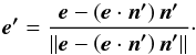 (1)
(1)
2.3. Lyα sources
One of the motivations of this work is to understand whether polarimetric observation can be a tool to elucidate the origin of the Lyα emission of blobs (extended or centrally concentrated). We decomposed the total Lyα emission into two components: the extragalactic part is emitted by gas at densities nH ≤ 0.76 cm-3 and is therefore composed of CGM, cold streams, and more diffuse gas, and the galactic part corresponds to the photons emitted by galaxies, that is, form material at densities nH ≥ 0.76 cm-3.
In our transfer code, a Monte Carlo photon is defined by a few quantities: position, propagation and polarization directions, luminosity, and frequency. The initial propagation direction of a photon is randomly drawn on a sphere. This defines the initial polarization plane, in which lies the polarization direction (which is randomly drawn on a circle). The initial positions, luminosity, and frequency of a photon are source-dependent. For the extragalactic emission, the photons are emitted directly from the simulation cells, and the luminosity and frequency is computed from the gas properties (see Sect. 2.3.3). For the galactic emission, we used the star particles from the simulation as a proxy for the Lyα sources. Their luminosities and frequencies are computed as explained in Sect. 2.3.2.
2.3.1. Lyman-α emission processes
Lyα emission is generated by two channels: collisional excitation of a hydrogen atom, and recombination of a free electron on a H ii ion.
The collisional mechanism is the following: a free electron excites an H i atom, which can relax to its ground state. During its radiative cascade, a 2P → 1S transition may occur, causing the emission of a Lyα photon. We approximate the collisional emissivity with  (2)where ne and nH i are the electron and H i number densities, ϵLyα = 10.2eV is the Lyα photon energy, and CLyα(T) is the rate of collisionally induced 1S → 2P transitions. We used the expression given by Goerdt et al. (2010) for CLyα(T), fitting the results from Callaway et al. (1987).
The recombination process occurs when a free electron recombines with a proton to give an excited hydrogen atom. This atom may cascade down to the 2P level from its excited state, eventually relaxing to the ground state and producing a Lyα photon. The Lyα emissivity of the process is given by  (3)where the 0.68-factor is the average number of Lyα photon produced for each recombination, assuming case B and a typical gas temperature of 104 K (Osterbrock & Ferland 2006), nH ii is the proton number density, and
  is the case B recombination rate taken from Hui & Gnedin (1997).
2.3.2. Sampling the galactic emission
As stated in Sect. 2.1, the simulation in RB12 can only resolve physical processes at the scale of a few hundred parsecs. This resolution is far from allowing us to resolve the interstellar medium structure of galaxies (see Verhamme et al. 2012), and we therefore have to use a model for the Lyα luminosities and line profiles of our simulated galaxies. We used young star particles as a proxy for emission from H ii regions and assigned each particle younger than 10 Myr a luminosity given by (particlemass / 10Myr) × 1.1 × 1042 erg s-1 (Kennicutt 1998; Osterbrock & Ferland 2006). Guided by the results of Garel et al. (2012), we assumed a 5% Lyα escape fraction, typical of Lyman-break galaxies. This implies that the galactic Lyα luminosity in our simulation is about 30% (9 × 1042 erg s-1) of the total simulated LAB. To model the result of the complex Lyα radiative transfer through the ISM, we used three different spectral shapes: a Gaussian plus continuum, with an equivalent width of 40 Å, and two P-Cygni-like profiles, with the same equivalent width, but peaked at 250 km s-1 and 500 km s-1. We emulated the P-Cygni profiles with a Gaussian-minus-Gaussian function plus a continuum. These line profiles describe the photons escaping from the galaxies of the simulation, which are then scattered through the CGM and more diffuse gas. To make this effective, we also rendered the ISM transparent to Lyα photons.
The distribution of these star particles is presented in Fig. 3 and the three line profiles are illustrated in Fig. 1.
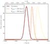 |
Fig. 1 Two different spectral shapes: a single Gaussian (solid), and a P-Cygni profile (dashed). |
We found that the input spectral shape only weakly affects the surface brightness (SB) or the polarization of the LAB. With the P-Cygni-like profiles, the degree of polarization tends to be slightly higher by a few percents because much of the scattering gas is infalling. Hence, by using the Gaussian profile as our fiducial model for the Lyα spectrum at the boundary of the ISM, we expect to derive a lower limit of the estimated contribution of the galactic emission.
2.3.3. Sampling the extragalactic gas emission
In the blob simulation of RB12, the ionisation state of the gas, its temperature, and the density are directly given by Ramses-RT, and the local emissivity of the gas is computed as ε = εcoll + εrec. In this specific simulation, the extragalactic gas contributes to the total Lyα luminosity by Lgas ≃ 2.11 × 1043 erg s-1. Thirty-six percent of the luminosity of the extragalactic gas comes from the CGM, and more than 55% come from the streams. As the luminosity of the gas varies by more than 12 orders of magnitude among ~ 4 × 10⁶ AMR cells, we cannot afford to sample the gas luminosity by sending a number of photons proportional to the cell luminosity from each cell. By sending at least 100 photons per cell, such a proportional sampling would require the prohibitive total of 1017 photons. We chose instead to send a fixed number of 150 photons from each of the ~ 256 500 most luminous cells of the simulation. This restricts the range of luminosities to only three orders of magnitude. The average luminosity of the 100 faintest cells in our sample is approximately 2300 times lower than that of the average luminosity of the 100 brightest cells. Doing so, each photon will carry  of its mother cell luminosity. We evaluated the impact of our (under-) sampling strategy of the simulation cells using a bootstrap method (see Appendix B for details).
We fixed the limit of 256 500 cells after ensuring that taking more gas into account would not noticeably affect our results. This (limited) set of cells still accounts for ~ 97% of the total blob luminosity (Lgas = 2.04 × 1043 erg s-1). Table 1 compares the luminosity budget for the whole halo and for the sampled cells. As expected, the 256 500 brightest cells that we cast photons from capture most of the luminosity of the CGM (99.9%) and of the cold streams (97.4%) but leaves out about a third of the luminosity of the very diffuse gas. We miss a very small fraction (~1%) of the total luminosity of the very diffuse gas; this does not affect our results.
Luminosity budget in 1042 erg s-1.
The last physical parameter to determine before casting a Lyα photon is its exact wavelength. We drew the initial frequency of each Monte Carlo photon from a Gaussian distribution, centred on νLyα in the frame of the emitting cell. We set the width of this Gaussian line to be  , where vth is the typical velocity of atoms due to thermal motions, and vturb = 10 km s-1 describes the sub-grid turbulence.
In Fig. 3 we illustrate the source distribution for the extragalactic emission.
2.4. Mock observations
To observe our simulated LAB, we collected the photons when they passed the virial radius. Photons exiting the halo were selected in a cone of 15° around the projection direction. We discuss the effect of the selection on the results in Appendix C. We then projected these photons on a grid of 200 pixels on a side (equivalent to 0.125′′). We now describe how we built polarization maps from MCLya output.
We assumed that each Monte Carlo photon is equivalent to a (polarized) beam of light and that two independent photons are incoherent. This means that each pixel of our mock maps receives a mixture of independent linearly polarized beams. The Stokes parameters are thus given by Chandrasekhar (1960, Eq. (164)), 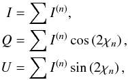 (4)where I(n) defines the intensity of each beam and χn is the polarization angle of each beam (with respect to a set of axes). Here, we have no V Stokes parameter since we assumed a purely linear polarization for each Monte Carlo photon.
With Eq. (4) we built the I, Q, and U maps in a set of chosen directions from the output of MCLya and smoothed them with a Gaussian of full width at half-maximum 1′′ to mimic a typical point spread function (PSF) in observations.
We extracted the degree of polarization  and the angle of polarization χ in each pixel with
  (5)and
  (6)We computed the degree and angle of polarization in pixels with more than five MC photons after smoothing. This tends to overestimate the degree of polarization at high radius, but has no effect in the inner 40 kpc.
3. Results
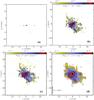 |
Fig. 2 a) Positions of the young massive stars from which we cast Lyα photons that make up the galactic contribution. b) SB map of the extragalactic emission region. c) SB map of the blob after transfer, with both galactic and extragalactic contribution to Lyα emission. d) Mock observation of the halo with a seeing of 1″. The dashes show polarization, and the contours mark 1.4 × 10⁻¹⁸ erg s-1 cm-2 arcsec-2 and 10-19 erg s-1 cm-2 arcsec-2. |
In Fig. 3 we show a mock image of our simulated blob. The inner iso-contours mark surface brightnesses of 1.4 × 10⁻¹⁸ erg s-1 cm-2 arcsec-2, which are typical of current observational limits. The outer contours at 10-19 erg s-1 cm-2 arcsec-2 show what we might see in deep VLT/MUSE observations. The bars show the polarization direction and amplitude (with a scaling indicated in the bottom left corner of the plot) in different points chosen for illustration purposes1.
We now analyse our results and compare them to observations. We followed these steps: first, we produced mock observations along multiple lines of sight (LOS). Then, we computed SB profiles and polarization profiles for each LOS. Finally, we averaged the profiles over all LOS.
3.1. Surface brightness profiles
RB12 argued that adding Lyα scattering effects to their simulation would not change the observed area of the blob by much. They also neglected the (galactic) contribution of star formation to the total Lyα luminosity. With our simulation, we can compare the effect of scattering to that of a typical PSF on the observed SB profile for the extragalactic contribution to the luminosity of the LAB. In Fig. 3 we show the SB profile before and after transfer (in blue and red, respectively), and before and after the convolution with a PSF (dashed and solid line, respectively). We find that Lyα scattering leads to a redistribution of light out to larger radii than a Gaussian PSF of 1 arcsec. This strongly affects the inner (r< 5 kpc) and outer (r> 25 kpc) profile, as shown by the difference between the blue and red dashed curves. Coincidentally, however, at the level of 1.4 × 10⁻¹⁸ erg s-1 cm-2 arcsec-2, the effect of scattering is similar to that of the PSF. At this surface brightness, we find that neglecting radiative transfer leads to an underestimate of the LAB radius of only ΔR/R ≃ 8%, that is, a relative error on the blob area of ΔA/A ≃ 16%.
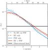 |
Fig. 3 Effect of scattering compared to that of a PSF on the observed SB profile for the extragalactic contribution to the luminosity. The SB profiles before (after) transfer are shown in blue (red), the profiles with (without) PSF are represented as a solid (dashed) line. Note that only the emission from extra-galactic gas is taken into account here. |
The observed surface brightness profiles provide a strong constraint on the properties of the HzLANs. In Fig. 4 we compare the total surface brightness profile of our simulated blob (taking both galactic and extragalactic Lyα emission into account, as discussed in Sect. 2.3) and a set of observational contraints. The thin orange lines show the profiles of our simulated blob along each of the 100 lines of sight, and the thick red solid (resp. dashed) line shows the median profile (first and third quartiles). We also plot the galactic (lower dotted line) and extragalactic contributions (upper dotted line) to the luminosity. The galactic component dominates at the centre (< 1″) and is soon overtaken by extragalactic emission, which represents about 90% of the signal at all radii > 2 arcsec. The blue dashed line shows the average profile of 11 LABs observed at z = 2−3 (Steidel et al. 2011), and the blue dotted line is the fit given by Prescott et al. (2012) for LABd05, rescaled to z = 3 (however, LABd05 is five times brighter than our blob). We compare the results to the average surface brightness profile of a sample of 130 Lyα emitters (LAE) in regions with a high LAE overdensity (blue circles) taken from Matsuda et al. (2012). The teal squares show H11 observation of LAB1 (Steidel et al. 2000), rescaled so that its total luminosity is similar to H2.
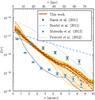 |
Fig. 4 Comparison of SB profiles. The red solid line is the SB profile expected from the sum of both gas and galactic contributions; the red dashed lines show the first and third quartiles. The thin orange lines represents the profile for each LOS. The upper (lower) black dotted line shows the the extra-galactic (galactic) contributions. Two observational data taken from the literature (see text box) are shown in blue, data points are H11 observations (teal) and the Matsuda et al. (2012) stacked profile (blue). |
Figure 4 shows that our profile agrees with that of Prescott et al. (2012), especially when we focus on the extragalactic contribution (upper black dotted curve). We point out that this was already true for the profile without scattering found by RB12 (see their Fig. 13). The LAE used in the sample of Matsuda et al. (2012) are significantly smaller and fainter than our LAB, but they are remarkably similar to the galactic Lyα emission of our simulation. Our result seems to be inconsistent with the profile from Steidel et al. (2011). However, a good agreement was not expected: RB12 argued that only their most massive halo H3 fit the results from Steidel et al. (2011). Maybe more importantly since it is the only positive polarimetric observation, our results are in correct agreement with H11 data, although they are slightly steeper at large radii.
3.2. Polarization
For each plot in this section (Figs. 5 and 6), the 100 LOS are depicted as thin orange lines. The red solid line represents the median profile. The interval between the two dashed red lines contains 50% of the LOS. With the bootstrap method described in Appendix B, we estimate the error due to our cell sampling strategy and show it as a red area around the median profile.
3.2.1. Polarization profile
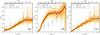 |
Fig. 5 Polarization radial profiles for a) extragalactic emission; b) galactic emission; and c) the overall Lyα emission. The thin orange lines show the profile corresponding to each LOS; the solid red line is the median profile; the dispersion along different LOS is represented by the two dashed red lines (first and third quartiles). The red area shows the 3σ confidence limits inferred from our bootstrap experiment (see Appendix B). The data points are taken from H11. |
To compare our simulation to H11 polarimetric observations, we need to characterise both the direction and the degree of polarization. To describe the latter, we computed radial profiles for the different components of the Lyα emission. Figure 5 displays the polarization profiles obtained for each component of the signal: emission from extragalactic gas (panel a), Lyα photons produced in the star-forming ISM (panel b), and the combination of the two (panel c). We compare these results with H11 observations, displayed as filled squares with error bars.
The main result of our study is that the polarization profile produced only by the extragalactic gas rise up to 15%, similar to what is observed by H11. This is unexpected: in this non-idealised setup, the extended emission does not cancel out the polarization. This is mainly because the gas distribution is not homogeneous. Even if we refer to the extragalactic emission as an extended source, it is still much more concentrated in the inner region of the blob, as can be seen in the SB profiles of Fig. 4. Dijkstra & Loeb (2009) suggested that the low volume filling factor of the cold streams would prevent the polarization from arising: there is indeed only little chance that a photon that has escaped from a filament will encounter another one before it is observed. However, we found that the photons responsible for the polarization signal mostly travel radially outwards inside the gas, and then escape their filament at the last scattering (see Sect. 3.2.3).
Furthermore, if we consider the galactic component alone, it is clearly inconsistent with H11 observations: the polarization profile is too steep in the central region, meaning that it is compulsory to take the extended emission into account. We checked that this is not an artefact resulting from the choice of the pixelization. While the profiles presented in Fig. 5 correspond to maps with a pixelization (≳0.12″) much finer than the spatial resolution of the observations, we verified that our results hold for a coarser spatial resolution (~ 1.25″). In the experiment with larger pixels, we noted a decrease of the degree of polarization at large distance (≳ 5″), but not strong enough to alter our results.
3.2.2. Polarization angle
The second observed attribute we can produce is the polarization angle. Qualitatively, the direction of polarization in a given pixel of the map seems to be aligned in circles around the centre of the blob, as shown in Fig. 3. A more quantitative study can confirm this: for each pixel on the map, we computed the difference between the polarization angle and the tangential angle. We then rebinned the resulting distribution to match H11 bins, and the result is shown in Fig. 6. The polarization angle is not random at all, but rather aligned with the tangential angle.
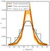 |
Fig. 6 Distribution of the angle between polarization and tangential direction. The thin orange lines show the profile corresponding to each LOS; the solid red line is the median profile, and the two dashed red lines denote the first and third quartiles. The red area shows the 3σ confidence limits inferred from our bootstrap experiment (see Appendix B), and the teal line is the distribution taken from H11. We show the profile we obtain by assuming some noise in the angle measurement in black. |
This is qualitatively compatible with the results of H11: they also found a clustering of the values around zero. A more quantitative comparison shows that our distribution is much more peaked around zero. However, we have no measurement error on the polarization angle in each pixel in our numerical experiment, which is not true in the case of observations. We assumed a Gaussian error of width 20° on the angle measurement and recomputed the angle distribution. The result, shown as the black curve in Fig. 6, agrees much better with the observations.
3.2.3. Origin of the polarization
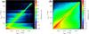 |
Fig. 7 Distribution of the radii of emission, rem, for each observation radius, robs, weighted by the (normalised) luminosity of the photons. These radii are not distances to the halo centre, but projected onto the observation plane perpendicular to the line of sight for each simulated photon. a) Galactic component; b) extragalactic component. |
Polarization is a geometrical effect that arises naturally in a configuration with centrally concentrated emission that is scattered outwards. From our numerical experiment, we find that extended extragalactic Lyα emission generates a polarized nebula with a relatively strong polarization signal (15% close to the virial radius). This polarization emerges for the same reason: photons statistically scatter outwards before they are observed.
In Fig. 7 we show the 2D histogram (weighted by luminosity) of the projected emission radius rem (where the MC photons are cast) as a function of the projected observed radius robs (where the MC photons last scatter before they are observed). These projected radii are projections onto the plane perpendicular to the direction of propagation of each MC photon. The left (resp. right) panel shows the distribution of projected rem versus projected robs for the galactic (resp. extragalactic) emission. The prominent feature in both cases is the diagonal line, showing that a significant part of observed photons escape close to their emission site even for galactic emission. The asymmetry between the upper and lower half planes illustrates that more photons escaping at a given robs were emitted at a smaller radius. There is a strong (expected) asymmetry for the galactic emission, and a lighter but noticeable asymmetry in the extragalactic case. This explains the steeper polarization profile for the galactic sources than for the extragalactic sources (see Fig. 5). Each horizontal feature in the left panel corresponds to the location of a Lyα source (satellite galaxy) and illustrates the fact that a significant fraction of photons emitted by external sources (with large rem) also scatter in the central parts of the blob and escape at smaller robs. To summarize, for a significant fraction of the Lyα MC photons (more than 55% of the extragalactic luminosity), the emission location is close to the last scattering place. These Lyα photons do not contribute to the observed polarization.
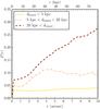 |
Fig. 8 Polarization profile obtained by selecting photons according to the distance between the emission and the last scattering. |
To sketch this out in a more quantitative manner, we now focus on the extragalactic component (i.e. cooling radiation from the gas). In Fig. 8 we show the polarization signal that is due to extragalactic MC photons that have travelled less than 5 kpc (resp. between 5 and 20 kpc, and more than 20 kpc) as the yellow (resp. dot-dashed orange and dashed red) curve. The photons that travel more are responsible for the polarization. We note that by selection, they tend to come from the central regions as well.
3.3. Scattering in the IGM
So far, we limited our analysis to the photons scattered within the virial radius of the halo, thus assuming that the effect of the IGM was negligible. Previous works by DL08, for example, showed that for a galaxy without strong outflows (as it is the case in our simulation), radiation scattered in the IGM carries a low polarization level, however. This is typically around 2% and has a very flat surface brightness profile. While they travel through the IGM, Lyα photons become blueshifted and might experience a significant number of scatterings, which would reduce the level of polarization.
While we cannot fully describe the Lyα resonant scattering in the IGM with the current version of MCLya (a volume larger than currently investigated would not fit in the computer memory), we can still estimate to which extent our results would be affected by taking additional scattering into account. We denote by f the fraction of the luminosity that will scatter in the IGM. To compute the value of f, we assume that photons escaping the halo redwards of the lya line will be observed directly and that a fraction of  of the blue photons will undergo further scattering, with
  being the mean IGM transmission at z ~ 3 (see e.g. Faucher-Giguère et al. 2008; Inoue et al. 2014). We can compute the value of f from the spectrum averaged over all directions: a fraction fb ~ 60.5% of the photons are bluewards of λLyα, resulting in
  , meaning that on average, approximately 20% of the photons in our simulation are scattered in the IGM. While this is only a first-order approximation, it gives a reasonable estimate of the amount of photons that are scattered in the IGM. We discuss its validity in Appendix D. Following the findings of DL08 that scattering in the IGM results in a rather flat profile, and to maximise the effect, we uniformly redistributed the total luminosity contributed by these photons in a patch of sky of 10 Rvir on a side, such that the photons have travelled ~ up to 5 Rvir, corresponding to an area larger than the maps of Fig. 2 by a factor of 25. We assigned to these photons a degree of polarization of 2%, following the results of DL08 and assumed that the linear polarization follows the same pattern around the galaxy as before. More precisely, we computed the IIGM, QIGM, and UIGM maps as
 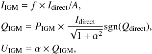 (7)where A = 25 is the dilution factor due to the larger area over which photons are redistributed, PIGM = 0.02 is the polarization level of the radiation scattered in the IGM, and
  . We then summed the direct and scattered contributions as
 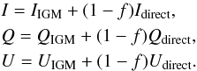 (8)We present the results of this experiment in Fig. 9. The red lines are the same as in Fig. 5. The dash-dotted black line shows the polarization profile we obtain with the above calculation, assuming that all the photons scattered by the IGM beyond Rvir are seen as coming from within a extended surface of side 10 Rvir. We find that quantitatively, the effect is small, and that the signal remains within the error bars of Fig. 5. More importantly, the deviation occurs are large radii, and the IGM has no effect on the signal within ~ 40 kpc where the constraints are stronger. We note that this is likely to overestimate the effect on the IGM on the polarization profile. Based on the work of Laursen et al. (2011), we estimated that about 5% of the photons crossing Rvir are scattered within 5 Rvir (compared to 20% scattered in total, see Appendix D). This means that most photons scatter very far away from the source. This implies that the luminosity contributed by those photons is diluted across a much larger area. In Fig. 9 the orange dotted curve shows the more realistic polarization profile that we obtain when we only redistribute these 5% of the luminosity within an area of 10 Rvir on a side. It is barely distinguishable from the model without IGM (see Appendix D). Keeping in mind that our model is only a first-order approximation, it seems that scattering of Lyα radiation well outside the virial radius is not likely to alter our polarization profiles dramatically. Strictly speaking, however, all the previous results on the polarization should be regarded as upper limits.
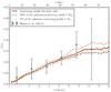 |
Fig. 9 Effect of the IGM on the polarization profile. Compared to the profile right outside of the halo (solid red line), scattering in the IGM (dash-dotted and dotted black lines) reduces slightly the degree of polarization at large radii, but not much (if we redistribute the photons in a large enough area). |
4. Discussion and conclusions
We have performed Lyα radiative transfer through a LAB simulation, as previously discussed by RB12. We considered the galactic and extragalactic contributions to the Lyα luminosity separately and followed the polarization of Lyα photons during their journey through the blob.
Our main results are the following:
-
We confirm that the results of DL08 for their idealised coolingmodel hold for a more complex but realistic distribution of gas: thecooling radiation produces a polarized signal. Furthermore, thepolarization radial profiles computed by only taking theextragalactic contribution into account is compatible withobservational data.
-
A Lyα escape fraction of the galactic contribution of 5% is enough to find a good agreement with H11 results. This means that a non-negligible extragalactic contribution to the luminosity is compatible with current polarimetric observations.
-
The (galactic) contribution of the star formation to the Lyα luminosity of a HzLAN with no associated AGN is small, and the effect of the scattering on the SB profile is similar to the effect of a convolution with a PSF. This confirms that the extent of the HzLANs presented in RB12 is correct.
It is important to stress some of the potential limits of our investigation. First, the galactic contribution is uncertain in our simulation because the structure of the ISM is under-resolved. Nevertheless, our estimation of the star formation rate (SFR ≃ 160 M⊙ yr-1, shared between all the galaxies in the halo) is typical of giant LABs (Fardal et al. 2001). The total galactic contribution to the Lyα luminosity is the product of the intrinsic galactic luminosity by the Lyα escape fraction fesc, however. Our results are consistent with H11 data with a typical value of fesc = 5% (Garel et al. 2012). In our model, the spectral shape of the stellar component of the Lyα emission can be arbitrarily selected. However, we have tested that the input spectrum of the stellar component has little effect on the SB and polarization profiles, provided the choice of the spectrum is physical enough (Gaussian profile, P-Cygni-like profile). More work is needed to produce strong predictions for spectro-polarimetric studies. We also assumed that the Lyα photons are isotropically emitted from the galaxies. From Verhamme et al. (2012), we know that this is not true. However, since (i) we have several galaxies in the halo and (ii) the photons scatter strongly in the CGM, there should be no favoured escape direction. This is corroborated by the low polarization degree in the inner regions of the blob. Another possible problem is that the simulation we used is somewhat idealised: the RB12 halo includes neither cooling below 104 K nor supernova feedback. Adding these ingredients might alter the structure of the central region blob (CGM and inner parts of the streams), and this is precisely where most of the extragalactic gas contribution to Lyα emission comes from. More work is needed to carefully quantify the effect of cooling and feedback on our results. Finally, we must note that we only took scattering within the virial radius into account, which led to a most likely small overestimation of the degree of polarization we computed at large radius. Lastly, we must be aware of the lack of statistics on HzLANs polarimetric studies. There are currently only two positive observations of polarization around a giant HzLANs (Hayes et al. 2011; Humphrey et al. 2013), and we have no certainty that our blob is a perfectly typical giant blob. However, the stability of the polarization and SB profiles when changing the LOS is reassuring. Once again, further work is needed to address this question.
We here only considered two possible sources for the Lyα radiation: cooling radiation emitted by the accretion-heated gas, and Lyα emission from the H ii star-forming regions. We did not investigate the possibility that the gas is ionised by central AGN. Overzier et al. (2013) suggested that virtually all the most luminous HzLANs are associated with AGNs and that the for the less luminous HzLANs, the central black-hole is just not in an active state. This is compatible with the scenario of Reuland et al. (2003). In this picture, HzLANs are the signatures of the first stage of the building of massive galaxies. As the gas falls onto the halo, it dissipates its energy through Lyα cooling, producing a blob. As the gas accretes, stars and galaxies begin to form and merge, which at some point triggers the central AGN.
The Lyα polarization radial profile arising from a non-idealised distribution of gas appears finally as a rich and complex tool. This work is a first step towards a better understanding of Lyα polarimetric observations. However, another step needs to be made to use them to study the relative contributions of extragalactic versus star-formation channels of Lyα production.
We only show the polarization signal in pixels that have more than ten Monte Carlo photons.
Acknowledgments
The authors would like to thank Matthew Hayes and Claudia Scarlata for stimulating discussions, and the anonymous referee for insightful comments. We wish to thank Gérard Massacrier and Stéphanie Courty for valuable help at the early stages of the project. We are also grateful to Léo Michel-Dansac, whose help with the computing centres was priceless. J.R. acknowledges financial support from the Marie Curie Initial Training Network ELIXIR of the European Commission under contract PITN-GA-2008-214227, the European Research Council under the European Union’s Seventh Framework Programme (FP7/2007−2013)/ERC Grant agreement 278594-GasAroundGalaxies, and the Marie Curie Training Network CosmoComp (PITN-GA-2009-238356). The initial simulations of the blob were performed using the HPC resources of CINES under the allocation c2012046642 made by GENCI (Grand Equipement National de Calcul Intensif), and all the other ones were performed using the computing resources at the CC-IN2P3 Computing Centre (Lyon/Villeurbanne – France), a partnership between CNRS/IN2P3 and CEA/DSM/Irfu.
References
- Basu-Zych, A., & Scharf, C. 2004, ApJ, 615, L85 [NASA ADS] [CrossRef] [Google Scholar]
- Birnboim, Y., & Dekel, A. 2003, MNRAS, 345, 349 [NASA ADS] [CrossRef] [Google Scholar]
- Brooks, A. M., Governato, F., Quinn, T., Brook, C. B., & Wadsley, J. 2009, ApJ, 694, 396 [NASA ADS] [CrossRef] [Google Scholar]
- Bunker, A., Smith, J., Spinrad, H., Stern, D., & Warren, S. 2003, Ap&SS, 284, 357 [NASA ADS] [CrossRef] [Google Scholar]
- Callaway, J., Unnikrishnan, K., & Oza, D. H. 1987, Phys. Rev. A, 36, 2576 [NASA ADS] [CrossRef] [Google Scholar]
- Cantalupo, S., Porciani, C., Lilly, S. J., & Miniati, F. 2005, ApJ, 628, 61 [NASA ADS] [CrossRef] [Google Scholar]
- Cantalupo, S., Arrigoni-Battaia, F., Prochaska, J. X., Hennawi, J. F., & Madau, P. 2014, Nature, 506, 63 [NASA ADS] [CrossRef] [Google Scholar]
- Chambers, K. C., Miley, G. K., & van Breugel, W. J. M. 1990, ApJ, 363, 21 [NASA ADS] [CrossRef] [Google Scholar]
- Chandrasekhar, S. 1960, Radiative transfer (New York: Dover) [Google Scholar]
- Chapman, S. C., Lewis, G. F., Scott, D., et al. 2001, ApJ, 548, L17 [NASA ADS] [CrossRef] [Google Scholar]
- Christensen, L., Jahnke, K., Wisotzki, L., & Sánchez, S. F. 2006, A&A, 459, 717 [NASA ADS] [CrossRef] [EDP Sciences] [Google Scholar]
- Code, A. D., & Whitney, B. A. 1995, ApJ, 441, 400 [NASA ADS] [CrossRef] [Google Scholar]
- Dekel, A., & Birnboim, Y. 2006, MNRAS, 368, 2 [NASA ADS] [CrossRef] [Google Scholar]
- Dey, A., Bian, C., Soifer, B. T., et al. 2005, ApJ, 629, 654 [NASA ADS] [CrossRef] [Google Scholar]
- Dijkstra, M., & Loeb, A. 2008, MNRAS, 386, 492 [NASA ADS] [CrossRef] [Google Scholar]
- Dijkstra, M., & Loeb, A. 2009, MNRAS, 400, 1109 [NASA ADS] [CrossRef] [Google Scholar]
- Dijkstra, M., Haiman, Z., & Spaans, M. 2006, ApJ, 649, 14 [NASA ADS] [CrossRef] [Google Scholar]
- Erb, D. K., Bogosavljević, M., & Steidel, C. C. 2011, ApJ, 740, L31 [NASA ADS] [CrossRef] [Google Scholar]
- Fardal, M. A., Katz, N., Gardner, J. P., et al. 2001, ApJ, 562, 605 [NASA ADS] [CrossRef] [Google Scholar]
- Faucher-Giguère, C.-A., Lidz, A., Hernquist, L., & Zaldarriaga, M. 2008, ApJ, 688, 85 [NASA ADS] [CrossRef] [Google Scholar]
- Faucher-Giguère, C.-A., Kereš, D., Dijkstra, M., Hernquist, L., & Zaldarriaga, M. 2010, ApJ, 725, 633 [NASA ADS] [CrossRef] [Google Scholar]
- Francis, P. J., Woodgate, B. E., Warren, S. J., et al. 1996, ApJ, 457, 490 [NASA ADS] [CrossRef] [Google Scholar]
- Furlanetto, S. R., Schaye, J., Springel, V., & Hernquist, L. 2005, ApJ, 622, 7 [NASA ADS] [CrossRef] [Google Scholar]
- Fynbo, J. U., Møller, P., & Warren, S. J. 1999, MNRAS, 305, 849 [NASA ADS] [CrossRef] [Google Scholar]
- Garel, T., Blaizot, J., Guiderdoni, B., et al. 2012, MNRAS, 422, 310 [NASA ADS] [CrossRef] [Google Scholar]
- Geach, J. E., Matsuda, Y., Smail, I., et al. 2005, MNRAS, 363, 1398 [NASA ADS] [CrossRef] [Google Scholar]
- Geach, J. E., Smail, I., Chapman, S. C., et al. 2007, ApJ, 655, L9 [NASA ADS] [CrossRef] [Google Scholar]
- Geach, J. E., Bower, R. G., Alexander, D. M., et al. 2014, ApJ, 793, 22 [NASA ADS] [CrossRef] [Google Scholar]
- Goerdt, T., Dekel, A., Sternberg, A., et al. 2010, MNRAS, 407, 613 [Google Scholar]
- Gould, A., & Weinberg, D. H. 1996, ApJ, 468, 462 [NASA ADS] [CrossRef] [Google Scholar]
- Haiman, Z., & Rees, M. J. 2001, ApJ, 556, 87 [NASA ADS] [CrossRef] [Google Scholar]
- Haiman, Z., Spaans, M., & Quataert, E. 2000, ApJ, 537, L5 [NASA ADS] [CrossRef] [Google Scholar]
- Hamilton, D. R. 1947, ApJ, 106, 457 [NASA ADS] [CrossRef] [Google Scholar]
- Hayes, M., Scarlata, C., & Siana, B. 2011, Nature, 476, 304 [NASA ADS] [CrossRef] [Google Scholar]
- Heckman, T. M., Lehnert, M. D., Miley, G. K., & van Breugel, W. 1991, ApJ, 381, 373 [NASA ADS] [CrossRef] [Google Scholar]
- Hui, L., & Gnedin, N. Y. 1997, MNRAS, 292, 27 [Google Scholar]
- Humphrey, A., Vernet, J., Villar-Martín, M., et al. 2013, ApJ, 768, L3 [NASA ADS] [CrossRef] [Google Scholar]
- Inoue, A. K., Shimizu, I., Iwata, I., & Tanaka, M. 2014, MNRAS, 442, 1805 [NASA ADS] [CrossRef] [Google Scholar]
- Keel, W. C., Cohen, S. H., Windhorst, R. A., & Waddington, I. 1999, AJ, 118, 2547 [NASA ADS] [CrossRef] [Google Scholar]
- Kennicutt, Jr., R. C. 1998, ApJ, 498, 541 [NASA ADS] [CrossRef] [Google Scholar]
- Kereš, D., Katz, N., Weinberg, D. H., & Davé, R. 2005, MNRAS, 363, 2 [NASA ADS] [CrossRef] [Google Scholar]
- Kereš, D., Katz, N., Fardal, M., Davé, R., & Weinberg, D. H. 2009, MNRAS, 395, 160 [NASA ADS] [CrossRef] [Google Scholar]
- Kollmeier, J. A., Zheng, Z., Davé, R., et al. 2010, ApJ, 708, 1048 [NASA ADS] [CrossRef] [Google Scholar]
- Laursen, P., Sommer-Larsen, J., & Razoumov, A. O. 2011, ApJ, 728, 52 [NASA ADS] [CrossRef] [Google Scholar]
- Lee, H.-W., & Ahn, S.-H. 1998, ApJ, 504, L61 [NASA ADS] [CrossRef] [Google Scholar]
- Matsuda, Y., Yamada, T., Hayashino, T., et al. 2004, AJ, 128, 569 [NASA ADS] [CrossRef] [Google Scholar]
- Matsuda, Y., Yamada, T., Hayashino, T., Yamauchi, R., & Nakamura, Y. 2006, ApJ, 640, L123 [NASA ADS] [CrossRef] [Google Scholar]
- Matsuda, Y., Iono, D., Ohta, K., et al. 2007, ApJ, 667, 667 [NASA ADS] [CrossRef] [Google Scholar]
- Matsuda, Y., Yamada, T., Hayashino, T., et al. 2012, MNRAS, 425, 878 [NASA ADS] [CrossRef] [Google Scholar]
- Mori, M., Umemura, M., & Ferrara, A. 2004, ApJ, 613, L97 [NASA ADS] [CrossRef] [Google Scholar]
- Nilsson, K. K., Fynbo, J. P. U., Møller, P., Sommer-Larsen, J., & Ledoux, C. 2006, A&A, 452, L23 [NASA ADS] [CrossRef] [EDP Sciences] [Google Scholar]
- Ocvirk, P., Pichon, C., & Teyssier, R. 2008, MNRAS, 390, 1326 [NASA ADS] [Google Scholar]
- Ohyama, Y., Taniguchi, Y., Kawabata, K. S., et al. 2003, ApJ, 591, L9 [NASA ADS] [CrossRef] [Google Scholar]
- Osterbrock, D. E., & Ferland, G. J. 2006, Astrophysics of gaseous nebulae and active galactic nuclei (Sausalito, CA: University Science Books) [Google Scholar]
- Ouchi, M., Ono, Y., Egami, E., et al. 2009, ApJ, 696, 1164 [NASA ADS] [CrossRef] [Google Scholar]
- Overzier, R. A., Nesvadba, N. P. H., Dijkstra, M., et al. 2013, ApJ, 771, 89 [NASA ADS] [CrossRef] [Google Scholar]
- Palunas, P., Teplitz, H. I., Francis, P. J., Williger, G. M., & Woodgate, B. E. 2004, ApJ, 602, 545 [NASA ADS] [CrossRef] [Google Scholar]
- Prescott, M. K. M., Kashikawa, N., Dey, A., & Matsuda, Y. 2008, ApJ, 678, L77 [NASA ADS] [CrossRef] [Google Scholar]
- Prescott, M. K. M., Smith, P. S., Schmidt, G. D., & Dey, A. 2011, ApJ, 730, L25 [NASA ADS] [CrossRef] [Google Scholar]
- Prescott, M. K. M., Dey, A., Brodwin, M., et al. 2012, ApJ, 752, 86 [NASA ADS] [CrossRef] [Google Scholar]
- Prescott, M. K. M., Dey, A., & Jannuzi, B. T. 2013, ApJ, 762, 38 [NASA ADS] [CrossRef] [Google Scholar]
- Reuland, M., van Breugel, W., Röttgering, H., et al. 2003, ApJ, 592, 755 [NASA ADS] [CrossRef] [Google Scholar]
- Rosdahl, J., & Blaizot, J. 2012, MNRAS, 423, 344 [NASA ADS] [CrossRef] [Google Scholar]
- Rosdahl, J., Blaizot, J., Aubert, D., Stranex, T., & Teyssier, R. 2013, MNRAS, 436, 2188 [NASA ADS] [CrossRef] [Google Scholar]
- Rybicki, G. B., & Loeb, A. 1999, ApJ, 520, L79 [NASA ADS] [CrossRef] [Google Scholar]
- Saito, T., Shimasaku, K., Okamura, S., et al. 2006, ApJ, 648, 54 [NASA ADS] [CrossRef] [Google Scholar]
- Saito, T., Matsuda, Y., Lacey, C. G., et al. 2015, MNRAS, 447, 3069 [NASA ADS] [CrossRef] [Google Scholar]
- Scarlata, C., Colbert, J., Teplitz, H. I., et al. 2009, ApJ, 706, 1241 [NASA ADS] [CrossRef] [Google Scholar]
- Smith, D. J. B., Jarvis, M. J., Simpson, C., & Martínez-Sansigre, A. 2009, MNRAS, 393, 309 [NASA ADS] [CrossRef] [Google Scholar]
- Steidel, C. C., Adelberger, K. L., Shapley, A. E., et al. 2000, ApJ, 532, 170 [Google Scholar]
- Steidel, C. C., Bogosavljević, M., Shapley, A. E., et al. 2011, ApJ, 736, 160 [NASA ADS] [CrossRef] [Google Scholar]
- Stenflo, J. O. 1980, A&A, 84, 68 [NASA ADS] [Google Scholar]
- Taniguchi, Y., & Shioya, Y. 2000, ApJ, 532, L13 [NASA ADS] [CrossRef] [Google Scholar]
- Teyssier, R. 2002, A&A, 385, 337 [NASA ADS] [CrossRef] [EDP Sciences] [Google Scholar]
- van de Voort, F., & Schaye, J. 2012, MNRAS, 423, 2991 [NASA ADS] [CrossRef] [Google Scholar]
- van de Voort, F., Schaye, J., Booth, C. M., Haas, M. R., & Dalla Vecchia, C. 2011, MNRAS, 414, 2458 [NASA ADS] [CrossRef] [Google Scholar]
- van Ojik, R., Roettgering, H. J. A., Miley, G. K., & Hunstead, R. W. 1997, A&A, 317, 358 [NASA ADS] [Google Scholar]
- Verhamme, A., Schaerer, D., & Maselli, A. 2006, A&A, 460, 397 [NASA ADS] [CrossRef] [EDP Sciences] [Google Scholar]
- Verhamme, A., Dubois, Y., Blaizot, J., et al. 2012, A&A, 546, A111 [NASA ADS] [CrossRef] [EDP Sciences] [Google Scholar]
- Villar-Martín, M., Vernet, J., di Serego Alighieri, S., et al. 2002, MNRAS, 336, 436 [NASA ADS] [CrossRef] [Google Scholar]
- Villar-Martín, M., Sánchez, S. F., Humphrey, A., et al. 2007, MNRAS, 378, 416 [NASA ADS] [CrossRef] [Google Scholar]
- Weidinger, M., Møller, P., & Fynbo, J. P. U. 2004, Nature, 430, 999 [NASA ADS] [CrossRef] [PubMed] [Google Scholar]
- Whitney, B. A. 2011, Bull. Astron. Soc. India, 39, 101 [NASA ADS] [Google Scholar]
- Yang, Y., Zabludoff, A., Tremonti, C., Eisenstein, D., & Davé, R. 2009, ApJ, 693, 1579 [NASA ADS] [CrossRef] [Google Scholar]
- Yang, Y., Zabludoff, A., Eisenstein, D., & Davé, R. 2010, ApJ, 719, 1654 [NASA ADS] [CrossRef] [Google Scholar]
Appendix A: Test of the code
To test the validity of our polarized Lyα transfer code, we compared it to the first case considered by DL08, Lyα scattering on galactic superwinds. This is pictured with a simple toy model: a thin spherical shell of column density NH i = 1019 cm-2 or 1020 cm-2 illuminated by a central source. The radius of the shell is 10 kpc, and the expansion velocity is 200 km s-1. We used a Gaussian profile with a width corresponding to a temperature of T = 104 K for the input spectrum of the Lyα emission.
In their code, DL08 model gas by concentric shells of given densities and velocities, whereas our code uses an AMR grid to describe the gas. To create the shell, we fill an unrefined grid with 5123 cells using Monte Carlo integration with 108 points.
We then cast and follow 106 Monte Carlo photons in this setup to produce a polarization profile using the method described in Sect. 2.4. In Fig. A.1 we compare our results (in red) to the profile of DL08 (black). They agree fairly well both for the NH = 1019 cm-2 shell (solid line) and for the NH = 1020 cm-2 shell (dashed line).
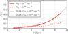 |
Fig. A.1 Polarization profile for an expanding spherical shell. Results from DL08 are shown in black, our results in red. The solid (dashed) line corresponds to a column density of NH = 1019 cm-2 (NH = 1020 cm-2). |
Appendix B: Effect of the sampling
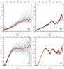 |
Fig. B.1 Polarization profile for different subsets of photons. In all the plots, the red solid line is the median profile; the red dashed lines are the first and third quartiles. The thin grey lines represent the profiles for a) 100 LOS with the same photons subset for the gas emission; b) 100 different photon subsets seen with the same LOS for the gas emission; c) 100 LOS with the same photon subsets for the galactic emission; d) 100 different photon subsets seen with the same LOS for the galactic emission. |
In Sect. 2.3.3 we mentioned that we sampled the Lyα emission from the gas nebula with 150 Monte Carlo photons per simulation cell. With only 150 photons, it is impossible to properly describe all the physics of the Lyα emission in each cell. We need to sample not only the initial position of the photon within the cell (three degrees of freedom), but also the initial propagation direction (three degrees of freedom), the initial frequency (one degree of freedom), and the initial polarization direction (two degrees of freedom). It is impossible to sample this 9D parameter space with only 150 points. The same argument holds for the galactic emission: the initial position is well sampled (the number of photons is much greater than the number of sources), but we still have to sample the six other variables.
To ensure that our results are not just a statistical artefact, we need to assess the robustness of our method and to understand how the (under)sampling might affect our results. For this purpose, we used a bootstrap method, both for the emission from the gas and from the star particles. In the case of the gas emission, we performed the analysis presented in Sect. 3 for each simulation cell with a subset of 120 photons (80%) that were randomly selected. Instead of selecting the random subset per cell, we could have selected 80% of all the photons. However, this experiment would not answer the question of the effect of undersampling each cell. We did this for 100 different randomly selected subsets. For the star particles, we selected random subsets with 80% of all the photons because very many photons are emitted per individual star particle and sampling the initial position of the photon is not a problem. From this, we obtained 100 different profiles (either for polarization or for surface brightness), and the standard deviation σboot of this set of profiles gives an estimate of the error caused by the undersampling of the parameter space. This estimate (as 3σboot) is displayed in our profiles in the main text of the paper as red semi-transparent areas.
The results are displayed in Fig. B.1. The top (bottom) panels show the results of our bootstrap experiment for the extragalactic (galactic) emission. Panels a and c show 100 polarization profiles corresponding to 100 LOS for one of the subsets as thin grey lines (for the extragalactic and galactic emission, respectively). Panels b and d show 100 profiles corresponding to 100 subsets for a given LOS. Following the convention used throughout this paper, the solid red line is the median profile and the two dotted lines show the interquartile range.
It is reassuring to note that the variation over the LOS is much stronger than the variation between photon subsets. This means that our sampling of the Lyα emission has a much weaker effect on the observed polarization profile than does the choice of the LOS.
Appendix C: Selection effects
Because of our limited number of photons, we needed to select photons in a (small) cone around each line of sight. This is an approximation and might change the polarization properties we derive from our analysis. To test this, we performed the same analysis as before, but changed the angular opening of the cone and the minimum number of photons selected to compute the polarization properties in a pixel.
Although we would ideally prefer to estimate the polarization in small beams (~few arcsec), our data do not allow us to measure the polarization signal in beams of less than 3°. Below these scales, the (strong) polarization degree is dominated by noise and its large-scale coherence disappears. We verified this by performing the analysis with an opening angle of 15° and randomly selecting a small fraction of these photons. The fraction corresponds to  . The resulting profile is very similar to the one we obtained by reducing the opening angle to 1°, meaning that the dominant effect here is not the error due to the selection in a cone, but rather the limited number of photons. However, at larger opening angles (from ~ 3 to 60°), we consistently find the same profile as shown in Fig. 5, with small deviations of less than 10%. This suggests that our results, which are robust at 15°, can also be compared to observations made with much smaller beams.
The surface brightness profile is much more robust and is mostly unaffected by these experiments. Even with an 1° cone, the relative error is smaller than 10%.
Appendix D: Scattering in the IGM
In Sect. 3.3 we assumed that  of the photons bluewards of λLyα would be subject to further scattering during their journey through the IGM. In this section, we try to estimate the effect of the IGM on the Lyα photons escaping the halo in more detail.
We used the results of Laursen et al. (2011), who followed the transfer of radiation in the IGM in the vicinity of the Lyα line using a large cosmological simulation. In their Fig. 11, they presented the transmission function of the IGM at various redshifts and for sightlines originating at various distances from the centre of their simulated galaxies. As we fully perform the Lyα RT only up to the virial radius of our blob, we needed to use their transmission function as a proxy for the actual transfer through the IGM. We extracted the curves corresponding to sightlines originating at the virial radius for both z = 2.5 and z = 3.5. We fitted the data using the following ad hoc function T(λ) = T(λ;λ0,Tb,Tmin,σr,σb), which essentially describes an assymetric Gaussian absorption: 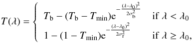 (D.1)where λ0 is the central Lyα wavelength, Tmin is the minimum transmission and Tb corresponds to the transmission far bluewards of Lyα, scaled so that far from the line, the behaviour of T(λ) closely follows the results from Laursen et al. (2011), and σr and σb describe the width of the red and blue parts of the absorption line. We adjusted the parameters to obtain a correct rendering of the results of Laursen et al. (2011) at z = 2.5 and 3.5. We then interpolated each of the parameters to derive the z = 3 curve.
Parameters for T(λ).
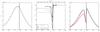 |
Fig. D.1 Left: angle-averaged integrated spectrum of our blob (in black), divided into an extragalactic component (in red) and galactic emission (in blue). Middle: IGM transmission function from Rvir to the observer, fitting the results of Laursen et al. at z = 2.5 (dotted line), z = 3 (solid line) and z = 3.5 (dashed line). Right: resulting spectrum after transmission through the IGM. For all three panels, the vertical line denotes the Lyα wavelength. |
The left panel of Fig. D.1 illustrates the spectrum integrated over all directions of our blob as a black line, with the Lyα wavelength indicated by a vertical line. We computed this spectrum right after the transfer inside the halo, approximately at the virial radius. For the present experiment, we used the Gaussian model discussed in Sect. 2.3.2 for the stellar component (see Fig. 1). The other models yield the same results. The central panel of Fig. D.1 presents the shape of the transmission function T(λ) at z = 3 as a solid black line and the data points extracted from Laursen et al. (2011) as circles (z = 2.5) and crosses (z = 3.5). We give the parameters for our parametrization of T(λ) in Table D.1. Using the method of Laursen et al. (2011), we computed the observed spectrum as the multiplication of our spectrum at Rvir with the IGM transmission function from Rvir to the observer. The result of this is shown as the black line in the right-hand panel of Fig. D.1. We then integrated this to compute the transmitted fraction  and also the fraction of all the photons that are scattered between Rvir and the observer, f. We find
  or f = 13%.
These values are relatively high compared to the canonical value of 0.67 for the transmission of the IGM at z ~ 3. This is because the spectrum resulting from the transfer in our blob is very broad as a result of the large velocity dispersion of the gas. This in turn means that the transmission is dominated by the very blue part of the spectrum. It is noteworthy that the estimate reported by Laursen et al. (2011) of the transmission far from the Lyα line gives much higher values than the observational estimates from Faucher-Giguère et al. (2008), for instance. This overestimate directly translates into an underestimate of f. To try to alleviate this problem and recover both the Lyα forest constraints on the Lyα transmission and the enhanced absorption in the vicinity of galaxies, we used an ad hoc model for the transmission: using the same parametrisation as in Eq. (D.1), we took the transmission blueward of Lyα to be Tb = 0.7. The resulting transmission function is shown in red in the middle panel of Fig. D.1, as is the transmitted spectrum in the right-hand panel. For this model, we find  , or alternatively f = 22%, much closer to the 20% inferred from the naive estimate presented in the text.
Using the results of Laursen et al. (2011), we estimated the fraction of the luminosity transmitted from Rvir to 5 Rvir, which we note T(Rvir,5 Rvir), and approximate as T(Rvir,5 Rvir) ~ T(Rvir,∞) /T(5 Rvir,∞). Here, T(x,∞) is the transmission between radius x and the observer, which we extracted from Laursen et al. (2011) as explained above. We obtain  , meaning that only 5% of the photons are scattered in a shell between Rvir and 5 Rvir. The assumption that 20% of the luminosity is redistributed in a sphere of 5 Rvir will therefore overestimate the effect of the IGM on the polarization profile of our LAB. In the text, we show a model for which only 5% of the photons are redistributed in that sphere of 5 Rvir, but this time, it might very well underestimate the effect of the IGM. Indeed, if most of these photons have their locus of last scattering well inside the 5 Rvir sphere, we should redistribute the luminosity in a much more narrow area. In Fig. D.2 we compare the effect of the scattering inside the IGM on the polarization profile assuming either that 20% of the luminosity is redistributed in a sphere of 5 Rvir (dash-dotted black line) or that 5% of the luminosity is redistributed in a sphere of 2 Rvir (dotted black line). These two tentative overestimates of the effect of the IGM on our results produce similar results, which are indistinguishable from our raw prediction inside 40 kpc, and less than one standard deviation away at larger distances. Most of the photons that undergo scattering in the IGM are absorbed very far from the galaxy, so the luminosity must therefore be diluted in a very large area, and its effect on the polarization is negligible.
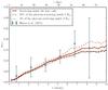 |
Fig. D.2 Effect of the IGM on the polarization profile. We show the polarization profile resulting from the redistribution of all the scattered photons in a sphere of 5 Rvir as a dash-dotted line and the one resulting from the redistribution of all the photons reaching 5 Rvir in a smaller sphere of 2 Rvir as a dotted line. |
In this appendix, we tested a more sophisticated method than in the main text to compute the fraction of photons that will scatter in the IGM beyond the virial radius, inspired from Laursen et al. (2011). It appears that this fraction of scattered photons is even smaller in this scenario. To be conservative in our calculations, we assumed f = 20% in this work, consistent with an average transmission of  for the blue part of the Lyα line, and assuming that the red part of the line is left unchanged by the IGM.
All Tables
All Figures
|
Fig. 1 Two different spectral shapes: a single Gaussian (solid), and a P-Cygni profile (dashed). |
| In the text | |
|
Fig. 2 a) Positions of the young massive stars from which we cast Lyα photons that make up the galactic contribution. b) SB map of the extragalactic emission region. c) SB map of the blob after transfer, with both galactic and extragalactic contribution to Lyα emission. d) Mock observation of the halo with a seeing of 1″. The dashes show polarization, and the contours mark 1.4 × 10⁻¹⁸ erg s-1 cm-2 arcsec-2 and 10-19 erg s-1 cm-2 arcsec-2. |
| In the text | |
|
Fig. 3 Effect of scattering compared to that of a PSF on the observed SB profile for the extragalactic contribution to the luminosity. The SB profiles before (after) transfer are shown in blue (red), the profiles with (without) PSF are represented as a solid (dashed) line. Note that only the emission from extra-galactic gas is taken into account here. |
| In the text | |
|
Fig. 4 Comparison of SB profiles. The red solid line is the SB profile expected from the sum of both gas and galactic contributions; the red dashed lines show the first and third quartiles. The thin orange lines represents the profile for each LOS. The upper (lower) black dotted line shows the the extra-galactic (galactic) contributions. Two observational data taken from the literature (see text box) are shown in blue, data points are H11 observations (teal) and the Matsuda et al. (2012) stacked profile (blue). |
| In the text | |
|
Fig. 5 Polarization radial profiles for a) extragalactic emission; b) galactic emission; and c) the overall Lyα emission. The thin orange lines show the profile corresponding to each LOS; the solid red line is the median profile; the dispersion along different LOS is represented by the two dashed red lines (first and third quartiles). The red area shows the 3σ confidence limits inferred from our bootstrap experiment (see Appendix B). The data points are taken from H11. |
| In the text | |
|
Fig. 6 Distribution of the angle between polarization and tangential direction. The thin orange lines show the profile corresponding to each LOS; the solid red line is the median profile, and the two dashed red lines denote the first and third quartiles. The red area shows the 3σ confidence limits inferred from our bootstrap experiment (see Appendix B), and the teal line is the distribution taken from H11. We show the profile we obtain by assuming some noise in the angle measurement in black. |
| In the text | |
|
Fig. 7 Distribution of the radii of emission, rem, for each observation radius, robs, weighted by the (normalised) luminosity of the photons. These radii are not distances to the halo centre, but projected onto the observation plane perpendicular to the line of sight for each simulated photon. a) Galactic component; b) extragalactic component. |
| In the text | |
|
Fig. 8 Polarization profile obtained by selecting photons according to the distance between the emission and the last scattering. |
| In the text | |
|
Fig. 9 Effect of the IGM on the polarization profile. Compared to the profile right outside of the halo (solid red line), scattering in the IGM (dash-dotted and dotted black lines) reduces slightly the degree of polarization at large radii, but not much (if we redistribute the photons in a large enough area). |
| In the text | |
|
Fig. A.1 Polarization profile for an expanding spherical shell. Results from DL08 are shown in black, our results in red. The solid (dashed) line corresponds to a column density of NH = 1019 cm-2 (NH = 1020 cm-2). |
| In the text | |
|
Fig. B.1 Polarization profile for different subsets of photons. In all the plots, the red solid line is the median profile; the red dashed lines are the first and third quartiles. The thin grey lines represent the profiles for a) 100 LOS with the same photons subset for the gas emission; b) 100 different photon subsets seen with the same LOS for the gas emission; c) 100 LOS with the same photon subsets for the galactic emission; d) 100 different photon subsets seen with the same LOS for the galactic emission. |
| In the text | |
|
Fig. D.1 Left: angle-averaged integrated spectrum of our blob (in black), divided into an extragalactic component (in red) and galactic emission (in blue). Middle: IGM transmission function from Rvir to the observer, fitting the results of Laursen et al. at z = 2.5 (dotted line), z = 3 (solid line) and z = 3.5 (dashed line). Right: resulting spectrum after transmission through the IGM. For all three panels, the vertical line denotes the Lyα wavelength. |
| In the text | |
|
Fig. D.2 Effect of the IGM on the polarization profile. We show the polarization profile resulting from the redistribution of all the scattered photons in a sphere of 5 Rvir as a dash-dotted line and the one resulting from the redistribution of all the photons reaching 5 Rvir in a smaller sphere of 2 Rvir as a dotted line. |
| In the text | |
Current usage metrics show cumulative count of Article Views (full-text article views including HTML views, PDF and ePub downloads, according to the available data) and Abstracts Views on Vision4Press platform.
Data correspond to usage on the plateform after 2015. The current usage metrics is available 48-96 hours after online publication and is updated daily on week days.
Initial download of the metrics may take a while.