| Issue |
A&A
Volume 592, August 2016
|
|
|---|---|---|
| Article Number | A71 | |
| Number of page(s) | 15 | |
| Section | Extragalactic astronomy | |
| DOI | https://doi.org/10.1051/0004-6361/201628676 | |
| Published online | 28 July 2016 | |
HERschel Observations of Edge-on Spirals (HEROES)
III. Dust energy balance study of IC 2531 ⋆,⋆⋆
1 Sterrenkundig Observatorium, Universiteit Gent, Krijgslaan 281, 9000 Gent, Belgium
e-mail: This email address is being protected from spambots. You need JavaScript enabled to view it.
2 St. Petersburg State University, Universitetskij pr. 28, 198504 St. Petersburg, Stary Peterhof, Russia
3 Central Astronomical Observatory of RAS, Pulkovskoye chaussee 65/1, 196140 St. Petersburg, Russia
4 Dipartimento di Matematica e Fisica, Università degli Studi Roma Tre, Via della Vasca Navale 84, 00146 Roma, Italy
5 Department of Physics and Astronomy, University College London, Gower Street, London WC1E 6BT, UK
6 Instituto de Radioastronomía y Astrofísica, CRyA, UNAM, Campus Morelia, A.P. 3-72, 58089 Michoacán, Mexico
7 Department of Physics and Astrophysics, Vrije Universiteit Brussel, Pleinlaan 2, 1050 Brussels, Belgium
8 Instituto de Física y Astronomía, Universidad de Valparaíso, Avda. Gran Bretaña 1111, Valparaíso, Chile
9 Faulkes Telescope Project, Cardiff University, The Parade, Cardiff CF24 3AA, Cardiff, UK
10 Astrophysics Research Institute, Liverpool John Moores University, IC2, Liverpool Science Park, 146 Brownlow Hill, Liverpool L3 5RF, UK
11 Kapteyn Astronomical Institute, University of Groningen, Landleven 12, 9747 AD Groningen, The Netherlands
Received: 8 April 2016
Accepted: 20 May 2016
Abstract
We investigate the dust energy balance for the edge-on galaxy IC 2531, one of the seven galaxies in the HEROES sample. We perform a state-of-the-art radiative transfer modelling based, for the first time, on a set of optical and near-infrared galaxy images. We show that by taking into account near-infrared imaging in the modelling significantly improves the constraints on the retrieved parameters of the dust content. We confirm the result from previous studies that including a young stellar population in the modelling is important to explain the observed stellar energy distribution. However, the discrepancy between the observed and modelled thermal emission at far-infrared wavelengths, the so-called dust energy balance problem, is still present: the model underestimates the observed fluxes by a factor of about two. We compare two different dust models, and find that dust parameters, and thus the spectral energy distribution in the infrared domain, are sensitive to the adopted dust model. In general, the THEMIS model reproduces the observed emission in the infrared wavelength domain better than the popular BARE-GR-S model. Our study of IC 2531 is a pilot case for detailed and uniform radiative transfer modelling of the entire HEROES sample, which will shed more light on the strength and origins of the dust energy balance problem.
Key words: radiative transfer / dust, extinction / galaxies: ISM / infrared: ISM
Herschel is an ESA space observatory with science instruments provided by European-led Principal Investigator consortia and with important participation from NASA.
The reduced images (as FITS files) are only available at the CDS via anonymous ftp to cdsarc.u-strasbg.fr (130.79.128.5) or via http://cdsarc.u-strasbg.fr/viz-bin/qcat?J/A+A/592/A71
© ESO, 2016
1. Introduction
Cosmic dust is one of the fundamental components of the interstellar medium (ISM). Notwithstanding its small contribution to the total mass of a galaxy, interstellar dust plays an important role in many physical and chemical processes in galaxies. It is well established that dust catalyses the transformation of atomic to molecular hydrogen (see e.g. Goldsmith et al. 2007) and contributes to the cooling and heating of the ISM (Tielens 2005). Moreover, dust efficiently absorbs and scatters light at UV and optical wavelengths, and re-emits the absorbed energy as thermal emission at far-infrared (FIR) and submillimeter wavelengths (Soifer & Neugebauer 1991). On average, about one third of all starlight in normal late-type galaxies is absorbed by dust (Popescu & Tuffs 2002; Viaene et al. 2016). A solid knowledge of the amount of dust, its physical properties, its spatial distribution and the heating mechanisms of the interstellar medium are hence crucial for modern astrophysics.
According to the dust energy balance, we would expect the absorbed energy to match the re-emitted energy in the IR/submm domain. However, an inconsistency is generally found: the FIR emission predicted from a model based on extinction at optical wavelengths typically underestimates the observed values by a factor of 3−4. This is the well-known dust energy balance problem that has been observed in many studies (Bianchi et al. 2000; Popescu et al. 2000, 2011; Misiriotis et al. 2001; Alton et al. 2004; Dasyra et al. 2005; Bianchi 2008; Baes et al. 2010; Holwerda et al. 2012; De Geyter et al. 2015).
Edge-on galaxies are of particular interest since these objects offer a unique perspective for studying the vertical, as well as the radial structure, of their stellar components. Moreover, as interstellar dust obscures a large proportion of the emitted starlight, they are ideal targets to study the dusty ISM in spiral galaxies. Both the stellar structure and dust distribution in edge-on galaxies have been considered in multiple studies since the early 1980s (van der Kruit & Searle 1981a; Barteldrees & Dettmar 1994; Xilouris et al. 1999; Pohlen et al. 2000; Kregel et al. 2002; Bianchi 2007; Baes et al. 2010; Mosenkov et al. 2010). In particular, the prototypical edge-on spiral galaxy, NGC 891, has been studied extensively over the past three decades (e.g. van der Kruit & Searle 1981b; Xilouris et al. 1998; Popescu et al. 2000, 2011; Bianchi & Xilouris 2011; Schechtman-Rook et al. 2012; Hughes et al. 2014, 2015). The most suitable approach to derive the intrinsic properties of stars and dust is through dust radiative transfer modelling (for a review, see Steinacker et al. 2013). Several radiative transfer codes now incorporate a full treatment of absorption, multiple scattering, and thermal emission by dust (e.g., Gordon et al. 2001; Baes et al. 2003; Jonsson 2006; Bianchi 2008; Robitaille 2011).
Recently, De Geyter et al. (2015) studied the dust energy balance in two edge-on galaxies, IC 4225 and NGC 5166, observed by Herschel in the frame of the Herschel-ATLAS (Eales et al. 2010). They fitted detailed radiative transfer models directly to a set of optical images and included an additional young stellar disc to match the UV fluxes. They concluded that this additional component is necessary to reproduce the heating of the dust grains. For NGC 5166, the predicted spectral energy distribution (SED) and the model images match the observations very well. However, for IC 4225, the far-infrared emission of their radiative transfer model still underestimates the observed fluxes by a factor of three pointing to the same dust energy problem. One of the possible reasons for this discrepancy could be that the angular size of IC 4225 is too small to properly fit the dust disc parameters. Among the other reasons could be the emission of obscured star-forming regions deeply embedded in dense dust clouds which do not contribute notably to the observed UV flux, but have a clear impact on the FIR emission (see e.g. De Looze et al. 2012, 2014; De Geyter et al. 2015).
In this work, we investigate the dust energy balance in the edge-on galaxy, IC 2531. It is one of the galaxies from the HEROES (Verstappen et al. 2013) sample, a set of seven edge-on spiral galaxies. All of these galaxies have optical diameters of at least 4 arcmin, so that they are well-resolved, even at infrared and submm wavelengths. They were selected as having a clear and regular dust lane, and they have already been fitted with a radiative transfer code based on their optical and near-infrared (NIR) data. All galaxies were observed with the Herschel Space Observatory (Pilbratt et al. 2010), in five bands of the Photodetector Array Camera and Spectrometer (PACS, Poglitsch et al. 2010) and Spectral and Photometric Imaging Receiver (SPIRE, Griffin et al. 2010) at 100, 160, 250, 350, and 500 μm. The general goal of the HEROES project is to present a detailed, systematic, and homogeneous study of the amount, spatial distribution, and properties of the interstellar dust in these seven galaxies, and investigate the link between the dust component and stellar, gas, and dark matter components. The first paper in this series (Verstappen et al. 2013) presented the Herschel imaging data, and the second one (Allaert et al. 2015) presented Hi observations and detailed tilted ring models. The main goals of this third paper is to study the dust energy balance in IC 2531, and to develop an approach that will be used for studying the dust in all HEROES galaxies in a uniform and consistent way.
The outline of this paper is as follows. In Sect. 2, we describe the main properties of IC 2531 taken from the literature. In Sect. 3, we present the available imaging and describe the data reduction. In the following two sections we describe our modelling approach and results (our approach is based on De Geyter et al. 2015, but we use a wider range of imaging data and high-resolution imaging, which forces us to adapt the modelling strategy). In Sect. 4.1, we present a detailed photometrical decomposition of the IRAC 3.6 μm image into several stellar components. In Sect. 4.2, we perform an oligochromatic radiative transfer fitting for this galaxy using seven optical and NIR bands to constrain the main dust disc parameters. The panchromatic radiative transfer modelling of the galaxy based on the retrieved dust and stellar component models is presented in Sect. 5, where we compare different dust mixture models as well. Finally, we discuss our findings in Sect. 6 and present a summary in Sect. 7.
Basic properties of IC 2531.
 |
Fig. 1 Composite RGB-image of the B-, V-, and R-passband frames from the Faulkes Telescope South (see Sect. 3). The length of the white bar in the bottom right corner is 1 arcmin. |
Structural parameters of the stellar and dust components from different studies.
2. The target
IC 2531 is a nearby late-type spiral galaxy (D ≈ 36.8 Mpc; see Table 1) located in the southern hemisphere. It is viewed almost directly edge-on: in Fig. 1 we can see that the sharp dust lane divides the galaxy body into two equal parts. The fitted inclination of  from Xilouris et al. (1999) confirms that it is very close to exactly edge-on. The boxy/peanut-shaped bulge is a prominent detail of this galaxy and has been studied in several works (e.g. Patsis & Xilouris 2006; Bureau et al. 2006), and a slight warp is also visible at optical wavelengths. Despite these peculiarities in the galaxy structure, we choose IC 2531 as a pilot case because it has an overall regular structure and is sufficiently large enough to analyse the observations in the whole UV-submm domain.
A thorough analysis of the Hi content of IC 2531 was carried out by Allaert et al. (2015) as part of the second HEROES paper (see also Kregel et al. 2004; O’Brien et al. 2010a,b). They constructed 3D tilted-ring models of the atomic gas discs of the HEROES galaxies to constrain their surface density distribution, rotation curve, and geometry. For IC 2531, a total Hi mass of 1.37 × 10¹⁰M⊙ was measured. Like the stellar disc, the Hi disc was found to be more extended towards the NE (approaching) side. This side also shows significantly more irregular kinematical behaviour in the Hi data cube than the receding (SW) side. The outer regions of the disc were found to be slightly warped both in the plane of the sky and along the line of sight, with the position and inclination angles deviating by up to about 4 deg with respect to the centre of the galaxy. The best fitting model uses a constant scale height z0 of 1.0 kpc. Within the errors on z0, however, a modest flaring of the gas disc is also possible. Finally, a bright ridge in the major axis Hi position-velocity diagram suggests the presence of a prominent spiral arm in the disc.
The structural parameters of the stellar and dust disc of IC 2531 have already been estimated by several authors (see Table 2). The most advanced modelling was undertaken by Xilouris et al. (1999), who fitted a radiative transfer model to several optical and NIR images. They adopted a model consisting of a double-exponential distribution for the dust and stellar disc plus a de Vaucouleurs profile for the bulge.
The two other works referenced in Table 2 assume a perfectly edge-on orientation of the galaxy. In Kregel et al. (2002), a simple 2D decomposition into a de Vaucouleurs bulge and the double-exponential disc was performed. It is interesting to note that the stellar disc scale length appeared to be twice as large as was found in Xilouris et al. (1999). On the other hand, the bulge is significantly more compact, compared to the same work. These differences of the stellar components may be caused by different fitting techniques or the different quality of the data used in their analysis. Bizyaev & Mitronova (2009) determined both the radial and vertical scale parameters fitting a number of photometrical cuts parallel to the minor axis of the galaxy. Based on the analysis of 2MASS images, they found a model of the stellar disc which is 1.5–2 times thinner than in the previous studies.
A direct comparison of the results from Table 2 is difficult, even at a fixed wavelength, since the different studies used techniques with different levels of sophistication. As demonstrated by Mosenkov et al. (2015), this can seriously affect the resulting galaxy parameters. Particularly striking is the huge discrepancy (more than a factor of two) between the I-band radial scale length obtained by Kregel et al. (2002) compared to the one obtained by Xilouris et al. (1999). The former model seems to be somewhat too simplistic since it does not take into account disc truncation and the attenuation by dust. The latter model, on the other hand, is a full-scale radiative transfer model, which properly takes into account absorption and scattering by interstellar dust.
All in all, the above mentioned studies show that IC 2531 has a more than average radially extended stellar disc (radial scale hR, ∗ ≳ 6 − 8 kpc) with a stronger than average disc flattening (hR, ∗/hz, ∗ ≳ 13) and an extended dust component.
3. Observations and data preparation
Optical observations of IC 2531 were made at the Faulkes Telescope South located at Siding Spring, New South Wales, Australia. The galaxy was observed in the B-, V-, and R-band filters with the 2-m telescope in February 2014. For each band, nine individual images with exposure times of 200 s were cleaned, aligned, and combined into a single science frame using standard data reduction techniques, including bias subtraction, flat-fielding, and removing instrumental artefacts. The final images have a pixel scale of 0.3′′/pix and an average seeing of 1.5′′. A three-colour image combined from all three bands is presented in Fig. 1.
Additional near-infared imaging in the J, H, and Ks passbands was retrieved from the All-Sky Data Release of the Two Micron All Sky Survey (2MASS, Skrutskie et al. 2006). Although the resolution of these images is rather poor, the angular size of the galaxy, along with the signal-to-noise ratio, is sufficient for our further analysis.
Furthermore, we use mid-infrared (MIR) data from the Spitzer Space Telescope (Werner et al. 2004). In this paper we make use of the Infrared Array Camera (IRAC, Fazio et al. 2004), namely 3.6 μm observations available through the Spitzer Heritage Archive (the mosaic *maic.fits and uncertainties *munc.fits files from post-Basic Calibrated Data).
Before the imaging data can be analysed with our methods (see Sects. 4.1 and 4.2), some preparation of the retrieved images is needed. This includes astrometry correction in the same way for all frames, rebinning (i.e. resampling, so that all the data has the same pixel scale), subtraction of the sky background, rotating the images (the galaxy should be aligned with the horizontal axis), cropping the frames to the appropriate size to cover the whole galaxy with very little empty space, and, finally, masking all foreground and background objects that contaminate the galaxy image. In addition, the point spread function (PSF) was carefully determined for all the frames.
To verify the astrometry, we used the astrometric calibration service Astrometry.net1. For the next steps we applied the python Toolkit for skirt2 (pts), which includes special routines to prepare data for the consequent analysis with the fitskirt code. The average alignment of the rebinned images is estimated as being 0.5 pix. Near-infrared observations are strongly affected by thermal radiation from the sky and the telescope, hence, the sky background should be estimated very accurately. To do so, we inspected each frame separately and selected empty parts (using the free software SAOimage DS93) in each frame around the outermost isophotes of the galaxy. The intensities in selected regions were then fitted with a 2nd order polynomial and the fitted sky frames were then subtracted from the respective images. Subsequently, the galaxy images were rotated (the positional angle was measured for the IRAC 3.6 μm image in the way proposed in Martín-Navarro et al. 2012, Sect. 3.1.2), cut out from the initial frames, so that the galaxy 25.5 mag/arcsec2 isophote in the B-band would be fully included. The final images were thoroughly revisited by hand to mask stars, background galaxies, and other contaminants. Finally, we obtained the prepared images of the galaxy in seven bands ready for the fitting analysis. We will call them the reference images since our further modelling is directly based on them.
Apart from the imaging described above, we collected imaging data at other wavelengths, from the far-ultraviolet to the submm. These observations are taken into account during the panchromatic modelling described in Sect. 5. Galaxy Evolution Explorer (GALEX, Martin et al. 2005; Bianchi et al. 2014) observations at 0.152 μm (FUV) and 0.227 μm (NUV) were downloaded from the All Sky Imaging Survey obtainable trough the GalexView service4. IC 2531 was also observed by the Wide-field Infrared Survey Explorer (WISE, Wright et al. 2010), and we downloaded the frames of the galaxy in all four passbands. Herschel imaging was taken from Verstappen et al. (2013), but the reduction was repeated using the latest calibration pipeline.
All the images were prepared in exactly the same way as the reference images, with the same rebinning and alignment. Integrated flux densities for all wavelengths were determined by means of aperture photometry from the photutils python package. We used the same mask for all galaxy images, and the masked areas were filled with the interpolated values using a Gaussian weights kernel. Finally, we added flux densities (APERFLUX) at 353, 545, and 857 GHz (850 μm, 550 μm, and 350 μm, respectively) from the Planck Legacy Archive5 (Planck Collaboration I 2014). The final global fluxes are listed in Table 3.
Observed flux densities and their corresponding errors.
4. Oligochromatic radiative transfer modelling
The first step in our modelling consists of the construction of a radiative transfer model that can reproduce the images at optical (and NIR) wavelengths. The most straightforward approach would be to follow the strategy of De Geyter et al. (2014). They studied a sample of 12 edge-on spiral galaxies, and directly fitted a Monte Carlo radiative transfer model to the SDSS images. Their three-component model consisted of a double-exponential disc to describe the stellar and dust discs and a Sérsic profile to describe the bulge. Though their model contained 19 free parameters, they managed to accurately reproduce almost all the galaxies in the sample, without human intervention or strong boundary conditions.
In this work, we use a different approach. The main driver for this is that, since the HEROES galaxies are so nearby, the images have higher resolution and this three-component model is too simplified. It is well known that the Milky Way has a thin and a thick disc (Gilmore & Reid 1983). Many edge-on galaxies studied within the frame of the S4G project exhibited a clear presence of a thick disc as well (Comerón et al. 2012; Salo et al. 2015). We show later on that IC 2531 can be described more accurately if a model includes a thin and a thick disc rather than one stellar disc. Unfortunately, a model consisting of three stellar components and a dust disc would comprise too many parameters to be fitted directly in a radiative transfer fitting procedure.
Therefore, we decided to use a two-step approach instead of the direct fitting as in De Geyter et al. (2014). First, we use the IRAC 3.6 μm image of IC 2531, for which we can neglect the obscuring effects of dust, to build a geometrical model of the stellar components. Subsequently, we perform an oligochromatic radiative transfer fitting of optical and NIR images with the fixed geometrical parameters of the stellar components (but free luminosity values) and find dust disc parameters. A similar approach was applied to the elliptical galaxy NGC 4370 (Viaene et al. 2015).
4.1. Decomposition of the IRAC 3.6 μm image
The 3.6 μm passband offers a clear view of the old stars of a galaxy, which make up the bulk of the stellar mass. It is not strongly affected by dust extinction and is not sensitive to star-forming regions, making it the best suited band for deriving the structural parameters of the stellar components. Although the resolution of the IRAC 3.6 μm-band image is worse than for the optical images, IC 2531 is still sufficiently resolved in the Spitzer image, providing an opportunity to trace both the thin and thick disc of the galaxy (see below).
The profile of the bulge of a spiral galaxy is usually fitted by means of a Sérsic model (Sérsic 1968): ![Mathematical equation: \begin{equation} I(r) = I_\mathrm{e,b} \: \exp \left\{ -b_n \left[ \left( \frac{r}{r_\mathrm{e,b}} \right)^{1/n_\mathrm{b}} \! - \: 1 \right] \right\}, \end{equation}](/articles/aa/full_html/2016/08/aa28676-16/aa28676-16-eq91.png) (1)where Ie,b is the effective surface brightness, i.e. the surface brightness at the half-light radius of the bulge re,b, and bn is a function of the Sérsic index nb (Caon et al. 1993; Ciotti & Bertin 1999). The apparent axis ratio of the bulge qb is also a free parameter of the model. The 3D luminosity density corresponding to this intensity distribution on the sky can be expressed using complex special functions (Mazure & Capelato 2002; Baes & Gentile 2011; Baes & Van Hese 2011).
(1)where Ie,b is the effective surface brightness, i.e. the surface brightness at the half-light radius of the bulge re,b, and bn is a function of the Sérsic index nb (Caon et al. 1993; Ciotti & Bertin 1999). The apparent axis ratio of the bulge qb is also a free parameter of the model. The 3D luminosity density corresponding to this intensity distribution on the sky can be expressed using complex special functions (Mazure & Capelato 2002; Baes & Gentile 2011; Baes & Van Hese 2011).
To describe the surface brightness distribution of the three-dimensional axisymmetric stellar disc, radiative transfer modellers usually use a 3D luminosity density model where the radial and vertical profile of the luminosity density are exponential (the double-exponential disc). In a cylindrical coordinate system (R,z) aligned with the disc (where the disc mid-plane has z = 0), the luminosity density j(R,z) is given by 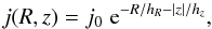 (2)where j0 is the central luminosity density of the disc, hR is the disc scale length, and hz is the vertical scale height. However, analysis of surface brightness profiles of galaxies has shown that not all galactic discs can be described accurately by Eq. (2), since they typically show truncations and anti-truncations (Erwin et al. 2005, 2008; Muñoz-Mateos et al. 2013). A modified profile can be presented as (Erwin et al. 2008; Erwin 2015)
 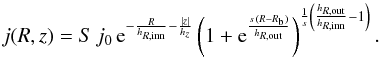 (3)In this formula, s parametrises the sharpness of the transition between the inner and outer profiles with the break radius Rb. We note that the sharpness s is dimensionless, whereas the sharpness parameter α = s/hR,out in Erwin et al. (2008) has units of length-1. Large values of sharpness parameter (s ≫ 1) correspond to a sharp transition, and small values (s ~ 1) set a very gradual break. The dimensionless quantity S is a scaling factor, given by
  (4)Thus, this model contains five free parameters: the scale length of inner disc hR,inn, the scale length of outer disc hR,out, the scale height hz, the break radius Rb, and the sharpness of the break s.
Visual inspection of the minor-axis profile from the IRAC 3.6 μm image for IC 2531 (see Fig. 3, left plot) suggests the presence of both a thin and a thick disc (as an excess over a simple exponential thin disc at the distance | z | ≳ 15″). Also, a slight change of the disc profile slope is visible on the horizontal distribution of the surface brightness at the radius | r | ≈ 120″, which is evidence for the presence of breaks in one or both stellar discs. Therefore, we performed decomposition of the 3.6 μm-band galaxy image into three stellar components: thin and thick discs with breaks plus a central Sérsic component for the bulge.
For this purpose, we used the imfit code which works with the 3D disc and has the BrokenExponentialDisk3D function identical to the model (3) (with n = 100 in Eqs. (40) and (41) in Erwin (2015) to describe the exponential disc model). For PSF convolution, we used an in-flight point response function (PRF) image for the center of the IRAC 3.6 μm field6, downsampled to the 0.6′′ pixel scale and re-rotated to correspond to the analysed galaxy frame. Taking into account that the uncertainty of the galaxy inclination in Xilouris et al. (1999) is small ( ), the disc inclinations in our model were set to be the same for both discs and fixed at
  to minimise the number of free parameters. A fixed sharpness of the breaks, s = 5, was applied for both discs as well. We tried using different values of s (in the range from 0.1 to 100) and found that this parameter does not affect the results of the fitting for this galaxy. We used a genetic algorithm (which is also available in the imfit code) to estimate an initial set of parameters for the model. Subsequently, we ran the Levenberg-Marquardt algorithm to increase the best fitting model.
During the fitting, we found the break radius of the thick disc to be larger than the semi-major axis of the galaxy. Therefore we changed the model for the thick disc to be a simple double-exponential disc without a break. This reduces the number of free parameters even further and, hence, the degeneracy of the fitted model. This is in agreement with Comerón et al. (2012), where it is shown that most thin discs are truncated (77 per cent for their sample of 70 edge-on galaxies, studied within the frame of the S4G project), whereas thick discs are truncated in 31 per cent of the cases.
The results of the fitting are listed in Table 4. As can be seen, the thin disc is the dominant component with the truncation break radius at  , consistent with the results from Comerón et al. (2012; see their Fig. 12). The thick disc is very extended and has very small flattening
  , with a radial scale length ~3.1 times that of the thin disc.
The bulge contributes 19 per cent of the total flux, which confirms that IC 2531 is a late-type galaxy. However, the effective radius is quite large, which can be explained by the extended X-structure in the central part of the galaxy. The moderate Sérsic index n ≈ 2.3 suggests that the bulge lies in the overlapping area between pseudo-bulges and classical bulges (Fisher & Drory 2010). However, low bulge flattening suggests that the central component may appear to be a classical bulge rather than a pseudo-bulge. To disentangle this, a kinematic diagnostic of the inner region is required (Fabricius et al. 2012).
Using two sets of relative mass-to-light ratios ΥT/ Υt = 1.4 and ΥT/ Υt = 2.4 assumed in Comerón et al. (2011), we found the mass ratio  and 0.55, respectively. These values lie on the lower limit of the ranges for
  obtained in their study of thick and thin discs (see Fig. 13 in Comerón et al. 2011). This may indicate that the mass of the thick disc was slightly underestimated. However, this issue does not strongly affect our conclusions since the dust model parameters should not be substantially sensitive to the thick disc fraction to the total stellar model (see Sect. 5.1).
In Fig. 2 we can see the reference image, the model, and the residual image for IC 2531. Our model fit is very satisfactory, with the relative difference between the observation and the model below 25 per cent. Only the sharp X-structure in the centre slightly deviates from the model. The vertical and horizontal profiles in Fig. 3 are almost perfectly described by the model. We can see that the thick disc begins to dominate at large radii of the galaxy and has a very low surface brightness, compared to the thin disc.
In summary, we conclude that our galaxy model follows the observations very well and can be used for the subsequent analysis of the dust in the galaxy.
Results of the decomposition of the IRAC 3.6 μm image for IC 2531.
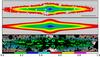 |
Fig. 2 IRAC 3.6 μm image (top), best fitting image (middle) and residual image, which indicates the relative deviation between the fit and the image in absolute values (bottom). The length of the bar on the top plot corresponds to 1 arcmin. The bottom color bar shows the scaling of the residual maps. |
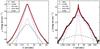 |
Fig. 3 Vertical profile summed up in the range of | r | ≥ 50″ where the fraction of the bulge is neglected (left) and horizontal profile summed up over all pixels in z-direction (right). |
4.2. FITSKIRT fitting
To build a realistic model for a dusty edge-on galaxy, we use the model obtained in Sect. 4.1 to describe the stellar components of the galaxy, plus a dust disc represented by the double-exponential disc (see e.g. Xilouris et al. 1999; Baes et al. 2010; Verstappen et al. 2013; De Geyter et al. 2013, 2014):  (5)where Md is the total dust mass, and hR,d and hz,d are the radial scale length and vertical scale height of the dust, respectively. The central face-on optical depth, often used as an alternative to express the dust content, is found as
 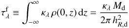 (6)where κλ is the extinction coefficient of the dust. The central edge-on optical depth can be found to be
  .
.
As discussed in the previous subsection, we fix the geometry of the different stellar components in the radiative transfer modelling, and we only fit the parameters of the dust disc, plus the centre alignment, the inclination angle i, and position angle PA (even though we have aligned the galaxy plane with the horizontal axis, this alignment can still have a little error). Even though there is evidence that disc scale lengths are wavelength dependent (Peletier et al. 1994; Corradi et al. 1996; Xilouris et al. 1999), the 3.6 μm surface brightness distribution best traces the stellar distribution of the galaxy, and we expect that our fixed geometrical model to be satisfactorily applicable at optical wavelengths as well. We note that we use the same geometrical parameters at all wavelengths for the dust disc and that only the luminosities of the bulge and the stellar discs are determined individually at each wavelength. This simulates the wavelength-dependent behaviour of their luminosity ratios (De Geyter et al. 2013, 2014). We also note that, at this stage, we do not make any assumptions about the characteristics of the stellar populations. We just fit the emission in every band individually and scale the emission without making assumptions about how the emission in different wavebands is linked. This approach allows as to significantly reduce the number of fitted parameters and, at the same time, use a complex model to describe the stellar and dust components of the galaxy.
To describe our dust model, we should specify the optical properties of dust such as the absorption efficiency, the scattering efficiency, and the scattering phase function. We initially use the standard BARE-GR-S model described in Zubko et al. (2004) and implemented as in Camps et al. (2015). This model consists of a mixture of polycyclic aromatic hydrocarbons (PAHs), graphite, and silicate grains. The relative distributions of each grain component have been weighted to best match the extinction, abundances, and emission associated with the Milky Way dust properties (Rv = 3.1). We note that the skirt code considers individual silicate, graphite, and polycyclic aromatic hydrocarbon grain populations for the calculation of the dust emission spectrum, and that it fully takes into account the transient heating of PAHs and very small grains (Camps et al. 2015), using techniques described in Guhathakurta & Draine (1989) and Draine & Li (2001).
To fit the galaxy images described in Sect. 3 with the model described above, we applied the oligochromatic radiative transfer-fitting code fitskirt (De Geyter et al. 2013, 2014). fitskirt is a fitting code built around the 3D Monte Carlo radiative transfer code skirt (Baes et al. 2003, 2011; Camps & Baes 2015)7. Our 3D model should reproduce the observed optical/NIR images of the galaxy, fully taking into account the effects of absorption and multiple anisotropic scattering by dust. fitskirt determines the best-fit parameters for the 3D distribution of stars and dust using genetic algorithm-based optimisation. Since the Monte Carlo method inevitably produces some Poisson noise, traditional optimisation tools, such as Levenberg-Marquardt’s algorithm, are not applicable in this case. Genetic algorithms, which have been successfully applied to a wide range of global optimisation problems, can easily handle noisy objective functions (Metcalfe et al. 2000; Larsen & Humphreys 2003; De Geyter et al. 2013).
For this work, some new features have been added to the fitskirt code. The code can now work with an arbitrary combination of stellar and dust components. A further improvement is that arbitrary PSF kernels can be provided, rather than the Gaussian kernels that were assumed in previous versions. The PSF is to be provided as a separate image, which can can be a cut out of an unsaturated star with high signal-to-noise ratio, or a model Gaussian or Moffat function. In case of images from space telescopes with very sophisticated PSF, this new accurate PSF convolution is vital for retrieving reliable parameters of stellar components.
First, we performed oligochromatic fitting of the three images in the B, V and R-bands. After that, we repeated the same fitting but for seven bands: the same optical B-, V-, and R-band images plus four NIR images in the J, H, Ks and IRAC 3.6 passbands. The computations are done using the high performance cluster of the Flemish Supercomputer Center (Vlaams Supercomputer Centrum). To estimate the uncertainties of the parameters, we repeated the fitting five times for the models based on three as well as seven band images.
The results of the fitting for both cases (best fits) are listed in Table 5. As can be seen, the model built upon the seven bands is significantly better constrained than the model based on only the optical images. Although the dust mass is almost the same, its uncertainty is very large in the first case, whereas the relative errors on each of the derived parameters for the second model are very small. In the first fit, the dust disc appears less extended and slightly thinner, which leads to a larger optical thickness. We will use the seven band model for our next analysis in Sect. 5.
Results of fitskirt fitting for IC 2531.
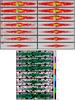 |
Fig. 4 Results of the oligochromatic fitskirt radiative transfer fits for IC 2531. In each panel, the top left-hand column represents the observed image, the top right-hand column contains the corresponding fits in the same bands, the bottom column shows the residual images, which indicate the relative deviation between the fit and the image. |
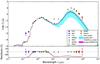 |
Fig. 5 SEDs of IC 2531 with the BARE-GR-S dust mixture based on the BVR fit (black solid line) and the BVRJHK3.6 fit (red dashed line). The coloured markers with error bars correspond to the flux densities listed in Table 3. The bottom panel below the SEDs shows the relative residuals between the observed SEDs and the models. The cyan spread corresponds to the BVR fit and the magenta spread relates to the BVRJHK3.6 fit. The spreads are plotted for the models within one error bar of the best oligochromatic fitting model parameters. |
The reference images (top left), models (top right) and the residual images (bottom) for the best fitting model are presented in Fig. 4. The fitskirt model reproduces the images quite accurately. One can see that the residuals show very little deviation in all passbands with slightly visible traces of the dust lane, especially where the disc has a perceptible warp and/or a possible spiral structure. The most prominent feature in the residual maps is the X-shaped pattern in the centre which cannot be fitted with our simple Sérsic bulge.
The dust scale height of 0.25 kpc and the dust radial length of 8.44 kpc are in remarkable agreement with the average values 0.25 kpc and 8.54, respectively, found with fitskirt for 12 galaxies from the CALIFA sample (De Geyter et al. 2014). However, the dust disc scales listed in Table 2 taken from Xilouris et al. (1999) are 50 per cent larger than presented here. Also, the face-on optical depth in the V-band from our fit is a factor of two larger than found in the same work. However, the large edge-on optical depth in the V-band from our model is consistent with the average value of 19.09 for the sample from De Geyter et al. (2014). We should note that Xilouris et al. (1999) used a different model with a single stellar disc and a de Vaucouleurs’ profile for the bulge, therefore a direct comparison in this case is impossible. In addition, while the skirt code uses a complete treatment of absorption and multiple anisotropic scattering, Xilouris et al. (1999) use an approximate radiative transfer algorithm in which higher order scatterings are approximated (see Kylafis & Bahcall 1987; Xilouris et al. 1997, for details).
5. Panchromatic radiative transfer modelling
In this section, we extend the oligochromatic models obtained in Sect. 4.2 to panchromatic models that can reproduce not only the images at optical and near-infared wavelengths, but also explain the entire UV-submm SED (Table 3). In addition, this enables us to compare the predicted model images with corresponding observations at different wavelengths. This helps us to see how well our model can reproduce the visible structure of the galaxy and draw some conclusions from that.
5.1. Initial model
First, we directly use the earlier obtained oligochromatic fitskirt model (see Sect. 4.2) to predict the view of the galaxy in the entire UV to submm domain. This implies that both the properties for the stars and dust need to be set over this entire wavelength domain. For the stellar components, we assume a Bruzual & Charlot (2003) single stellar population SED with a Chabrier (2003) initial mass function and a solar metallicity (Z = 0.02). We coarsely determined the mass-weighted ages of the stellar components using their de-reddened fluxes retrieved from the fitskirt modelling. For this, we used an adapted version of the SED fitting tool from Hatziminaoglou et al. (2008, 2009). We found that the ages of both the thin and the thick discs are about 5 Gyr and about 8 Gyr for the bulge. For the Milky Way, the thick disc is primarily made of old and metal-poor stars compared to the thin stellar population (Reid & Majewski 1993; Chiba & Beers 2000). This should be the case for IC 2531 as well. However, since the thick disc is more extended in the vertical direction and faint in the dust disc plane (the thick disc-to-dust disc scale height ratio is larger than 6), its influence on the dust emission in the infrared should be minimal.
In Sect. 4.2 we considered two models: one based only on the optical B, V, and R images, and another one based on the optical and NIR images. The black line in Fig. 5 is the predicted SED corresponding to the former model (the SED was normalised to match the V-band luminosity). The model reproduces the observed SED very well in the optical and NIR bands, the model fluxes match the observations very well, even though it is only based on optical images. The agreement is much poorer outside this range: the model SED underestimates the observed flux densities in the UV and the dust emission in the MIR-submm region. The cyan coloured band indicates the spread of the model SED, generated according to the error bars of the dust parameters presented in Table 5. Since some of the parameters are constrained relatively weakly, the spread is significant.
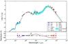 |
Fig. 6 SED of IC 2531 based on the BARE-GR-S (the dashed line) and THEMIS (the solid line) dust mixture, with an additional young stellar component. The coloured symbols with error bars correspond to the flux densities listed in Table 3. The cyan band represents the spread in the MIR and FIR emission of the THEMIS model with different values of the scale height of the young stellar population (see text). The bottom panel below the SED show the relative residuals between the observed SED and the models. |
The red line in Fig. 5 corresponds to the fitskirt model based on the BVRJHK3.6 photometry, with the well-constrained dust parameters. We refer only to this oligochromatic model from now on since it is much better constrained and built on the NIR as well as the optical photometry. The panchromatic simulations are performed in accordance with what was done above, except that the entire SED is normalised to match the IRAC 3.6 μm-band luminosity. The SEDs for both models have very similar behaviour and are almost indistinguishable from each other. However, the spread of possible flux density values for the BVRJHK3.6-based model (magenta colour) is barely visible. Nevertheless, the same underestimation of the UV and dust emission fluxes is present.
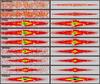 |
Fig. 7 Comparison between the observations (left) and model images (right). |
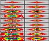 |
Fig. 7 continued. |
5.2. Models with an additional young stellar population
From Fig. 5, it is evident that we need an additional source of UV luminosity, i.e., a young stellar component, to match the observed SED of IC 2531. As UV radiation is easily absorbed by interstellar dust, the addition of an additional young population will also affect the dust emission at MIR-submm wavelengths as well.
According to recent studies of the Milky Way (Jurić et al. 2008; McMillan 2011), the thickness of the thin disc is 200–300 pc, whereas the scale height of the young stellar disc which consists of OB-associations is about 50 pc (Bahcall & Soneira 1980; Bobylev & Bajkova 2016). Moreover, the thickness of young stellar populations in spiral galaxies is similar or smaller than the dust disc scale height (Schechtman-Rook & Bershady 2013, 2014). In our models, for the young stellar disc, we assume a scale height of 100 pc and the same scale length of 8 kpc as for the thin disc. As shown by De Looze et al. (2014) and De Geyter et al. (2015), ranging the thickness of the young stellar disc between one third of the dust scale height to one dust scale height barely affects the resultant SED. Nevertheless, we consider a possible influence of varying the thickness of the young stellar population on the model SED in Sect. 5.3.
The observed GALEX FUV image traces unobscured star formation regions of the galaxy. The stellar emission spectrum of these stars is described through a starburst99 SED template that represents a stellar population with a constant, continuous star formation rate (SFR) and an evolution of up to 100 Myr (Leitherer et al. 1999). In this case, the initial mass function is a Salpeter (1955) IMF with masses between 1 and 100 M⊙ and with solar metallicity. The luminosity of this component is constrained by the GALEX FUV flux density.
The simulated SED of this updated model is shown in Fig. 6 (red dashed line). As can be seen, the contribution of this young stellar population is negligible in the optical and NIR bands, while, on the other hand, it describes the MIR/FIR region significantly better compared to the previous model without the inclusion of the young stellar population. The WISE W3 flux is perfectly reproduced, whereas the PACS 100 μm flux is underestimated by about 25 per cent. At the same time, the model overestimates the observed WISE 22 μm flux density by more than 70 per cent, whereas it significantly underestimates the observed flux densities beyond 100 μm. We should also point out that the model appears to underestimate the observed NUV flux as well. This could be linked to our choice of the dust model: while extinction curves of different galaxies tend to agree well at optical wavelengths, they show quite some diversity in the UV, in particular around the 2175 Å bump (e.g., Gordon et al. 2003).
5.3. THEMIS dust model
In Sect. 5.2 we showed that the Zubko et al. (2004) BARE-GR-S model overestimates the MIR and underestimates the submm flux densities of IC 2531. We decided to verify whether these discrepancies are related to the adopted dust model. To this end, we replace the BARE-GR-S dust model with the so-called THEMIS dust model presented by Jones et al. (2013) and Köhler et al. (2014, 2015). This model is built completely on the basis of interstellar dust analogue material that has been synthesised, characterised, and analysed in the laboratory. In this model, there are two families of dust particles: amorphous carbon and amorphous silicates. For the silicates, it is assumed that 50 per cent of the mass is amorphous enstatite, and that the remaining half is amorphous forsterite.
The same simulations as in the previous Sect. 5.2 were carried out. We used exactly the same model for the stellar components and the dust disc parameters, with the additional young stellar population. The only difference was the dust composition, which was changed to the THEMIS dust model. In Fig. 6 (the black solid line), the model reproduces the MIR/FIR SED region better than that with the BARE-GR-S dust implementation, especially at WISE 22 μm, SPIRE, and Planck wavelengths. However, the comparison between the model and the observations is still not fully satisfactory. A substantial FIR excess remains: the model dust emission appears to be underestimated by a factor of 2.
The cyan spread in Fig. 6 is related to the models with maximal and minimal dust emission and takes into account two aspects. First, it includes the uncertainty of the measured FUV flux density. Second, we varied the disc thickness of the young stellar population from 50 pc to 150 pc (in fact, we found this variance of the disc thickness had a minor affect on the SED). It is seen that the difference in the SED is notable in the MIR/FIR region up to λ ≲ 200 μm, whereas for the cold dust the difference is negligibly small.
It is interesting to compare the SEDs for the THEMIS and BARE-GR-S dust models, which are both presented in Fig. 6. We can see the main difference in the MIR-submm domain. The THEMIS model overestimates the WISE W3 flux and fully restores the WISE W4 flux, whereas for the BARE-GR-S model, we see the contrary result at the same wavelengths. The THEMIS model (together with its spread) accounts for the PACS 100 μm flux density and produces more dust emission in the FIR/submm region compared to the BARE-GR-S model. We discuss this result in Sect. 6.
5.4. Comparing the observed and simulated images
In Fig. 7, we compare a set of images corresponding to the THEMIS dust model described in Sect. 5.3 to the reference images in different bands across the entire wavelength range, from the UV to the submm. The modelled images have been convolved with the appropriate point spread function: for FTS, 2MASS and IRAC 3.6 μm we used the PSFs built in Sect. 3, for the other bands we used the kernels provided by Aniano et al. (2011).
The GALEX FUV image is too noisy to be compared, and we provide it here only for completeness. The GALEX NUV image is better comparable, but still the deepness of the image is not sufficient to do a reliable analysis of it. Nevertheless, we can see that the 2D profile of the simulated image resembles the observed one, though the vertical surface brightness distribution in the observed image seems wider. In an attempt to remedy the situation with the low signal-to-noise ratio of the observed image, we fitted the vertical profile summed over all radii with an exponential function and estimated its scale height hz = 531 ± 7 pc, whereas, for the simulated NUV image, we obtained hz = 215 ± 3 pc. This UV excess can be explained by the presence of another, more vertically extended young stellar component. Alternatively, it could be diffuse scattered light produced by a radially extended PSF (Sandin 2014) or scattered emission from a vertically extended dust distribution (see e.g. Hodges-Kluck & Bregman 2014; Shinn & Seon 2015; Baes & Viaene 2016).
The next set of simulated images, from the FTS B band to the WISE W2 band, are in very good agreement with the observations. However, the periphery of the galaxy disc exhibits prominent flaring (an apparent increase of the disc thickness with radius). This could be due to real physical flaring or the projection of disc warps, or the specific orientation of spiral arms towards the observer.
In the images from WISE W3 to PACS 100 μm, the signature of this spiral structure is visible. In Fig. 8, we present the comparison of two models for IC 2531 taken from Allaert et al. (2015). Both the top and bottom plots represent the WISE W3 image, overplotted with the observed Hi contours (black) and the white contours for a model that does not contain spiral arms (top) and a toy model that includes arcs to mimic the effect of spiral arms in the position-velocity diagram (bottom). This comparison shows that spiral arms could indeed explain the overdensities seen in the WISE W3 image. Spiral arms are probable also present in the other PACS and SPIRE images (the dust emission component is more radially extended, compared to the modelled one), but the spatial resolution at those wavelengths is not sufficient to draw strong conclusions. Also, one can see that the profile of the observed structure at these wavelengths has a rounder shape in comparison with the model that looks more discy. Again, this discrepancy may be related to the presence of a spiral structure, which can widen the vertical distribution of the surface brightness along the major axis of the galaxy. As has been mentioned before, the SPIRE images appear about twice as luminous than the simulations.
 |
Fig. 8 Comparison of two models from Allaert et al. (2015) without (top plot) and with arcs mimicking the effect of spiral arms (bottom plot), built on the basis of the kinematical information analyzed in their work. For both plots, the WISE W3 image is overplotted with the observed Hi contours (black) and the contours from a model (white). Contour levels are 1.49 × 10²¹, 4.475 × 10²¹ and 6.56 × 10²¹ atoms cm-2. |
In general, our simulations seem to match the observations reasonably well, except for the FIR/submm wavelengths, where the galaxy geometry is more complex and the total fluxes are underestimated by a factor of about 2.
6. Discussion
6.1. The need for oligochromatic fitting
As shown in Sect. 5.1, the uncertainties in the dust disc parameters can be dramatically affected by the data that are taken into account: the optical+NIR based data model is much more constrained than the model where only the optical images are fitted. This is similar to what was found by De Geyter et al. (2014), where they validate the oligochromatic fitting procedure on simulated images. They show that oligochromatic models have smaller error bars on most of the fitted model parameters than the individual monochromatic models. In our case of a real galaxy, we can see that the uncertainty of the model can be substantial, even if we do oligochromatic fitting of optical data in several bands. For a more precise model, NIR data is needed. Evidently, the more data we use, on a larger scale of wavelengths, the better constrained our model will be which, in principal, should predict a more consistent SED behaviour at other wavelengths.
The result that adding NIR images significantly constrains the dust model should be discussed. First, let us turn to the work by De Geyter et al. (2014), where they analysed a sample of 12 edge-on spiral galaxies. For this, they used g-, r-, i- and z-band images from the Sloan Digital Sky Survey (Ahn et al. 2014) to perform fitskirt oligochromatic fitting with a model consisting of a double exponential stellar disc, a bulge and an exponential disc for the dust component. In general, the dust parameters they retrieved from their fitting are quite well constrained. For a few galaxies, however, the error bar on the dust mass was up to 50 percent. There are various reasons for such large uncertainties. First, the simple stellar model, consisting of a bulge and an exponential disc, does not accurately describe the observed morphology of the galaxy. Second, using an exponential disc model can be a too simplified model if dust in the galaxy is distributed in a more complex way. Third, the large uncertainties of the dust model can be explained by an insufficient angular resolution of the images used for the galaxy fitting.
In the case of IC 2531, it is unlikely that any of the above cause the large uncertainties on the dust parameters for the BVR model. We have seen that our stellar model describes the observations very well. Also, the exponential disc model for the dust seems to be reasonable. The emission coming from an extended structure in the PACS and SPIRE images is likely related to the spiral structure. In addition, the BVR images used for the fitskirt modelling are sufficiently large compared to the images of the galaxies fitted in De Geyter et al. (2014).
A possible explanation of the poorly constrained dust disc for the BVR-based model might be due to the fact that we have set the geometry of the stellar components for the optical images based on the observed IRAC 3.6 μm images. The actual geometry of the stellar components at optical wavelengths could be different, since stellar populations of different ages dominate at different wavelengths. As mentioned in Sect. 4.1, however, direct fitting of galaxy images with a complex model consisting of three stellar components and a dust disc, is too ambiguous a computational task. Our approach of using a NIR galaxy image for building the stellar model (and adopting it at all wavelengths) seems to be the only possible solution to avoid this issue.
There is another concern related to the dust model constraints. Since NIR images are not strongly affected by dust extinction, it is not evident why adding NIR images in fitting should constrain the dust model parameters. Nevertheless, if we look at the SEDs for the BVR and BVRJHK3.6 models (see Fig. 5), we can see that the spread for the former is negligible in the J-band and becomes gradually larger at longer wavelengths: the uncertainty of the flux density at 3.6 μm is about 20 per cent of the observed value, whereas it is about 9 per cent for the J-band. Moreover, the significant spread for the BVR-based model at 3.6 μm shows that, in fact, the dust model may non-negligibly affect the total flux in this band. Indeed, even rather opaque models (up to  ) are possible within the range of dust parameters. However, if we fit optical and NIR data, our model SED becomes significantly better constrained at the considered wavelengths, which subsequently constrains the dust model and the predicted SED at other wavelengths.
6.2. The dust model
In Sect. 5.3, we compared two physical dust models: the standard BARE-GR-S model from Zubko et al. (2004) versus the THEMIS dust model by Jones et al. (2013) and Köhler et al. (2014, 2015). It is apparent that including the Herschel PACS and SPIRE data should set constraints on both the warm and cold dust components. However, these two different dust models result in different dust emission SEDs: compared to the BARE-GR-S model, the THEMIS model produces less MIR emission, but more emission at FIR and submm wavelengths. This difference can be explained by the fact that the dust grains in these models have different optical and calorimetric properties, which apparently leads to, on average, cooler dust for the THEMIS model.
Fanciullo et al. (2015) compared several dust models in reproducing dust emission and extinction for Galactic diffuse ISM observations from the Planck, IRAS and SDSS surveys. They find that the THEMIS model better matches observations than the Draine & Li (2007) and Compiègne et al. (2011) models. Also, it produces more emission in the far-infrared and submillimeter domain, while “astronomical silicate” and graphite are not emissive enough in that region.
In summary, we can conclude that the excess of the SED (data – model) strongly depends on the adopted dust mixture model. The question of which model, from a physical point of view the more appropriate to use, is still debatable, although for IC 2531 the THEMIS model seems to provide the results which are in better agreement with the observations. We will compare these dust mixtures for the remaining HEROES galaxies in our next study. Obviously, the choice of the dust model can be one of the sources of the dust energy balance problem.
6.3. The dust energy balance and the HEROES sample
The dust energy balance problem for IC 2531 is not completely solved in this paper. However, we have shown that the dust mixture model plays an important role in shaping the model SED.
With time, this problem seems to become more complicated as several possible solutions are being proposed, but none of them can be considered as dominant. A possible explanation is the presence of additional dust distributed in the form of a second inner disc that hardly contributes to the galaxy attenuation, but still provides a considerable fraction of the FIR emission (Popescu et al. 2000; Misiriotis et al. 2001; Popescu et al. 2011). As recently shown by Saftly et al. (2015), complex asymmetries and the inhomogeneous structure of the dust medium may help to explain the discrepancy between the dust emission predicted by radiative transfer models and the observed emission in energy balance studies for edge-on spiral galaxies. Another source of the infrared excess can be completely obscured star-forming regions (see e.g. De Looze et al. 2014; De Geyter et al. 2015). It is quite possible that this problem encompasses several mechanisms that may work at the same time.
As advocated by De Geyter et al. (2015) and Saftly et al. (2015), the best way to discriminate between the various possible explanations (or estimate their contribution) is to select a sample of galaxies with a rich data set and model them in a uniform way. Apart from being a detailed study of IC 2531, already an interesting and well-studied galaxy, a second goal of this paper was to develop a modelling approach that can be applied to a larger set of galaxies. We will apply the approach presented in this work to all HEROES galaxies. Stellar components for each object will be determined from NIR images, taking into account thin and thick discs if appropriate. The dust component will be modelled with fitskirt, by simultaneously analyzing images in a number of optical and NIR bands. This analysis will provide us with a 3D model for each galaxy, including their geometry and masses of stellar and dust components. Taking into account additional data ranging from UV to submm wavelengths, we will be able to construct model SEDs, compare them with observations and make a quantitative assessment of the dust energy balance problem for each galaxy. Also, we will investigate the detailed distribution of dust in all HEROES galaxies and obtain some statistics of dust properties on the basis of the performed analysis, which can be compared to previous works. Models of stellar components will be used in our next study of dynamical properties of the HEROES galaxies.
7. Summary
We have explored the distribution of stars and dust, and the dust energy balance of the edge-on spiral galaxy IC 2531 using the available observations from UV to submm wavelengths. We have expanded the modelling method of De Geyter et al. (2015) to a three-step approach. We first constructed a detailed parametric model for the stellar components, based on a decomposition of the IRAC 3.6 μm image. Then, we carried out an oligochromatic radiative transfer fitting of the optical plus NIR data, to retrieve the dust content parameters. Finally, we expanded this model to a panchromatic model and predicted the resulting SED over the entire UV-submm wavelength domain.
The main findings of this article can be summarised as follows:
-
1.
We manage to build a radiative transfer model that accuratelyreproduces the observed images of IC 2531 atoptical and NIR wavelengths. The structural parameters are ingood agreement with previous studies of other edge-on spiralgalaxies.
-
2.
Even when adding an additional young stellar disc to the model to fit the UV flux densities, the radiative transfer model underestimates the observed far-infrared emission by a factor of a few.
-
3.
Adding NIR imaging to the optical data in the oligochromatic fitting significantly constrains the parameters of the dust distribution.
-
4.
Different dust models, such as the BARE-GR-S and THEMIS dust models used in this work, produce slightly different SEDs. This might be important when determining the nature of the dust energy balance problem.
The latest version is available at http://www.skirt.ugent.be/pts/
skirt and fitskirt are publicly available. The latest version can be downloaded from the official skirt web site http://www.skirt.ugent.be
Acknowledgments
A.V.M. is a beneficiary of a postdoctoral grant from the Belgian Federal Science Policy Office, and also expresses gratitude for the grant of the Russian Foundation for Basic Researches number 14-02-00810 and 14-22-03006-ofi. F.A., M.B., I.D.L. and S.V. gratefully acknowledge the support of the Flemish Fund for Scientific Research (FWO-Vlaanderen). M.B. acknowledges financial support from the Belgian Science Policy Office (BELSPO) through the PRODEX project “Herschel-PACS Guaranteed Time and Open Time Programs: Science Exploitation” (C90370). T.M.H. acknowledges the CONICYT/ALMA funding Program in Astronomy/PCI Project No. 31140020. J.V. acknowledges support from the European Research Council under the European Union’s Seventh Framework Programme (FP/2007−2013)/ ERC Grant Agreement No. 291531. This work was supported by CHARM and DustPedia. CHARM (Contemporary physical challenges in Heliospheric and AstRophysical Models) is a phase VII Interuniversity Attraction Pole (IAP) program organized by BELSPO, the BELgian federal Science Policy Office. DustPedia is a collaborative focused research project supported by the European Union under the Seventh Framework Programme (2007−2013) call (proposal No. 606847). The participating institutions are: Cardiff University, UK; National Observatory of Athens, Greece; Ghent University, Belgium; Université Paris-Sud, France; National Institute for Astrophysics, Italy and CEA (Paris), France. The Faulkes Telescopes are maintained and operated by Las Cumbres Observatory Global Telescope Network. We also thank Peter Hill and the staff and students of College Le Monteil ASAM (France), The Thomas Aveling School (Rochester, England), Glebe School (Bromley, England) and St David’s Catholic College (Cardiff, Wales). This work is based in part on observations made with the Spitzer Space Telescope, which is operated by the Jet Propulsion Laboratory, California Institute of Technology under a contract with NASA. This publication makes use of data products from the Two Micron All Sky Survey, which is a joint project of the University of Massachusetts and the Infrared Processing and Analysis Center/California Institute of Technology, funded by the National Aeronautics and Space Administration and the National Science Foundation. This publication makes use of data products from the Wide-field Infrared Survey Explorer, which is a joint project of the University of California, Los Angeles, and the Jet Propulsion Laboratory/California Institute of Technology, funded by the National Aeronautics and Space Administration. This study makes use of observations made with the NASA Galaxy Evolution Explorer. GALEX is operated for NASA by the California Institute of Technology under NASA contract NAS5-98034. The Herschel spacecraft was designed, built, tested, and launched under a contract to ESA managed by the Herschel/Planck Project team by an industrial consortium under the overall responsibility of the prime contractor Thales Alenia Space (Cannes), and including Astrium (Friedrichshafen) responsible for the payload module and for system testing at spacecraft level, Thales Alenia Space (Turin) responsible for the service module, and Astrium (Toulouse) responsible for the telescope, with in excess of a hundred subcontractors. SPIRE has been developed by a consortium of institutes led by Cardiff Univ. (UK) and including: Univ. Lethbridge (Canada); NAOC (China); CEA, LAM (France); IFSI, Univ. Padua (Italy); IAC (Spain); Stockholm Observatory (Sweden); Imperial College London, RAL, UCL-MSSL, UKATC, Univ. Sussex (UK); and Caltech, JPL, NHSC, Univ. Colorado (USA). This development has been supported by national funding agencies: CSA (Canada); NAOC (China); CEA, CNES, CNRS (France); ASI (Italy); MCINN (Spain); SNSB (Sweden); STFC, UKSA (UK); and NASA (USA). We acknowledge the use of the ESA Planck Legacy Archive. Some of the data presented in this paper were obtained from the Mikulski Archive for Space Telescopes (MAST). STScI is operated by the Association of Universities for Research in Astronomy, Inc., under NASA contract NAS5-26555. Support for MAST for nonHST data is provided by the NASA Office of Space Science via grant NNX13AC07G and by other grants and contracts. This research makes use of the NASA/IPAC Extragalactic Database (NED) which is operated by the Jet Propulsion Laboratory, California Institute of Technology, under contract with the National Aeronautics and Space Administration, and the LEDA database (http://leda.univ-lyon1.fr).
References
- Ahn, C. P., Alexandroff, R., Allen de Prieto, C., et al. 2014, ApJS, 211, 17 [NASA ADS] [CrossRef] [Google Scholar]
- Allaert, F., Gentile, G., Baes, M., et al. 2015, A&A, 582, A18 [NASA ADS] [CrossRef] [EDP Sciences] [Google Scholar]
- Alton, P. B., Xilouris, E. M., Misiriotis, A., Dasyra, K. M., & Dumke, M. 2004, A&A, 425, 109 [NASA ADS] [CrossRef] [EDP Sciences] [Google Scholar]
- Aniano, G., Draine, B. T., Gordon, K. D., & Sandstrom, K. 2011, PASP, 123, 1218 [NASA ADS] [CrossRef] [Google Scholar]
- Baes, M., & Gentile, G. 2011, A&A, 525, A136 [NASA ADS] [CrossRef] [EDP Sciences] [Google Scholar]
- Baes, M., & Van Hese, E. 2011, A&A, 534, A69 [NASA ADS] [CrossRef] [EDP Sciences] [Google Scholar]
- Baes, M., & Viaene, S. 2016, A&A, 587, A86 [NASA ADS] [CrossRef] [EDP Sciences] [Google Scholar]
- Baes, M., Davies, J. I., Dejonghe, H., et al. 2003, MNRAS, 343, 1081 [NASA ADS] [CrossRef] [Google Scholar]
- Baes, M., Fritz, J., Gadotti, D. A., et al. 2010, A&A, 518, L39 [NASA ADS] [CrossRef] [EDP Sciences] [Google Scholar]
- Baes, M., Verstappen, J., De Looze, I., et al. 2011, ApJS, 196, 22 [NASA ADS] [CrossRef] [Google Scholar]
- Bahcall, J. N., & Soneira, R. M. 1980, ApJS, 44, 73 [NASA ADS] [CrossRef] [Google Scholar]
- Barteldrees, A., & Dettmar, R.-J. 1994, A&AS, 103, 475 [NASA ADS] [Google Scholar]
- Bianchi, S. 2007, A&A, 471, 765 [NASA ADS] [CrossRef] [EDP Sciences] [Google Scholar]
- Bianchi, S. 2008, A&A, 490, 461 [NASA ADS] [CrossRef] [EDP Sciences] [Google Scholar]
- Bianchi, S., & Xilouris, E. M. 2011, A&A, 531, L11 [NASA ADS] [CrossRef] [EDP Sciences] [Google Scholar]
- Bianchi, S., Davies, J. I., & Alton, P. B. 2000, A&A, 359, 65 [NASA ADS] [Google Scholar]
- Bianchi, L., Conti, A., & Shiao, B. 2014, Adv. Space Res., 53, 900 [Google Scholar]
- Bizyaev, D., & Mitronova, S. 2009, ApJ, 702, 1567 [NASA ADS] [CrossRef] [Google Scholar]
- Bobylev, V. V., & Bajkova, A. T. 2016, Astron. Lett., 42, 1 [NASA ADS] [CrossRef] [Google Scholar]
- Bruzual, G., & Charlot, S. 2003, MNRAS, 344, 1000 [NASA ADS] [CrossRef] [Google Scholar]
- Bureau, M., Aronica, G., Athanassoula, E., et al. 2006, MNRAS, 370, 753 [NASA ADS] [CrossRef] [Google Scholar]
- Camps, P., & Baes, M. 2015, Astron. Comput., 9, 20 [NASA ADS] [CrossRef] [Google Scholar]
- Camps, P., Misselt, K., Bianchi, S., et al. 2015, A&A, 580, A87 [NASA ADS] [CrossRef] [EDP Sciences] [Google Scholar]
- Caon, N., Capaccioli, M., & D’Onofrio, M. 1993, MNRAS, 265, 1013 [NASA ADS] [CrossRef] [Google Scholar]
- Cardelli, J. A., Clayton, G. C., & Mathis, J. S. 1989, ApJ, 345, 245 [NASA ADS] [CrossRef] [Google Scholar]
- Chabrier, G. 2003, PASP, 115, 763 [NASA ADS] [CrossRef] [Google Scholar]
- Chiba, M., & Beers, T. C. 2000, AJ, 119, 2843 [NASA ADS] [CrossRef] [Google Scholar]
- Ciotti, L., & Bertin, G. 1999, A&A, 352, 447 [NASA ADS] [Google Scholar]
- Comerón, S., Elmegreen, B. G., Knapen, J. H., et al. 2011, ApJ, 741, 28 [NASA ADS] [CrossRef] [Google Scholar]
- Comerón, S., Elmegreen, B. G., Salo, H., et al. 2012, ApJ, 759, 98 [NASA ADS] [CrossRef] [Google Scholar]
- Compiègne, M., Verstraete, L., Jones, A., et al. 2011, A&A, 525, A103 [NASA ADS] [CrossRef] [EDP Sciences] [Google Scholar]
- Corradi, R. L. M., Beckman, J. E., del Rio, M. S., di Bartolomeo, A., & Simonneau, E. 1996, New Extragalactic Perspectives in the New South Africa, 209, 523 [NASA ADS] [CrossRef] [Google Scholar]
- Dasyra, K. M., Xilouris, E. M., Misiriotis, A., & Kylafis, N. D. 2005, A&A, 437, 447 [NASA ADS] [CrossRef] [EDP Sciences] [Google Scholar]
- De Geyter, G., Baes, M., Fritz, J., & Camps, P. 2013, A&A, 550, A74 [NASA ADS] [CrossRef] [EDP Sciences] [Google Scholar]
- De Geyter, G., Baes, M., Camps, P., et al. 2014, MNRAS, 441, 869 [NASA ADS] [CrossRef] [Google Scholar]
- De Geyter, G., Baes, M., De Looze, I., et al. 2015, MNRAS, 451, 1728 (DG15) [NASA ADS] [CrossRef] [Google Scholar]
- De Looze, I., Baes, M., Fritz, J., & Verstappen, J. 2012, MNRAS, 419, 895 [NASA ADS] [CrossRef] [Google Scholar]
- De Looze, I., Fritz, J., Baes, M., et al. 2014, A&A, 571, A69 [NASA ADS] [CrossRef] [EDP Sciences] [Google Scholar]
- Draine, B. T., & Li, A. 2001, ApJ, 551, 807 [NASA ADS] [CrossRef] [Google Scholar]
- Draine, B. T., & Li, A. 2007, ApJ, 657, 810 [NASA ADS] [CrossRef] [Google Scholar]
- Eales, S., Dunne, L., Clements, D., et al. 2010, PASP, 122, 499 [NASA ADS] [CrossRef] [Google Scholar]
- Erwin, P. 2015, ApJ, 799, 226 [NASA ADS] [CrossRef] [Google Scholar]
- Erwin, P., Beckman, J. E., & Pohlen, M. 2005, ApJ, 626, L81 [Google Scholar]
- Erwin, P., Pohlen, M., & Beckman, J. E. 2008, AJ, 135, 20 [NASA ADS] [CrossRef] [Google Scholar]
- Eskew, M., Zaritsky, D., & Meidt, S. 2012, AJ, 143, 139 [NASA ADS] [CrossRef] [Google Scholar]
- Fabricius, M. H., Saglia, R. P., Fisher, D. B., et al. 2012, ApJ, 754, 67 [NASA ADS] [CrossRef] [Google Scholar]
- Fanciullo, L., Guillet, V., Aniano, G., et al. 2015, A&A, 580, A136 [NASA ADS] [CrossRef] [EDP Sciences] [Google Scholar]
- Fazio, G. G., Hora, J. L., Allen, L. E., et al. 2004, ApJS, 154, 10 [NASA ADS] [CrossRef] [Google Scholar]
- Fisher, D. B., & Drory, N. 2010, ApJ, 716, 942 [NASA ADS] [CrossRef] [Google Scholar]
- Gilmore, G., & Reid, N. 1983, MNRAS, 202, 1025 [NASA ADS] [CrossRef] [Google Scholar]
- Goldsmith, P. F., Li, D., & Krčo, M. 2007, ApJ, 654, 273 [NASA ADS] [CrossRef] [Google Scholar]
- Gordon, K. D., Misselt, K. A., Witt, A. N., & Clayton, G. C. 2001, ApJ, 551, 269 [NASA ADS] [CrossRef] [Google Scholar]
- Gordon, K. D., Clayton, G. C., Misselt, K. A., Landolt, A. U., & Wolff, M. J. 2003, ApJ, 594, 279 [NASA ADS] [CrossRef] [EDP Sciences] [Google Scholar]
- Griffin, M. J., Abergel, A., Abreu, A., et al. 2010, A&A, 518, L3 [Google Scholar]
- Guhathakurta, P., & Draine, B. T. 1989, ApJ, 345, 230 [NASA ADS] [CrossRef] [Google Scholar]
- Hatziminaoglou, E., Fritz, J., Franceschini, A., et al. 2008, MNRAS, 386, 1252 [NASA ADS] [CrossRef] [Google Scholar]
- Hatziminaoglou, E., Fritz, J., & Jarrett, T. H. 2009, MNRAS, 399, 1206 [NASA ADS] [CrossRef] [Google Scholar]
- Hodges-Kluck, E., & Bregman, J. N. 2014, ApJ, 789, 131 [NASA ADS] [CrossRef] [Google Scholar]
- Holwerda, B. W., Bianchi, S., Böker, T., et al. 2012, A&A, 541, L5 [NASA ADS] [CrossRef] [EDP Sciences] [Google Scholar]
- Hughes, T. M., Baes, M., Fritz, J., et al. 2014, A&A, 565, A4 [NASA ADS] [CrossRef] [EDP Sciences] [Google Scholar]
- Hughes, T. M., Foyle, K., Schirm, M. R. P., et al. 2015, A&A, 575, A17 [NASA ADS] [CrossRef] [EDP Sciences] [Google Scholar]
- Jones, A. P., Fanciullo, L., Köhler, M., et al. 2013, A&A, 558, A62 [NASA ADS] [CrossRef] [EDP Sciences] [Google Scholar]
- Jonsson, P. 2006, MNRAS, 372, 2 [NASA ADS] [CrossRef] [Google Scholar]
- Jurić, M., Ivezić, Ž., Brooks, A., et al. 2008, ApJ, 673, 864 [NASA ADS] [CrossRef] [MathSciNet] [Google Scholar]
- Köhler, M., Jones, A., & Ysard, N. 2014, A&A, 565, L9 [NASA ADS] [CrossRef] [EDP Sciences] [Google Scholar]
- Köhler, M., Ysard, N., & Jones, A. P. 2015, A&A, 579, A15 [NASA ADS] [CrossRef] [EDP Sciences] [Google Scholar]
- Kregel, M., van der Kruit, P. C., & de Grijs, R. 2002, MNRAS, 334, 646 [NASA ADS] [CrossRef] [Google Scholar]
- Kregel, M., van der Kruit, P. C., & de Blok, W. J. G. 2004, MNRAS, 352, 768 [NASA ADS] [CrossRef] [Google Scholar]
- Kylafis, N. D., & Bahcall, J. N. 1987, ApJ, 317, 637 [NASA ADS] [CrossRef] [Google Scholar]
- Larsen, J. A., & Humphreys, R. M. 2003, AJ, 125, 1958 [NASA ADS] [CrossRef] [Google Scholar]
- Leitherer, C., Schaerer, D., Goldader, J. D., et al. 1999, ApJS, 123, 3 [NASA ADS] [CrossRef] [Google Scholar]
- Martin, D. C., Fanson, J., Schiminovich, D., et al. 2005, ApJ, 619, L1 [Google Scholar]
- Martín-Navarro, I., Bakos, J., Trujillo, I., et al. 2012, MNRAS, 427, 1102 [NASA ADS] [CrossRef] [Google Scholar]
- Mazure, A., & Capelato, H. V. 2002, A&A, 383, 384 [NASA ADS] [CrossRef] [EDP Sciences] [Google Scholar]
- McMillan, P. J. 2011, MNRAS, 414, 2446 [NASA ADS] [CrossRef] [Google Scholar]
- Metcalfe, T. S., Nather, R. E., & Winget, D. E. 2000, ApJ, 545, 974 [NASA ADS] [CrossRef] [Google Scholar]
- Misiriotis, A., Popescu, C. C., Tuffs, R., & Kylafis, N. D. 2001, A&A, 372, 775 [NASA ADS] [CrossRef] [EDP Sciences] [Google Scholar]
- Mosenkov, A. V., Sotnikova, N. Y., & Reshetnikov, V. P. 2010, MNRAS, 401, 559 [NASA ADS] [CrossRef] [Google Scholar]
- Mosenkov, A. V., Sotnikova, N. Y., Reshetnikov, V. P., Bizyaev, D. V., & Kautsch, S. J. 2015, MNRAS, 451, 2376 [NASA ADS] [CrossRef] [Google Scholar]
- Muñoz-Mateos, J. C., Sheth, K., Gil de Paz, A., et al. 2013, ApJ, 771, 59 [NASA ADS] [CrossRef] [Google Scholar]
- O’Brien, J. C., Freeman, K. C., van der Kruit, P. C., & Bosma, A. 2010a, A&A, 515, A60 [NASA ADS] [CrossRef] [EDP Sciences] [Google Scholar]
- O’Brien, J. C., Freeman, K. C., & van der Kruit, P. C. 2010b, A&A, 515, A62 [NASA ADS] [CrossRef] [EDP Sciences] [Google Scholar]
- Patsis, P. A., & Xilouris, E. M. 2006, MNRAS, 366, 1121 [NASA ADS] [CrossRef] [Google Scholar]
- Peletier, R. F., Valentijn, E. A., Moorwood, A. F. M., & Freudling, W. 1994, A&AS, 108, 621 [NASA ADS] [Google Scholar]
- Pilbratt, G. L., Riedinger, J. R., Passvogel, T., et al. 2010, A&A, 518, L1 [CrossRef] [EDP Sciences] [Google Scholar]
- Planck Collaboration I. 2014, A&A, 571, A1 [NASA ADS] [CrossRef] [EDP Sciences] [Google Scholar]
- Poglitsch, A., Waelhens, C., Geis, N., et al. 2010, A&A, 518, L2 [NASA ADS] [CrossRef] [EDP Sciences] [Google Scholar]
- Pohlen, M., Dettmar, R.-J., Lutticke, R., & Schwarzkopf, U. 2000, A&AS, 144, 405 [NASA ADS] [CrossRef] [EDP Sciences] [Google Scholar]
- Popescu, C. C., & Tuffs, R. J. 2002, MNRAS, 335, L41 [NASA ADS] [CrossRef] [Google Scholar]
- Popescu, C. C., Misiriotis, A., Kylafis, N. D., Tuffs, R. J., & Fischera, J. 2000, A&A, 362, 138 [NASA ADS] [Google Scholar]
- Popescu, C. C., Tuffs, R. J., Dopita, M. A., et al. 2011, A&A, 527, A109 [NASA ADS] [CrossRef] [EDP Sciences] [Google Scholar]
- Reid, N., & Majewski, S. R. 1993, ApJ, 409, 635 [NASA ADS] [CrossRef] [Google Scholar]
- Robitaille, T. P. 2011, A&A, 536, A79 [NASA ADS] [CrossRef] [EDP Sciences] [Google Scholar]
- Saftly, W., Baes, M., De Geyter, G., et al. 2015, A&A, 576, A31 [NASA ADS] [CrossRef] [EDP Sciences] [Google Scholar]
- Salo, H., Laurikainen, E., Laine, J., et al. 2015, ApJS, 219, 4 [NASA ADS] [CrossRef] [Google Scholar]
- Salpeter, E. E. 1955, ApJ, 121, 161 [Google Scholar]
- Sandin, C. 2014, A&A, 567, A97 [NASA ADS] [CrossRef] [EDP Sciences] [Google Scholar]
- Schechtman-Rook, A., Bershady, M. A., & Wood, K. 2012, ApJ, 746, 70 [NASA ADS] [CrossRef] [Google Scholar]
- Schechtman-Rook, A., & Bershady, M. A. 2013, ApJ, 773, 45 [NASA ADS] [CrossRef] [Google Scholar]
- Schechtman-Rook, A., & Bershady, M. A. 2014, ApJ, 795, 136 [NASA ADS] [CrossRef] [Google Scholar]
- Schlafly, E. F., & Finkbeiner, D. P. 2011, ApJ, 737, 103 [NASA ADS] [CrossRef] [Google Scholar]
- Sérsic, J. L. 1968, Atlas de Galaxias Australes, Observatorio Astronomico (Cordoba) [Google Scholar]
- Shinn, J.-H., & Seon, K.-I. 2015, ApJ, 815, 133 [NASA ADS] [CrossRef] [Google Scholar]
- Skrutskie, M. F., Cutri, R. M., Stiening, R., et al. 2006, AJ, 131, 1163 [NASA ADS] [CrossRef] [Google Scholar]
- Soifer, B. T., & Neugebauer, G. 1991, AJ, 101, 354 [NASA ADS] [CrossRef] [Google Scholar]
- Steinacker, J., Baes, M., & Gordon, K. D. 2013, ARA&A, 51, 63 [NASA ADS] [CrossRef] [Google Scholar]
- Tielens, A. G. G. M. 2005, The Physics and Chemistry of the Interstellar Medium (Cambridge University Press) [Google Scholar]
- van der Kruit, P. C., & Searle, L. 1981a, A&A, 95, 105 [NASA ADS] [Google Scholar]
- van der Kruit, P. C., & Searle, L. 1981b, A&A, 95, 116 [NASA ADS] [Google Scholar]
- Verstappen, J., Fritz, J., Baes, M., et al. 2013, A&A, 556, A54 [NASA ADS] [CrossRef] [EDP Sciences] [Google Scholar]
- Viaene, S., De Geyter, G., Baes, M., et al. 2015, A&A, 579, A103 [NASA ADS] [CrossRef] [EDP Sciences] [Google Scholar]
- Viaene, S., Baes, M., Bendo, G., et al. 2016, A&A, 586, A13 [NASA ADS] [CrossRef] [EDP Sciences] [Google Scholar]
- Werner, M. W., Roellig, T. L., Low, F. J., et al. 2004, ApJS, 154, 1 [Google Scholar]
- Wright, E. L., Eisenhardt, P. R. M., Mainzer, A. K., et al. 2010, AJ, 140, 1868 [NASA ADS] [CrossRef] [Google Scholar]
- Xilouris, E. M., Kylafis, N. D., Papamastorakis, J., Paleologou, E. V., & Haerendel, G. 1997, A&A, 325, 135 [NASA ADS] [Google Scholar]
- Xilouris, E. M., Alton, P. B., Davies, J. I., et al. 1998, A&A, 331, 894 [NASA ADS] [Google Scholar]
- Xilouris, E. M., Byun, Y. I., Kylafis, N. D., Paleologou, E. V., & Papamastorakis, J. 1999, A&A, 344, 868 (X99) [NASA ADS] [Google Scholar]
- Zubko, V., Dwek, E., & Arendt, R. G. 2004, ApJS, 152, 211 [NASA ADS] [CrossRef] [Google Scholar]
All Tables
All Figures
|
Fig. 1 Composite RGB-image of the B-, V-, and R-passband frames from the Faulkes Telescope South (see Sect. 3). The length of the white bar in the bottom right corner is 1 arcmin. |
| In the text | |
|
Fig. 2 IRAC 3.6 μm image (top), best fitting image (middle) and residual image, which indicates the relative deviation between the fit and the image in absolute values (bottom). The length of the bar on the top plot corresponds to 1 arcmin. The bottom color bar shows the scaling of the residual maps. |
| In the text | |
|
Fig. 3 Vertical profile summed up in the range of | r | ≥ 50″ where the fraction of the bulge is neglected (left) and horizontal profile summed up over all pixels in z-direction (right). |
| In the text | |
|
Fig. 4 Results of the oligochromatic fitskirt radiative transfer fits for IC 2531. In each panel, the top left-hand column represents the observed image, the top right-hand column contains the corresponding fits in the same bands, the bottom column shows the residual images, which indicate the relative deviation between the fit and the image. |
| In the text | |
|
Fig. 5 SEDs of IC 2531 with the BARE-GR-S dust mixture based on the BVR fit (black solid line) and the BVRJHK3.6 fit (red dashed line). The coloured markers with error bars correspond to the flux densities listed in Table 3. The bottom panel below the SEDs shows the relative residuals between the observed SEDs and the models. The cyan spread corresponds to the BVR fit and the magenta spread relates to the BVRJHK3.6 fit. The spreads are plotted for the models within one error bar of the best oligochromatic fitting model parameters. |
| In the text | |
|
Fig. 6 SED of IC 2531 based on the BARE-GR-S (the dashed line) and THEMIS (the solid line) dust mixture, with an additional young stellar component. The coloured symbols with error bars correspond to the flux densities listed in Table 3. The cyan band represents the spread in the MIR and FIR emission of the THEMIS model with different values of the scale height of the young stellar population (see text). The bottom panel below the SED show the relative residuals between the observed SED and the models. |
| In the text | |
|
Fig. 7 Comparison between the observations (left) and model images (right). |
| In the text | |
|
Fig. 7 continued. |
| In the text | |
|
Fig. 8 Comparison of two models from Allaert et al. (2015) without (top plot) and with arcs mimicking the effect of spiral arms (bottom plot), built on the basis of the kinematical information analyzed in their work. For both plots, the WISE W3 image is overplotted with the observed Hi contours (black) and the contours from a model (white). Contour levels are 1.49 × 10²¹, 4.475 × 10²¹ and 6.56 × 10²¹ atoms cm-2. |
| In the text | |
Current usage metrics show cumulative count of Article Views (full-text article views including HTML views, PDF and ePub downloads, according to the available data) and Abstracts Views on Vision4Press platform.
Data correspond to usage on the plateform after 2015. The current usage metrics is available 48-96 hours after online publication and is updated daily on week days.
Initial download of the metrics may take a while.