| Issue |
A&A
Volume 592, August 2016
|
|
|---|---|---|
| Article Number | A124 | |
| Number of page(s) | 29 | |
| Section | Interstellar and circumstellar matter | |
| DOI | https://doi.org/10.1051/0004-6361/201527088 | |
| Published online | 11 August 2016 | |
Chemistry in disks
X. The molecular content of protoplanetary disks in Taurus⋆
1 Univ. Bordeaux, LAB, UMR 5804, 33270 Floirac, France
e-mail: This email address is being protected from spambots. You need JavaScript enabled to view it.
, This email address is being protected from spambots. You need JavaScript enabled to view it.
, This email address is being protected from spambots. You need JavaScript enabled to view it.
, This email address is being protected from spambots. You need JavaScript enabled to view it.
, This email address is being protected from spambots. You need JavaScript enabled to view it.
2 CNRS, LAB, UMR 5804, 33270 Floirac, France
3 IRAM, 300 rue de la piscine, 38406 Saint-Martin-d’Hères, France
4 Max Planck Institute für Astronomie, Königstuhl 17, 69117 Heidelberg, Germany
Received: 30 July 2015
Accepted: 9 June 2016
Abstract
Aims. We attempt to determine the molecular composition of disks around young low-mass stars.
Methods. We used the IRAM 30 m radio telescope to perform a sensitive wideband survey of 30 stars in the Taurus Auriga region known to be surrounded by gaseous circumstellar disks. We simultaneously observed HCO+(3−2), HCN(3−2), C2H(3−2), CS(5−4), and two transitions of SO. We combined the results with a previous survey that observed 13CO (2−1), CN(2−1), two o-H2CO lines, and another transition of SO. We used available interferometric data to derive excitation temperatures of CN and C2H in several sources. We determined characteristic sizes of the gas disks and column densities of all molecules using a parametric power-law disk model. Our study is mostly sensitive to molecules at 200−400 au from the stars. We compared the derived column densities to the predictions of an extensive gas-grain chemical disk model under conditions representative of T Tauri disks.
Results. This survey provides 20 new detections of HCO+ in disks, 18 in HCN, 11 in C2H, 8 in CS, and 4 in SO. HCO+ is detected in almost all sources and its J = 3−2 line is essentially optically thick, providing good estimates of the disk radii. The other transitions are (at least partially) optically thin. Large variations of the column density ratios are observed, but do not correlate with any specific property of the star or disk. Disks around Herbig Ae stars appear less rich in molecules than those around T Tauri stars, although the sample remains small. SO is only found in the (presumably younger) embedded objects, perhaps reflecting an evolution of the S chemistry due to increasing depletion with time. Overall, the molecular column densities, and in particular the CN/HCN and CN/C2H ratios, are well reproduced by gas-grain chemistry in cold disks.
Conclusions. This study provides a comprehensive census of simple molecules in disks of radii >200−300 au. Extending that to smaller disks, or searching for less abundant or more complex molecules requires a much more sensitive facility, i.e., NOEMA and ALMA.
Key words: protoplanetary disks / circumstellar matter / radio lines: stars
Based on observations carried out with the IRAM 30 m radio telescope and Plateau de Bure interferometers. IRAM is supported by INSU/CNRS (France), MPG (Germany), and IGN (Spain).
© ESO, 2016
1. Introduction
One of the fundamental problems of modern astrophysics is to comprehend the formation and evolution of planets and to discern their physical and chemical structures (e.g., Burke et al. 2014; Marcy et al. 2014; Raymond et al. 2014) The initial conditions in protoplanetary disks play a crucial role in determining the properties of the emerging planetary systems (Öberg et al. 2011; Moriarty et al. 2014; Mordasini et al. 2015; Thiabaud et al. 2015). While the immensely daunting goal of detecting and characterizing physical structures and molecular contents of exoplanetary atmospheres is no longer a mere dream (e.g., Fraine et al. 2014; Brogi et al. 2014; Barman et al. 2015), the relevant statistical studies will only become doable with the next generation of observational facilities such as the James Webb Space Telescope and the European Extremely Large Telescope. In contrast, the situation with accessing the physical and chemical structure of protoplanetary disks en masse is more favorable thanks to the emerging sensitive instruments, such as the Atacama Large Millimeter/submillimeter Array (ALMA) and NOrthern Extended Millimeter Array (NOEMA).
Pivotal information about temperature, density, and mineralogical content of protoplanetary disks has been obtained via (mainly unresolved) dust continuum observations (Williams & Cieza 2011; Henning & Meeus 2011). In addition, a rapidly growing number of results comes from the analysis of spectrally and spatially resolved line data (Henning & Semenov 2013; Dutrey et al. 2014b; Pontoppidan et al. 2014), where molecules serve first and foremost as distinct probes of disk physics. Since the initial discovery of ~10 molecules in protoplanetary disks almost 20 yr ago (Dutrey et al. 1997; Kastner et al. 1997), the chemical composition of disks still remains largely a mystery.
This situation is a combination of several complicated factors. First, protoplanetary disks are relatively small objects, with radii ~100−1000 au, hence sub-arcsec resolution is required to study their spatial distributions. Second, disks are comprised of a small amount of leftover material remained after the buildup of the central star(s), ~1−10 M⊙. Given the scarcity of detectable diagnostic species with respect to the main gas component, H2, high sensitivity, and long integration times are required to detect their weak line emission. Third, the line emission in protoplanetary disks is observed on top of a strong emission from dust particles, requiring high spectral resolution and the right molecular line setup. Therefore, previous observational studies have focussed on a few exceptionally bright and large nearby disks with nearly face-on orientation that may not be representative of their class. One notable exception is the T Tauri system of TW Hya, which is the most nearby, compact disk located at ~55 pc (e.g., Thi et al. 2004). Another obstacle is the potential contamination of the line emission stemming from the disk by the surrounding molecular cloud (e.g., Guilloteau et al. 2013, 2014). This led observers to select preferentially isolated objects, which on average should be older than most of the disks.
As a result of the small sizes and demanding integration times, spatially resolved line observations of protoplanetary disks are still relatively rare and the radial distributions of molecules are poorly constrained (see Piétu et al. 2007; Chapillon et al. 2012b; Qi et al. 2013a; Teague et al. 2015). Also, until a few years ago, large telescopes or interferometers had limited bandwidth, so a full spectral survey required substantial observing time, often of order 100 of hours or more, as only a few lines could be observed simultaneously. Nonetheless, limited spatially resolved molecular surveys targeting a handful of sources in lines of several simple species were performed by the Chemistry in Disks (CID; Dutrey et al. 2007, 2011; Schreyer et al. 2008; Henning et al. 2010; Chapillon et al. 2012b; Teague et al. 2015) and Disk Imaging Survey of Chemistry with SMA (DISCS; Öberg et al. 2010, 2011) consortia.
Recent increase in telescope sensitivity, thanks to the advent of ALMA and upgrade of receivers of the IRAM facilities, resulted in detections of new, more complex molecules in disks, such as HC3N (Chapillon et al. 2012a), cyclic C3H2 (Qi et al. 2013b), and CH3CN (Öberg et al. 2015). Also, more extended surveys (either in number of targeted disks or molecules) with single-dish radio antennas became feasible; however, the complete, unbiased frequency coverage between 208 and 270 GHz, performed at the IRAM 30 m telescope for the LkCa 15 transition disk by Punzi et al. (2015), did not reveal any new molecule in this source. Guilloteau et al. (2013) observed 13CO, CN, H2CO, and SO in 42 disks around T Tauri and Herbig Ae stars of the Taurus-Auriga association with the IRAM 30 m telescope. They found that the 13CO lines are often dominated by residual emission from the cloud and that the CN lines are better tracers of the whole gas disk. The sources with strong SO emission are also usually strong in ortho-H2CO, and this emission most likely comes from remaining envelopes or outflows. The overall gas disk detection rate from the all molecular tracers was ~68%. A follow-up study for the 29 T Tauri disks located in ρ Ophiuchi and upper Scorpius was performed by Reboussin et al. (2015). This study confirmed the widespread contamination by molecular clouds in 13CO and also showed substantial contamination in the ortho-H2CO emission. The disk detection rate was much lower, however, perhaps indicating a smaller average disk size in the ρ Oph region than in the Taurus cloud or a different chemistry resulting from the younger ages of ρ Oph.
Still, little is known about the chemical evolution as a function of disk age and stellar properties in a statistically significant sample of sources. In this study, we take advantage of the low noise, sideband separating, dual-polarization receivers of the IRAM 30 m telescope that are coupled to wide band, high spectral resolution backends providing about 200 kHz over an instantaneous frequency coverage of ≈2 × 8 GHz. Our main aim is to perform a sensitive search for a number of chemically diverse, diagnostic molecules in ~30 protoplanetary disks in the Taurus region, covering a wide range of stellar characteristics, and to provide a simple chemical analysis of the observational trends.
2. Observations and data analysis
2.1. Source sample
Our sample is derived from the source list of Guilloteau et al. (2013). It includes all sources for which a disk detection is unambiguous, but explicitly avoids those where contamination by an outflow is suggested by strong H2CO or SO lines, such as DG Tau, T Tau, or Haro 6-10. A total of 30 disks have thus been observed, out of the 47 sources studied in Guilloteau et al. (2013). We divide this sample into three categories of sources. The first category is embedded objects, which are probably younger than most other stars; it contains Haro 6-13, Haro 6-33, Haro 6-5B, HH 30, and DO Tau. The second is Herbig Ae (HAe) stars, which includes AB Aur, CQ Tau, MWC 480, and MWC 758. Although its spectral type is unknown because of its edge-on configuration, we also include IRAS 04302+2247 in this category because its stellar mass is high, 1.7 M⊙. This object could equally be classified in the embedded objects category without affecting our main conclusions. The last category is T Tauri stars. Embedded objects are highlighted in italics and HAe stars in boldface in the tables. In Figs. 5 and A.1−A.2, embedded objects appear in red, HAe stars in blue, and T Tauri stars in black.
2.2. 30 m observations
Observations were carried out with the IRAM 30 m telescope from Dec. 3 to Dec. 9, 2012. Good weather conditions prevailed during the observing session. The dual-polarization EMIR 1.3 mm receiver was used to observe all lines simultaneously. Symmetric wobbler switching in azimuth 60′′ away from the targets provided very flat baselines.
Frequencies of transitions.
Pointing was performed on 3C84. The estimated rms pointing error is 2−3′′, while the telescope beam size is 10.5′′ at 267 GHz. A more accurate limit can be set from the symmetric aspect of the double-peaked profiles of HCO+(3−2), which results from the Keplerian rotation of the disks. The largest asymmetries are obtained for LkCa15 and GG Tau, and lead to a ratio between the two peaks on the order of 0.8. These asymmetries indicate that the pointing offset is about 2′′ given the source size near 8′′ for these objects.
The EMIR receivers are equipped with sideband separating mixers, providing about 8 GHz bandwidth in each sideband (separated by about 8 GHz). Mean system temperatures ranged between 230 and 330 K at 267 GHz, and 160 to 260 K at 245 GHz. Two slightly different (overlapping) tunings were used, one covering HOC+, the other H13CO+ and CS(5−4). In the upper side band, this provided the best sensitivity in the [261.168−267.948] GHz frequency range, with typically 30% higher noise in the [267.948−268.948] GHz range and a factor two in the [260.168−261.168] GHz range. In the lower sideband, the best range is [245.487−252.267] GHz, with 20% higher noise in the [252.265−253.267] GHz window, and 40% higher noise in the [244.487−245.287] GHz range containing CS(5−4). The lines covered by the whole setup are indicated in Table 1. The spectral resolution ranges from ~0.24 km s-1 for CS 5−4 to ~0.22 km s-1 for HCO+(3−2).
Conversion from  to flux density was performed assuming an efficiency of JK = 9.0 Jy/K. The absolute calibration may be uncertain to within 15%, but this affects all sources equally, and does not impact the line ratios from source to source. Relative intensities within a source should be more accurate given the simultaneity of the observations, as they are only affected by sideband gain variations across the receiver passband, and should not exceed 10%. Furthermore, a comparison of the HCO+(3−2) line flux with those derived by Öberg et al. (2010) from SMA observations for DM Tau, LkCa 15, MWC 480, GM Aur, AA Tau, and CQ Tau shows agreement within the error bars due to thermal noise, in general better than 10%. This calibration uncertainty must be kept in mind when comparing the current molecules with those detected by Guilloteau et al. (2013).
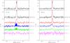 |
Fig. 1 Spectra of the observed transitions toward GO Tau and DM Tau. Intensity scale is |
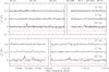 |
Fig. 2 N = 1−0 (top) and 2−1 (bottom) C2H emission toward CI Tau, CY Tau, and GO Tau. Conversion to flux density can be obtained by scaling by 6.1 Jy/K and 7.0 Jy/K the observed spectra, respectively. The red ticks indicate the expected positions and relative intensities of the hyperfine components. |
Integration times ranged from 1 to 2 h on source. Except for the CS(5−4) line where it reaches 20 mK, the median noise for all spectra is σT ≈ 13 mK at the δV ~ 0.25 km s-1 spectral resolution for most spectral lines, with relatively limited scatter (20%). The previous survey for 13CO, CN, and H2CO reached a similar sensitivity, although with a much larger scatter from source to source (7 to 25 mK) (Guilloteau et al. 2013). With a characteristic line width around ΔV ~ 3 km s-1, the flux sensitivity, 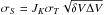 , is around 0.1 Jy km s-1. On average, our survey depth is 16 times better than those of Salter et al. (2011) and 3 times better than those of Öberg et al. (2010, 2011).
Figure 1 shows the spectra obtained for GO Tau and DM Tau, which illustrate the line shapes and the impact of the hyperfine structure for the C2H lines. Spectra for all sources are shown in Appendix B.
Fit results: HCO+ and HCN.
2.3. Ancillary 30 m data
In three sources, CI Tau, CY Tau, and GO Tau, we obtained high sensitivity spectra of the C2H N = 1−0 and N = 2−1 transitions. Each source was observed with the IRAM 30 m telescope in Jul. 2010 for about 6 h. We used wobbler switching, and the stable weather conditions yielded flat baselines. System temperatures were around 90−110 K at 3 mm, but ranged between 300 and 500 K at 174.7 GHz The spectra were smoothed to 0.26 km s-1 resolution, yielding a rms noise about 6 mK at 87 GHz for the 1−0 line, and 16 mK for the 2−1. Spectra are shown in Fig. 2. Lines are clearly detected in GO Tau. Summing the spectra of CI Tau and CY Tau (after appropriate recentering for their respective velocities) also indicates a 5σ detection in those sources (although each source is only detected at the 3σ level).
2.4. 30 m spectra analysis
All lines were fitted by simple Gaussian profiles. Although some of them are clearly double peaked (see Fig. 1), this process still gives the appropriate total line flux within the statistical uncertainties. Results are given in Tables 1−3. The N = 3−2 C2H transition is split into 11 hyperfine components, but 94% of the line flux comes in two well separated groups of two hyperfine components with a hyperfine splitting of about 3 km s-1, which is similar to the typical line width. We used the HFS method of the CLASS1 program to make a fit of all components together, assuming optically thin emission (total opacity <0.5). From the hyperfine line ratios, Punzi et al. (2015) find non-negligible optical depths for CN and especially C2H in LkCa 15. Their quoted values for opacities are within those allowed by our (somewhat less sensitive) data: our best-fit total opacity for C2H is 4, but with large errors (~2−3). DM Tau may also be partially optically thick in C2H with a total opacity of 0.8, but this value again has a large error. All other sources are consistent with optically thin emission. The reported flux in Table 3 is the sum of the four strongest transitions.
Fit results: CCH (main group of hyperfine components) and CS.
2.5. Interferometer data
To better constrain the disk properties, we use the CN and CO IRAM Plateau de Bure interferometer (PdBI) data reported in Guilloteau et al. (2014). In addition, we also analyzed in a similar way unpublished observations of GM Aur in CN, performed in compact configuration on 29 Oct, 2007, which yielded an angular resolution of 2.8 × 2.1′′. Figure 3 shows the resulting integrated spectra and integrated intensity maps of the two sets of hyperfine components.
Disk properties, specifically source velocity, disk inclination and outer radius, and star dynamical mass, are derived from these data sets, and completed by results from Simon et al. (2000), Piétu et al. (2007), Schaefer et al. (2009) when needed for higher accuracy. Similarly, the C2H PdBI data reported by Henning et al. (2010) for DM Tau, LkCa 15, and MWC 480 has been reanalyzed to provide a complementary view on the C2H distribution.
3. Results
HCO+ outer radii and line detections.
Combined with the previous study by Guilloteau et al. (2013), our survey provides an important quantitative step in the number of molecules detected in disks with 20 new detections of HCO+, 18 of HCN, 19 of CN, 11 of C2H, 10 of H2CO, 8 of CS, 4 of SO, and 4 of C17O in a sample of 30 disks, of which only 5 had already been studied extensively.
HCO+ is detected in practically all sources. Detection is marginal in two sources, CW Tau and LkHα 358, in which confusion with the molecular cloud makes the interpretation ambiguous (see Sects. 5.1 and 5.5). All strong lines are double peaked, as expected from Keplerian rotation in circumstellar disks. This also indicates that there is little contamination from the surrounding clouds (or outflows) for these sources. A few sources have very wide lines, in good agreement with the results from CN measurements of Guilloteau et al. (2013). A peculiar case is RW Aur, where the HCO+ line is extremely wide and may not originate from a circumstellar disk (see Sect. 5.9). HCN is detected in 20 (although marginally in CQ Tau and UZ Tau E) out of 30 sources. C2H is detected in 13 (ignoring AB Aur) out of 30 sources, and CS in 10 out of 29 sources (AB Aur was not observed in CS). Both lines are weak (peak flux 0.3−0.5 Jy).
Several lines of SO appear in the observed band, two of which are detected: the SO(65−54) line at 251.825816 GHz (in Haro 6-33 and IRAS 04302+2247, the Butterfly star, hereafter 04302+2247) and the SO(67−56) at 261.843756 GHz (in Haro 6-13, Haro 6-33, and 04302+2247, see Table 5). Combined spectra obtained by averaging the two lines are shown in Fig. 4. These spectra also suggest a marginal detection in GM Aur.
No other molecule is detected in the band, which included lines of HOC+, two lines of HC3N and the H13CO+J = 3−2 transition. The latter provides upper limits to the HCO+ opacity (see Sect. 4.3 for details).
4. Analysis method
4.1. Definition of disk radii
In the following sections, we introduce several radii with the goal of characterizing the size of the observed disks in a consistent way. In Sect. 4.2, we first use a simple approximation to derive the outer radius of the molecular distribution of HCO+, R(HCO+), using the same approach as Guilloteau et al. (2013) for CN. In Sect. 4.4, we also show that an estimate of the outer radius can be obtained from the overall shape of the line profile, when the stellar mass is known. Finally, Sect. 4.5 derives radii based on a detailed modeling of the line emission, using a three-dimensional (3D) ray tracing code to simulate the emission from a disk with a power distribution of molecules and temperatures. The derived outer radius of that distribution is called Rsingle if only the line profile can be fit, and Rinter when we can model resolved images of the line emission. Based on these independent estimates, we show that a single radius is sufficient to characterize the HCO+ and CN emission, and that of C2H, when the later method can be applied to it. This disk radius Rdisk is then used to derive the molecular column densities from the optically thinner emission of other molecules.
Although real molecular distributions are not truncated power laws, this model can still be a reasonable approximation. This happens because the density in disks is falling rapidly with radius, for example, as 1 /r3 for a surface density falling as 1 /r1.5 and an isothermal disk, and even more steeply for exponentially tapered profiles predicted by viscous evolution models. This implies a sharp transition beyond which the observed spectral lines become unexcited. Only CO, because of its low critical density, may behave differently and have a larger outer radius.
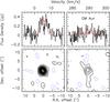 |
Fig. 3 Integrated spectra of the two groups of hyperfine components for CN N = 2−1 line, and maps of the S/N toward GM Aur (contours are in steps of 2σ). The profile of the best-fit disk model (see Sect. 4.5) is shown in red. |
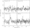 |
Fig. 4 Averages of the SO(65−54) and SO(67−56) spectra resampled to a common velocity scale. |
4.2. Radii from line flux
Line formation in a Keplerian disk is largely dominated by the Keplerian shear (Horne & Marsh 1986). We use the approach described in Guilloteau et al. (2013, Appendix D), to which we refer for additional details. The integrated line flux is given by  (1)for inclinations i< 60−70°. The value T0 is the average disk temperature, ΔV the local line width, Rout the disk outer radius, and D the source distance. The parameter ρ is a dimensionless factor that depends on the line opacity τl (see Guilloteau & Dutrey 1998, their Fig. 4), and ρ ≈ τl, for optically thin lines, saturating as ∝ log (τl) for large optical depths. In the optically thin regime, τl is inversely proportional to cos(i) and ΔV and proportional to the molecular column density, so the dependency on inclination and line width cancels, and the flux just scales with the total number of molecules. For optically thick, nearly edge-on objects, where the above formula breaks down, Beckwith & Sargent (1993) have shown that the expected flux is not a strong function of inclination, so using cosi = 0.5 remains appropriate. Inverting Eq. (1), the outer radius is given by
  (2)In disks, the local line width is typically around 0.2 km s-1 (e.g., Piétu et al. 2007), so the outer radius can be derived provided ρ and T0 can be estimated. In Guilloteau et al. (2013), we used the hyperfine structure of CN to provide an estimate of the line opacity, and thus of ρ, and simply assumed T0 = 15 K for large disks around T Tauri stars, and 30 K for small disks, or those around HAe stars. We show in the next paragraph that using ρ = 1 is appropriate for HCO+.
SO detections.
4.3. HCO+ line flux
Simple approximation: ρ(HCO+) = 1
Some upper limit on the HCO+J = 3−2 line opacity comes from the nondetection, or at best marginal detection, of the H13CO+J = 3−2 transition. For the strongest HCO+J = 3−2 emitter, 04302+2414, H13CO+J = 3−2 is at least 20 times fainter. Combining the signals from the stronger sources (recentered on the source velocity and weighted by the HCO+J = 3−2 detected line intensity, but not rescaled in terms of line width), we obtain a marginal detection of H13CO+J = 3−2 at a level 20 times lower than that of the main isotopologues. Therefore, the average opacity of the HCO+J = 3−2 line does not exceed a few. We thus use ρ = 1 in Eq. (2). As in Guilloteau et al. (2013), we also assume ΔV = 0.2 km s-1, and T0 = 15 (for T Tauri stars) or 30 K (for F and A stars, or small disks; see Table 4 Col. 3 for the value used for each source).
The derived outer radii, called R(HCO+), are given in Table 4, and are in general very consistent with prior knowledge coming from resolved images made with interferometers (see Table 4 Col. 10 and associated references) despite our very crude assumption about the disk temperature and HCO+ opacity. For 17 sources, the radii match to better than 20%, while for the 10 remaining sources, R(HCO+) is larger (3 sources have no other reliable radius).
If the HCO+(3−2) line was optically thin, lower values of ρ should be used, which would imply larger disk radii, becoming inconsistent with the CN radii, and even exceeding the radii derived from CO. This simple exercise shows that the HCO+J = 3−2 transition is mostly optically thick in all disks. As a consequence, it implies that the HCO+ content cannot be simply determined from this transition (which only sets a lower limit), and that direct comparison of intensity ratios between HCO+(3−2) and other transitions are meaningless. A more complete disk model, as done in Sect. 4.5 is required for HCO+. On the contrary, all other transitions in general have significantly lower flux2, and thus must be optically thin. For C2H, one should consider the line flux per hyperfine component, which is only 0.3 times the integrated line flux given in Table 2. The same remark also applies to CN lines.
Interferometric modeling of CN N = 2−1.
Discrepant radii: warmer and/or younger sources?
Where a difference exists, the HCO+-based radius is larger than the interferometric measurement. Measurements based on CN only give a lower limit to the disk radius because the CN N = 2−1 line may be subthermally excited in the outer disk, while HCO+ is more easily thermalized. In some cases, however, the HCO+-based radius is larger than the radius measured in CO. To reconcile both values, we can thus either (1) increase ρΔV or (2) increase the temperature T0 in Eq. (2). The parameter Rout would only scale as 1 / log (τ) in case (1), so the required increase in τ might conflict with the upper limit on H13CO+. Thus case (2), where Rout scales as 1/ , is more likely. In fact, such differences are most prominent on smaller disks, which are probably on average warmer than larger sources, as the temperature drops with radius roughly as r− q with q ≈ 0.5−0.6 in disks. This could apply to DL Tau and CY Tau, which would need to be a factor 2 warmer to reconcile radii. It is also possible that the local line width ΔV is larger in smaller disks.
In all cases, this is insufficient for Haro 6-33, where we already assumed a relatively warm disk, or Haro 6-13, where a factor 4 in temperature would be needed. We note in this respect that both sources are heavily confused, so it is possible that the CO radius derived by Schaefer et al. (2009) is biased toward low values because one cannot get the full disk extent near the systemic velocity.
It is also worth noting that Haro 6-33 has the strongest CS/CN line ratio compared to any other source, reflecting perhaps an unusual chemistry. Its relatively high content of S-bearing molecules is also attested by the detection of SO lines. Contamination by an outflow is not fully excluded.
4.4. Radii from line profiles
In any case, the radii given in Table 4 are only very simple estimates. Another approach consists in deriving the outer radii from the separation of the two velocity peaks in the line profile, ΔVpeak. Because of the Keplerian velocity field, this separation is  (3)so if the stellar mass M∗ and disk inclination i are reasonably well known, the outer radius can be estimated. Instead of using Eq. (3) directly, in the next section we develop an analysis based on a complete disk modeling to simulate the line profiles. This is possible for sources for which sufficient interferometric data (or other ancillary information) allow us to constrain the basic disk geometry, as detailed below.
Modeled column densities from the 30 m data.
4.5. From flux densities to molecular column densities
When the basic disk geometry, source velocity, disk inclination and star dynamical mass, is known, a simple power-law disk model can allow us to retrieve other disk parameters, such as the (excitation) temperature radial profile (for mostly optically thick lines) or the molecular surface density radial profile (for optically thin lines). The assumed profiles are
 for the molecular surface density and (rotation) temperature, respectively. The choice of the pivot, 300 and 100 au, is made to minimize the errors on the values at this radius, as discussed in Piétu et al. (2007).
Even in case of low S/N, useful limits on molecular column densities can be obtained by assuming, for example, that the (excitation/rotation) temperature of the molecule is given from other measurements, that is, either CO or HCO+ transitions. Some assumptions about the local line width are required, but it only matters for substantially optically thick lines.
We use the DiskFit tool (Piétu et al. 2007) to adjust the observed line profiles, following the method used by Dutrey et al. (2011) for the study of S-bearing molecules. DiskFit minimizes a χ2 function in the uv plane, comparing the measured visibilities (or line flux in case of single-dish profiles) to those predicted by the ray tracing code. Each visibility is weighted according to the theoretical noise derived from system temperature, channel width, and integration time. The minimizations are performed using a modified Levenberg-Marquardt and the errors derived from the covariance matrix.
We assume the exponent of the temperature profile is q = 0.4. The local line width is set to 0.16 or 0.2 km s-1; HK Tau required a higher value to best fit the profiles, but this local line width has no impact on the derived column densities. In a first step, to determine the systemic properties (LSR velocity, inclination i, and stellar mass M∗), we used the interferometric data, leaving p, the temperature T, and the outer radius Rout as free parameters. Results obtained from CN are given in Table 6.
The derived values of i,T,M∗, and Rout were used for single-dish analysis, for which we fix p = 1. The exponent p has little impact on the column densities at 300 au. p = 1 is within the errors of the values found from the interferometer data: the weighted mean of the values in Table 6 is 1.15 ± 0.16. The temperature value T also has limited influence because the 2−1 and 3−2 transitions of the observed molecules are mostly sensitive to the column density because of the compensation between excitation temperature and partition function for temperatures between 10 and 25 K (see, e.g., Dartois et al. 2003, their Fig. 4). A possible exception is the CS J = 5−4 line, which becomes sensitive to the temperature below 15−20 K. In this respect, the small (factor 2) difference between the column densities given for DM Tau by Dutrey et al. (2011) from the J = 3−2 line and those found here could be due to a somewhat higher (rotation) temperature than assumed.
The single-dish spectra are then constrained by a single free parameter: the molecular column density at 300 au, Σ. When no CN interferometric data is available, the temperature is taken from CO interferometric data if possible (which may overestimate the actual rotation temperature of most molecules because of the vertical temperature gradients in disks), or simply assumed. For disks without CN interferometric data, Rout is also adjusted to best fit the HCO+ spectrum.
The sources that are well suited for this study are CY Tau, HV Tau C, IQ Tau, DL Tau, DM Tau, GG Tau, UZ Tau, CI Tau, DN Tau, LkCa 15, GO Tau, GM Aur, MWC 480, and the Butterfly star, 04302+2247. Haro 6-13 and Haro 6-33 can be studied with less precision because of the limited accuracy on their disk parameters from the CO data of Schaefer et al. (2009). Similar caution should be applied to AB Aur because of the source complexity (Piétu et al. 2005). The small disk sizes of CQ Tau and MWC 758 also result in limited accuracy.
Despite a lack of accurate sizes from interferometric data, we also consider RY Tau, HK Tau, AA Tau, Haro 6-5b, and DO Tau because all have sufficiently well constrained inclinations to allow some estimate of disk sizes from the HCO+ spectra. We assumed a stellar mass of 2.2 M⊙ for RY Tau and a systemic velocity of 6.75 km s-1. For HK Tau, we assume all the emission is coming from HK Tau B because it is the most massive and most inclined disk of the system, and thus better fits the wide lines that are detected.
We exclude CW Tau, HH 30, and LkHα 358 from the analysis because of contamination by the cloud, and we also exclude SU Aur and RW Aur because of their peculiar nature and very small disks. Little can be said for very small disks (≤150 au), as only substantially optically thick lines are detectable in this case.
The fitted lines include HCO+(3−2), HCN(3−2), CN(2−1), C2H(3−2), CS(5−4), plus the SO and (ortho)-H2CO lines when detected. We do not consider 13CO(2−1) for two reasons. First, for many sources, the IRAM 30 m telescope spectra are affected by strong contamination from the surrounding molecular cloud. Second, when interferometric data are available (DM Tau, LkCa 15, and MWC 480, Piétu et al. 2007; GM Aur, Dutrey et al. 2011), the exponent of the surface density law, p, is often much steeper (p> 2−3) than for CN or HCO+. This steep exponent probably reflects only the very outer parts of the disks, where the 13CO lines are optically thin, but transitions from other molecules are no longer excited.
Results for column densities are given in Table 7 and ratios in Table 9.
4.6. C2H multitransition analysis
For C2H, three sources have been previously imaged with the IRAM PdBI array in the N = 1−0 and 2−1 lines at ~3′′ resolution: DM Tau, LkCa 15, and MWC 480 by Henning et al. (2010). For DM Tau and LkCa 15, our column densities derived from the N = 3−2 lines under the simple hypothesis above are a factor 2 larger than those of Henning et al. (2010). This probably reflects a somewhat higher excitation temperature than assumed. The results, provided by DiskFit as described in Sect. 4.5, using this data combined with the N = 3−2 spectra are given in Table 8, assuming q = 0.4. The derived temperatures, 15 and 16 K, are indeed slightly above those quoted by Henning et al. (2010), 11 and 10 K for DM Tau and LkCa 15, respectively. In MWC 480, the interferometric data has a low S/N and thus a limited influence on the global fit.
In addition, the N = 1−0 and 2−1 transitions of C2H were observed at the IRAM 30 m telescope for CI Tau, CY Tau, and GO Tau. Lines in GO Tau are well detected, but those in CI Tau and CY Tau were only marginally detected. These spectra were used in a multiline fit to derive the C2H column density in these three sources, with results given in Table 8. Overall, the fit results are in remarkable agreement with those of the CN interferometer data in terms of disk radii but also excitation temperatures. The excitation temperatures derived from CN or C2H also agree with the values assumed for HCO+. This gives credit to our simple assumption for temperatures, and thus to the disk radii derived solely from HCO+ in other sources.
We note that excitation temperatures and column densities for C2H in LkCa15 found in this detailed disk modeling are quite different from those derived by Punzi et al. (2015) from the N = 3−2 IRAM 30 m telescope spectra alone. This is presumably because Punzi et al. (2015) assumed a uniform beam filling factor in the 30 m telescope beam, of order 1 given the outer radius of the disk, ~500 au, and thus derive very low excitation temperatures (as the opacity of each of the detected hyperfine component is ~0.5 from the hyperfine ratios). Consequently, these underestimated temperatures result in high column densities because of the partition function at very low temperatures.
However, in a Keplerian disk, the filling factor is limited to less than ~δv/Vkep(Rout) by the Keplerian shear, and is affected by the cos(i) factor due to the inclination (e.g., Horne & Marsh 1986; Guilloteau et al. 2013, their Appendix D). In the case of LkCa 15, this filling factor is at most ~0.05. The full multiline disk modeling explicitly accounts for the details of the line formation mechanism and provides reliable estimate of the column density and excitation (although of course under the power-law approximation).
Multitransition modeling of C2H.
Column density ratios at 300 au.
5. Individual sources
This section summarizes specific information required for several sources to interpret the results of Tables 1−3 and the detailed analysis presented in Sect. 4.5. It also provides new information on previously unknown or poorly characterized gas disks.
5.1. CW Tau
From the 13CO PdBI data of Piétu et al. (2014), the systemic velocity is 6.45 km s-1 and the best fit model leads to an integrated line flux of 2 Jy km s-1. These values are consistent with those derived from the IRAM 30 m telescope measurements of Guilloteau et al. (2013), who showed that contamination by the molecular cloud appears in CN and H2CO at a systemic velocity of 6.80 km s-1. Here, the HCO+(3−2) spectrum is consistent with the redshifted part that is obscured by the molecular cloud, leaving only the blueshifted wing detected at the 4σ level.
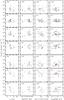 |
Fig. 5 Correlation plot of the column density of molecules at 300 au with stellar luminosity, spectral type, 1.3 mm flux density and stellar age. Embedded objects appear in red, HAe stars in blue, and T Tauri stars in black. Error bars are ± 1σ with limits at 2σ indicated by arrows. |
5.2. DO Tau
The properties of DO Tau are poorly known. Koerner & Sargent (1995) detected CO emission, but with a very broad blueshifted wing, which probably traces an outflow, and may indicate that this source is quite young. Indeed, it is surrounded by an optical nebulosity along a redshifted optical jet (see Itoh et al. 2008, and references therein). Kwon et al. (2015) obtained a measurement of the disk inclination i = 32 ± 2° through high resolution imaging with CARMA. The stellar mass is not known; we assumed M∗ = 0.7 M⊙ in our analysis. The HCO+ and CN line profiles are then consistent with an outer disk radius of 350 au and a systemic velocity of 6.5 km s-1. The CS data indicate a possible ~5σ detection, but the derived velocity, ~4.3 km s-1, does not agree with the better determination from HCO+ or CN, so we consider this as noise.
5.3. RY Tau
The HCO+ detection is convincing (6σ level), but the line is very broad. The centroid velocity and line width are consistent with the tentative detection of CN by Guilloteau et al. (2013). Assuming similar line parameters, the HCN detection is marginal (4σ). CS is not detected. CO observations at the IRAM interferometer (Coffey et al. 2015) indicate a LSR velocity of 6.75 km s-1, and the system is highly inclined (70°). The large line width is consistent with a 2 M⊙ star indicated by the spectral type F8, provided the disk is not too large (<300 au).
5.4. Haro 6-5 B
This nearly edge-on object is very young and still embedded in a substantial envelope. The HCO+ line width is somewhat larger than the CN line width, which may indicate that part of the HCO+ emission comes from an outflow, as Haro 6-5 B drives a powerful optical jet (Liu et al. 2012). Yokogawa et al. (2002) suggested that Haro 6-5 B is a very low-mass object, 0.25 M⊙, based on 5′′ resolution images of 13CO, but our HCO+ spectrum, if arising from a disk only, indicates this is a 1 M⊙ star.
5.5. LkHα 358
There is a tentative HCO+ detection of a very narrow line, which is not compatible with the compact CO disk detected by Schaefer et al. (2009). There is strong confusion in CO isotopologues (including C17O) toward this line of sight. The HCO+ profiles however match the 13CO profile obtained by Guilloteau et al. (2013). 13CO and HCO+ lines may originate from a disk, with the inner parts of the spectra hidden by strong confusion due to the Taurus cloud. LkHα 358 is located deep in the this cloud, near HL Tau and HH 30. It is also possible that these lines originate entirely from the cloud. The detection of C17O at a LSR velocity of 7.05 km s-1 (very close to the disk systemic velocity, 6.8 km s-1) and with a line width of 0.45 km s-1 indicates a high column density, and the positive signal in 13CO and HCO+ may just be the wings of the cloud emission profile.
Figure 6 shows the relevant spectra. It shows that the tentative fit of a disk component in 13CO by Guilloteau et al. (2013) most likely overestimated the disk contribution. A similar fit to the HCO+ profile (masking the same velocity range for both lines, 6.0 to 7.5 km s-1) yields an integrated line flux of 0.15 Jy km s-1 with a 5σ significance. Assuming the same excitation temperature as for CO (25 K as measured by Schaefer et al. 2009), such a flux would be compatible with optically thick HCO+ emission out to 130 au, which is consistent with the disk size in CO. LkHα 358, one of the lowest mass stars in our sample, has a mass of 0.33 ± 0.04 M⊙, using the inclination of i = 52 ± 2° found by ALMA Partnership et al. (2015) and the vsin(i) = 1.35 ± 0.04 km s-1 from Schaefer et al. (2009).
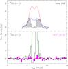 |
Fig. 6 Spectra of 12CO, 13CO, and HCO+ toward LkHα 358. Top: 12CO from the interferometric measurement of Schaefer et al. (2009). The blue curve is the fitted profile based on the disk analysis made in the uv plane. The red curve uses the same disk parameters, except for the outer radius which is 250 au instead of 170 au. Bottom: 13CO(2−1) spectrum (histogram) and HCO+(3−2) (filled histogram). The green curve is the tentative fit of a disk component from Guilloteau et al. (2013). |
5.6. GG Tau
GG Tau is a hierarchical quintuple system (Di Folco et al. 2014). The disk is around the central triple star. Molecules in GG Tau were already detected by Dutrey et al. (1997). We obtain here better S/N and detect C2H for the first time. For the disk analysis, we assume an inner radius of 180 au to account for the large cavity sculpted by the tidal interactions with the binary (Dutrey et al. 2014a), as only 12CO has been detected from within the cavity so far.
5.7. AA Tau
Emission from the disk of AA Tau is known to be affected by contamination due to the molecular cloud, especially in CN (Guilloteau et al. 2013). Contamination may also affect the HCO+ spectrum, which displays a similar velocity as CN, but is different from those of HCN, 13CO, and C2H. CS is also apparently detected. In the analysis, we also used the integrated profiles obtained with the SMA by Öberg et al. (2010) for CN, HCN, and HCO+ to improve the sensitivity in the fit.
5.8. SU Aur
The origin of the HCO+ emission is unclear. The (partially confused) emission detected in 13CO by Guilloteau et al. (2013) with the IRAM 30 m telescope closely agrees with the interferometric result of Piétu et al. (2014). The HCO+ spectrum displays in addition to this disk component a prominent blueshifted wing, which may be the trace of an outflow. No other molecule is detected.
5.9. RW Aur
RW Aur is a binary system that was imaged in 12CO by Cabrit et al. (2006), who find evidence for a very small (50 au radius) disk, but did not detect 13CO emission. The rather strong, but very broad, HCO+ line may come from the tidal arm detected in CO by Cabrit et al. (2006), rather than from a very compact disk. An origin in a disk would imply very hot gas, and a very massive system.
5.10. HK Tau
HK Tau is a binary system and it is possible that the line emission originates in part from both stars, as they have similar disks in CO (Jensen & Akeson 2014). However, the HCO+ line width is quite large, and given the estimated stellar masses of 0.6 and 1.0 M⊙ for A and B, respectively (Jensen & Akeson 2014), we tentatively assign the origin of the emission to the edge-on disk HK Tau B. The large line width then implies an origin in a rather compact disk, of characteristic outer radius 100 au, and a substantial optical depth is required to provide enough flux implying ρ ≈ a few in Eq. (2). The modeling of the line profile indeed requires a small, warm disk with higher local line width than in other sources, however, contamination by the disk of HK Tau A may also partly explain the relatively high flux of the HCO+(3−2) line.
5.11. FT Tau
CO detection of FT Tau was reported by Guilloteau et al. (2011), who found a disk inclination around 30°, but with large uncertainty despite the high angular resolution (0.5 × 0.3′′) because the disk is small, both in line and continuum, and the CO emission is severely contaminated by a molecular cloud between 5 and ≈8 km s-1. Although Garufi et al. (2014) argue for higher inclination, based on unresolved spectral energy distribution and line emission modeling, a recent measurement of the dust disk inclination using CARMA gave i = 34 ± 2° (Kwon et al. 2015). The detection of several transitions (HCO+, CN, and marginally C2H) indicates a systemic velocity of 7.3−7.4 km s-1, confirming that the blueshifted part of the disk is hidden by the cloud in CO. To best fit all available lines, we need a small disk, orbiting a M∗ = 0.35 M⊙ for i = 34°. Higher inclinations would require an even less massive star (as vsin(i) must be preserved) and are thus unlikely. The disk radius must be around 200 au: larger disks produce too much flux. Figure 7 shows the fitted profiles for CO and HCO+ and the CO-integrated area map using data from Guilloteau et al. (2011). The small disk size makes FT Tau similar to the “mm-faint”, compact disks studied by Piétu et al. (2014). The detection of molecules there thus indicates that the chemistry on scales 100−200 au is not widely different from what happens in bigger disks at radii 200−500 au.
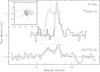 |
Fig. 7 Observed spectra and fitted profiles for FT Tau. The gray area is the range affected by confusion from the molecular cloud that is ignored in the CO analysis. The insert shows the integrated CO emission with contour spacings of 50 mJy km s-1 (angular offsets in arcsec). The cross indicates the position and orientation of the disk (derived from the continuum emission and kinematics pattern). |
6. Discussion
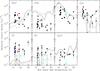 |
Fig. 8 Predicted column densities at 300 au as a function of disk midplane temperature with observed points superimposed. Color markers are DM Tau (red), GO Tau (blue), and MWC 480 (cyan). The continuous line is for “standard low metal” abundances, while the dashed line assumes an additional depletion of C and O by a factor 10. |
6.1. Molecular sample
A comparison with the unbiased frequency survey of Punzi et al. (2015) shows that, although covering only half of the 64 GHz between 206 and 270 GHz, our study only misses three detectable transitions: 12CO J = 2−1, which would be severely contaminated by molecular cloud emission in most cases, C18O J = 2−1, and the 30,3−20,2 transition of para H2CO at 218.222 GHz. The only other significant molecules missed by both studies, because of their upper frequency cutoff of 270 GHz, are HNC and N2H+, whose 3−2 rotational lines are at 271.981 GHz and around 279.5 GHz respectively.
Less abundant molecules, such as the deuterated species DCO+ and DCN, or the more complex molecules, such as HC3N, C3H2, fall in our observed band, but require much deeper integration to be detectable.
We have for the first time discovered several molecules in several disks of radii <250 au (RY Tau, FT Tau, IQ Tau, DN Tau, UZ Tau E, and HK Tau). This demonstrates that the TW Hya disk is not specific in this respect, and shows that the chemistry of these regions is not fundamentally different from that of much larger disks like DM Tau or GO Tau.
Our data includes stars with spectral types from M3 to A0, stellar masses from 0.3 to 2.2 M⊙, luminosities from 0.1 to 40 L⊙, and ages ranging from <0.5 to more than 4 Myr. A summary of star and disk properties is given in Table A.1. The column densities of the detected molecules are shown as a function of stellar ages, luminosities, and spectral type, and also 1.3 mm continuum flux in Fig. 5. The 1.3 mm flux is often used as a possible proxy for the disk masses, but temperature and opacity effects both play a non-negligible role in the derivation of masses from continuum flux, as discussed in Appendix A. Although disk masses span the range from 0.003 to 0.1 M⊙, they cluster around 0.015−0.020 M⊙.
Only two main trends are visible in Fig. 5: a general decrease of molecular column densities as a function of stellar luminosity (except for H2CO) and an overall increase in CN, C2H, and HCN as a function of stellar ages. These two trends may provide a natural explanation for the lower CN emission found by Reboussin et al. (2015) in disks in the younger association ρ Oph, as stars are (on average) both younger and more luminous there than in the Taurus region. The statistical significance of this trend remains low and the dispersion quite high. A log-log correlation analysis of N(HCO+) versus L∗ yields a correlation coefficient of r = −0.48 (p value of 0.02). A Spearman test gives a similar result (r = −0.505 and p = 0.014) and all other correlations are less significant.
On the other hand, a statistical analysis reveals substantial correlations between HCO+, CN, C2H, and HCN surface densities. The strongest correlations are for CN with HCN, and CN with C2H. We find a log-log correlation coefficient of r = 0.84 (Rank-Spearman p = 7 × 10⁻⁷) between the column densities of CN and C2H, similar to that for CN and HCN (r = 0.86,p = 2 × 10⁻⁷). Correlation between these molecules and HCO+ come next with r between 0.56 and 0.70. Line ratios may thus be better diagnostic tools than line intensities. These ratios are given in Table 9 and are shown as a function of disk/star properties in Figs. A.1 and A.2. Although ratios vary by a factor >10 from source to source, no obvious correlation emerges from this analysis. For T Tauri stars, the [CN/HCN] and [C2H/HCN] ratios are higher than in typical molecular clouds (e.g., for TMC-1 (CP) Ohishi et al. 1992), confirming the results found previously for other sources (Dutrey et al. 1997; Kastner et al. 2014). This is suggestive of photodissociation processes, for which we would expect CN and C2H to be correlated as in our data. The [CN/C2H] ratio still varies substantially from source to source, however, possibly indicating other chemical processes at work.
We also caution that despite the substantially larger number of sources compared to previous studies, each category still only contains a few sources. For example, the only “warm” disk that is well probed by our data, MWC 480, is a heavily self-shadowed disk with little flaring, whose properties are very close to those of T Tauri disks. AB Aur is still embedded in an envelope (Tang et al. 2012), and has a large (100 au radius) inner cavity (Piétu et al. 2005), so may be atypical. The warmer disks around Group I (Meeus et al. 2001) HAe stars, such as CQ Tau and MWC 758, are unfortunately too small for precise measurements. Nevertheless, these two stars are among those with the lowest column densities of HCO+, CN, HCN, and C2H, but are strong in CO isotopologues. In fact, the molecule-to-CO ratio is smaller in MWC 480 than in any T Tauri disk. A high CO content for MWC 480 (as well as for AB Aur and 04302+2247) is attested by the detection of C17O J = 2−1 transition, which is below our detection threshold for all T Tauri disks (Guilloteau et al. 2013). A comparison with the other small disks also indicates that HCO+ and CN are substantially less abundant in CQ Tau and MWC 758 than in the T Tauri stars. This confirms the overall deficiency in molecules in HAe disks found in the case of AB Aur by Schreyer et al. (2008), which they explain as a result of enhanced photodissociation due to the large UV flux from the host star. We note that such an enhancement is not included in Fig. 8.
Another noticeable trend is more S-bearing molecules and less CN in the embedded, presumably younger objects like Haro 6-10, 6-33, 6-5B, DO Tau, and the Butterfly star. These young sources also have more H2CO than more evolved T Tauri disks. A higher H2CO content is also found in warm disks around Herbig Ae stars, as indicated by AB Aur and (tentatively) CQ Tau.
6.2. Comparison with chemical modeling
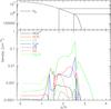 |
Fig. 9 Predicted molecular densities at 300 au as a function of height above the disk midplane (in scale heights, defined as cs/ Ω, where cs is the sound speed, and Ω the Keplerian angular frequency). The upper panel shows the H2 density with the two horizontal and vertical lines delimiting the range where most molecules are abundant. |
A full chemical modeling of the observed disks is beyond the scope of this work. We however show some results using the disk chemical model described in Reboussin et al. (2015). We use here a density distribution with a p = 1 exponent for the surface density and a disk mass of 0.03 M⊙ for a disk extending up to 800 au; these are roughly the expected disk parameters for DM Tau and GO Tau. The thermal structure is not derived self-consistently. Instead, the midplane temperature is taken as a free parameter, and a vertical gradient is included with temperatures at 2 scale heights that are typically higher than in the midplane by 10 K. The density profile is derived from hydrostatic equilibrium. The UV flux impinging on the disk is representative of T Tauri stars.
The model solves the time-dependent chemistry at each radius independently, using a complex gas + grain chemical network, involving reactions on dust grains. The grain size distribution is equivalent to 0.1 μm grains. Photodesorption was shown by Reboussin et al. (2015) to be negligible in these conditions and is thus not included. The disk age is assumed to be 1 Myr. Column densities of several molecules as a function of the disk midplane temperature are shown in Fig. 8. We have overplotted the observed points, assuming the apparent excitation temperature of the observed transitions is representative of the midplane kinetic temperature (see justification below). The model roughly reproduces the observed surface densities of CN and C2H for disk midplane temperatures below 15 K, which is consistent with the fitted temperatures derived from the CN interferometric data. The CN/HCN ratio also agrees with the measured ranges for cold disks.
The simple combination of surface reactions (leading to more complex molecules on grains) and thermal and nonthermal desorption mechanisms are sufficient to produce C2H and CN. CN and C2H, as well as all other molecules, are approximately colocated at around 2 scale heights (density seven times below the disk plane density) above the disk (Fig. 9). At 300 au, the density in this region is in the range 1−4 × 106 cm-3, providing enough collisional excitation for the observed transitions, but not a complete thermalization. We thus expect Tex ~ 0.7 Tk(z = 2H) for most transitions, except perhaps for HCN(3−2) which has the highest critical density of all observed molecules. This region is slightly warmer than the disk midplane, however, so both differences compensate to first order, and Tex is close to the midplane temperature Tk(z = 0).
The model does not include X-ray ionization, so predictions for HCO+ should be considered with more caution. Henning et al. (2010) also showed that C2H could be produced in substantial quantity close to the disk plane in presence of X-ray ionization at radii <100 au, but our observations are not sensitive to these small radii. In our chemical model, C2H behaves differently at 100 au than at 300 au, perhaps explaining why the CN/C2H ratio varies from source to source.
HCN is overpredicted by the chemical model by a factor of ~5 on average. However, part of this may be an artefact of our assumed excitation temperature for this line, because HCN J = 3−2 is the transition with the highest critical density, and thus the most susceptible to subthermal excitation. Indeed, based on resolved observations of the HCN J = 1−0 line, which is largely optically thin as attested by the hyperfine component relative intensities, Chapillon et al. (2012b) found column densities of 7 and 11 × 1012 cm-2 for DM Tau and LkCa 15, respectively, which is a factor 2 and 1.5 above our derived values. Non-LTE effects may become relatively more important in lower mass disks.
Finally, as in most other chemical models, the S-bearing molecules are not well reproduced: CS is underpredicted and SO overpredicted. Dutrey et al. (2011) showed that in particular H2S is not detected in disks, which suggests that current chemical models lack a major process of chemical evolution of S bearing molecules on grains.
Recent works comparing the observed OI, CI, C+, and high J CO line intensities to predictions of thermochemical models (Chapillon et al. 2010; Bruderer et al. 2012; Du et al. 2015) suggest that C and O are depleted in the upper layers of the disk. A possible mechanism to obtain such an elemental depletion resides in the disk history coupled to the dust grain evolution in the cold midplane layers of the disk. Carbon and oxygen nuclei get trapped in the form of CO or CO2 on grains around the midplane, as shown by Reboussin et al. (2015). Simultaneously, as turbulent mixing drags the gas and smaller grains up and down, the upper layers can progressively be depleted in C and O nuclei in the gas phase. Grain growth in the disk midplane could potentially accelerate this overall gas phase depletion. We computed a second set of chemical models simply assuming C and O are depleted by a factor 10. The results are shown as the dashed lines in Fig. 8. We note a decrease in C2H surface densities. HCN and CN are less affected by this important reduction of the number of available C nuclei, but the predictions remain in broad agreement with the observations (CS excluded as before). Another interesting effect is the substantial reduction of SO, which practically scales as the O depletion factor. A progressive reduction in elemental abundances in the gas phase with time would thus naturally lead to stronger SO emission in younger objects, which perhaps explains why SO is only detected in embedded sources. Semenov & Wiebe (2011), however, found SO to be sensitive to turbulent transport in the disk.
7. Conclusions
We have performed a (spatially unresolved) survey of 30 disks in the Taurus region with the IRAM 30 m telescope with sufficient sensitivity to detect HCO+, CN, HCN, C2H, H2CO, CS, SO, and C17O, allowing us over 100 new detections of individual spectral lines from these 8 molecules. The detection rates range from ~100% (for HCO+) down to <15% (for SO and C17O). Our results are as follows:
-
A comparison with Punziet al. (2015) on LkCa 15, one of thetwo strongest sources in our survey, shows that, except for C18O andone para H2CO line, our study covers all lines detectable in the206−270 GHz range with integration times of~2−8 h per source using a telescope as sensitive as theIRAM 30 m.
-
The HCO+ line flux is consistent with moderately optically thick emission extending out to radii comparable to the outer radius derived from CN or CO interferometric observations, which thus define “the disk radius”. All other lines have lower opacities.
-
The survey is complemented by resolved observations of CN (or CO) in many sources, and with (resolved or unresolved) multiline observations of C2H in six sources, allowing an estimate of disk radii and excitation conditions. The typical excitation temperatures derived for CN and C2H range from 8−10 K at 300 au to 15 to 30 K at 100 au.
-
The overall consistency between HCO+, CN, and C2H suggests that non-LTE effects are limited for these molecules, although it is still possible to have Tex ≈ 0.7Tk for most observed transitions. In particular, we do not confirm the very low excitation temperatures suggested for CN and C2H in LkCa15 by Punzi et al. (2015); consequently, we do not confirm the very high column densities for these two molecules.
-
Practically all T Tauri stars share very similar characteristics with enhanced CN/HCN and C2H/CN ratios compared to molecular clouds. The detection of several molecules in small disks (radii ~200 au) indicates the chemistry in these regions is not radically different from that of bigger disks, as already hinted at by the only known detailed case so far, TW Hya (Thi et al. 2004; Kastner et al. 2014).
-
As suggested by the previous study of AB Aur (Schreyer et al. 2008), disks around HAe stars appear less rich in molecules. Unfortunately two of the five studied disks around HAe stars are small, and the current sensitivity level is insufficient to be quantitative on the abundance of molecules. More generally, the number of molecules appear to decrease with stellar luminosity.
-
The content in CN and C2H seems to increase with stellar age, a result corroborating the lower CN line flux found by Reboussin et al. (2015) in the younger ρ Oph association.
-
We performed a simple chemical modeling showing that gas-grain chemistry predicts molecular column densities in reasonable agreement with the observations with the noticeable, but well known exception of S-bearing molecules.
-
Progressive depletion of C and O, due to buildup of CO and CO2 ices on dust grains and turbulent mixing may be a clue to explain the higher SO content of young disks.
These observations pushed the IRAM 30 m telescope to its ultimate capabilities for sensitive spectral line surveys of many (unresolved) sources. Disks that are smaller than about 150 au are no longer detectable in reasonable integration times. The success of our strategy however yields promise for interferometric surveys. For example, NOEMA will be able to provide the same frequency coverage in just two setups and would be sensitive enough to go a factor 4 to 6 times deeper in the same integration time. The spectral capabilities of the even more sensitive ALMA array are less flexible, but still allow several combinations of three reasonably strong lines from the above molecules to be covered simultaneously in band 6 or 7.
Except for HCN in LkCa 15 and perhaps DN Tau.
Acknowledgments
This work was supported by “Programme National de Physique Stellaire” (PNPS) and “Programme National de Physique Chimie du Milieu Interstellaire” (PCMI) from INSU/CNRS. WV’s research is funded by an ERC starting grant (3DICE, grant agreement 336474). D.S. acknowledges support by the Deutsche Forschungsgemeinschaft through SPP 1385: “The first ten million years of the solar system − a planetary materials approach” (SE 1962/1-3)” This research has made use of the SIMBAD database, operated at CDS, Strasbourg, France.
References
- ALMA Partnership, Brogan, C. L., Pérez, L. M., et al. 2015, ApJ, 808, L3 [NASA ADS] [CrossRef] [Google Scholar]
- Andrews, S. M., Rosenfeld, K. A., Kraus, A. L., & Wilner, D. J. 2013, ApJ, 771, 129 [NASA ADS] [CrossRef] [Google Scholar]
- Barman, T. S., Konopacky, Q. M., Macintosh, B., & Marois, C. 2015, ApJ, 804, 61 [NASA ADS] [CrossRef] [Google Scholar]
- Beckwith, S. V. W., & Sargent, A. I. 1993, ApJ, 402, 280 [NASA ADS] [CrossRef] [Google Scholar]
- Brogi, M., de Kok, R. J., Birkby, J. L., Schwarz, H., & Snellen, I. A. G. 2014, A&A, 565, A124 [NASA ADS] [CrossRef] [EDP Sciences] [Google Scholar]
- Bruderer, S., van Dishoeck, E. F., Doty, S. D., & Herczeg, G. J. 2012, A&A, 541, A91 [NASA ADS] [CrossRef] [EDP Sciences] [Google Scholar]
- Burke, C. J., Bryson, S. T., Mullally, F., et al. 2014, ApJS, 210, 19 [NASA ADS] [CrossRef] [Google Scholar]
- Cabrit, S., Pety, J., Pesenti, N., & Dougados, C. 2006, A&A, 452, 897 [NASA ADS] [CrossRef] [EDP Sciences] [Google Scholar]
- Chapillon, E., Guilloteau, S., Dutrey, A., & Piétu, V. 2008, A&A, 488, 565 [NASA ADS] [CrossRef] [EDP Sciences] [Google Scholar]
- Chapillon, E., Parise, B., Guilloteau, S., Dutrey, A., & Wakelam, V. 2010, A&A, 520, A61 [NASA ADS] [CrossRef] [EDP Sciences] [Google Scholar]
- Chapillon, E., Dutrey, A., Guilloteau, S., et al. 2012a, ApJ, 756, 58 [NASA ADS] [CrossRef] [Google Scholar]
- Chapillon, E., Guilloteau, S., Dutrey, A., Piétu, V., & Guélin, M. 2012b, A&A, 537, A60 [NASA ADS] [CrossRef] [EDP Sciences] [Google Scholar]
- Coffey, D., Dougados, C., Cabrit, S., Pety, J., & Bacciotti, F. 2015, ApJ, 804, 2 [NASA ADS] [CrossRef] [Google Scholar]
- Dartois, E., Dutrey, A., & Guilloteau, S. 2003, A&A, 399, 773 [NASA ADS] [CrossRef] [EDP Sciences] [Google Scholar]
- Di Folco, E., Dutrey, A., Le Bouquin, J.-B., et al. 2014, A&A, 565, L2 [NASA ADS] [CrossRef] [EDP Sciences] [Google Scholar]
- Du, F., Bergin, E. A., & Hogerheijde, M. R. 2015, ApJ, 807, L32 [NASA ADS] [CrossRef] [Google Scholar]
- Dutrey, A., Guilloteau, S., & Guelin, M. 1997, A&A, 317, L55 [NASA ADS] [Google Scholar]
- Dutrey, A., Guilloteau, S., Prato, L., et al. 1998, A&A, 338, L63 [NASA ADS] [Google Scholar]
- Dutrey, A., Henning, T., Guilloteau, S., et al. 2007, A&A, 464, 615 [NASA ADS] [CrossRef] [EDP Sciences] [Google Scholar]
- Dutrey, A., Wakelam, V., Boehler, Y., et al. 2011, A&A, 535, A104 [NASA ADS] [CrossRef] [EDP Sciences] [Google Scholar]
- Dutrey, A., di Folco, E., Guilloteau, S., et al. 2014a, Nature, 514, 600 [NASA ADS] [CrossRef] [Google Scholar]
- Dutrey, A., Semenov, D., Chapillon, E., et al. 2014b, Protostars and Planets VI, 317 [Google Scholar]
- Fraine, J., Deming, D., Benneke, B., et al. 2014, Nature, 513, 526 [NASA ADS] [CrossRef] [Google Scholar]
- Garufi, A., Podio, L., Kamp, I., et al. 2014, A&A, 567, A141 [NASA ADS] [CrossRef] [EDP Sciences] [Google Scholar]
- Gräfe, C., Wolf, S., Guilloteau, S., et al. 2013, A&A, 553, A69 [NASA ADS] [CrossRef] [EDP Sciences] [Google Scholar]
- Guilloteau, S., & Dutrey, A. 1998, A&A, 339, 467 [NASA ADS] [Google Scholar]
- Guilloteau, S., Dutrey, A., & Simon, M. 1999, A&A, 348, 570 [NASA ADS] [Google Scholar]
- Guilloteau, S., Dutrey, A., Piétu, V., & Boehler, Y. 2011, A&A, 529, A105 [NASA ADS] [CrossRef] [EDP Sciences] [Google Scholar]
- Guilloteau, S., Di Folco, E., Dutrey, A., et al. 2013, A&A, 549, A92 [NASA ADS] [CrossRef] [EDP Sciences] [Google Scholar]
- Guilloteau, S., Simon, M., Piétu, V., et al. 2014, A&A, 567, A117 [NASA ADS] [CrossRef] [EDP Sciences] [Google Scholar]
- Henning, T., & Meeus, G. 2011, Dust Processing and Mineralogy in Protoplanetary Accretion Disks, ed. P. J. V. Garcia (Chicago University Press), 114 [Google Scholar]
- Henning, T., & Semenov, D. 2013, Chem. Rev., 113, 9016 [Google Scholar]
- Henning, T., Semenov, D., Guilloteau, S., et al. 2010, ApJ, 714, 1511 [NASA ADS] [CrossRef] [Google Scholar]
- Horne, K., & Marsh, T. R. 1986, MNRAS, 218, 761 [NASA ADS] [CrossRef] [Google Scholar]
- Itoh, Y., Hayashi, M., Tamura, M., et al. 2008, PASJ, 60, 223 [NASA ADS] [Google Scholar]
- Jensen, E. L. N., & Akeson, R. 2014, Nature, 511, 567 [NASA ADS] [CrossRef] [Google Scholar]
- Kastner, J. H., Zuckerman, B., Weintraub, D. A., & Forveille, T. 1997, Science, 277, 67 [NASA ADS] [CrossRef] [PubMed] [Google Scholar]
- Kastner, J. H., Hily-Blant, P., Rodriguez, D. R., Punzi, K., & Forveille, T. 2014, ApJ, 793, 55 [NASA ADS] [CrossRef] [Google Scholar]
- Koerner, D. W., & Sargent, A. I. 1995, AJ, 109, 2138 [NASA ADS] [CrossRef] [Google Scholar]
- Kwon, W., Looney, L. W., Mundy, L. G., & Welch, W. J. 2015, ApJ, 808, 102 [NASA ADS] [CrossRef] [Google Scholar]
- Liu, C.-F., Shang, H., Pyo, T.-S., et al. 2012, ApJ, 749, 62 [NASA ADS] [CrossRef] [Google Scholar]
- Marcy, G. W., Isaacson, H., Howard, A. W., et al. 2014, ApJS, 210, 20 [NASA ADS] [CrossRef] [Google Scholar]
- Meeus, G., Waters, L. B. F. M., Bouwman, J., et al. 2001, A&A, 365, 476 [NASA ADS] [CrossRef] [EDP Sciences] [Google Scholar]
- Mordasini, C., Mollière, P., Dittkrist, K.-M., Jin, S., & Alibert, Y. 2015, Int. J. Astrobiol., 14, 201 [CrossRef] [Google Scholar]
- Moriarty, J., Madhusudhan, N., & Fischer, D. 2014, ApJ, 787, 81 [NASA ADS] [CrossRef] [Google Scholar]
- Öberg, K. I., Qi, C., Fogel, J. K. J., et al. 2010, ApJ, 720, 480 [NASA ADS] [CrossRef] [Google Scholar]
- Öberg, K. I., Murray-Clay, R., & Bergin, E. A. 2011, ApJ, 743, L16 [NASA ADS] [CrossRef] [Google Scholar]
- Öberg, K. I., Guzmán, V. V., Furuya, K., et al. 2015, Nature, 520, 198 [NASA ADS] [CrossRef] [PubMed] [Google Scholar]
- Ohishi, M., Irvine, W. M., & Kaifu, N. 1992, in Astrochemistry of Cosmic Phenomena, ed. P. D. Singh,IAU Symp., 150, 171 [Google Scholar]
- Pety, J., Gueth, F., Guilloteau, S., & Dutrey, A. 2006, A&A, 458, 841 [NASA ADS] [CrossRef] [EDP Sciences] [Google Scholar]
- Piétu, V., Guilloteau, S., & Dutrey, A. 2005, A&A, 443, 945 [NASA ADS] [CrossRef] [EDP Sciences] [Google Scholar]
- Piétu, V., Dutrey, A., & Guilloteau, S. 2007, A&A, 467, 163 [NASA ADS] [CrossRef] [EDP Sciences] [Google Scholar]
- Piétu, V., Guilloteau, S., Di Folco, E., Dutrey, A., & Boehler, Y. 2014, A&A, 564, A95 [NASA ADS] [CrossRef] [EDP Sciences] [Google Scholar]
- Pontoppidan, K. M., Salyk, C., Bergin, E. A., et al. 2014, Protostars and Planets VI, 363 [Google Scholar]
- Punzi, K. M., Hily-Blant, P., Kastner, J. H., Sacco, G. G., & Forveille, T. 2015, ApJ, 805, 147 [NASA ADS] [CrossRef] [Google Scholar]
- Qi, C., Öberg, K. I., & Wilner, D. J. 2013a, ApJ, 765, 34 [NASA ADS] [CrossRef] [Google Scholar]
- Qi, C., Öberg, K. I., Wilner, D. J., & Rosenfeld, K. A. 2013b, ApJ, 765, L14 [NASA ADS] [CrossRef] [Google Scholar]
- Raymond, S. N., Kokubo, E., Morbidelli, A., Morishima, R., & Walsh, K. J. 2014, Protostars and Planets VI, 595 [Google Scholar]
- Reboussin, L., Guilloteau, S., Simon, M., et al. 2015, A&A, 578, A31 [NASA ADS] [CrossRef] [EDP Sciences] [Google Scholar]
- Salter, D. M., Hogerheijde, M. R., van der Burg, R. F. J., Kristensen, L. E., & Brinch, C. 2011, A&A, 536, A80 [NASA ADS] [CrossRef] [EDP Sciences] [Google Scholar]
- Schaefer, G. H., Dutrey, A., Guilloteau, S., Simon, M., & White, R. J. 2009, ApJ, 701, 698 [NASA ADS] [CrossRef] [Google Scholar]
- Schreyer, K., Guilloteau, S., Semenov, D., et al. 2008, A&A, 491, 821 [NASA ADS] [CrossRef] [EDP Sciences] [Google Scholar]
- Semenov, D., & Wiebe, D. 2011, ApJS, 196, 25 [NASA ADS] [CrossRef] [Google Scholar]
- Simon, M., Dutrey, A., & Guilloteau, S. 2000, ApJ, 545, 1034 [NASA ADS] [CrossRef] [Google Scholar]
- Tang, Y.-W., Guilloteau, S., Piétu, V., et al. 2012, A&A, 547, A84 [NASA ADS] [CrossRef] [EDP Sciences] [Google Scholar]
- Teague, R., Semenov, D., Guilloteau, S., et al. 2015, A&A, 574, A137 [NASA ADS] [CrossRef] [EDP Sciences] [Google Scholar]
- Thi, W.-F., van Zadelhoff, G.-J., & van Dishoeck, E. F. 2004, A&A, 425, 955 [NASA ADS] [CrossRef] [EDP Sciences] [Google Scholar]
- Thiabaud, A., Marboeuf, U., Alibert, Y., Leya, I., & Mezger, K. 2015, A&A, 574, A138 [NASA ADS] [CrossRef] [EDP Sciences] [Google Scholar]
- Williams, J. P., & Cieza, L. A. 2011, ARA&A, 49, 67 [NASA ADS] [CrossRef] [Google Scholar]
- Yokogawa, S., Kitamura, Y., Momose, M., & Kawabe, R. 2002, in 8th Asian-Pacific Regional Meeting, Vol. II, eds. S. Ikeuchi, J. Hearnshaw, & T. Hanawa, 239 [Google Scholar]
Appendix A
Table A.1 summarizes the properties of the studied disks and host stars. For simplicity and ease of comparison with other studies, the disk mass Md is derived under the assumption of a uniform, optically thin, disk  where Td is the mean dust temperature, D the distance, ζ the dust to gas ratio, and κν the dust emissivity at frequency ν. This can be expressed as in Andrews et al. (2013), Eq. (2) (using quantities in SI units
  We use ζ = 0.01 and κν = 2.3 cm2 g-1 at 1.3 mm, with the scaling Td = 25(L∗/L⊙)1 / 4, as in their study. Piétu et al. (2014) show that because of the radial temperature gradient, Td is also expected to depend on the disk radius; the effect can be significant for very small disks. Also, the above formula does not account for opacity, so the derived values underestimate the disk masses. The effect is especially pronounced for bright sources (such as GG Tau) or edge-on objects. For example, Gräfe et al. (2013) find 0.09 M⊙ for 04302+2247, while the formula leads to 0.01 M⊙.
The disk velocities and radii are derived from our study, using the CN, C2H, and HCO+ data. Typical errors are 0.05 km s-1 on velocities and 10% on disk radii. Apparent disk radii in CO molecules are expected to be slightly larger. We assume d = 140 pc for all sources.
Summary of stars and disk properties.
Correlation plots of the column density ratios are shown in Figs. A.1, A.2.
 |
Fig. A.1 Correlation plot of the column density ratios of molecules at 300 au with stellar luminosity and spectral type, age, and 1.3 mm flux density. CN used as reference. |
 |
Fig. A.2 Correlation plot of the column density ratios of molecules at 300 au with stellar luminosity and spectral type, age, and 1.3 mm flux density. HCO+ used as reference. |
Appendix B
This appendix shows the spectra for all observed sources on a common velocity scale. For each source, the top panel shows the HCO+ spectrum with the best-fit profile from the disk modeling superimposed when available. The lower panels show all spectral lines (with the two groups of two hyperfine components for C2H presented as separate spectra) on a common intensity scale.
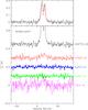 |
Fig. B.1 Spectra of the observed transitions toward 04302+2247. |
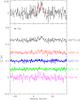 |
Fig. B.2 Spectra of the observed transitions toward AA Tau. |
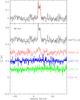 |
Fig. B.3 Spectra of the observed transitions toward AB Aur. |
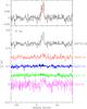 |
Fig. B.4 Spectra of the observed transitions toward CI Tau. |
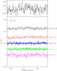 |
Fig. B.5 Spectra of the observed transitions toward CQ Tau. |
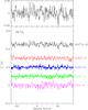 |
Fig. B.6 Spectra of the observed transitions toward CW Tau. |
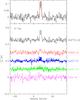 |
Fig. B.7 Spectra of the observed transitions toward CY Tau. |
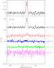 |
Fig. B.8 Spectra of the observed transitions toward DL Tau. |
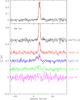 |
Fig. B.9 Spectra of the observed transitions toward DM Tau. |
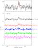 |
Fig. B.10 Spectra of the observed transitions toward DN Tau. |
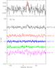 |
Fig. B.11 Spectra of the observed transitions toward DO Tau. |
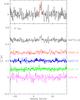 |
Fig. B.12 Spectra of the observed transitions toward FT Tau. |
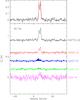 |
Fig. B.13 Spectra of the observed transitions toward GG Tau. |
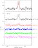 |
Fig. B.14 Spectra of the observed transitions toward GM Aur. |
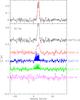 |
Fig. B.15 Spectra of the observed transitions toward GO Tau. |
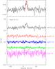 |
Fig. B.16 Spectra of the observed transitions toward Haro 6-13. |
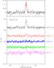 |
Fig. B.17 Spectra of the observed transitions toward Haro 6-33. |
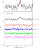 |
Fig. B.18 Spectra of the observed transitions toward Haro 6-5B. |
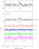 |
Fig. B.19 Spectra of the observed transitions toward HH 30. |
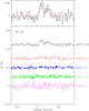 |
Fig. B.20 Spectra of the observed transitions toward HK Tau. |
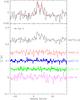 |
Fig. B.21 Spectra of the observed transitions toward HV Tau C. |
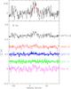 |
Fig. B.22 Spectra of the observed transitions toward IQ Tau. |
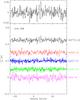 |
Fig. B.23 Spectra of the observed transitions toward LkHα 358. |
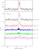 |
Fig. B.24 Spectra of the observed transitions toward LkCa 15. |
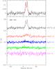 |
Fig. B.25 Spectra of the observed transitions toward MWC 480. |
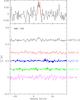 |
Fig. B.26 Spectra of the observed transitions toward MWC 758. |
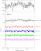 |
Fig. B.27 Spectra of the observed transitions toward RW Aur. |
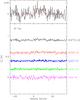 |
Fig. B.28 Spectra of the observed transitions toward RY Tau. |
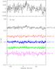 |
Fig. B.29 Spectra of the observed transitions toward SU Aur. |
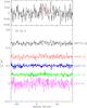 |
Fig. B.30 Spectra of the observed transitions toward UZ Tau E. |
All Tables
All Figures
|
Fig. 1 Spectra of the observed transitions toward GO Tau and DM Tau. Intensity scale is |
| In the text | |
|
Fig. 2 N = 1−0 (top) and 2−1 (bottom) C2H emission toward CI Tau, CY Tau, and GO Tau. Conversion to flux density can be obtained by scaling by 6.1 Jy/K and 7.0 Jy/K the observed spectra, respectively. The red ticks indicate the expected positions and relative intensities of the hyperfine components. |
| In the text | |
|
Fig. 3 Integrated spectra of the two groups of hyperfine components for CN N = 2−1 line, and maps of the S/N toward GM Aur (contours are in steps of 2σ). The profile of the best-fit disk model (see Sect. 4.5) is shown in red. |
| In the text | |
|
Fig. 4 Averages of the SO(65−54) and SO(67−56) spectra resampled to a common velocity scale. |
| In the text | |
|
Fig. 5 Correlation plot of the column density of molecules at 300 au with stellar luminosity, spectral type, 1.3 mm flux density and stellar age. Embedded objects appear in red, HAe stars in blue, and T Tauri stars in black. Error bars are ± 1σ with limits at 2σ indicated by arrows. |
| In the text | |
|
Fig. 6 Spectra of 12CO, 13CO, and HCO+ toward LkHα 358. Top: 12CO from the interferometric measurement of Schaefer et al. (2009). The blue curve is the fitted profile based on the disk analysis made in the uv plane. The red curve uses the same disk parameters, except for the outer radius which is 250 au instead of 170 au. Bottom: 13CO(2−1) spectrum (histogram) and HCO+(3−2) (filled histogram). The green curve is the tentative fit of a disk component from Guilloteau et al. (2013). |
| In the text | |
|
Fig. 7 Observed spectra and fitted profiles for FT Tau. The gray area is the range affected by confusion from the molecular cloud that is ignored in the CO analysis. The insert shows the integrated CO emission with contour spacings of 50 mJy km s-1 (angular offsets in arcsec). The cross indicates the position and orientation of the disk (derived from the continuum emission and kinematics pattern). |
| In the text | |
|
Fig. 8 Predicted column densities at 300 au as a function of disk midplane temperature with observed points superimposed. Color markers are DM Tau (red), GO Tau (blue), and MWC 480 (cyan). The continuous line is for “standard low metal” abundances, while the dashed line assumes an additional depletion of C and O by a factor 10. |
| In the text | |
|
Fig. 9 Predicted molecular densities at 300 au as a function of height above the disk midplane (in scale heights, defined as cs/ Ω, where cs is the sound speed, and Ω the Keplerian angular frequency). The upper panel shows the H2 density with the two horizontal and vertical lines delimiting the range where most molecules are abundant. |
| In the text | |
|
Fig. A.1 Correlation plot of the column density ratios of molecules at 300 au with stellar luminosity and spectral type, age, and 1.3 mm flux density. CN used as reference. |
| In the text | |
|
Fig. A.2 Correlation plot of the column density ratios of molecules at 300 au with stellar luminosity and spectral type, age, and 1.3 mm flux density. HCO+ used as reference. |
| In the text | |
|
Fig. B.1 Spectra of the observed transitions toward 04302+2247. |
| In the text | |
|
Fig. B.2 Spectra of the observed transitions toward AA Tau. |
| In the text | |
|
Fig. B.3 Spectra of the observed transitions toward AB Aur. |
| In the text | |
|
Fig. B.4 Spectra of the observed transitions toward CI Tau. |
| In the text | |
|
Fig. B.5 Spectra of the observed transitions toward CQ Tau. |
| In the text | |
|
Fig. B.6 Spectra of the observed transitions toward CW Tau. |
| In the text | |
|
Fig. B.7 Spectra of the observed transitions toward CY Tau. |
| In the text | |
|
Fig. B.8 Spectra of the observed transitions toward DL Tau. |
| In the text | |
|
Fig. B.9 Spectra of the observed transitions toward DM Tau. |
| In the text | |
|
Fig. B.10 Spectra of the observed transitions toward DN Tau. |
| In the text | |
|
Fig. B.11 Spectra of the observed transitions toward DO Tau. |
| In the text | |
|
Fig. B.12 Spectra of the observed transitions toward FT Tau. |
| In the text | |
|
Fig. B.13 Spectra of the observed transitions toward GG Tau. |
| In the text | |
|
Fig. B.14 Spectra of the observed transitions toward GM Aur. |
| In the text | |
|
Fig. B.15 Spectra of the observed transitions toward GO Tau. |
| In the text | |
|
Fig. B.16 Spectra of the observed transitions toward Haro 6-13. |
| In the text | |
|
Fig. B.17 Spectra of the observed transitions toward Haro 6-33. |
| In the text | |
|
Fig. B.18 Spectra of the observed transitions toward Haro 6-5B. |
| In the text | |
|
Fig. B.19 Spectra of the observed transitions toward HH 30. |
| In the text | |
|
Fig. B.20 Spectra of the observed transitions toward HK Tau. |
| In the text | |
|
Fig. B.21 Spectra of the observed transitions toward HV Tau C. |
| In the text | |
|
Fig. B.22 Spectra of the observed transitions toward IQ Tau. |
| In the text | |
|
Fig. B.23 Spectra of the observed transitions toward LkHα 358. |
| In the text | |
|
Fig. B.24 Spectra of the observed transitions toward LkCa 15. |
| In the text | |
|
Fig. B.25 Spectra of the observed transitions toward MWC 480. |
| In the text | |
|
Fig. B.26 Spectra of the observed transitions toward MWC 758. |
| In the text | |
|
Fig. B.27 Spectra of the observed transitions toward RW Aur. |
| In the text | |
|
Fig. B.28 Spectra of the observed transitions toward RY Tau. |
| In the text | |
|
Fig. B.29 Spectra of the observed transitions toward SU Aur. |
| In the text | |
|
Fig. B.30 Spectra of the observed transitions toward UZ Tau E. |
| In the text | |
Current usage metrics show cumulative count of Article Views (full-text article views including HTML views, PDF and ePub downloads, according to the available data) and Abstracts Views on Vision4Press platform.
Data correspond to usage on the plateform after 2015. The current usage metrics is available 48-96 hours after online publication and is updated daily on week days.
Initial download of the metrics may take a while.