| Issue |
A&A
Volume 592, August 2016
|
|
|---|---|---|
| Article Number | A158 | |
| Number of page(s) | 20 | |
| Section | Stellar atmospheres | |
| DOI | https://doi.org/10.1051/0004-6361/201220881 | |
| Published online | 23 August 2016 | |
Radiation-driven winds of hot luminous stars
XVIII. The unreliability of stellar and wind parameter determinations from optical vs. UV spectral analysis of selected central stars of planetary nebulae and the possibility of some CSPNs as single-star supernova Ia progenitors
Universitäts-Sternwarte München,
Scheinerstraße 1, 81679
München,
Germany
e-mail:
This email address is being protected from spambots. You need JavaScript enabled to view it.
;This email address is being protected from spambots. You need JavaScript enabled to view it.
;This email address is being protected from spambots. You need JavaScript enabled to view it.
Received:
10
December
2012
Accepted:
9
May
2015
Abstract
Context. The uncertainty in the degree to which radiation-driven winds of hot stars might be affected by small inhomogeneities in the density leads to a corresponding uncertainty in the determination of the atmospheric mass loss rates from the strength of optical recombination lines and – since the mass loss rate is not a free parameter but a function of the stellar parameters mass, radius, luminosity, and abundances – in principle also in the determination of these stellar parameters. Furthermore, the optical recombination lines also react sensitively to even small changes in the density structure resulting from the (often assumed instead of computed) velocity law of the outflow. This raises the question of how reliable the parameter determinations from such lines are.
Aims. The currently existing severe discrepancy between central stars of planetary nebulae (CSPN) stellar and wind parameters derived from model fits to the optical spectra and those derived using hydrodynamically consistent model fits to the UV spectra is to be reassessed via a simultaneous optical/UV analysis using a state-of-the-art model atmosphere code.
Methods. We have modified our hydrodynamically consistent model atmosphere code with an implementation of the usual ad hoc treatment of clumping (small inhomogeneities in the density) in the wind. This allows us to re-evaluate, with respect to their influence on the appearance of the UV spectra and their compatibility with the observations, the parameters determined in an earlier study that had employed clumping in its models to achieve a fit to the observed optical spectra.
Results. The discrepancy between the optical and the UV analyses is confirmed to be the result of a missing consistency between stellar and wind parameters in the optical analysis. While clumping in the wind does significantly increase the emission in the optical hydrogen and helium recombination lines, the influence of the density (velocity field) is of the same order as that of moderate clumping factors. Moderate clumping factors leave the UV spectra mostly unaffected, indicating that the influence on the ionization balance, and thus on the radiative acceleration, is small. Instead of the erratic behavior of the clumping factors claimed from the optical analyses, our analysis based on the velocity field computed from radiative driving yields similar clumping factors for all CSPNs, with a typical value of fcl = 4. With and without clumping, wind strengths and terminal velocities consistent with the stellar parameters from the optical analysis give spectra incompatible with both optical and UV observations, whereas a model that consistently implements the physics of radiation-driven winds achieves a good fit to both the optical and UV observations with a proper choice of stellar parameters. The shock temperatures and the ratios of X-ray to bolometric luminosity required to reproduce the highly ionized O vi line in the FUSE spectral range agree with those known from massive O stars (LX/Lbol ~ 10-7...10-6), again confirming the similarity of O-type CSPN and massive O star atmospheres and further strengthening the claim that both have identical wind driving mechanisms.
Conclusions. The similarity of the winds of O-type CSPNs and those of massive O stars justifies using the same methods based on the dynamics of radiation-driven winds in their analysis, thus supporting the earlier result that several of the CSPNs in the sample have near-Chandrasekhar-limit masses and may thus be possible single-star progenitors of type Ia supernovae.
Key words: stars: atmospheres / stars: evolution / stars: winds, outflows / stars: fundamental parameters / stars: AGB and post-AGB
© ESO, 2016
1. Introduction
The computation of a synthetic spectrum that can be compared to the observed spectrum is the primary and most important diagnostic tool for determining the fundamental parameters of a star. But while a photospheric model1 will yield information about the effective temperature Teff and the surface gravity log g, the spectroscopic determination of the radius R requires an observable quantity that can be spectroscopically traced over a depth range covering an appreciable fraction of the physical size of the star. Furthermore, a physical description is required that predicts the run of this quantity as a function of the radius.
Many stars have thin, effectively plane-parallel atmospheres, for which such a procedure is not applicable. For these stars, information in addition to the stellar spectrum, for example the measured flux and the distance to the star, is required to determine the radius. In the atmospheres of O-type stars, however, the radiative intensities are large enough for the radiation pressure to drive a stellar “wind”, propelled by the transfer of photon momentum to ions in the wind via absorption in spectral lines. The winds leave conspicuous, easily observable signatures in the stellar spectra, allowing individual spectral lines to be traced out to tens of stellar radii, thereby yielding information on the run of the velocity and density field in the wind. Strength and velocity of the outflow are not random, however. Because the acceleration of the wind is governed by the interplay of gravity and the absorption and emission of radiation in the wind, the wind parameters depend in a unique way on the stellar parameters2. Since the density and velocity in the wind can also be predicted by selfconsistent hydrodynamical modeling of the outflow on the basis of the gravitational and the radiative acceleration at each point in the wind, the comparison of observed and predicted spectra provides a link to the stellar radius and gravity, thus allowing for a purely spectroscopic determination of the stellar mass.
Central stars of planetary nebulae (CSPNs) are valuable research objects because they represent a unique phase in the evolution of intermediate-mass stars, and accurately known stellar parameters would constitute a stringent test of evolutionary models. Unfortunately, accurate distances to most CSPNs are not available, and information about their sizes (and thus, via log g, their masses) must therefore be derived either spectroscopically through hydrodynamic modeling of the expanding atmosphere or, supplemental to spectroscopy, with the aid of additional physical considerations.
Currently there exists a dispute regarding the true stellar parameters of (a selected subset of) CSPNs. This has its origins in two series of analyses of (largely congruent) samples of O-type CSPNs, using different methods. One of these (Méndez et al. 1988b,a; Kudritzki et al. 1997 (K97); Kudritzki et al. 2006 (K06)) used model fits to the optical hydrogen and helium lines to determine effective temperatures and surface gravities. Lacking hydrodynamical modeling of the wind, they had to use stellar evolutionary models to determine masses and radii, comparing effective temperatures and surface gravities to the theoretical evolutionary tracks in the Teff–log g plane. These analyses were therefore not an independent test of the evolutionary models, since their validity had been assumed all along. Nevertheless, a surprising result was that K97 found many high-mass CSPNs (with masses around 0.9 M⊙), which was unexpected, since theory predicted them to evolve too quickly to be observed in larger numbers. Still, the mass loss rates derived from their stellar parameters and from modeling of the Hα emission were well in agreement with what was expected from radiation-driven wind theory, providing strong evidence that the winds of these objects are indeed driven by radiation pressure.
The other series of analyses (Pauldrach et al. 1988, 2003; Pauldrach et al. 2004 (P04); Kaschinski et al. 2012) is based on hydrodynamic modeling of the wind, using fits to the observable UV spectra. This type of analysis had been successfully applied to massive O stars (Pauldrach 1987; Pauldrach et al. 1990a, 2001, 2012), but its application to O-type CSPNs gave even more unexpected results: P04 found a number of CSPNs with masses around 1.3 to 1.4 M⊙, near the Chandrasekhar limit for white dwarfs (Stoner 1930, Chandrasekhar 1931). These high masses, however, were not simply due to a systematic overestimate of the masses by the method. One of the stars, NGC 2392, was even found to have a surprisingly small mass of only 0.4 M⊙, compared to the 0.9 M⊙ that had been derived by K97.
Since both sets of analyses were based on different spectral regions it was not clear whether this discrepancy was due to some assumption in the modeling that was perhaps unjustified (e.g., that the winds were radiatively driven, or that the mass-luminosity relation assumed by K97 correctly described these objects), or whether there was something peculiar about either the optical or the UV spectra, despite the good fits both groups achieved for their spectral ranges. A first attempt to resolve the issue was made by Kaschinski et al. (2012) with combined optical and UV modeling from the same atmospheric models. For their analysis they chose NGC 2392, the least massive star, and NGC 6826, the most massive star in the sample of P04. These extreme cases were chosen on the premise that covering a larger spread in stellar parameters makes it more likely for the results to show real physical behavior, and not just a selection effect, in a group of stellar objects.
The results of this investigation were telling. The synthetic spectra modeled with the stellar parameters from the optical analysis could only achieve fits to the observations because the wind parameters that had been assumed in that analysis were inconsistent with the stellar parameters. Enforcing consistency between stellar and wind parameters could yield simultaneous fits to both the UV and the optical spectra, but only with stellar parameters that were in disagreement with the theoretical CSPN mass-luminosity relation. Merely the optical emission lines Hα and He iiλ 4686 could not be reproduced fully by Kaschinski et al., the emission predicted by their models being too weak.
In the present paper we will address this significant point. For the optical analyses, Hα is the primary diagnostic line for deriving mass loss rates, and reliable modeling of the Hα emission is therefore crucial to obtain accurate mass loss rates in these analyses3. In recent years4 evidence has accumulated that the winds might not be entirely smooth but clumpy (e.g., Repolust et al. 2004), and Hα, being a recombination line and thus proportional to the square of the density, would therefore show increased emission compared to that from a smooth wind. In other words, model fits assuming a smooth flow would overestimate the mass loss rates. In view of this fact, K06 reanalyzed the data of K97, adjusting clumping factors in the models to provide new fits to the optical emission lines and resulting in revised stellar parameters and significantly reduced mass loss rates. We will compare the results from our combined optical and UV analysis, now also taking clumping into account, to these revised parameters.
Further information about the nature of O-type CSPN winds is provided by X-ray observations (Guerrero et al. 2000; Kastner et al. 2012) that show CSPNs as X-ray emitters. This radiation is thought to originate, as in massive O star winds, from small packets of the gas that are accelerated5 relative to the mean flow and collide with other gas fragments further out, resulting in small shocked regions (with a volume filling factor of around f ≃ 10-2) of hot gas (T ≃ 106 K) that cools radiatively, emitting radiation in the X-ray regime (Lucy & White 1980; Lucy 1982). Apart from direct observation these X-rays can also be inferred from lines of highly ionized species (N v, O vi, and S vi) in the observable UV region. The presence of such highly ionized species (so-called superionization; Snow & Morton 1976) could be readily explained by shocks being the source of the high-energy radiation required to generate these ions. Some of their lines lie in the FUSE spectral range, and corresponding observations exist for several of the CSPNs in our sample. We use these observations to ascertain whether CSPN winds differ from massive O star winds with regard to shock radiation.
In this paper we reanalyze the sample investigated by K97. In the following we will briefly review the pros and cons of the two spectral analysis techniques (UV and optical) (Sect. 2) and discuss our modeling of the shocks to provide constraints on the radiation leading to the production of O vi (Sect. 3). Then we will describe our implementation of clumping, providing reference comparisons to the modeling code that had been used by K06, and we show comparisons to the observations of the synthetic spectra from our model runs, using the parameters of both K06 and P04, including and excluding clumping (Sect. 4). Finally, we discuss the implications of our findings in Sect. 5.
2. Methods for the investigation of CSPN winds and the determination of stellar parameters
At present there exist two major approaches to the spectral analysis of hot stars with expanding atmospheres, and which correspond to the two series of analyses referred to above. The first treats the determination of the atmospheric structure as an optimization problem by parametrizing the velocity law and attempting to find the best solution by varying the parameters and choosing the set that results in the best fit to the observed spectral line profiles. The second treats the determination of the structure of the atmosphere as a problem in hydrodynamics, which can be solved using basic physics once the state of the gas and the radiation field is modeled in sufficient detail to enable the computation of the forces acting on each volume element of the atmosphere.
2.1. Details of the methods
Parametrized method to fit the spectra of CSPNs.
This method has traditionally been the domain of optical spectral analysis, but it can be extended to include the UV as well (e.g., Herald & Bianchi 2011). In the analysis of the optical spectrum, the effective temperature Teff is obtained from NLTE model fits to the optical He i and He ii stellar absorption lines and the surface gravity log g is derived from fits to the Balmer lines (mainly Hγ, but also Hβ; see Méndez et al. 1988b, K97). The velocity of the outflow in the wind region is parametrized with a “beta velocity law”, v(r) = v∞(1 − bR/r)β, where the best-fit value of β is to be found as part of the analysis, and the parameter b fixes the velocity at the inner boundary of the wind, usually taken to be of the order of the sound speed. The terminal wind velocity v∞ can normally be measured directly from the observed blue edge of the saturated P-Cygni profiles in the UV spectrum6. This velocity law is then connected in a smooth transition to the hydrostatic density structure in the deeper atmospheric layers. The mass loss rate Ṁ that determines the wind density via the equation of continuity, ρ(r) = Ṁ/ (4πr2v(r)), is determined via a model fit to the Hα emission profile (see, e.g., K06)7.
The realization that the winds may not be entirely smooth has given a provisional explanation to the fact that with a model assuming an unclumped flow it was not always possible to simultaneously fit all emission lines in the optical, and thus some form of ad hoc treatment of clumping (such as the one described in Sect. 4) is nowadays often used with this method to improve the fit to the spectrum.
Consistent hydrodynamic method for determining complete sets of stellar parameters for CSPNs.
Taking into account the relevant forces and actually solving the equation of motion eliminates the need to assume a velocity law. The solution provides not only the structure of the velocity field and the terminal velocity, but also the density (and thus, the mass loss rate) in a unified way throughout the entire atmosphere, from the hydrostatic layers deep in the photosphere to the outer regions of the wind where the forces become negligible and the terminal velocity is reached.
A distinctive characteristic of the method is that the mass loss rate and the terminal velocity that satisfy the constraint of self-consistency are determined in dependence of the stellar parameters. Since the UV spectrum varies characteristically as a function of these wind parameters (see, e.g., Fig. 5 of Pauldrach et al. 2012), this dependence can be used diagnostically to determine the stellar parameters from the appearance of the UV spectrum8. For a more detailed discussion of the numerical procedures used to implement this method we refer the reader to Pauldrach et al. (2012) and Pauldrach et al. (2001)9.
A complete hydrodynamically self-consistent model usually requires some iteration scheme, beginning with a plausible guess of the line force for a given set of stellar parameters. Using this initial guess, the hydrodynamical structure is computed and the NLTE problem (i.e., radiative transfer with consistently derived rate equations and occupation numbers, and corresponding opacities and emissivities) is solved. From this solution, new values for the radiative forces are calculated, and the procedure is iterated until convergence is achieved. The radiative force is computed analogously to the synthetic spectrum using the same occupation numbers and radiation field, and the quality of the fit of the spectrum is thus also a measure of the accuracy of the computed line force. If the spectral fit of the converged model is not satisfactory, new stellar parameters are chosen and the process is repeated.
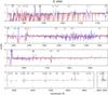 |
Fig. 1 Observed UV and optical spectrum of IC 4593 (gray) compared to synthetic spectra computed from atmospheric models with consistently calculated winds, based on the stellar parameter sets of Kudritzki et al. 2006 (K06c; blue) and Pauldrach et al. 2004 (P04; red). The K06c spectrum shows large differences to the observed spectrum, thus arguing against this parameter set, whereas the P04 spectrum is in generally much better agreement with the observed spectrum. (For cosmetic reasons, and to identify and distinguish the interstellar lines from the stellar features, the most important interstellar lines (primarily absorption by molecular and atomic hydrogen) have also been included in the latter model12.) The plot also illustrates the well-known fact that the UV spectrum of O stars contains much more, and stronger, spectral lines than the optical. Given the furthermore known sensitivity of the optical emission lines to physical and modeling uncertainties such as clumping (to which the UV spectrum is much more robust), this emphasizes that the UV carries much more diagnostic weight than the optical. |
For example, if the calculated terminal wind velocity v∞ of a model differs from the observed one, M has to be modified until agreement is reached (since v∞ scales with (M/R)1/2 according to the theory of radiation-driven winds); if the predicted spectrum then differs from the observed one, Ṁ needs to be modified via a change of R (since log Ṁ ~ log L, according to radiation-driven wind theory). But the change in R also forces one to change the mass M again, in order to keep v∞ consistent with the observed value. Using a sequence of new models10 computed this way the process is repeated until a good fit to the observed spectrum is obtained. (Teff might also be corrected slightly during this iteration, by computing models for a series of temperatures and choosing the one that fits the Fe iv/Fe v ionization balance best. This procedure usually allows the effective temperature to be constrained to within ± 1000 K11, cf. Pauldrach et al. 2004, 2001.)
2.2. Discussion
Given that both methods can be used as a basis for computing synthetic spectra, it may be tempting to assume that both methods are therefore also of similar utility for determining stellar parameters from the analysis of observed spectra. This is not the case, however.
The parameter-fitting approach cannot be used for a purely spectroscopic determination of the radii and masses (which is necessary for the objects considered here, on account of their uncertain distances) because it does not consider the physical constraints imposed by the processes responsible for driving the expansion of the atmosphere. For any set of stellar parameters it allows the user to arbitrarily select a mass loss rate and terminal velocity, without regard for whether a star with the given stellar parameters could actually drive such a wind. The fact that a fit to the observed optical emission lines (whose profiles are determined to a large extent by the mass loss rate) may be obtained with suitably selected wind parameters cannot be regarded as confirming a chosen radius: because all parameter combinations leading to the same value of Q = Ṁ/ (Rv∞)3/2 result in similar recombination line profiles (e.g., Puls et al. 2005), for any other given radius a different mass loss rate can be found that also reproduces the same lines.
In contrast, determining which wind strength and velocity will physically result from a given set of stellar parameters is the key principle of the hydrodynamic method. Together with the realization that both mass loss rate and terminal velocity have a characteristic influence on the appearance of the UV spectrum, this dependence may be used “in reverse” to find, using a suitable grid of models of different masses and radii, that set of stellar parameters whose computed wind properties and resulting UV spectrum offers the best fit to the observed spectrum.
This does not necessarily mean that the agreement between the predicted spectrum and the observed one will be perfect in all details – nor would we expect it to, given that it is very unlikely that all CSPNs would exhibit exactly the same identical surface abundance pattern that is our current best interpretation of our sun’s composition, and which is used by default in the models13. But even without elemental abundance fine-tuning a grid of models will show, as a function of the stellar parameters, a well-defined optimum14 in the fit of predicted and observed spectrum, due to the unique way that both the terminal velocity and the mass loss rate – and thus the appearance of the UV spectrum – depend on mass and radius of the star; and since the dependences are monotonic, no further optimum exists.
As illustrated by Fig. 5 of Pauldrach et al. (2012) – which shows the appearance of the visible UV spectrum as a function of radius and surface gravity (or, equivalently, radius and mass) for a set of dynamically consistent models – the velocity field, the mass loss rate Ṁ, and the synthetic spectrum depend in a sensitive way on the values chosen for the parameters Teff, M, and R of a model atmosphere.
In this context it is not crucial that the mass and radius range of this “normal” O star sample differs from that of our CSPN sample because the UV-spectra of our CSPNs are very similar to those of massive O stars. The reason for this behavior is given by the theory of radiation-driven winds, according to which similar solutions for the velocity field (v∞ ∝ (M/R)1/2) and the characteristic wind density (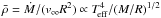 , cf. Pauldrach et al. 1990a) are obtained for the CSPNs as for the massive O stars. This is the decisive point because the formation of the UV-spectra is primarily ruled by these values (cf. Puls & Pauldrach 1991; and Kaschinski et al. 2012). The winds of our CSPNs are therefore of comparable strength to those of massive O stars15.
In view of this consideration we can thus exemplify the sensitivity of the procedure using the computed UV-spectra shown in Fig. 5 of Pauldrach et al. (2012). The models shown in the first row have masses only 20% smaller than the corresponding models of the second row, while the radii and effective temperatures are the same (see also Fig. 2). Because the spectra change significantly even for these small changes in the stellar mass, our assessment that the stellar mass can be determined in this way to within about 10% is readily understood. (Disregarding, of course, possible but yet unknown systematic peculiarities of individual stars.)
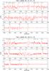 |
Fig. 2 Excerpt of Fig. 5 of Pauldrach et al. (2012) showing the appearance of the visible UV spectrum of massive O stars as a function of mass M for a constant effective temperature Teff and radius R, resulting from dynamically consistent wind models. (Teff = 40 000 K, R = 15 R⊙, and solar abundances have been assumed for the models.) Although the mass of the first model is only 20% smaller than that of the second one, the resulting UV spectra appear markedly different. Because of this strong response, the UV spectrum can be used diagnostically for a determination of the stellar mass. A corresponding dependence of the appearance of the UV spectrum on the stellar parameters as shown here for massive O stars also holds for O-type CSPNs, which have comparable wind densities and velocities (see text), and thus similar UV spectra. |
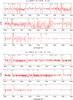 |
Fig. 3 Appearance of the UV spectrum for two dynamically consistent CSPN models with different stellar parameters (as labeled), illustrating the strong reaction of the UV spectrum to changes in the stellar parameters. Because of this sensitive dependence, the UV spectrum can be used diagnostically for a fine-grained determination of the stellar parameters, in particular the masses. |
In summary, a good fit to the observable UV spectrum can be achieved only with a unique stellar parameter set, and due to the strong response – as also illustrated in Fig. 3 for two CSPN models representative of a condensed form of Fig. 5 of Pauldrach et al. (2012) – of the UV spectrum to even small changes in the stellar parameters used, these can be determined quite precisely. In particular, the spectrum changes for models in the CSPN mass range visibly even for small absolute changes in the stellar mass of about 0.1 M⊙, so that the uncertainty in the derived stellar masses is, as already noted by Pauldrach et al. (2004), usually very small (~0.1 M⊙; cf. Fig. 3). (Again, of course, disregarding potential systematic differences.)
This sensitivity of the method, based on the response of the observable UV spectrum on not only the velocity field but via the characteristic wind density also on the optical depths in the wind, thereby represents an improvement over that achievable solely from the predicted mass-loss rate and the dependence of the predicted v∞ on the mass16, combined with the good accuracy with which v∞ can be measured from the observed spectrum (~10%), which together would allow the masses to be determined to within about 20%, as estimated from Figs. 5 and 6 of Pauldrach et al. (1988).
Because the aim of the current paper is the assessment of the compatibility of stellar parameter sets with the observed spectra rather than abundance fine-tuning17, for the purposes of the present analysis it is therefore sufficient to present the predicted spectra on a scale where the response of the spectrum as a result of varying the stellar parameters becomes visible. Depending on the differences in masses and radii, the differences in the resulting spectra can become quite pronounced. Comparing, for example, the spectra shown in red and blue in Fig. 1, it is evident that one of them clearly represents a much better fit to the observed spectrum than the other. Also noticeable is that there are no particular selected features that react to the changing mass loss rate; rather, all lines in the UV respond in varying degrees to the changes.
Ultimately, of course, the question of the true parameters of the selected CSPNs will likely only be resolved with the availability of an entirely independent determination of the radii, such as will hopefully become possible with the distance determinations through Gaia (and by which the models may be calibrated to then allow purely spectroscopic parameter determinations for even more distant stars). If, given these independent stellar parameter determinations, our predictions were to turn out wrong this would certainly be disconcerting, but it will then have indicated a critical flaw or incompleteness in a theory which we believe to have understood in its fundamental aspects, and thereby the discrepancies may teach us more about the physics of radiation-driven winds than what we can learn by applying methods based on parametrizations without causal relationships.
The point we wish to make in this paper, however, is that we can see no urgent reason to distrust the current state of radiation-driven wind theory, and that in fact all aspects of the observations may be understood in the context of this theory if one accepts that some of the stars in our selected sample of CSPNs have perhaps not followed the canonical theoretical evolutionary path.
2.3. Models presented in this paper
In this paper we present synthetic CSPN spectra and line profiles computed on the basis of the stellar parameters from the aforementioned published analyses: (a) using the stellar parameters and the corresponding consistently computed wind parameters from P04 (models “P04”); (b) using the stellar parameters from K06 with consistently computed wind parameters (models “K06c”); and (c) using the stellar parameters from K06, but with line force parameters artificially fitted so as to reproduce the mass loss rates and terminal velocities published by K06 (models “K06f”) – these latter models are in general not hydrodynamically consistent except by happenstance; we use them only to compare with line profiles published elsewhere, but we do not consider them to represent possibly existing objects.
We note that although our K06f models have the same mass loss rates and terminal velocities as the models presented by K06, they are not identical, because the velocity field in the wind – and therefore also the density as a function of radius – differs (the former use a hydrodynamically computed velocity field with the line force adjusted to yield the desired Ṁ and v∞, while the latter assume a beta velocity law). As we find below, however, these small differences are sufficient to introduce differences in the synthetic optical emission line profiles of a similar magnitude as the proposed wind clumping would. For this reason we must currently consider the numerical values of clumping factors derived using fits to the observed optical emission lines on the basis of an assumed beta velocity law (apart from the generally unverified hydrodynamical consistency of the wind parameters) to be arguable.
2.4. Further constraints
Further constraints on the nature of the driving mechanism of CSPN winds are offered by two other avenues of investigation. First, via a study of the behavior of the wind dynamics independent of the appearance of the spectra; and second, via modeling of the X-ray emission in the winds.
Regarding the first point it is important to keep in mind that the wind parameters are functions of the stellar parameters. Thus, if the wind parameters predicted for a set of stellar parameters contradict the observations, these stellar parameters are likely to be wrong. Such an inconsistent behavior can, for example, be evident in the ratio v∞/vesc of the terminal wind velocity and the escape velocity of individual stars. In a previous paper (Kaschinski et al. 2012) we had examined the v∞/vesc ratios for both the consistent, UV-derived stellar parameter set of our CSPN sample as well as one based on optical emission lines and the theoretical post-AGB mass-luminosity relation. The results showed that the spread in the v∞/vesc ratios of the former set turned out to be comparable to that obtained from both massive O star observations and massive O star models, whereas the v∞/vesc ratios of the latter set yielded values that were much too high and incompatible with all other results. As this anomaly is coupled to the fact that the escape velocity vesc is not a directly observable quantity18, we concluded that there is a problem with the mass-luminosity relation at the CSPN high-mass end.
Although this is a remarkable result, it might possibly be construed as an intrinsic peculiarity of CSPN winds not exhibited by massive O star winds. It is therefore significant that the treatment of the expanding atmospheres of O-type stars offers another, independent, path of inquiry into the driving mechanism of CSPN winds, via the modeling of the wind-produced X-rays. This is based on the hydrodynamical behavior of radiation-driven winds and can thus be used as a further test of the reliability of the calculated wind dynamics.
As the X-rays are produced as a second-order effect by the cooling zones of shocked material within the winds, arising from the unstable, non-stationary behavior of the radiative wind driving mechanism (Lucy & Solomon 1970; Owocki & Rybicki 1984), besides being observable directly, this radiation can also be observed indirectly via its influence on the ionization balance. In particular, it leads to the production of higher ionization stages such as O vi (e.g., Pauldrach 1987; Pauldrach et al. 1994b), which can be observed by means of the well-known O vi resonance doublet λλ 1031, 1037. To strengthen or weaken the general finding that CSPN winds are radiatively driven it is thus expedient to model the O vi line in the CSPN spectra and thereby to quantify the X-ray production rate and the radial distribution of the X-ray emitting gas, as has already been done for massive O star atmospheres (Pauldrach et al. 1994a,b, 2001, 2012).
3. Extended UV analysis of a selected CSPN subset
To investigate the influence of X-rays on the synthetic UV spectra of CSPNs and to analyze their characteristics we present in the following an extended UV analysis of a selected sample of CSPNs, based on a comparison of our synthetic UV spectra with HST and IUE observations, and also with corresponding FUSE observations which include the wavelength range of the O vi resonance line. This spectral line is primarily produced by Auger ionization driven by X-rays emitted by the shock cooling zones resulting from the unstable, non-stationary behavior of the winds, and thus represents a special diagnostic tool for these shocks by allowing their consequences to be analyzed from observations in the UV spectral range, in particular regarding the quantity and the structure of the X-rays (Pauldrach et al. 1994b, 2001, 2012). With the FUSE data available this diagnostic potential of the O vi line can be utilized for six CSPNs of our sample: NGC 2392, IC 4593, IC 418, Tc 1, NGC 6826, and He 2-131.
For these six CSPNs we list in Table 1 the masses and wind parameters (all other stellar parameters of these objects are given in Table 2) for the P04 and the K06c model series. Examples of comparisons of the UV spectra from WM-basic model runs to the observations are shown in Figs. A.1 through A.4 for the four CSPNs NGC 2392, IC 4593, IC 418, and NGC 6826. The O vi line in the spectra of Tc 1 and He 2-131 is very similar to that of IC 418 (Fig. A.5) in spite of differences in the terminal velocity, which is thus seen not to play a crucial role in the formation of this line. We thus expect (without having verified this with detailed model runs) similar values of the X-ray parameters for these two stars as for the other ones.
Stellar masses and wind parameters for the six selected stars of our sample of CSPNs for which FUSE observations are available.
NGC 2392.
The middle panel of Fig. A.1 shows the synthetic UV spectrum of our standard P04 model of NGC 2392. The predicted spectrum is generally in good agreement with the observed IUE spectrum, and also with the FUSE observations. (We expect the minor deviations seen in some spectral lines to be correctable by adjusting the corresponding abundances slightly. However, such fine-tuning is beyond the scope of our present investigation19.) The observed O vi line, however, is clearly not reproduced by the synthetic spectrum, and this indicates that – as in massive O stars – X-rays are also an important ingredient in CSPN winds. As X-rays are produced by shock cooling zones embedded in the wind, the physics that describe this phenomenon must thus be applied to CSPN models in the same manner as it has been applied to the models of massive O stars20.
Overview of models for the nine CSPNs of the investigated sample.
In the lower panel of Fig. A.1 we show the synthetic spectrum from our model of NGC 2392 in which we have included shocks in this manner. The spectrum now reproduces the profile of the O vi P-Cygni line quite well, and as an integral part of the modeling procedure we obtain the emitted frequency-integrated relative X-ray luminosities21LX/Lbol as well as the radial distribution of the maximum local shock temperatures22Ts(r) in the cooling zones of the shock-heated matter component (Table A.1).
While the synthetic spectrum of our current best model (P04 plus shocks) is now quite well in agreement with the complete observed UV spectrum – the IUE and HST observations along with the FUSE data –, the same cannot be said of the K06c model shown in the upper panel, which does not at all reproduce the observations. This is mainly due to the much too high mass loss rate resulting from the stellar parameters of that model (although the resulting terminal velocity is close to the observed value). Because spectra computed from models using consistent wind dynamics but based on stellar parameter sets obtained from optical analyses had shown large discrepancies to observed spectra (in the optical as well as in the UV) in the past, Kaschinski et al. (2012) had already concluded that the published optical analyses give good fits to the observed spectrum only because the wind parameters assumed in these analyses are inconsistent with their stellar parameters. With regard to the comparison shown in the upper panel of Fig. A.1 we reach the same conclusion here (see also the upper panels of Figs. A.2 through A.4).
IC 4593, IC 418, and NGC 6826.
Our findings and conclusions for NGC 2392 apply similarly to the central stars of IC 4593, IC 418, and NGC 6826. As is shown in the lower panels of Figs. A.2 through A.4 the O vi lines of these stars are, along with the rest of the spectra, quite well reproduced by our method and especially by our treatment of the shock physics (see also Fig. 1). (The parameters that describe the behavior of the shocks, deduced from the analysis of the O vi line, are shown in Table A.1.) In contrast to this, the upper panels of Figs. A.2 through A.4 show the synthetic UV spectra of the K06c models, which exhibit a much poorer agreement with the observed spectra. (Considering the bad matches to the observed spectra we did not think it meaningful to also apply the treatment of shocks to these models.) As in the case of NGC 2392 the primary reason for the mismatch is that these stellar parameters result in mass loss rates that are too high to describe these objects accurately. But in contrast to the model of NGC 2392 the obtained terminal velocities are also too small for these three CSPNs. This is an additional strong hint that something is wrong with the stellar parameters of these models (parameter sets K06c in Table 1) – and this certainly applies to the stellar masses, which for these sets have not been determined spectroscopically but assumed.
Discussion of the characteristic values of the X-ray emission.
The model used to simulate the behavior of shocks constrained by the appearance of the O vi line also yields the radial distribution of the maximum local shock temperatures and particularly the integrated X-ray luminosities, which can be compared to the observationally deduced values. Kastner et al. (2012) have presented results obtained from the first systematic Chandra X-ray Observatory survey of planetary nebulae (PNe) in the solar neighborhood (within ~1.5 kpc). The highlights of these results include the finding that roughly 50% of the PNe observed by Chandra harbor X-ray-luminous CSPNs, and that this fraction involves detections of diffuse X-ray emission and detections of X-ray point sources. (The diffuse X-ray emission is thought to arise from shells where the CSPN wind rams into the previously expelled asymptotic giant branch (AGB) envelope, producing hot shocked gas; the point-like sources are associated with the central stars themselves.) Most noticeable is that five objects, including NGC 2392, display both diffuse and point-like emission components in the Chandra imaging. From an observational point of view it would therefore be worthwhile to disentangle the contributions of the two sources.
In this regard it is quite interesting that Guerrero et al. (2005) derived for the central star of NGC 2392 and its surrounding Eskimo Nebula at our distance of 1670 pc an X-ray luminosity of LX = (2.6 ± 1.0) × 1031·(1670/1150)2 erg s-1 = 5.4 × 1031 erg s-1 which is almost exactly a factor of two larger than the value LX = 2.3 × 1031 erg s-1 we have deduced from our best-fit model for this CSPN (see Tables 1 and A.1). This agrees with the observational results of Kastner et al. (2012 see their Fig. 3), and also with the interpretation of Guerrero et al. (2005) of their result: They noted that the X-ray emission of NGC 2392 has to be partially attributed to the central star and partially to the diffuse X-ray emission produced by the dynamical interaction of the fast outflow with the inner shell of the PN. As Chandra has detected a relatively hard point source emission in NGC 2392 (Kastner et al. 2012), which likely explains the energy dependence of the X-ray morphology apparent in the earlier XMM data (Guerrero et al. 2005), the significance of this encouraging result can certainly be underscored by a comparison of the maximum shock temperatures. The best-fit model of Kastner et al. (2012), overplotted on the EPIC/pn spectrum in their Fig. 2, has a plasma temperature of around 2.0 × 10⁶ K, which is somewhat larger than our value of 1.4 × 10⁶ K (see Table 1). But given that the highest values of the temperature of the shocked gas are likely to be associated with the highest arising Mach-numbers, which are expected to be found in the diffuse component and not the point source, we therefore regard our maximum shock temperature to be also in accord with the current observations.
Our general finding that the X-ray to bolometric luminosity ratio for CSPNs is in the range LX/Lbol ~ 10-7...10-6 (see Table 1) is further confirmed by Guerrero (2006), who deduced for the central star of NGC 6543 a value of LX/Lbol ~ 10-7 from observations. As such values of LX/Lbol are typical for radiation-driven winds – they are of the same order as observed for massive O stars (Sana et al. 2005, 2006) −, this is again a strong indication that radiation pressure determines the atmospheric structure not just of massive O stars but also of O-type CSPNs; and besides the primary behavior that rules the values of the mass loss rate Ṁ and the terminal velocity v∞, this also regards weak and secondary effects that rule the details of the shock physics.
Our consistent procedure and the corresponding analysis is thus not only based on the high radiation flux density of CSPNs (that necessarily leads to expanding atmospheres), the empirically backed wind-momentum–luminosity relation (WMLR), and the behavior of v∞/vesc, which can be compared to observations (see P04 and Kaschinski et al. 2012), but also on secondary effects such as the maximum shock temperatures and the integrated X-ray luminosities which are also accessible to observations. All these findings support the hypothesis that the atmospheres of CSPNs are governed by exactly the same radiative line-driving mechanism as those of massive O stars.
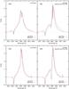 |
Fig. 4 Comparison of Hα line profiles predicted by fastwind (red) and WM-basic (black). To focus the comparison on the NLTE modeling and the treatment of radiative transfer, these WM-basic calculations use the density structures from the fastwind models. Top row: Teff = 50 000 K test model (S50), bottom row: Teff = 35 000 K test model (S35). Left panels: profiles from a smooth, unclumped flow (fcl = 1), right panels: profiles from a clumped flow (fcl = 81) with a correspondingly reduced mass loss rate (by a factor of |
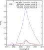 |
Fig. 5 Hα line profile of the S35 test model as in Fig. 4, but this time also showing the case of a clumped wind (fcl = 81, as in Fig. 4) with the “normal” mass loss rate (blue). Compared to this strong response, the small differences between two corresponding fastwind (red) and WM-basic (black solid line) predictions are insignificant. |
4. Accounting for clumping
Although the spectrum in the optical wavelength range is also computed by our code, it is not our means of spectral diagnostics because compared to the UV spectral range it contains only a few and only rather weak subordinate lines (see Fig. 1) which due to their weakness are not only much more susceptible to uncertainties in the modeling than the lines in the UV, but moreover may be influenced (in particular Hα and He iiλ 4686) by second-order effects possibly connected to small inhomogeneities in the density. Such inhomogeneities, leading to stronger emission from H and He recombination lines due to the higher densities in the “clumps” compared to a smooth outflow, may be the reason that Kaschinski et al. (2012) could not fit the Hα and the He iiλ4686 emission lines as well as the rest of the spectrum.
Inhomogeneities, in fact, are the currently favored explanation for such discrepancies. They are often described using ad hoc “clumping factors” employed in the models to bring the predicted Hα and He iiλ4686 lines into agreement with the observed profiles. But there is a certain caveat attached to this treatment. Supposing that clumping (or some other effect with similar influence on these two lines) does play a role, then – as long as we have no consistent physical description for this effect – this treatment allows us to obtain good fits to individual emission line profiles while providing no further insight into the stellar parameters23. A line whose model profile is determined primarily by fitting factors and not the underlying physics of the model, however, loses its diagnostic value, and the quality of the fit of this line says nothing about the reliability of the fundamental model parameters. The procedure furthermore involves the risk of covering up weaknesses in other parts of the model description (such as simplifying assumptions made for the velocity field, for example).
We therefore caution against reading too much into the deviations of these few lines, and at the present stage we consider it debatable whether the affected hydrogen and helium lines should be regarded as meaningful observables from which reliable information about the stellar and wind parameters can be deduced. On the other hand, a consistent theory of clumping is only required if the affected spectral lines are actually used diagnostically to constrain the basic model parameters. For our present purposes this is not the case: the models are constrained by the physics of radiative driving and the appearance of the UV spectra. Thus, on the basis of the primary influence of the (independently predicted) velocity field, these lines may possibly still be used to quantify the influence of small inhomogeneities on the shapes of the affected lines.
We investigate in the following whether wind clumping may constitute a plausible explanation for the fact that the models of Kaschinski et al. (2012) based on a hydrodynamically consistent smooth outflow could not reproduce the strength of the optical emission lines Hα and He iiλ 4686. We investigate further to which degree this would influence the UV spectra on which the parameter determinations had been based. For our investigation we consider a simple ad hoc description of clumping similar to that employed by others, which is in particular also implemented in fastwind (Puls et al. 2006), the model atmosphere code that had been used by K06 in their analysis.
In this “microclumping” description the gas is considered to be swept up into small, optically thin clumps with a volume filling factor of 1 /fcl(r) and void interclump regions. The density in the clumps, 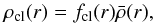 (1)is then the local clumping factor fcl(r) times the density
  of the smooth, unclumped flow given by the equation of continuity,
 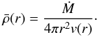 (2)The void interclump regions do not influence the radiative intensity, and only the fraction 1 /fcl of volume that actually contains matter contributes to the opacity and emissivity along a macroscopic path element. Thus, if κ = χ/ρ denotes the opacity per unit mass, the optical depths
 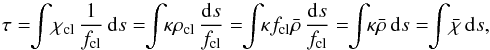 (3)and indeed all quantities that are linear in the density, remain unaffected by this clumping except that clumping may lead to a shift in the ionization stages, and thus a change in κ, through increased recombination in the higher-density clumps. On the other hand, quantities that are proportional to the square of the density, such as the emissivities of recombination lines, are enhanced by a factor of fcl compared to an unclumped flow with the same mean density.
To demonstrate that our clumping treatment in WM-basic produces results comparable to fastwind, we show in Fig. 4 the predicted Hα line profiles24 for two stellar models with strong winds (in which Hα is most likely to be affected by clumping). We use, here as well as in the CSPN model calculations of Sect. 4.1, the same radial run of the clumping factors as used by K06 in their analysis (J. Puls, priv. comm.): no clumping (i.e., fcl(r) = 1) in the photosphere and up to v = 0.05v∞; a steep rise to the specified clumping factor from v = 0.05v∞ to v = 0.1v∞; and then keeping this value fcl(r) = const for v> 0.1v∞. To focus the comparison on the clumping and the radiative transfer we have set up the comparison runs as closely as possible, in particular we have used the density structures of the fastwind models in the WM-basic test calculations. The remaining small differences in the predicted line profiles are due to actual differences in the modeling, such as the use of different model atoms, or the different interpolation of the opacities and emissivities between the grid points in the radiative transfer.
These small differences in the predicted line profiles are not relevant, however, for the purposes of diagnosing clumping factors from given observed profiles. This is shown in Fig. 5 where we compare the predicted Hα line profiles from an unclumped wind and from a clumped wind (fcl = 81) with the same mass loss rate. (The latter is equivalent to an unclumped wind with a mass loss rate increased by a factor of  .) Compared to the strong response of the profile to a change in the mass loss rate or clumping factor, the differences in the predictions of WM-basic and fastwind are small. In other words, for a given clumping factor one would deduce exactly the same mass loss rate from an observed Hα profile when using the WM-basic model as when using the fastwind model.
In these tests (and these tests only) we have used the density structures from the fastwind models in our WM-basic calculations. We specifically emphasize this point, since we have demonstrated here that both codes produce equivalent line profiles if given the same input. This is important to keep in mind in assessing the model calculations for individual CSPNs below: when using the stellar parameters of K06 (models K06f), if we do not achieve as good a fit to the observed profiles as they did, even when enforcing their mass loss rates and terminal velocities in our models, then this is not because the codes a priori produce different results, but because a different density structure was used. But that is the entire point of using our modeling code in these analyses: to base the model predictions on a density structure that follows from a solution to the equation of motion of the wind, instead of simply assuming a certain parametrization25 as K06 did. For the Hα line profile formation the differences between the assumed and the computed wind density structures play at least as important a role as the proposed clumping.
4.1. Model calculations for individual CSPNs
Here we present a comparison of observed and computed optical line profiles for our sample of nine CSPNs. For each CSPN we show the results from three different model runs (the parameters of all models are listed in Table 2): P04: stellar and (consistent) wind parameters from P04; K06c: stellar parameters from K06 and wind parameters consistent with those stellar parameters, as determined by our hydrodynamic calculations of the radiative driving force; and K06f: stellar parameters from K06, artificially enforcing their wind parameters in our model runs. For those objects where K06 have given a non-unity clumping factor we show all line profiles both including and excluding clumping. Additionally we present redetermined clumping factors derived from a comparison of the observed optical lines to our predicted optical lines obtained from the P04 models.
NGC 2392.
The central star of NGC 2392 is of particular interest as it has a mass of only 0.41 M⊙, making it the least massive CSPN of our sample. A clumping factor of 1 was derived by K06, corresponding to an unclumped wind. Unfortunately we lack observations for many of the optical lines for which we show synthetic line profiles in Fig. A.6. The computed line profiles, both in absorption and emission, for the consistent P04 and the fitted K06f models are almost identical. Both models fail to reproduce the strong Hα and He iiλ 4686 emission lines but match the absorption lines equally well. The consistent K06c model has a mass loss rate that is much too high, reflected in a too strong emission of all emission lines, and even showing Hγ in emission. Table 2 shows this huge discrepancy in the mass loss rate which is higher by a factor of 10 in the K06c model compared to the K06f model.
As the consistent P04 and the fitted K06f model both fail to reproduce the strong Hα and He iiλ 4686 emission lines, we have redetermined the clumping factor for the P04 model from a comparison of the observed optical lines to our predictions. We obtain a clumping factor of 8, a strong deviation to the result of K06 (see Table 2). The derived clumping factor represents a compromise between the predictions for the He iiλ 4686 line and the Hα line: a higher clumping factor could have reproduced the observed height of the He iiλ 4686 line better, but then the width of the predicted Hα line would have exceeded that of the observed profile (dash-dotted red line in Fig. A.6). This is a clear indication that the physical effect that enhances the emission in these two lines and which we model with the clumping approach does not quite behave, in particular with regard to its radial run, as the simplistic description applied at the present stage.
IC 4637.
For IC 4637 a clumping factor of 4 was derived by K06. The resulting synthetic optical line profiles from the P04 and the (inconsistent) K06f models match the observations for IC 4637 (Fig. A.7), and both clumped and unclumped wind result in nearly the same profiles (for Hα, the unclumped P04 model even shows a better fit than the clumped one). The consistent K06c model shows a mostly equally good fit to the absorption lines, but its high emission in Hα and He iiλ 4686 makes the K06 stellar parameters incompatible with the observations.
NGC 3242.
NGC 3242 is the only CSPN of the sample for which the UV analysis of P04 and the optical analysis of K06 yield almost the same mass, and the K06f parameter set is consistent (and thus identical to the K06c model). Both the P04 and the K06f/K06c models give nearly identical fits to all observed optical line profiles (Fig. A.8). The effects of clumping are marginal, as neither Hα nor He iiλ 4686 are in emission.
IC 4593.
For IC 4593 the situation is somewhat similar to that of IC 4637: the observed optical absorption lines are matched equally well by the P04 and the (inconsistent) K06f models (Fig. A.9). The predicted emission in Hα and He iiλ 4686 is a bit too low for both models, but with some cosmetics, i.e., a slightly larger clumping factor, the P04 model would show a perfect fit to both lines. The consistent K06c model again produces too strong emission, even without clumping, and thus rules out the K06 stellar parameters.
IC 418.
IC 418 is of special interest because K06 have found a clumping factor of 50 (!) for this star, which is by far the highest value, but even with this large clumping factor the K06f model fails to reproduce the observed Hα profile (Fig. A.10). The consistent model K06c produces much too strong emission and thus gives incompatible line profiles for all observed lines, with and without clumping. (Additionally, it results in a terminal velocity of only 200 km s-1, which is much too small compared to the observed terminal velocity of 700 km s-1.) For the P04 model, this clumping factor is also much too large, but a moderate clumping factor of 4 yields with respect to a compromise of the strength and width of the emission lines of Hα and He iiλ 4686 the best fit to all lines (Fig. A.10).
He 2-108.
K06 found no evidence of clumping in the wind of He 2-108, but with our computed density structure their mass loss rate does not yield enough emission in Hα and He iiλ 4686 (a situation somewhat similar to NGC 2392). A moderate clumping factor of 8, again a (slight) compromise between width and height of the profiles, yields a much improved fit (Fig. A.11), but the same caveat from the discussion of NGC 2392 with regard to the radial run of the clumping factor applies here as well.
He 2-108 is one of the few CSPNs for which the K06c model yields fits to the optical line strength which are of the same quality as the K06f model. However, the K06c model produces a terminal velocity of only 300 km s-1, which is too small compared to the observed value.
Tc 1.
For Tc 1 K06 found a clumping factor of 10. In the (inconsistent) K06f model, this clumping factor yields a good fit to He iiλ 4686, but the emission in Hα is still slightly low. The P04 model gives too much emission in both Hα and He iiλ 4686 with this clumping factor, and the somewhat lower value of fcl = 4 yields a much better fit (Fig. A.12). The consistent K06c model has already too much emission in He iiλ 4686 without clumping, and its terminal velocity of 300 km s-1 is also too small compared to the observed value of about 900 km s-1.
He 2-131.
For He 2-131 the consistent calculation (K06c) using the stellar parameters of K06 yields wind parameters similar to those used by K06 (K06f), and their predicted line profiles are thus also very similar (Fig. A.13). All three model calculations yield similar profiles with too little emission in Hα even with a clumping factor of 8, and also do not correctly reproduce He iiλ 4686, P04 by yielding too much emission and K06c and K06f too little. The Hα line again shows tendencies of becoming too wide with this clumping factor, another indication that clumping should be reduced at higher outflow velocities, and a global clumping factor of 4 does not significantly change the appearance (Fig. A.13). The P04 model, using the helium abundance determined by K97, shows too much emission already without clumping, indicating that the rather high helium abundance assumed might in reality be smaller, more like that of the other stars of the sample.
The absorption lines are of similar quality in all three models, and are fairly unaffected by our clumping procedure.
NGC 6826.
NGC 6826 is the CSPN with the highest mass of the whole sample: for this star P04 derived a mass of 1.40 M⊙, close to the Chandrasekhar limit for white dwarfs, thus making this star a possible type Ia supernova progenitor26. With the clumping factor of fcl = 4 suggested by K06 the P04 model yields acceptable fits to all lines, including the emission lines Hα and He iiλ 4686. This result is interesting as the fitted K06f model does not reproduce the strength of these emission lines (Fig. A.14) with our computed density structure, yielding too little emission. For the absorption lines all models give equally good fits, except for the clumped K06c model, which produces too much emission in several absorption lines.
Clumping and the He II λ 1640 line.
A number of CSPNs from our sample have a pronounced He iiλ 1640 profile in the UV spectrum, which may be used to cross-check the diagnosed clumping factor from the optical He iiλ 4686 line. In Fig. A.15 we compare the observed UV spectra of the CSPNs of NGC 6826 and IC 418 to corresponding synthetic spectra from models including clumping. As we had already seen from the optical He iiλ 4686 line profile of IC 418 that a clumping factor of fcl = 50 as suggested by K06 was too large to be compatible with the observations of this star, we have used a smaller clumping factor of fcl = 4 for the IC 418 model we show here.
The upper panel of each figure shows the synthetic spectrum from the unclumped model, the lower panel the synthetic spectrum from a model with identical parameters, but with clumping applied. As the plots clearly show, moderate clumping does not influence the generally good overall fit of the predicted spectra. In fact, most of the UV spectrum is unaffected by clumping, except for a few lines from subordinate ionization stages (such as P v, C iii, and H i). In particular, clumping also enhances the occupation of He ii (the main ionization stage of helium in the photosphere and most of the wind is He iii) and leads to an improved fit of the He iiλ 1640 profile. However, the quality of the fit of this line is of no importance for judging the fundamental model parameters; and this is also the case for the emission lines of Hα and He iiλ 4686 discussed above.
With regard to our finding that the UV spectrum of our stars is barely influenced by moderate clumping (reflecting the fact that the main ionization stages of the elements are not severely affected) we can draw an important conclusion: As the increased recombination in the denser clumps leads to a higher occupation of mostly the ionization stages below the main ionization stage, which usually have much smaller occupation numbers than the main ionization stage, and as the main ionization stages, and not the subordinate ones, are the primary contributors to the line force, moderate clumping also has little influence on the hydrodynamics of the outflow, and thus on the consistency of the P04 stellar and wind parameters.
5. Discussion, summary, and conclusions
Clumping is currently thought to play an important part in shaping the spectra of hot stars with radiation-driven winds. Our work here indicates, however, that even small differences in the velocity law used to model the outflow have an influence on the predicted optical emission lines of the same magnitude as the assumed clumping would. Without an additional independent criterion (i.e., not based on the same spectral lines as those used to diagnose clumping by line profile fitting) to constrain the velocity law, it is not possible to disentangle the two influences. A simple ad hoc approach to model the strength of clumping by adjusting a number of free parameters then runs the risk of unwittingly covering up weaknesses in other parts of the model code, thereby attributing to clumping what is not caused by clumping.
The theory of radiation-driven winds provides such a criterion. By simulating in detail the physics in the expanding atmospheres it is possible to predict the density and velocity field in the wind, as well as the mass loss rate and the terminal wind velocity, as a function of the stellar parameters. Because wind strength and velocity have a characteristic influence on the UV spectrum, this dependence may be used diagnostically to determine the stellar parameters (mass, radius, effective temperature) from the appearance of the UV spectrum alone.
Radiation-driven wind theory has been applied with great success to the quantitative spectral analysis of massive O stars with winds, and all observational evidence, interpreted in the light of this theory, indicates that the driving mechanism of O-type CSPN winds is identical to that of massive O star winds.
-
Using suitable stellar parameters, the theory predicts windswhose resulting synthetic spectra well reproduce the entireobservable UV spectra as a whole. (The fits can be furtherimproved by fine-tuning the elemental abundances.)
-
The same stellar parameters that reproduce the UV spectra also result in v∞/vesc ratios that are in accord with those found from massive O stars. Furthermore, the corresponding wind momenta place O-type CSPN winds along the same wind-momentum–luminosity relation characteristic of the winds of massive O stars.
-
Modeling of the shock radiation needed to reproduce the observed O vi lines in the FUV part of the spectrum also predicts emitted X-ray luminosities of LX/Lbol ≈ 10-7...10-6, which are similar to those of massive O stars, and are also confirmed by direct X-ray observations of PNe and their central stars.
-
The clumping factors needed to reproduce the enhanced emission of the optical Hα and He iiλ 4686 recombination lines show considerably less scatter (with a typical value of around fcl ~ 4) than the erratic character (fcl ~ 1...50) found from optical analyses that assume the theoretical post-AGB mass-luminosity relation. This much more homogeneous behavior is consistent with the result that the shocks (that are similarly thought to result from the line-driving instability) in the winds are also found to be very similar.
If such stellar parameters are confirmed by independent measurements, then we may speculate that Chandrasekhar-mass CSPNs (or, perhaps, super-Chandrasekhar-mass CSPNs with growing, near-Chandrasekhar-mass cores) might also exist, and possibly constitute single-star progenitors for such enigmatic Type Ia supernovae as SN 2008on (Roelofs et al. 2008), SN 2011fe (Li et al. 2011), and SNR 0509-67.5 (Schaefer & Pagnotta 2012) for which careful analysis of archival images has not (but should have) revealed progenitor companions. Given that no binaries as SN Ia progenitors have yet been observed either, the conventional mass-transfer scenario remains similar speculation.
In classical photospheric models, the effective temperature Teff is usually determined via the ionization balance, derived from the strengths of lines from successive ionization stages, and the surface gravity log g is determined via the density-dependent (and thus, pressure-dependent) Stark-broadening in the hydrogen Balmer line wings.
As a first application of this behavior, subdwarf O stars have been distinguished from main-sequence O stars by Ebbets & Savage (1982).
The UV analyses are not so dependent on a single line, as an entire forest exists of lines (mainly Fe and Ni in ionization stages iv and v) that are formed at the base of the wind and react sensitively to the mass loss rate.
It has long been known that the line-driving mechanism of the winds can be intrinsically unstable (Milne 1926; Lucy & Solomon 1970), but it was not suspected that the fragmentation of the wind would already be significant in the lower regions where most of Hα is formed.
Since the line force is proportional to the velocity gradient, a small localized disturbance in the velocity tends to be magnified in a runaway fashion.
If a line does not remain saturated until the terminal velocity is reached, its blue edge will of course indicate a smaller velocity.
However, this fitting procedure is actually only sensitive to the combined quantity Q = Ṁ/ (Rv∞)3/2, and the determination of absolute mass loss rates depends on knowledge of the stellar radii R which cannot be derived with this analysis and must be provided by other means.
The UV is much better suited for this analysis, since it contains numerous lines of varying strength formed at different depths throughout the atmosphere, whereas the lines in the optical are rather few and rather weak – see Fig. 1.
On basis of our stationary and spherically symmetric approach to radiation-driven atmospheres of hot stars the hydrodynamics is solved by iterating the complete continuum acceleration gcont(r) (which includes in our case the force of Thomson scattering and of the continuum opacities  – free-free and bound-free – of all important ions) together with the line acceleration glines(r) – obtained from the spherical NLTE model – and the density ρ(r), the velocity v(r), and the temperature structure T(r). We note that with the assumption that the flow only has a small component of velocity shift in latitude the effect of rotation is taken into account by inserting the centrifugal term into the equation of motion (Pauldrach et al. 1986). We also note that a comparison of the line acceleration of strong and weak lines evaluated with the comoving-frame method and the Sobolev-with-continuum technique applied here showed an excellent agreement of the two methods (Fig. 3 of Puls & Hummer 1988).
Where each model is itself the result of an iteration process to achieve consistency of the wind with the stellar parameters.
We have also verified the plausibility of the effective temperatures and radii we determined for our sample of objects by calculating the corresponding spectroscopic distances and comparing them with the rest of the available evidence. If the parameter determination were based on an inadequate physical theory, one would expect from such an analysis that the spectroscopic distances fail altogether in a very systematic way. Contrary to this expectation we found no reason to reject our spectroscopic distances (Pauldrach et al. 2004, Sect. 8).
To account for interstellar lines we compute an interstellar absorption spectrum that is applied to the synthetic spectrum of the stellar model. The interstellar matter is assumed to exist in clouds each described by a radial velocity and a velocity dispersion and for every relevant absorber (atom/ion or molecule in a particular energy level) a column density obtained from a fit of the line. The line opacity profiles are modeled as a convolution (Voigt profile) of a Gaussian describing the velocity dispersion and a Lorentzian for the natural broadening/radiative damping. The total optical depth at any frequency is then given by summing up the contributions of all lines from all absorbers. Transition wavelengths, oscillator strengths, and damping coefficients are taken from the atomic resonance line list of Morton (1991) and the molecular line list compiled by Taresch et al. (1997).
Uncertainties in the atomic data may of course also account for discrepancies in individual lines. In this regard, one reason for using the multitude of lines in the UV instead of only a select few is that the atomic data are nevertheless expected to be correct on average, and a single line does not carry so much weight.
Here, “optimum” refers to the closest fit between observed and synthetic spectrum as function of the stellar parameters. The quality scale of the goodness of fit is determined essentially by how bad the fit can become for stellar parameters increasingly farther away from the optimum, which increasingly rules out these other stellar parameter sets.
One can nevertheless discriminate between O-type CSPNs and massive O stars, for example by their wind-momentum rates, as shown in Fig. 19 of Pauldrach et al. (2012). (See also Kaschinski et al. 2012; and Pauldrach et al. 2012.)
With regard to the accuracy of the modeling procedure itself we note that for the observationally much better studied massive O stars our predicted values of v∞ are in agreement within 10% with the observed values – see Hoffmann & Pauldrach (2003) and Pauldrach et al. (2012).
See Pauldrach et al. (2012) for an example of this. Since the spectra of our sample of CSPNs show no indications for a significant (i.e., that would substantially change the radiative line force and thus the hydrodynamic flow) deviation of the metal abundances from the solar values we used in our calculations, a determination of the individual differences of the abundances from the corresponding solar values is not critical for the determination of the stellar parameters.
In contrast to v∞, which can be measured directly, vesc depends on the stellar mass M and radius R, and these quantities had been taken from the theoretical post-AGB mass-luminosity relation.
As we describe in Sect. 2.2, we can get a good fit even without fine-tuning, where “good” is measured in terms of how bad the fit can become using a different set of stellar parameters. In the case of the “bad” fit, no amount of fine-tuning will ever make the model spectrum look like the observed spectrum. This of course implies that one should not begin to obsess about details until one gets the broad picture right.
The primary effect of the EUV and X-ray radiation is its influence on the ionization equilibrium, where the enhanced direct photoionization due to the EUV shock radiation is as important as the effects of Auger ionization caused by the soft X-ray radiation (Pauldrach 1987; Pauldrach et al. 1994b). The radiation is explained by radiative losses of post-shock regions from shocks pushed by non-stationary features, and our modeling is based on a stationary “cool wind” with embedded randomly distributed shocks where the shock distance is much larger than the shock cooling length in the accelerating part of the wind and only a small amount of high-velocity material appears, with a filling factor usually smaller than f ≈ 10-2 and jump velocities of about vs ≈ 200...800 km s-1 which result in immediate post-shock temperatures of approximately Ts ≈ 106...107 K, see Pauldrach et al. (1994a).On this basis we account for the density and temperature stratification in the shock cooling layer and the two limiting cases of radiative and adiabatic cooling layers behind shock fronts by replacing the usual volume emission coefficient Λν(Ts(r)) by integrals over the cooling zones denoted by  . For the shock emission coefficient
  we thus get
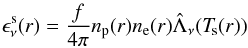 with
with 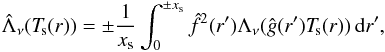
where np(r) and ne(r) are the smooth-flow number densities of the ions and electrons, and r is the radial location of the shock front. The plus sign corresponds to forward and the minus sign to reverse shocks, r′ is the cooling length coordinate with a maximum value of xs, and  and ĝ(r′) denote the normalized density and temperature structures with respect to the shock front (cf. Pauldrach et al. 2001).
As is customary, we list the frequency-integrated X-ray luminosity LX normalized to the bolometric luminosity Lbol; this gives the fraction of the total luminosity emitted in the X-ray regime. We note that most of the locally produced X-ray radiation is reabsorbed by the wind, but a small fraction escapes and is observable as soft X-rays with LX/Lbol ≈ 10-7. Apart from the predicted influence on lines formed within the wind, the accuracy of the shock description can thus be additionally verified by a comparison to direct X-ray observations.
The maximum local shock temperatures Ts(r) are given by the Rankine-Hugoniot relation as function of the immediate jump velocities vs(r). Normalized to the turbulent velocity vt, which can be determined from the fit of the shape of the P-Cygni line profiles, the local values of the jump velocity vs(r) can be estimated via a correlation of vs(r) /vt to the wind outflow velocity v(r) /v∞ (Pauldrach et al. 1994b).
Without a description of clumping based on first principles, clumping is not a single fit factor but a whole number of them, one for each depth point of the model, and thus the degree of freedom is very large.
We had already shown in Kaschinski et al. (2012) that the photospheric absorption lines, which are formed deep in the atmosphere where the density approaches a hydrostatic structure and is therefore independent of the density law used to describe the wind in the outer atmospheric regions, are very similar between fastwind and WM-basic. We therefore refrain from showing those profiles here again and instead remark only that they are also very similar for the benchmark models presented here.
If we knew that the winds were completely smooth, a point could be made for “empirically” determining the velocity law by trying different parameter values in the prescription and choosing the one that leads to the best fit of the Hα line profile, but once we admit clumping, for which we have no theory to predict the radial run either, such reasoning becomes rather specious.
Under certain conditions a sub-Chandrasekhar-mass progenitor may also explode as a supernova, see, e.g., Janka (2011). Furthermore, since we find CSPNs close to the Chandrasekhar limit, we can speculate as to whether these results may be extrapolated to suggest the existence of CSPNs whose combined core-plus-envelope mass perhaps exceeds the Chandrasekhar limit, so that burning of the envelope might cause the core to grow in mass and become critical – cf. Pauldrach (2010).
Acknowledgments
We thank Joachim Puls for his advice and for the fastwind comparison models; Rolf Kudritzki for making the optical observations available to us; and Miguel Urbaneja for sharing his original CSPN model runs. We also thank the anonymous referees for helpful comments which improved the paper. This work was supported by the Deutsche Forschungsgemeinschaft (DFG) under grants Pa 477/4-1 and Pa 477/7-1.
References
- Chandrasekhar, S. 1931, ApJ, 74, 81 [NASA ADS] [CrossRef] [Google Scholar]
- Ebbets, D. C., & Savage, B. D. 1982, ApJ, 262, 234 [NASA ADS] [CrossRef] [Google Scholar]
- Guerrero, M. A. 2006, in Planetary Nebulae in our Galaxy and Beyond, eds. M. J. Barlow, & R. H. Méndez, IAU Symp., 234, 153 [Google Scholar]
- Guerrero, M. A., Chu, Y.-H., & Gruendl, R. A. 2000, ApJS, 129, 295 [NASA ADS] [CrossRef] [Google Scholar]
- Guerrero, M. A., Chu, Y.-H., Gruendl, R. A., & Meixner, M. 2005, A&A, 430, L69 [NASA ADS] [CrossRef] [EDP Sciences] [Google Scholar]
- Herald, J. E., & Bianchi, L. 2011, MNRAS, 417, 2440 [NASA ADS] [CrossRef] [Google Scholar]
- Hoffmann, T. L., & Pauldrach, A. W. A. 2003, in Planetary Nebulae: Their Evolution and Role in the Universe, eds. S. Kwok, M. Dopita, & R. Sutherland, IAU Symp., 209, 189 [Google Scholar]
- Janka, H. T. 2011, in Supernovae und kosmische Gammablitze (Heidelberg: Springer-Verlag), 180 [Google Scholar]
- Kaschinski, C. B., Pauldrach, A. W. A., & Hoffmann, T. L. 2012, A&A, 542, A45 [NASA ADS] [CrossRef] [EDP Sciences] [Google Scholar]
- Kastner, J. H., Montez, Jr., R.,Balick, B., et al. 2012, AJ, 144, 58 [NASA ADS] [CrossRef] [EDP Sciences] [Google Scholar]
- Kudritzki, R. P., Méndez, R. H., Puls, J., & McCarthy, J. K. 1997, in Planetary Nebulae, eds. H. J. Habing, & H. J. G. L. M. Lamers, IAU Symp., 180, 64 [Google Scholar]
- Kudritzki, R. P., Urbaneja, M. A., & Puls, J. 2006, in Planetary Nebulae in our Galaxy and Beyond, eds. M. J. Barlow, & R. H. Méndez, IAU Symp., 234, 119 [Google Scholar]
- Li, W., Bloom, J. S., Podsiadlowski, P., et al. 2011, Nature, 480, 348 [NASA ADS] [CrossRef] [Google Scholar]
- Lucy, L. B. 1982, ApJ, 255, 286 [NASA ADS] [CrossRef] [Google Scholar]
- Lucy, L. B., & Solomon, P. M. 1970, ApJ, 159, 879 [NASA ADS] [CrossRef] [Google Scholar]
- Lucy, L. B., & White, R. L. 1980, ApJ, 241, 300 [NASA ADS] [CrossRef] [Google Scholar]
- Méndez, R. H., Kudritzki, R. P., Groth, H. G., Husfeld, D., & Herrero, A. 1988a, A&A, 197, L25 [NASA ADS] [Google Scholar]
- Méndez, R. H., Kudritzki, R. P., Herrero, A., Husfeld, D., & Groth, H. G. 1988b, A&A, 190, 113 [NASA ADS] [Google Scholar]
- Milne, E. A. 1926, MNRAS, 86, 459 [NASA ADS] [Google Scholar]
- Morton, D. C. 1991, ApJS, 77, 119 [NASA ADS] [CrossRef] [Google Scholar]
- Owocki, S. P., & Rybicki, G. B. 1984, ApJ, 284, 337 [NASA ADS] [CrossRef] [Google Scholar]
- Pauldrach, A. 1987, A&A, 183, 295 [NASA ADS] [Google Scholar]
- Pauldrach, A. W. A. 2010, in Dunkle kosmische Energie (Heidelberg: Springer-Verlag), 304 [Google Scholar]
- Pauldrach, A. W. A., & Puls, J. 1990a, Rev. Mod. Astron., 3, 124 [Google Scholar]
- Pauldrach, A. W. A., & Puls, J. 1990b, A&A, 237, 409 [NASA ADS] [Google Scholar]
- Pauldrach, A., Puls, J., & Kudritzki, R. P. 1986, A&A, 164, 86 [NASA ADS] [Google Scholar]
- Pauldrach, A., Puls, J., Kudritzki, R. P., Méndez, R. H., & Heap, S. R. 1988, A&A, 207, 123 [NASA ADS] [Google Scholar]
- Pauldrach, A. W. A., Kudritzki, R. P., Puls, J., & Butler, K. 1990a, A&A, 228, 125 [NASA ADS] [Google Scholar]
- Pauldrach, A. W. A., Puls, J., Gabler, R., & Gabler, A. 1990b, in Properties of Hot Luminous Stars, ed. C. D. Garmany, ASP Conf. Ser., 7, 171 [NASA ADS] [Google Scholar]
- Pauldrach, A. W. A., Feldmeier, A., Puls, J., & Kudritzki, R. P. 1994a, in Evolution of Massive Stars, eds. D. Vanbeveren, W. van Rensbergen, & C. De Loore, 105 [Google Scholar]
- Pauldrach, A. W. A., Kudritzki, R. P., Puls, J., Butler, K., & Hunsinger, J. 1994b, A&A, 283, 525 [Google Scholar]
- Pauldrach, A. W. A., Hoffmann, T. L., & Lennon, M. 2001, A&A, 375, 161 [NASA ADS] [CrossRef] [EDP Sciences] [Google Scholar]
- Pauldrach, A. W. A., Hoffmann, T. L., & Méndez, R. H. 2003, in Planetary Nebulae: Their Evolution and Role in the Universe, eds. S. Kwok, M. Dopita, & R. Sutherland, IAU Symp., 209, 177 [Google Scholar]
- Pauldrach, A. W. A., Hoffmann, T. L., & Méndez, R. H. 2004, A&A, 419, 1111 [NASA ADS] [CrossRef] [EDP Sciences] [Google Scholar]
- Pauldrach, A. W. A., Vanbeveren, D., & Hoffmann, T. L. 2012, A&A, 538, A75 [NASA ADS] [CrossRef] [EDP Sciences] [Google Scholar]
- Puls, J., & Hummer, D. G. 1988, A&A, 191, 87 [NASA ADS] [Google Scholar]
- Puls, J., & Pauldrach, A. W. A. 1991, in NATO Advanced Science Institutes (ASI) Series C, Vol. 341, eds. L. Crivellari, I. Hubeny, & D. G. Hummer, 175 [Google Scholar]
- Puls, J., Urbaneja, M. A., Venero, R., et al. 2005, A&A, 435, 669 [NASA ADS] [CrossRef] [EDP Sciences] [Google Scholar]
- Puls, J., Markova, N., Scuderi, S., et al. 2006, A&A, 454, 625 [NASA ADS] [CrossRef] [EDP Sciences] [Google Scholar]
- Repolust, T., Puls, J., & Herrero, A. 2004, A&A, 415, 349 [NASA ADS] [CrossRef] [EDP Sciences] [Google Scholar]
- Roelofs, G., Bassa, C., Voss, R., & Nelemans, G. 2008, MNRAS, 391, 290 [NASA ADS] [CrossRef] [Google Scholar]
- Sana, H., Rauw, G., & Gosset, E. 2005, in Massive Stars and High-Energy Emission in OB Associations, eds. G. Rauw, Y. Nazé, R. Blomme, & E. Gosset, 107 [Google Scholar]
- Sana, H., Rauw, G., Nazé, Y., Gosset, E., & Vreux, J.-M. 2006, MNRAS, 372, 661 [NASA ADS] [CrossRef] [Google Scholar]
- Schaefer, B. E., & Pagnotta, A. 2012, Nature, 481, 164 [NASA ADS] [CrossRef] [Google Scholar]
- Snow, Jr., T. P., & Morton, D. C. 1976, ApJS, 32, 429 [NASA ADS] [CrossRef] [Google Scholar]
- Stoner, E. C. 1930, Phil. Mag., 9, 944 [CrossRef] [Google Scholar]
- Taresch, G., Kudritzki, R. P., Hurwitz, M., et al. 1997, A&A, 321, 531 [NASA ADS] [Google Scholar]
Appendix A: Additional material
Shock structures in the winds of the central stars of NGC 2392, IC 4593, IC 418, and NGC 6826, determined from fits of the calculated O vi lines to the FUSE observations.
 |
Fig. A.1 Synthetic UV spectra (black) from consistent models for NGC 2392, compared to the observed UV spectra (red and blue). The top panel show the spectrum from a model using the stellar parameters from the analysis of K06. The spectrum is clearly incompatible with the observations, thus ruling out this parameter set. The center panel shows the spectrum from a model using the parameters from the analysis of P04. The spectrum predicted by the model is generally in good agreement with the observations, but the O vi line is not reproduced. In the bottom panel, shocks in the wind have additionally been included in the modeling procedure. The small amount of high-energy radiation (LX/Lbol ~ 10-6) generated by these shocks is enough to ionize a small fraction of oxygen into O vi, sufficient to reproduce the observed line strength. This result indicates strongly that shocks and the X-ray radiation emitted by them play a role not only in the winds of massive O stars, but also in the winds of O-type CSPNs. |
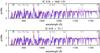 |
Fig. A.5 Observed FUSE spectrum of IC 418 (red), compared to the observed spectra of He 2-131 (blue, upper panel) and Tc 1 (blue, lower panel). The comparison shows that the O vi line in the spectra of Tc 1 and He 2-131 is very similar to that of IC 418 despite differences in the terminal velocity. |
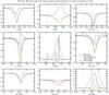 |
Fig. A.6 Observed optical line profiles of NGC 2392 (black) compared to predicted line profiles from four different models. Colors indicate different stellar and wind parameter sets, while dash styles indicate different clumping factors. The colors correspond to: the consistent model of P04 (P04, red); a model using the stellar parameters of K06 with mass loss rate and terminal velocity artificially set to the values given by K06 (K06f, green); and one using the stellar parameters of K06 and wind parameters consistent with those stellar parameters (K06c, blue). Solid lines indicate models using the clumping factor suggested by K06, the dash-dotted line indicates a model using the clumping factor redetermined in this work. |
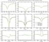 |
Fig. A.8 As Fig. A.7, but for NGC 3242. This is the only CSPN for which the consistent wind calculation yields the same mass loss rate and terminal velocity as the optical analysis by K06 and the “green” model is thus identical to the “blue” one (which is therefore not shown). |
 |
Fig. A.15 Synthetic UV spectra of NGC 6826 (upper two panels) and IC 418 (lower two panels) calculated with the stellar parameters determined by the UV analysis, compared to the observed UV spectra. The first panels in the upper and lower part show unclumped models. The overall fit to the observed UV spectra is generally very good, although the He iiλ 1640 line is not reproduced too well. The second panels in the upper and lower parts show the same models, but with a clumping factor of fcl = 4. Most of the UV spectrum is not affected, except for a few lines from subordinate ionization stages (such as P vλ 1118, C iiiλ 977, and H iλ 1216). In particular the match to the observed He iiλ 1640 line is now almost excellent. |
All Tables
Stellar masses and wind parameters for the six selected stars of our sample of CSPNs for which FUSE observations are available.
Shock structures in the winds of the central stars of NGC 2392, IC 4593, IC 418, and NGC 6826, determined from fits of the calculated O vi lines to the FUSE observations.
All Figures
|
Fig. 1 Observed UV and optical spectrum of IC 4593 (gray) compared to synthetic spectra computed from atmospheric models with consistently calculated winds, based on the stellar parameter sets of Kudritzki et al. 2006 (K06c; blue) and Pauldrach et al. 2004 (P04; red). The K06c spectrum shows large differences to the observed spectrum, thus arguing against this parameter set, whereas the P04 spectrum is in generally much better agreement with the observed spectrum. (For cosmetic reasons, and to identify and distinguish the interstellar lines from the stellar features, the most important interstellar lines (primarily absorption by molecular and atomic hydrogen) have also been included in the latter model12.) The plot also illustrates the well-known fact that the UV spectrum of O stars contains much more, and stronger, spectral lines than the optical. Given the furthermore known sensitivity of the optical emission lines to physical and modeling uncertainties such as clumping (to which the UV spectrum is much more robust), this emphasizes that the UV carries much more diagnostic weight than the optical. |
| In the text | |
|
Fig. 2 Excerpt of Fig. 5 of Pauldrach et al. (2012) showing the appearance of the visible UV spectrum of massive O stars as a function of mass M for a constant effective temperature Teff and radius R, resulting from dynamically consistent wind models. (Teff = 40 000 K, R = 15 R⊙, and solar abundances have been assumed for the models.) Although the mass of the first model is only 20% smaller than that of the second one, the resulting UV spectra appear markedly different. Because of this strong response, the UV spectrum can be used diagnostically for a determination of the stellar mass. A corresponding dependence of the appearance of the UV spectrum on the stellar parameters as shown here for massive O stars also holds for O-type CSPNs, which have comparable wind densities and velocities (see text), and thus similar UV spectra. |
| In the text | |
|
Fig. 3 Appearance of the UV spectrum for two dynamically consistent CSPN models with different stellar parameters (as labeled), illustrating the strong reaction of the UV spectrum to changes in the stellar parameters. Because of this sensitive dependence, the UV spectrum can be used diagnostically for a fine-grained determination of the stellar parameters, in particular the masses. |
| In the text | |
|
Fig. 4 Comparison of Hα line profiles predicted by fastwind (red) and WM-basic (black). To focus the comparison on the NLTE modeling and the treatment of radiative transfer, these WM-basic calculations use the density structures from the fastwind models. Top row: Teff = 50 000 K test model (S50), bottom row: Teff = 35 000 K test model (S35). Left panels: profiles from a smooth, unclumped flow (fcl = 1), right panels: profiles from a clumped flow (fcl = 81) with a correspondingly reduced mass loss rate (by a factor of |
| In the text | |
|
Fig. 5 Hα line profile of the S35 test model as in Fig. 4, but this time also showing the case of a clumped wind (fcl = 81, as in Fig. 4) with the “normal” mass loss rate (blue). Compared to this strong response, the small differences between two corresponding fastwind (red) and WM-basic (black solid line) predictions are insignificant. |
| In the text | |
|
Fig. A.1 Synthetic UV spectra (black) from consistent models for NGC 2392, compared to the observed UV spectra (red and blue). The top panel show the spectrum from a model using the stellar parameters from the analysis of K06. The spectrum is clearly incompatible with the observations, thus ruling out this parameter set. The center panel shows the spectrum from a model using the parameters from the analysis of P04. The spectrum predicted by the model is generally in good agreement with the observations, but the O vi line is not reproduced. In the bottom panel, shocks in the wind have additionally been included in the modeling procedure. The small amount of high-energy radiation (LX/Lbol ~ 10-6) generated by these shocks is enough to ionize a small fraction of oxygen into O vi, sufficient to reproduce the observed line strength. This result indicates strongly that shocks and the X-ray radiation emitted by them play a role not only in the winds of massive O stars, but also in the winds of O-type CSPNs. |
| In the text | |
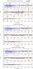 |
Fig. A.2 As Fig. A.1, but for IC 4593. |
| In the text | |
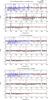 |
Fig. A.3 As Fig. A.1, but for IC 418. |
| In the text | |
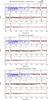 |
Fig. A.4 As Fig. A.1, but for NGC 6826. |
| In the text | |
|
Fig. A.5 Observed FUSE spectrum of IC 418 (red), compared to the observed spectra of He 2-131 (blue, upper panel) and Tc 1 (blue, lower panel). The comparison shows that the O vi line in the spectra of Tc 1 and He 2-131 is very similar to that of IC 418 despite differences in the terminal velocity. |
| In the text | |
|
Fig. A.6 Observed optical line profiles of NGC 2392 (black) compared to predicted line profiles from four different models. Colors indicate different stellar and wind parameter sets, while dash styles indicate different clumping factors. The colors correspond to: the consistent model of P04 (P04, red); a model using the stellar parameters of K06 with mass loss rate and terminal velocity artificially set to the values given by K06 (K06f, green); and one using the stellar parameters of K06 and wind parameters consistent with those stellar parameters (K06c, blue). Solid lines indicate models using the clumping factor suggested by K06, the dash-dotted line indicates a model using the clumping factor redetermined in this work. |
| In the text | |
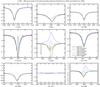 |
Fig. A.7 As Fig. A.6, but for IC 4637. Profiles from unclumped models are additionally shown dashed. |
| In the text | |
|
Fig. A.8 As Fig. A.7, but for NGC 3242. This is the only CSPN for which the consistent wind calculation yields the same mass loss rate and terminal velocity as the optical analysis by K06 and the “green” model is thus identical to the “blue” one (which is therefore not shown). |
| In the text | |
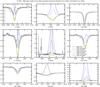 |
Fig. A.9 As Fig. A.7, but for IC 4593. |
| In the text | |
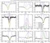 |
Fig. A.10 As Fig. A.7, but for IC 418. |
| In the text | |
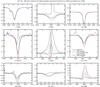 |
Fig. A.11 As Fig. A.6, but for He 2-108. |
| In the text | |
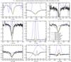 |
Fig. A.12 As Fig. A.7, but for Tc 1. |
| In the text | |
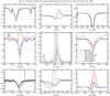 |
Fig. A.13 As Fig. A.7, but for He 2-131. |
| In the text | |
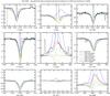 |
Fig. A.14 As Fig. A.7, but for NGC 6826. |
| In the text | |
|
Fig. A.15 Synthetic UV spectra of NGC 6826 (upper two panels) and IC 418 (lower two panels) calculated with the stellar parameters determined by the UV analysis, compared to the observed UV spectra. The first panels in the upper and lower part show unclumped models. The overall fit to the observed UV spectra is generally very good, although the He iiλ 1640 line is not reproduced too well. The second panels in the upper and lower parts show the same models, but with a clumping factor of fcl = 4. Most of the UV spectrum is not affected, except for a few lines from subordinate ionization stages (such as P vλ 1118, C iiiλ 977, and H iλ 1216). In particular the match to the observed He iiλ 1640 line is now almost excellent. |
| In the text | |
Current usage metrics show cumulative count of Article Views (full-text article views including HTML views, PDF and ePub downloads, according to the available data) and Abstracts Views on Vision4Press platform.
Data correspond to usage on the plateform after 2015. The current usage metrics is available 48-96 hours after online publication and is updated daily on week days.
Initial download of the metrics may take a while.