| Issue |
A&A
Volume 591, July 2016
|
|
|---|---|---|
| Article Number | A146 | |
| Number of page(s) | 17 | |
| Section | Planets and planetary systems | |
| DOI | https://doi.org/10.1051/0004-6361/201628331 | |
| Published online | 01 July 2016 | |
The SOPHIE search for northern extrasolar planets
XI. Three new companions and an orbit update: Giant planets in the habitable zone⋆
1 Observatoire Astronomique de
l’Université de Genève, 51 Chemin
des Maillettes, 1290
Versoix,
Switzerland
e-mail: This email address is being protected from spambots. You need JavaScript enabled to view it.
2 Aix Marseille Université, CNRS, LAM
(Laboratoire d’Astrophysique de Marseille) UMR 7326, 13388
Marseille,
France
3 Institut d’Astrophysique de Paris,
UMR 7095 CNRS, Université Pierre & Marie Curie, 98bis boulevard Arago, 75014
Paris,
France
4 Observatoire de Haute Provence, CNRS,
Aix Marseille Université, Institut Pythéas UMS 3470, 04870 Saint-Michel-l’ Observatoire,
France
5 Université Grenoble Alpes,
IPAG,
38000
Grenoble,
France
6 CNRS, IPAG, 38000
Grenoble,
France
7 Canada-France-Hawaii Telescope
Corporation, 65-1238 Mamalahoa Hwy, Kamuela, HI
96743,
USA
8 Cavendish Laboratory,
J J Thomson Avenue,
Cambridge
CB3 0HE,
UK
9 Instituto de Astrofísica e Ciências
do Espaço, Universidade do Porto, CAUP, Rua das Estrelas, 4150-762
Porto,
Portugal
10 Departamento de Física e
Astronomia, Faculdade de Ciências, Universidade do Porto, Rua do Campo Alegre, 4169-007
Porto,
Portugal
11 European Space Agency, European
Space Astronomy Centre, PO Box 78, Villanueva de la Canada,
28691
Madrid,
Spain
Received:
17
February
2016
Accepted:
12
April
2016
Abstract
We report the discovery of three new substellar companions to solar-type stars, HD 191806, HD 214823, and HD 221585, based on radial velocity measurements obtained at the Haute-Provence Observatory. Data from the SOPHIE spectrograph are combined with observations acquired with its predecessor, ELODIE, to detect and characterise the orbital parameters of three new gaseous giant and brown dwarf candidates. Additionally, we combine SOPHIE data with velocities obtained at the Lick Observatory to improve the parameters of an already known giant planet companion, HD 16175 b. Thanks to the use of different instruments, the data sets of all four targets span more than ten years. Zero-point offsets between instruments are dealt with using Bayesian priors to incorporate the information we possess on the SOPHIE/ELODIE offset based on previous studies. The reported companions have orbital periods between three and five years and minimum masses between 1.6 MJup and 19 MJup. Additionally, we find that the star HD 191806 is experiencing a secular acceleration of over 11 m s-1 per year, potentially due to an additional stellar or substellar companion. A search for the astrometric signature of these companions was carried out using Hipparcos data. No orbit was detected, but a significant upper limit to the companion mass can be set for HD 221585, whose companion must be substellar. With the exception of HD 191806 b, the companions are located within the habitable zone of their host star. Therefore, satellites orbiting these objects could be a propitious place for life to develop.
Key words: planetary systems / techniques: radial velocities / stars: individual: HD 221585 / stars: individual: HD 16175 / stars: individual: HD 191806 / stars: individual: HD 214823
Based on observations collected with the SOPHIE spectrograph on the 1.93-m telescope at Observatoire de Haute-Provence (CNRS), France by the SOPHIE Consortium (programme 07A.PNP.CONS to 15A.PNP.CONS).
© ESO, 2016
1. Introduction
As the baselines of radial velocity surveys move from years to decades, it becomes possible to probe regions progressively farther away from the targeted stars. With over 20 years of radial velocity observations under the belt, this has in fact already been achieved for giant planets. As of December 2015, the exoplanets.org database (Han et al. 2014) listed over a hundred planets detected with semi-major axes larger than 2 au. Most of these orbit solar-type stars and, with two notable exceptions, namely HD 10180 h (Lovis et al. 2011b) and HD 204941 b (Dumusque et al. 2011), all of these planets have masses larger than Saturn.
The discovery of giant planetary companions on long-period orbits is important for a number of reasons: firstly, probing the architecture of extrasolar systems out to the ice line and beyond provides strong constraints on planet formation and evolution. Secondly, it allows us to put our own solar system in context. Thirdly, these giant planets are likely to play an important role in the short-term dynamics of the systems. For example, an unseen massive companion in an outer orbit can bias the mass determinations obtained via transit timing variations of small-mass planets in close-in compact systems, the likes of which have been abundantly discovered by the Kepler mission (e.g. Rowe et al. 2014). Finally, the discovery of these companions is important on account of the role of Jupiter in the impact rate on Earth of asteroids and comets, and the consequent effect on habitability (see Laakso et al. 2006; Horner & Jones 2008, 2010, and references therein). Additionally, although gaseous planets are most likely incapable of harbouring life, they could be orbited by rocky satellites that are analogous to the Galilean satellites of Jupiter or larger. If the giant planet orbits in the habitable zone of its star, these moons would constitute a suitable place for life to develop (Williams et al. 1997; Porter & Grundy 2011; Heller et al. 2014; Heller & Pudritz 2015). Therefore, establishing whether a gaseous planet is in the habitable zone (Kasting et al. 1993; Kopparapu et al. 2013b) bears importance for future astrobiological studies.
Two factors act as the main limitation to the endeavour of unveiling such planets. Firstly, no single unmodified RV instrument has observed uninterrupted for 20 years; ELODIE (Baranne et al. 1996) was replaced with SOPHIE in 2006 (Perruchot et al. 2008; Bouchy et al. 2009a). In turn SOPHIE was upgraded in 2011 (Bouchy et al. 2013; Perruchot et al. 2011). The HIRES instrument was upgraded in 2004 (Vogt et al. 1994), and CORALIE was upgraded in 2007 and 2014 (Queloz et al. 2000; Ségransan et al. 2010). The planet search programme at the 2.4-m telescope of the McDonald Observatory went through three instrumental phases, the latter of which started in 1998 (Hatzes et al. 2000; Endl et al. 2004). Even HARPS, which remained untouched for over ten years, has recently been upgraded (Mayor et al. 2003; Lo Curto et al. 2015). This implies that instrument offsets have to be treated cautiously to avoid introducing spurious signals that pass for long-period giant planets. This is particularly important when no overlap between the instruments exist, as is the case for most of the examples cited above.
Secondly, many solar-type stars, even the most inactive, exhibit activity cycles or variations with typical timescales between a few years and a couple of decades (Baliunas et al. 1995; Lovis et al. 2011a). Long-term activity variations are related to global changes in the convective pattern of the star (Lindegren & Dravins 2003; Meunier et al. 2010; Meunier & Lagrange 2013), and produce radial velocity signals clearly correlated with activity proxies such as  (Noyes et al. 1984) and the width and asymmetry of the mean spectral line (Dravins 1982; Santos et al. 2010; Lovis et al. 2011a; Dumusque et al. 2011; Díaz et al. 2016). These signals can be mistaken with long-period planets, and if not fully corrected, can contaminate the radial velocity time series at higher frequencies.
In this article, we tackle these issues by modelling radial velocity time series using a Bayesian approach. Information such as the calibrations of instrument offsets are incorporated into the model through the use of Bayesian priors. We report the detection of three new long-period giant companions around solar-type stars based on data obtained with the ELODIE and SOPHIE spectrographs. One of these companions has a minimum mass of around 19 MJup and may in fact be a brown dwarf. Additionally, we improved upon the orbital and physical parameters of a known giant planet candidate by combining the original discovery data with new measurements from ELODIE and SOPHIE. The paper is organised as follows: in Sect. 2 we describe the observations and the techniques used to reduce the data. Section 3 describes the stellar hosts, their basic physical properties and their activity level over the time span of our observations. We discuss the presence of activity cycles here. Section 4 presents the results of the analysis of the bisector of the stellar mean line, and in Sect. 5 we describe our model and the technique to sample the posterior distribution of the model parameters. The results are presented individually for each target in Sect. 6. We study the position of the candidates with respect to the habitable zone and the habitability of potential satellites in Sect. 7 and, finally, we give a summary of the results in Sect. 8.
2. Observations and data reduction
Basic characteristics of the ELODIE, SOPHIE, and SOPHIE+ observations of the four target stars.
The targets were observed as part of the volume-limited SOPHIE survey for giant planets (sub-programme 2, or SP2; Bouchy et al. 2009a). SOPHIE is a fibre-fed, cross-dispersed echelle spectrograph mounted at the 1.93-m telescope of the Haute-Provence Observatory. Its dispersive elements are kept at constant pressure and it is installed in a temperature stabilised environment (Perruchot et al. 2008) to provide high-precision radial velocity measurements over long timescales. Observations of SP2 targets are carried out in the high-resolution mode of the instrument, which provides resolving power R = 75 000. In addition to the target fibre, a second fibre monitors sky brightness variations, particularly because of the scattered moonlight.
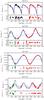 |
Fig. 1 Radial velocity data and model fits. The green points represent ELODIE data, and the red empty and filled circles represent SOPHIE and SOPHIE+ data, respectively. The empty black points are Lick Observatory data. In the upper panel of each plot, the solid thick black curve is the maximum a posteriori physical model. The blue curves are the 95% highest density interval (HDI) for the complete model, computed as described in Díaz et al. (2016) and Gregory (2011). The model posterior mean is represented by solid thin grey curve. The stellar drift or systemic velocity is shown as a thick grey line with the 95% (HDI) shown with dotted grey lines. |
Sub-programme 2, targets 2300 dwarf stars at distance <60 pc and with B − V between 0.35 and 1.0. Most of these stars (about 1900) have already been observed with SOPHIE (Hébrard et al. 2016). The programme employs medium-precision measurements (around 3 m/s) that permitted the detection of around 50 substellar companions, including giant planets in multi-planetary systems (e.g. Hébrard et al. 2010; Moutou et al. 2014) and brown dwarf companions (Díaz et al. 2012; Wilson et al. 2016). The observing strategy consists in acquiring spectra with a constant signal-to-noise ratio (S/N) of around 50 to minimise the effects of the charge transfer inefficiency (Bouchy et al. 2009b). This is usually achieved in a few minutes of integration time, but as the SP2 is also used as a backup programme for the SOPHIE programmes that require more precise measurements, some exposures during poor weather conditions are much longer.
The spectra were reduced using the SOPHIE pipeline described by Bouchy et al. (2009a). The radial velocity (RV) was measured by weighted cross correlation of the extracted two-dimensional echelle spectra with a spectral mask corresponding to the spectral type of the observed star (Baranne et al. 1996; Pepe et al. 2002). A Gaussian curve was fitted to the cross-correlation function (CCF) averaged over all spectral orders to produce the RV measurement. Additionally, we obtained the bisector velocity span of the CCF as described by Queloz et al. (2001). The measurements are listed in Tables B.1 through B.41.
One of the main systematic effects in SOPHIE data was due to insufficient scrambling of the fibre link and the high sensitivity of the spectrograph to illumination variations. As a consequence, seeing changes at the fibre input produced changes in the measured radial velocity. This so-called seeing effect is described in Boisse et al. (2010, 2011a), Díaz et al. (2012), and Bouchy et al. (2013). The seeing effect can be partially corrected for by measuring the RV on each half of spectral orders and using the difference of the obtained velocities to decorrelate the velocity measured with the entire detector (see Bouchy et al. 2013). This correction was applied to all data obtained with SOPHIE before June 2011. The seeing effect was dramatically reduced in June 2011 (BJD = 2 455 730) with the introduction of octagonal-section fibres in the fibre link. The new fibre may have caused a zero-point shift, which is not yet fully characterised. In this article, we treat SOPHIE data obtained after June 2011 as if it were from a different instrument, which we refer to as SOPHIE+. In spite of an important improvement in the SOPHIE RV precision, some systematic zero-point offsets are still observed. They are probably related to an incomplete thermal isolation and are corrected for as described by Courcol et al. (2015).
All of the targets were already observed with the ELODIE spectrograph (Baranne et al. 1996), which is the predecessor of SOPHIE. However, they were not included in SOPHIE sub-programme 5, which follows up velocity trends and incomplete orbits identified with ELODIE (Bouchy et al. 2009a, 2016; Boisse et al. 2012). The ELODIE RVs were also obtained by cross correlation with a numerical spectral mask. A velocity offset between ELODIE and SOPHIE exists and has been calibrated by Boisse et al. (2012) as a function of colour index B − V using a sample of around 200 stars. These authors mentioned that a dependence on stellar metallicity must exist, but they claimed the effect is small and decided to neglect it.
Table 1 lists the main characteristics of the ELODIE, SOPHIE, and SOPHIE+ data sets. The data sets are plotted in Fig. 1. In all cases, clear RV variations exist, which are due to substellar orbiting companions, as we show below. The measured orbital and physical parameters are listed in Table 4.
3. Stellar parameters
The atmospheric parameters (stellar effective temperature Teff, surface gravity log (g), and metallicity [Fe/H]) of the four observed targets were computed from the combined SOPHIE spectra. The method is described in Santos et al. (2004) and Sousa et al. (2008). Stellar masses M⋆ are then derived from the calibration of Torres et al. (2010) with a correction following Santos et al. (2013). Errors were computed from 10 000 random draws from the posterior distribution of the stellar parameters, assumed Gaussian, and free of correlations. The stellar ages are derived by interpolation of the PARSEC (Bressan et al. 2012) tracks as described by da Silva et al. (2006). The obtained parameters are listed in Table 2. The statistical uncertainty in the stellar masses obtained by this method is known to be underestimated. Instead, we used a conservative 10% error in all computations requiring the stellar mass, such as the minimum masses of the companions. For HD 16175, a number of determinations of the stellar parameters exist in the literature (Peek et al. 2009; Santos et al. 2013; Sousa et al. 2015; Jofré et al. 2015). They all agree within the error bars. We decided to retain the determination by Sousa et al. (2015) because they used the same method that we employed for the remaining stars.
Using the Hipparcos parallaxes, and the measured apparent magnitudes, we obtained the absolute magnitudes in the V band, MV. With these absolute magnitudes, along with the bolometric correction tabulated by Cox (2000) and the self-consistent value adopted for the absolute bolometric magnitude of the Sun, Mbol, ⊙ = 4.61 (Torres 2010), we can compute the stellar luminosity in solar units. The obtained values are listed in Table 2, and the uncertainties are propagated assuming a negligible error for the bolometric correction. In Fig. 2 the position of the target stars in the effective temperature – luminosity plane is compared with the PARSEC theoretical tracks (Bressan et al. 2012). We notice that all stars have evolved away from the zero-age main sequence, which is represented by the bottom points of each track. The most evolved star is HD 221585, whose age is estimated at 6.2 ± 0.5 Gyr. The remaining stars are around 3 Gyr in age. Their evolution can be quantified using the evolution metric from Wright (2005), ΔMV, which measures the magnitude difference in the V band between the star and the main sequence. This metric is given in Table 2 and confirms that HD 221585 is the most evolved star in our sample, followed by HD 214823. Also, the stellar masses estimated using the Torres et al. (2010) calibration do not generally agree with those that would have been obtained from interpolating the PARSEC tracks. This justifies the use of a 10% error in the stellar masses for the computation of the derived quantities. A similar discrepancy is seen for the ages of the stars, also hinting at a systematic uncertainty unaccounted for in the error bars listed in Table 2.
Finally, we used the SOPHIE CCF to estimate the projected stellar rotational velocities, vsinI∗, using the calibration by Boisse et al. (2010). The value of the projected rotational velocity of the star determined spectroscopically by Peek et al. (2009) for HD 16175, vsinI∗ = 4.8 ± 0.5 km s-1 , is in agreement with the value obtained from the SOPHIE CCF.
3.1. Activity indexes
The classical activity index, based on the Ca II H and K lines, , cannot be obtained from the ELODIE spectra because the H and K lines are not included in the wavelength range. Also the proxy is not easily exploitable from the SOPHIE spectra of these targets due to a poor instrumental response and typically low flux level in this region of the stellar spectrum. As a consequence, the SOPHIE time series are usually very noisy. In contrast, the average is probably a good indicator of the mean activity level of the star and, therefore, of the expected RV jitter (e.g. Santos et al. 2000; Wright 2005) and stellar rotational period (Mamajek & Hillenbrand 2008). The RV jitter level estimated using the prescription of Wright (2005) is expected to be of a few m s-1, which is comparable with the photon noise error listed in Table 1. The estimated rotational periods are listed in Table 2, where the error bars correspond to the dispersion originated in the measurements. As expected, stars showing a higher mean value of (HD 16175 and HD 214823) also present higher rotational velocities.
The Hα line is formed at a lower altitude in the stellar atmosphere than the Ca II H and K lines, but it was shown to be a good chromospheric indicator (e.g. Mauas & Falchi 1994) and is used frequently (e.g. Pasquini & Pallavicini 1991; Montes et al. 1995; Cincunegui et al. 2007b,a; Robertson et al. 2013, 2014; Neveu-VanMalle et al. 2016). Furthermore, at the spectral location of the Hα line SOPHIE and ELODIE have a much higher instrumental response and, therefore, the activity index based on the Hα transition line can be readily computed. The activity index is defined as the ratio between the flux in the Hα line and a reference flux near the continuum level. We chose a 10.76 Å window centred at 6550 Å and a 8.75 Å window centred at 6580 Å for the reference windows. We used 0.68 Å window centred at 6562.808 Å2 for the line flux measurement. The Hα activity index cannot be used to compare the activity level of different stars, since the flux ratio used in its definition depends not only on activity level, but also on the spectral type of each star. The index can be corrected as carried out by Cincunegui et al. (2007b) by subtracting an estimation of the photospheric flux. In the scope of this paper, we are interested exclusively in the relative activity changes of each star and, therefore, we did not correct the Hα index.
Stellar parameters.
The Hα measurements are plotted in the upper row of Fig. 3. The lower row presents the periodogram computed using only the SOPHIE and SOPHIE+ measurements. The ELODIE measurements were excluded from the frequency analysis because an offset is expected between ELODIE and SOPHIE Hα measurements, but has not yet been calibrated. The position of the highest peak in the periodogram is in agreement with the expected stellar rotational period obtained based on the indicator (see Table 2) for HD 214823 and HD 221585. For HD 16175 and HD 191806, power is seen at the expected rotational period (~20 days), but the highest peak is elsewhere. For HD 16175, if we remove the observation with the lowest S/N, 31, compared to the mean of 53, the highest peak shifts to 12.1 days, which is close to the expected rotational period of 19.7 ± 5.5 days.
The periodogram of the Hα time series of HD 191806 shows a prominent peak at around 1600 days, similar to the period of the detected companion. However, the correlation between velocities and Hα measurements is weak (Pearson’s coefficient <0.3), and when a sinusoidal model with this frequency is fit to the Hα data, the amplitude is compatible with zero3. Furthermore, we computed the Bayes factor between this model and a model without variation. Using the estimator of Perrakis et al. (2014) we found that the simpler model is 86.1 ± 0.2 times more probable than the sinusoidal model. In contrast, when the period of the putative signal is allowed to vary, we obtained a Bayes factor of 2.2 ± 0.2 for the sinusoidal model. This is considered mild evidence against the null hypothesis and “not worth more than a bare mention” (Kass & Raftery 1995). We conclude that the peak observed at this frequency is not significant. Therefore, none of the target stars exhibit activity variations with periods larger than ~1000 days. The activity level of HD 214823 seems to be decreasing on a timescale that is much longer than the current time base. Unfortunately, the precision of the measurements is not sufficient to detect a similar variability.
Results of the bisector analysis for SOPHIE and SOPHIE+ data. χ2 statistics under the null hypothesis of no bisector variation.
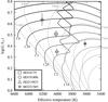 |
Fig. 2 Position of the four target stars in the luminosity-effective temperature plane. The PARSEC theoretical tracks (Bressan et al. 2012) are plotted using shades of grey for different initial stellar masses labelled in solar units at the bottom of each track. The corresponding isochrones are plotted as dotted lines and labelled in light grey. |
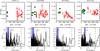 |
Fig. 3 Top row: time series of the Hα activity index. The green points correspond to ELODIE observations, and red empty symbols and red filled symbols are for SOPHIE and SOPHIE+, respectively. The same scale is used for all stars to ease comparison. Bottom row: generalised Lomb-Scargle periodogram for the SOPHIE and SOPHIE+ Hα index. It was assumed that no offset exists between the index measurement of SOPHIE and SOPHIE+. The red vertical dotted lines signal the position of the highest peaks whose periods are annotated, the blue shaded areas represent the 2σ intervals for the stellar rotational periods listed in Table 2, and the green vertical dashed lines corresponds to the maximum a posteriori orbital period of the orbiting companions. |
4. Bisector analysis
The stellar RV signature of a planetary-mass companion can be mimicked by blended stellar systems and nearly face-on stellar binaries (e.g. Santos et al. 2002; Díaz et al. 2012; Wright et al. 2013). However, while the reflex motion produced by a planetary-mass companion induces a shift of the stellar spectral lines without changing their shape, blended stellar systems and unresolved companions induce some level of variation because of the presence of an additional set of lines. This variation is reflected, in principle, in the bisector velocity span (BVS) obtained from the CCF. However, it may be too small to be detected, especially when the star is a slow rotator (see Santerne et al. 2015). Stellar activity is also known to produce variations in the BVS over the timescale of the rotational period of the star (see e.g. Boisse et al. 2011b) and also throughout stellar activity cycles (see e.g. Díaz et al. 2016).
We searched for significant variations in the SOPHIE BVS (Queloz et al. 2001), as well as correlations between the bisector velocity span and RV measurements. The SOPHIE and SOPHIE+ measurements were considered separately, since the instrument upgrade may have induced changes in the instrumental line profile. The results are presented in Table 3, where we list the p-value of the χ2 statistic under the null hypothesis (i.e. no BVS variation) for each star, assuming the photon noise on the BVS is twice that of the RV measurement (Santerne et al. 2015). No p-value is below the customary limit of 0.05. In view of the excessive tendency of p-value analysis to reject the null hypothesis (see e.g. Sellke et al. 2001), we conclude that no significant variation is seen in the bisector time series, and that, therefore, the variations seen in the RV time series are produced by orbiting substellar companions.
5. Data analysis
5.1. The model
The stellar RV data of instrument k ({ vi } with i = 1,...,Nk) were modelled as originating from independent normal distributions with mean f(ti,θ) and standard deviation σ. The mean f(ti,θ) is the physical model for the RV variations at time ti (with parameter vector θ), which we describe below. The variance can be written  , where σi is the internal photon noise and calibration error of the RV measurement at time ti and
  is the additional noise introduced in the model to represent activity jitter and instrument systematics, which could in principle also be a function of time. The term
  depends on the instrument under consideration, hence the index k. The likelihood for this model then is the product over all of the instruments { k } with k = 1,...,Ninst and all velocity measurements for each instrument as follows:
 ![Mathematical equation: \begin{eqnarray} \small \mathcal{L}(\teta) \!=\! \prod_{k=1}^{N_\mathrm{inst}} \prod_{i=1}^{N_k} \frac{1}{\sqrt{2\pi}\sqrt{\sigma_i^2 + \sigma_{Ji}^{(k)\,2}}} \exp{\left[ - \frac{(v_i - f(t_i, \teta) - \gamma^{(k)})^2}{2 (\sigma_i^2 + \sigma_{Ji}^{(k)\,2})}\right]}, \label{eq.likelihood} \end{eqnarray}](/articles/aa/full_html/2016/07/aa28331-16/aa28331-16-eq102.png) (1)where the additional parameter γ(k) represents the zero-point level, which changes between instruments. In practice we fixed γ to zero for one instrument and fitted the relative offset of the remaining instruments,
(1)where the additional parameter γ(k) represents the zero-point level, which changes between instruments. In practice we fixed γ to zero for one instrument and fitted the relative offset of the remaining instruments,  . When possible, we chose SOPHIE (before the upgrade) as the reference instrument, since there is some prior information on the SOPHIE/ELODIE offset (see below).
Parameter posteriors mean and uncertainties.
The physical model f(ti,θ) at time ti is 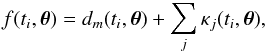 (2)where κj, with j ≥ 0, are Keplerian curves representing the reflex motion produced by an orbiting companion to the host star or the magnetic activity effect, usually appearing at the rotational frequency of the star and its harmonics (Boisse et al. 2011b). The Keplerian curves were parametrised using the orbital period (P) and eccentricity (e), velocity amplitude (K), argument of periastron, (ω) and mean longitude at a given epoch (L0). The term dm(ti,θ) is a mth-degree polynomial representing secular accelerations, which are known as stellar drifts. In principle, the physical model could contain an additional term representing the long-term stellar activity effect (i.e. the effect of stellar cycles) as done by Díaz et al. (2016). As no cycle was detected for any of our stars, this term is not included in the current model description.
Following the procedure described in Díaz et al. (2016),  was allowed to increase linearly with activity level, measured by the Hα index for SOPHIE data. The value of the additional noise for measurement i,
  takes the form
 (3)where σJ|min is the additional noise at activity minimum, which includes the systematic instrumental noise, and αJ is the sensitivity of the noise to activity level. This model has two additional parameters: σJ | min and αJ. In contrast, as ELODIE velocities are more concentrated in time, a constant jitter term was used.
The parameter priors are presented in Table A.1. The prior distributions chosen for the zero-point offset between ELODIE and SOPHIE come from the calibration presented by Boisse et al. (2012) using the B − V value listed in Table 2. Between SOPHIE and SOPHIE+, we chose a zero-centred normal distribution with a standard deviation of 10 m s-1. This comes from preliminary work done on the SOPHIE data, which indicates that once corrected for the seeing effect, the zero-point offset introduced by the upgrade is insignificant.
5.2. Posterior sampling
We sampled the posterior distributions of the model parameter using the Markov chain Monte Carlo (MCMC) described in Díaz et al. (2014). We obtained the starting point of the MCMC algorithm using a genetic algorithm included in the yorbit package (Ségransan et al. 2011; Bouchy et al. 2016). Ten independent samplers were run for each system for 500 000 iterations and these results were combined as described in Díaz et al. (2014). In this way, we obtained over 20 000 independent posterior samples for each target.
5.3. Astrometric analysis
We analysed the available Hipparcos astrometry (ESA 1997) of the four targets stars. The new Hipparcos reduction (van Leeuwen 2007) was employed to search for signatures of orbital motion in the Intermediate Astrometric Data (IAD). The analysis was performed following Sahlmann et al. (2011), where a detailed description of the method can be found.
Using the parameters of the radial velocity orbit (Table 4), the IAD was fitted with a seven-parameter model, where the free parameters are the inclination i, the longitude of the ascending node Ω, the parallax, and offsets to the coordinates and proper motions. A two-dimensional grid in i and Ω was searched for its global χ2-minimum. The statistical significance of the derived astrometric orbit is determined with a permutation test employing 1000 pseudo-orbits.
We did not detect significant orbital signal in the Hipparcos astrometry for any of the four planets. Because none of the orbital periods of the planets is fully covered by Hipparcos measurements, we are unable to set upper limits to the companion masses as we did in the past (e.g. Díaz et al. 2012). The only exception is HD 221585b, for which Hipparcos observed 94% of the orbit and where the non-detection of an astrometric signature excludes a stellar mass for the companion.
6. Results
In this section we discuss the results of the modelling of the RV data. The RV measurements are plotted together with the fitted models in Fig. 1. A summary description of the posterior distribution is given in Table 4, where the posterior mean and the equal-tailed 68.3% confidence interval is given. We also reported the 95% highest density interval (HDI) limit when the lower limit of the 95% HDI was at the limit imposed by the priors listed in Table A.1.
6.1. New companions
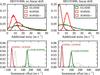 |
Fig. 4 Posterior distributions of the additional noise terms (upper panels) and instrument offsets (lower panels) for HD 191806 under two competing models: with (right column) and without (left column) a secular acceleration term (order m in Eq. (2)). In the upper panels, we depict the posterior distribution of additional noise at activity minimum for SOPHIE and SOPHIE+ (see Sect. 5.1) and the amplitude of the (constant) additional noise for ELODIE. In the lower panels, the dotted curves correspond to prior distributions. |
6.1.1. HD 191806
The model used to fit the HD 191806 RV data consisted of a single Keplerian curve plus a linear trend (i.e. j = 1 and m = 1 in Eq. (2)). The presence of a long-term trend is not obvious in the original data set and depends on the values taken by the instrument offsets. However, the model without a secular acceleration (m = 0) results in a worse fit to the data because its posterior distribution for the SOPHIE/SOPHIE+ offset peaks near –50 m s-1, i.e. far from the prior centre (see Fig. 4, left column). In other words, the model without acceleration requires an unrealistically high value of this parameter to fit the data reasonably well. As a consequence, the Bayes factor, which is computed using the techniques of Perrakis et al. (2014) and Chib & Jeliazkov (2001) (see also Díaz et al. 2016), shows that the model with the acceleration term is 280 ± 75 times more probable than the simpler model despite the use of additional parameters. Incidentally, under the model without linear drift, the amplitude of the additional noise at activity minimum, σJ | min, for SOPHIE+ has a posterior distribution similar to that of SOPHIE (Fig. 4). This would only be expected if the activity jitter dominates completely over the instrumental noise, which is not expected for this star. However, this excessive jitter term for SOPHIE+ is not punished in the Bayes factor computation because we chose flat priors for this parameter. When the m = 1 model is used, the posterior distributions of the jitter term and the offsets are as expected (Fig. 4, right column). We conclude that the velocity of HD 191806 exhibits a secular acceleration.
Under the model with a linear trend, the velocity modulation has an amplitude of 140 m s-1 and a period of 1606.3 ± 7.2 days (4.4 years). The frequency spectrum of the Hα time series of HD 191806 exhibits a peak with the same period as the RV modulation. However, as discussed in Sect. 3.1, this periodicity is not significant. The data favour a model without activity variation at this period. Furthermore, no significant variation of the bisector span was detected. It seems unlikely that stellar activity is able to produce a 140 m s-1 RV modulation without producing a variation in the line bisectors. We therefore conclude that the RV variation is due to a companion in orbit around HD 191806. Nevertheless, we remain cautious concerning the accuracy of our parameter determination, which can potentially be affected by activity. Long-term follow-up of this target should permit us to better understand the Hα variability and its effect on the system parameters.
Additionally, we detect a significant eccentricity of e = 0.259 ± 0.017. The companion around HD 191806 has therefore a minimum mass of 8.52 ± 0.63MJup. The linear trend has an amplitude of 11.4 ± 1.7 m s-1 yr-1.
6.1.2. HD 214823
The RV data of HD 214823 are adequately reproduced by a model with j = 1 and m = 0, i.e. a model with a single Keplerian curve, with an amplitude of around 280 m s-1and a period of 1877 days (5.1 years). The orbit is fully covered by the SOPHIE and SOPHIE+ data, but the ELODIE measurements help constrain the period. The velocity offset between ELODIE and SOPHIE (24 ± 19 m s-1) is in agreement with the value expected from the calibration of Boisse et al. (2012), which is 57 ± 23 m s-1(see Table A.1), but the precision is improved. In contrast, the offset between SOPHIE and SOPHIE+ is compatible with zero, as expected.
The activity level of HD 214823 seems to be decreasing (Fig. 3). Although some power is seen in the frequency spectrum of the Hα index at the period of the Keplerian curve, this is most probably due to long-term activity evolution. The highest peak in the Hα periodogram (13.1 days) agrees with the expected rotational period of the star based on the calibration by Mamajek & Hillenbrand (2008). Additionally, there are no significant signals in the bisector velocity span (Table 3). We conclude therefore that the detected radial velocity variation originates from a companion with a minimum mass mcsini = 19.4 ± 1.4MJup. HD 214823 b is therefore a brown dwarf candidate on a mildly eccentric orbit, e = 0.154 ± 0.014.
6.1.3. HD 221585
HD 221585 exhibits RV variations with an amplitude of around 28 m s-1 and a period of 1173 days (3.2 years) under the model with no secular acceleration and a single Keplerian curve. The final orbital fit of HD 221585 was only possible after the addition of the last few SOPHIE+ measurements. The reason for this is the relatively small number of SOPHIE measurements, which impeded a correct determination of the velocity offset between instruments and allowed for the presence of secular accelerations in a preliminary analysis. Here again, the posterior velocity difference between SOPHIE and SOPHIE+ is compatible with no offset, and the SOPHIE/ELODIE offset agrees with the expected value and is determined with improved precision (see discussion below).
The activity level of HD 221585 has remained unchanged for over ten years, as seen in the time series of the Hα measurements. However, we interpret the peak at 35-day period in the periodogram of the activity indexes as an indication of the stellar rotational period, which is in agreement with the expectation from the activity level measured in the Ca II H and K lines. No power is seen at periods close to that of the Keplerian curve and, furthermore, the bisector velocity span does not show any significant variability. These facts lead us to conclude that the RV variability is produced by an orbiting companion with minimum mass of mcsini = 1.61 ± 0.14MJup.
The amplitude of the reflex motion of HD 221585 is the smallest among the stars studied here. The eccentricity is therefore determined less precisely and did not lead to a significant detection. The eccentricity 95% upper limit is 0.24. The companion is at a distance of 2.3 au from its star, and is therefore unlikely that the circularisation of the orbit has occurred through tidal interaction.
6.2. Orbit update
6.2.1. HD 16175
A companion to HD 16175 was discovered by Peek et al. (2009) based on RV measurements obtained at Lick Observatory. They reported a companion on an eccentric (e = 0.59 ± 0.11), 990-day orbit with a minimum mass of 4.40 MJup. The host star is an evolved, metal-rich G0 subgiant.
We combined the Lick data with the ELODIE and SOPHIE+ data to improve the orbital and physical parameters of the system. We used a constant additional noise term for the Lick data. As we do not have any information on the velocity offset between the Lick and ELODIE or SOPHIE measurements, we used a flat prior spanning 400 m s-1 (see Table A.1). Fortunately, one Lick measurement overlaps in time with the ELODIE measurements (Fig. 1) and, therefore, the offset is constrained by the data with a precision of 2.7 m s-1.
Our results are in agreement with those of Peek et al. (2009), but the precision is improved by a factor ranging between 2 and 7 for the orbital parameters. We found a period P = 995.4 ± 2.8 days, and eccentricity e = 0.637 ± 0.020, which is slightly higher than the value reported previously, and a velocity amplitude, K = 103.5 ± 5.0 m s-1. Since no variation in the activity index nor in the bisector is seen, we conclude that this variation is due to a companion with a minimum mass of mcsini = 4.77 ± 0.37MJup.
7. Giant planets in the habitable zone
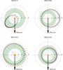 |
Fig. 5 Schematic view of the systems. The orbital plane is represented. The maximum a posteriori companion orbits are indicated with the empty black points that are equally spaced in time over the orbit. The orbital movement is counter-clockwise and angles are measured counter-clockwise from the negative x-axis. The semi-major axis of the orbit is shown as a thin grey line. The host star is at the centre and the area of the orange circle is proportional to its luminosity. The concentric circles are labelled in astronomical units and the black thick arrow points towards the observer. The filled green area is the habitable zone comprised between the “runaway greenhouse” limit and the “maximum greenhouse” limit, according to the model of Kopparapu et al. (2013b). The red area corresponds to the increased habitable zone if the outer edge is defined by the “early Mars” limit. |
Habitable zone location and average incident flux.
The stellar effective temperatures and luminosities computed as described in Sect. 3 can be used to estimate the location of the habitable zone (HZ) around each star. This is done using Eqs. (2) and (3) of Kopparapu et al. (2013b) and the erratum Kopparapu et al. (2013a) for different habitable zone limits. They are listed in Table 5. Following Kopparapu et al. (2013b) the inner edge of the HZ is taken as the distance where runaway greenhouse effect takes place. Although this is more liberal than choosing the “moist greenhouse” limit for stars hotter than around 5500 K (see their Fig. 8), the candidates presented here are closer to the outer edge of the habitable zone. For the outer edge, we chose the “maximum greenhouse” limit, where the heating effect of the greenhouse is outweighed by the Rayleigh scattering by CO2. The more liberal “early Mars” expands the outer edge only slightly (see Fig. 5).
A schematic view of the results is provided in Fig. 5. On account of their orbital eccentricity, the majority of the detected companions make excursions outside of the HZ throughout their orbit. The exception is HD 221585 b, whose entire orbit is spent within the HZ. In contrast, HD 214823 b, spends around 23% of its orbit outside the HZ. The situation is more critical for HD 191806 b, which spends 68% of its orbit outside the HZ. The situation of HD 16175 b is even more extreme with 21% of its orbit spent within the inner edge of the HZ and more than 38% spent outside the outer edge. However, Williams & Pollard (2002) argued that long-term climate stability is dictated by the mean incident flux throughout the orbit and not the length of time spent in the HZ. The mean incident flux over an orbit with respect to the mean flux received by a planet at 1 au orbiting the Sun (ℱ⊕) is 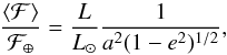 (4)where L is the stellar luminosity and a is the semi-major axis of the orbit (in au). The average incident flux is listed in Table 5.
In Fig. 6 (inspired by Fig. 8 of Kopparapu et al. 2013b) we place the resulting average incident fluxes with respect to the limiting HZ fluxes for stars with different effective temperatures Teff. The filled region is the HZ enclosed by the “moist greenhouse” limit and the “maximum greenhouse” limit, which correspond to the same region indicated in the orbit plots (Fig. 5). The solid black curve is the locus of the runaway greenhouse limit. We see that all candidates but HD 191806 b lie well within the HZ of their star. Even HD 16175 b, with its very eccentric orbit, receives an average flux that would allow liquid water to exist in the surface of a hypothetical rocky moon provided that the satellite is capable of maintaining a relatively constant temperature throughout the orbit, despite the change in insolation of a factor [(1 + e) / (1 − e)] 2 ~ 20. Hypothetical rocky satellites orbiting HD 221585 b and HD 214823 b have good prospects for habitability.
However, as mentioned above, all the target stars evolved at least slightly from their primitive position in the main sequence. Therefore, the positions of their companions in Fig. 6 are not representative of the positions during the main-sequence lifetime. Using the PARSEC tracks, we estimated the effective temperatures and effective incident fluxes when the stars were 1 Gyr of age. For this, we used the values of the stellar masses and metallicities listed in Table 2 and assumed that the companion orbits have not evolved. The past positions obtained under this hypothesis are indicated with plus signs in the diagram of Fig. 6 and connected to the current positions by straight lines. Because the stars were less luminous in the past and we assumed unchanged orbits, the companions move to the right in the diagram as we move to the past. HD 214823 b and HD 221585 b were located outside the HZ when the stars were 1 Gyr old; in contrast, the companion around HD 16175 is in the “continuously habitable” zone. This computation is, however, extremely dependent on the current stellar parameters (ages and masses) and on the stellar models used to trace the position of the stars into the past. The evolution shown in Fig. 6 does not correspond to the evolution one would guess by following the closest evolution track shown in Fig. 2 across the isochrones. This is mainly due to the discrepancy in the mass determination mentioned above. This underlines the need for accurate stellar masses and ages and the importance of the space mission PLATO (Rauer et al. 2014).
8. Summary and discussion
We detected three new companions to solar-type stars on long-period orbits and an updated orbit for the Jupiter-mass candidate HD 16175 b, which was first reported by Peek et al. (2009). The position of the companions in the mass-period diagram is not atypical (Fig. 7). HD 214823 b, with a minimum mass of 19 MJup , is a brown dwarf candidate that bears resemblance to HD 168443 c (Marcy et al. 2001) and HD 131664 b (Moutou et al. 2009). The host stars are slightly more massive than the Sun and seem to have started evolving away from the main sequence. The most evolved star studied here is HD 221585. An interpolation using the PARSEC tracks (Bressan et al. 2012; da Silva et al. 2006) gives an age of 6.6 Gyr and a radius of 1.7 R⊙. All four stars are metal rich with metallicities, [Fe/H], ranging between +0.17 and +0.30.
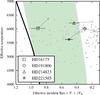 |
Fig. 6 Locus of the habitable zone in the effective temperature – incident flux plane. The green filled area is delimited on the right by the maximum greenhouse limit and on the left by the moist greenhouse limit. The solid black curve represents the position of the runaway greenhouse limit. The position of the candidate planets are marked with different symbols, as indicated in the legend. The straight lines connect the current positions of the candidates with the positions they had when their host stars were 1 Gyr old (indicated by plus signs), according to the PARSEC evolution tracks (see text for detail). The grey points are giant planets (Msini> 0.1MJup) orbiting non-evolved stars (ΔMV< 2.0; Wright 2005). |
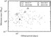 |
Fig. 7 Position of the new companions in the mass-period diagram. The grey points are giant planets (Msini> 0.1MJup) reported in the literature (Han et al. 2014) with orbital period P> 500 days orbiting non-evolved stars (ΔMV< 2.0; Wright 2005). Note that the error bars for our detections are smaller than the symbols. |
We combined data from the ELODIE, SOPHIE, and SOPHIE+ spectrographs along with observations from the Lick planet search. We took a Bayesian approach to model the radial velocity variations to include a priori knowledge on the instrument velocity offsets, whenever it was available. The case of HD 191806 illustrates the importance of including this information in the analysis. Indeed, had the SOPHIE / SOPHIE+ offset been left free, the model without an acceleration term would have resulted in a good fit, albeit with an unrealistically high value for this parameter.
To account for the noise induced by stellar activity and instrument systematics, the model included an additional white noise term. For SOPHIE data, the amplitude of the additional noise term was allowed to vary linearly with activity level. For SOPHIE+, the 95% HDI of the noise amplitude at activity minimum includes zero, which means that no additional noise is actually measured. This is probably because of the relatively low precision of the SP2 measurements (see Sect. 2); the scatter of the SOPHIE+ measurements is dominated by photon noise. HD 221585 is the least active star in our sample (⟨log R⟩ = − 4. 86) and exhibits the lowest base-level jitter for SOPHIE+: only 2.1 ± 1.4 m s-1 (upper limit 4.5 m s-1). On the contrary, for SOPHIE data taken before the upgrade, noise level in excess of the photon noise was detected. The only exception is HD 221585, which was observed only five times before the upgrade. Additionally, for all stars except for HD 16175, the most active of the sample, the slope of the error model is compatible with zero at the 95% level. This means that the additional noise term is compatible with a constant jitter. The precision improvement between SOPHIE and SOPHIE+, which is evident from the residual plots in Fig. 1, can be quantified using the posterior distributions of the additional noise term: the mean value is lower by a factor of around 3.6. As expected, the dispersion of the residuals is positively correlated with the mean activity level of the stars, ⟨log R⟩.
One attractive feature of the Bayesian analysis performed here is that it teaches us about the instruments in use. For example, the offset between ELODIE and SOPHIE was calibrated by Boisse et al. (2012) based on a sample of around 200 stars. They obtained a relationship between the offset and colour index B − V of the stars, which we used as prior information for our analysis. The posterior distributions of the SOPHIE/ELODIE offsets are in all cases narrower than the prior distribution, i.e. the current data constrain the offset better than the simple calibration. For example, in the case of HD 221585, the dispersion of the posterior distribution is only 5.5 m s-1compared to the 23 m s-1 used for the prior (Table A.1; see also Boisse et al. 2012). This is expected because the Boisse et al. (2012) calibration exhibits a dispersion in excess of the typical error of the individual measurements used to derive it. Performing the type of analysis we presented here on a large number of stars could serve as the basis for an improved calibration (for example, allowing for a dependence on stellar metallicity). Similarly, we see that when the SOPHIE data are corrected as described in Sect. 2 the velocity difference between SOPHIE and SOPHIE+ is compatible with zero. This is in agreement with the chosen prior information. However, there is a hint of a dependence on colour index B − V; the offset posterior distribution for HD 221585, the reddest star in our sample, peaks at higher values than for HD 191806 and HD 214823. To verify this dependence an analysis on a larger number of stars is warranted.
Three of the companions studied are currently in the habitable zone of their host star, which would make hypothetical rocky satellites orbiting around them a suitable place for life to develop. The best technique to find satellites of giant planets is probably the transit method (e.g. Kipping et al. 2012), however, the times of inferior conjunction of these companions are only known to a precision of between 9 and 30 days (see Table 4). Therefore, a ground-based search is likely unfeasible. On the other hand, these stars will certainly become prime targets for the follow-up space mission CHEOPS (Broeg et al. 2013) that will search for transits of these giant planets and of potentially habitable exomoons (Simon et al. 2015). An issue arises concerning the time the candidate has spent in the habitable zone during its lifetime. Indeed, all the stars studied here are slightly evolved, which means that the environment at the candidate orbital distance has changed in the recent past. Out of the four candidates reported here, only HD 16175 b would be, according to estimates based on the PARSEC stellar evolution model and the measurement of the stellar masses and metallicities in the so-called “continuously habitable” zone. The remaining candidates were not inside the habitable zone during their early main-sequence lifetimes. However, this conclusion is strongly dependent on the current age of the system, which is presently very uncertain. This stresses the importance of the space mission PLATO (Rauer et al. 2014) and the accurate determination of the masses and ages of exoplanet hosts.
These tables contain the raw measurements. The offset between the instrument zero-points was not included (see Sect. 5.1).
This is narrower than the 1.5-Å window used by Cincunegui et al. (2007b) to compute the Hα index in medium resolution spectra and also than the 1.6-Å window employed by Gomes da Silva et al. (2014). We believe that such large windows are at the base of the variability in correlation between the Hα index and Ca II H & K index reported by these authors. A thorough analysis is needed.
Precisely, the 95% HDI of the amplitude distribution contains zero.
Acknowledgments
We thank all the staff of Haute-Provence Observatory for their support at the 1.93-m telescope and on SOPHIE. This work has been carried out within the frame of the National Centre for Competence in Research “PlanetS” supported by the Swiss National Science Foundation (SNSF). J.R. acknowledges support from the CONICYT/Becas Chile 72140583. A.S. and N.C.S. acknowledge the support from Fundação para a Ciência e a Tecnologia (FCT, Portugal) in the form of grants reference UID/FIS/04434/2013 (POCI-01-0145-FEDER-007672) and PTDC/FIS-AST/1526/2014. N.C.S. was also supported by FCT through the Investigador FCT contract reference IF/00169/2012 and POPH/FSE (EC) by FEDER funding through the programme “Programa Operacional de Factores de Competitividade – COMPETE. AS is supported by the European Union under a Marie Curie Intra-European Fellowship for Career Development with reference FP7-PEOPLE-2013-IEF, number 627202. P.A.W. acknowledges the support of the French Agence Nationale de la Recherche (ANR), under programme ANR-12-BS05-0012 “Exo-Atmos”. This research has made use of the SIMBAD database and of the VizieR catalogue access tool operated at CDS, France. This research has made use of the Exoplanet Orbit Database and the Exoplanet Data Explorer at exoplanets.org.
References
- Baliunas, S. L., Donahue, R. A., Soon, W. H., et al. 1995, ApJ, 438, 269 [NASA ADS] [CrossRef] [Google Scholar]
- Baranne, A., Queloz, D., Mayor, M., et al. 1996, A&AS, 119, 373 [NASA ADS] [CrossRef] [EDP Sciences] [Google Scholar]
- Boisse, I., Eggenberger, A., Santos, N. C., et al. 2010, A&A, 523, A88 [NASA ADS] [CrossRef] [EDP Sciences] [Google Scholar]
- Boisse, I., Bouchy, F., Chazelas, B., et al. 2011a, Research, Science and Technology of Brown Dwarfs and Exoplanets: Proceedings of an International Conference held in Shangai on Occasion of a Total Eclipse of the Sun, Shangai, China, eds. E. L. Martin, J. Ge, & W. Lin, EPJ Web Conf., 16, 02003 [Google Scholar]
- Boisse, I., Bouchy, F., Hébrard, G., et al. 2011b, A&A, 528, A4 [NASA ADS] [CrossRef] [EDP Sciences] [Google Scholar]
- Boisse, I., Pepe, F., Perrier, C., et al. 2012, A&A, 545, A55 [NASA ADS] [CrossRef] [EDP Sciences] [Google Scholar]
- Bouchy, F., Hébrard, G., Udry, S., et al. 2009a, A&A, 505, 853 [NASA ADS] [CrossRef] [EDP Sciences] [Google Scholar]
- Bouchy, F., Isambert, J., Lovis, C., et al. 2009b, in EAS Publ. Ser. 37, ed. P. Kern, 247 [Google Scholar]
- Bouchy, F., Díaz, R. F., Hébrard, G., et al. 2013, A&A, 549, A49 [NASA ADS] [CrossRef] [EDP Sciences] [Google Scholar]
- Bouchy, F., Ségransan, D., Díaz, R. F., et al. 2016, A&A, 585, A46 [NASA ADS] [CrossRef] [EDP Sciences] [Google Scholar]
- Bressan, A., Marigo, P., Girardi, L., et al. 2012, MNRAS, 427, 127 [NASA ADS] [CrossRef] [Google Scholar]
- Broeg, C., Fortier, A., Ehrenreich, D., et al. 2013, in Eur. Phys. J. Web Conf., 47, 03005 [Google Scholar]
- Chib, S. & Jeliazkov, I. 2001, J. Am. Stat. Assoc., 96, 270 [CrossRef] [Google Scholar]
- Cincunegui, C., Díaz, R. F., & Mauas, P. J. D. 2007a, A&A, 461, 1107 [NASA ADS] [CrossRef] [EDP Sciences] [Google Scholar]
- Cincunegui, C., Díaz, R. F., & Mauas, P. J. D. 2007b, A&A, 469, 309 [NASA ADS] [CrossRef] [EDP Sciences] [Google Scholar]
- Courcol, B., Bouchy, F., Pepe, F., et al. 2015, A&A, 581, A38 [NASA ADS] [CrossRef] [EDP Sciences] [Google Scholar]
- Cox, A. N. 2000, Allen’s astrophysical quantities, Allen’s astrophysical quantities, 4th edn (New York: AIP Press; Springer), ed. A. N. Cox [Google Scholar]
- da Silva, L., Girardi, L., Pasquini, L., et al. 2006, A&A, 458, 609 [NASA ADS] [CrossRef] [EDP Sciences] [Google Scholar]
- Díaz, R. F., Santerne, A., Sahlmann, J., et al. 2012, A&A, 538, A113 [NASA ADS] [CrossRef] [EDP Sciences] [Google Scholar]
- Díaz, R. F., Almenara, J. M., Santerne, A., et al. 2014, MNRAS, 441, 983 [NASA ADS] [CrossRef] [Google Scholar]
- Díaz, R. F., Ségransan, D., Udry, S., et al. 2016, A&A, 585, A134 [NASA ADS] [CrossRef] [EDP Sciences] [Google Scholar]
- Dravins, D. 1982, ARA&A, 20, 61 [NASA ADS] [CrossRef] [Google Scholar]
- Dumusque, X., Lovis, C., Ségransan, D., et al. 2011, A&A, 535, A55 [NASA ADS] [CrossRef] [EDP Sciences] [Google Scholar]
- Endl, M., Hatzes, A. P., Cochran, W. D., et al. 2004, ApJ, 611, 1121 [NASA ADS] [CrossRef] [Google Scholar]
- ESA 1997, The HIPPARCOS and Tycho catalogues. Astrometric and photometric star catalogues derived from the ESA HIPPARCOS Space Astrometry Mission, 1200 [Google Scholar]
- van Leeuwen, F. 2007, HIPPARCOS, the New Reduction of the Raw Data, Astrophys. Space Sci. Lib., 350 [Google Scholar]
- Gomes da Silva, J., Santos, N. C., Boisse, I., Dumusque, X., & Lovis, C. 2014, A&A, 566, A66 [NASA ADS] [CrossRef] [EDP Sciences] [Google Scholar]
- Gregory, P. C. 2011, MNRAS, 415, 2523 [NASA ADS] [CrossRef] [Google Scholar]
- Han, E., Wang, S. X., Wright, J. T., et al. 2014, PASP, 126, 827 [NASA ADS] [CrossRef] [Google Scholar]
- Hatzes, A. P., Cochran, W. D., McArthur, B., et al. 2000, ApJ, 544, L145 [NASA ADS] [CrossRef] [Google Scholar]
- Hébrard, G., Bonfils, X., Ségransan, D., et al. 2010, A&A, 513, A69 [NASA ADS] [CrossRef] [EDP Sciences] [Google Scholar]
- Hébrard, G., Arnold, L., Forveille, T., et al. 2016, A&A, 588, A145 [NASA ADS] [CrossRef] [EDP Sciences] [Google Scholar]
- Heller, R., & Pudritz, R. 2015, A&A, 578, A19 [NASA ADS] [CrossRef] [EDP Sciences] [Google Scholar]
- Heller, R., Williams, D., Kipping, D., et al. 2014, Astrobiol., 14, 798 [NASA ADS] [CrossRef] [Google Scholar]
- Høg, E., Fabricius, C., Makarov, V. V., et al. 2000, A&A, 355, L27 [NASA ADS] [Google Scholar]
- Horner, J., & Jones, B. W. 2008, Int. J. Astrobiol., 7, 251 [NASA ADS] [CrossRef] [Google Scholar]
- Horner, J., & Jones, B. W. 2010, Astron. Geophys., 51, 16 [CrossRef] [Google Scholar]
- Jofré, E., Petrucci, R., Saffe, C., et al. 2015, A&A, 574, A50 [NASA ADS] [CrossRef] [EDP Sciences] [Google Scholar]
- Kass, R. E. & Raftery, A. E. 1995, J. Amer. Stat. Assoc., 90, 773 [Google Scholar]
- Kasting, J. F., Whitmire, D. P., & Reynolds, R. T. 1993, Icarus, 101, 108 [NASA ADS] [CrossRef] [PubMed] [Google Scholar]
- Kipping, D. M., Bakos, G. Á., Buchhave, L., Nesvorný, D., & Schmitt, A. 2012, ApJ, 750, 115 [NASA ADS] [CrossRef] [Google Scholar]
- Kopparapu, R. K., Ramirez, R., Kasting, J. F., et al. 2013a, ApJ, 770, 82 [NASA ADS] [CrossRef] [Google Scholar]
- Kopparapu, R. K., Ramirez, R., Kasting, J. F., et al. 2013b, ApJ, 765, 131 [NASA ADS] [CrossRef] [Google Scholar]
- Laakso, T., Rantala, J., & Kaasalainen, M. 2006, A&A, 456, 373 [NASA ADS] [CrossRef] [EDP Sciences] [Google Scholar]
- Lindegren, L., & Dravins, D. 2003, A&A, 401, 1185 [NASA ADS] [CrossRef] [EDP Sciences] [Google Scholar]
- LoCurto, G., Pepe, F., Avila, G., et al. 2015, The Messenger, 162, 9 [NASA ADS] [Google Scholar]
- Lovis, C., Dumusque, X., Santos, N. C., et al. 2011a, A&A, submitted [arXiv:1107.5325] [Google Scholar]
- Lovis, C., Ségransan, D., Mayor, M., et al. 2011b, A&A, 528, A112 [NASA ADS] [CrossRef] [EDP Sciences] [Google Scholar]
- Mamajek, E. E., & Hillenbrand, L. A. 2008, ApJ, 687, 1264 [NASA ADS] [CrossRef] [Google Scholar]
- Marcy, G. W., Butler, R. P., Vogt, S. S., et al. 2001, ApJ, 555, 418 [NASA ADS] [CrossRef] [Google Scholar]
- Mauas, P. J. D., & Falchi, A. 1994, A&A, 281, 129 [NASA ADS] [Google Scholar]
- Mayor, M., Pepe, F., Queloz, D., et al. 2003, The Messenger, 114, 20 [NASA ADS] [Google Scholar]
- Meunier, N., & Lagrange, A.-M. 2013, A&A, 551, A101 [NASA ADS] [CrossRef] [EDP Sciences] [Google Scholar]
- Meunier, N., Desort, M., & Lagrange, A.-M. 2010, A&A, 512, A39 [NASA ADS] [CrossRef] [EDP Sciences] [Google Scholar]
- Montes, D., Fernandez-Figueroa, M. J., de Castro, E., & Cornide, M. 1995, A&A, 294, 165 [NASA ADS] [Google Scholar]
- Moutou, C., Mayor, M., Lo Curto, G., et al. 2009, A&A, 496, 513 [NASA ADS] [CrossRef] [EDP Sciences] [Google Scholar]
- Moutou, C., Hébrard, G., Bouchy, F., et al. 2014, A&A, 563, A22 [NASA ADS] [CrossRef] [EDP Sciences] [Google Scholar]
- Neveu-VanMalle, M., Queloz, D., Anderson, D. R., et al. 2016, A&A, 586, A93 [NASA ADS] [CrossRef] [EDP Sciences] [Google Scholar]
- Noyes, R. W., Hartmann, L. W., Baliunas, S. L., Duncan, D. K., & Vaughan, A. H. 1984, ApJ, 279, 763 [NASA ADS] [CrossRef] [Google Scholar]
- Pasquini, L., & Pallavicini, R. 1991, A&A, 251, 199 [NASA ADS] [Google Scholar]
- Peek, K. M. G., Johnson, J. A., Fischer, D. A., et al. 2009, PASP, 121, 613 [NASA ADS] [CrossRef] [Google Scholar]
- Pepe, F., Mayor, M., Galland, F., et al. 2002, A&A, 388, 632 [NASA ADS] [CrossRef] [EDP Sciences] [Google Scholar]
- Perrakis, K., Ntzoufras, I., & Tsionas, E. G. 2014, Computational Statistics & Data Analysis, 77, 54 [Google Scholar]
- Perruchot, S., Kohler, D., Bouchy, F., et al. 2008, in SPIE Conf. Ser. 7014 [Google Scholar]
- Perruchot, S., Bouchy, F., Chazelas, B., et al. 2011, in Techniques and Instrumentation for Detection of Exoplanets V, SPIE, 8151, 815115 [Google Scholar]
- Porter, S. B., & Grundy, W. M. 2011, ApJ, 736, L14 [NASA ADS] [CrossRef] [Google Scholar]
- Queloz, D., Mayor, M., Weber, L., et al. 2000, A&A, 354, 99 [NASA ADS] [Google Scholar]
- Queloz, D., Henry, G. W., Sivan, J. P., et al. 2001, A&A, 379, 279 [NASA ADS] [CrossRef] [EDP Sciences] [Google Scholar]
- Rauer, H., Catala, C., Aerts, C., et al. 2014, Exp. Astron., 38, 249 [NASA ADS] [CrossRef] [Google Scholar]
- Robertson, P., Endl, M., Cochran, W. D., & Dodson-Robinson, S. E. 2013, ApJ, 764, 3 [NASA ADS] [CrossRef] [Google Scholar]
- Robertson, P., Mahadevan, S., Endl, M., & Roy, A. 2014, Science, 345, 440 [NASA ADS] [CrossRef] [Google Scholar]
- Rowe, J. F., Bryson, S. T., Marcy, G. W., et al. 2014, ApJ, 784, 45 [NASA ADS] [CrossRef] [Google Scholar]
- Sahlmann, J., Ségransan, D., Queloz, D., et al. 2011, A&A, 525, A95 [NASA ADS] [CrossRef] [EDP Sciences] [Google Scholar]
- Santerne, A., Díaz, R. F., Almenara, J.-M., et al. 2015, MNRAS, 451, 2337 [NASA ADS] [CrossRef] [Google Scholar]
- Santos, N. C., Mayor, M., Naef, D., et al. 2000, A&A, 361, 265 [NASA ADS] [Google Scholar]
- Santos, N. C., Mayor, M., Naef, D., et al. 2002, A&A, 392, 215 [NASA ADS] [CrossRef] [EDP Sciences] [Google Scholar]
- Santos, N. C., Israelian, G., & Mayor, M. 2004, A&A, 415, 1153 [NASA ADS] [CrossRef] [EDP Sciences] [Google Scholar]
- Santos, N. C., Gomes da Silva, J., Lovis, C., & Melo, C. 2010, A&A, 511, A54 [NASA ADS] [CrossRef] [EDP Sciences] [Google Scholar]
- Santos, N. C., Sousa, S. G., Mortier, A., et al. 2013, A&A, 556, A150 [NASA ADS] [CrossRef] [EDP Sciences] [Google Scholar]
- Ségransan, D., Udry, S., Mayor, M., et al. 2010, A&A, 511, A45 [NASA ADS] [CrossRef] [EDP Sciences] [Google Scholar]
- Ségransan, D., Mayor, M., Udry, S., et al. 2011, A&A, 535, A54 [NASA ADS] [CrossRef] [EDP Sciences] [Google Scholar]
- Sellke, T., Bayarri, M., & Berger, J. O. 2001, The American Statistician, 55, 62 [CrossRef] [Google Scholar]
- Simon, A. E., Szabó, G. M., Kiss, L. L., Fortier, A., & Benz, W. 2015, PASP, 127, 1084 [NASA ADS] [CrossRef] [Google Scholar]
- Sousa, S. G., Santos, N. C., Mayor, M., et al. 2008, A&A, 487, 373 [NASA ADS] [CrossRef] [EDP Sciences] [MathSciNet] [Google Scholar]
- Sousa, S. G., Santos, N. C., Mortier, A., et al. 2015, A&A, 576, A94 [NASA ADS] [CrossRef] [EDP Sciences] [Google Scholar]
- Torres, G. 2010, AJ, 140, 1158 [NASA ADS] [CrossRef] [Google Scholar]
- Torres, G., Andersen, J., & Giménez, A. 2010, A&ARv, 18, 67 [Google Scholar]
- Vogt, S. S., Allen, S. L., Bigelow, B. C., et al. 1994, in Instrumentation in Astronomy VIII, eds. D. L. Crawford, & E. R. Craine, SPIE Conf. Ser., 2198, 362 [Google Scholar]
- Williams, D. M., & Pollard, D. 2002, Int. J. Astrobiol., 1, 61 [NASA ADS] [CrossRef] [Google Scholar]
- Williams, D. M., Kasting, J. F., & Wade, R. A. 1997, Nature, 385, 234 [NASA ADS] [CrossRef] [PubMed] [Google Scholar]
- Wilson, P. A., Hébrard, G., Santos, N. C., et al. 2016, A&A, 588, A144 [NASA ADS] [CrossRef] [EDP Sciences] [Google Scholar]
- Wright, J. T. 2005, PASP, 117, 657 [NASA ADS] [CrossRef] [Google Scholar]
- Wright, J. T., Roy, A., Mahadevan, S., et al. 2013, ApJ, 770, 119 [NASA ADS] [CrossRef] [Google Scholar]
Appendix A: Prior distributions
Parameter prior distributions.
Appendix B: Radial velocity tables
Radial velocity measurements of HD 16175.
Radial velocity measurements of HD 191806.
Radial velocity measurements of HD 214823.
Radial velocity measurements of HD 221585.
All Tables
Basic characteristics of the ELODIE, SOPHIE, and SOPHIE+ observations of the four target stars.
Results of the bisector analysis for SOPHIE and SOPHIE+ data. χ2 statistics under the null hypothesis of no bisector variation.
All Figures
|
Fig. 1 Radial velocity data and model fits. The green points represent ELODIE data, and the red empty and filled circles represent SOPHIE and SOPHIE+ data, respectively. The empty black points are Lick Observatory data. In the upper panel of each plot, the solid thick black curve is the maximum a posteriori physical model. The blue curves are the 95% highest density interval (HDI) for the complete model, computed as described in Díaz et al. (2016) and Gregory (2011). The model posterior mean is represented by solid thin grey curve. The stellar drift or systemic velocity is shown as a thick grey line with the 95% (HDI) shown with dotted grey lines. |
| In the text | |
|
Fig. 2 Position of the four target stars in the luminosity-effective temperature plane. The PARSEC theoretical tracks (Bressan et al. 2012) are plotted using shades of grey for different initial stellar masses labelled in solar units at the bottom of each track. The corresponding isochrones are plotted as dotted lines and labelled in light grey. |
| In the text | |
|
Fig. 3 Top row: time series of the Hα activity index. The green points correspond to ELODIE observations, and red empty symbols and red filled symbols are for SOPHIE and SOPHIE+, respectively. The same scale is used for all stars to ease comparison. Bottom row: generalised Lomb-Scargle periodogram for the SOPHIE and SOPHIE+ Hα index. It was assumed that no offset exists between the index measurement of SOPHIE and SOPHIE+. The red vertical dotted lines signal the position of the highest peaks whose periods are annotated, the blue shaded areas represent the 2σ intervals for the stellar rotational periods listed in Table 2, and the green vertical dashed lines corresponds to the maximum a posteriori orbital period of the orbiting companions. |
| In the text | |
|
Fig. 4 Posterior distributions of the additional noise terms (upper panels) and instrument offsets (lower panels) for HD 191806 under two competing models: with (right column) and without (left column) a secular acceleration term (order m in Eq. (2)). In the upper panels, we depict the posterior distribution of additional noise at activity minimum for SOPHIE and SOPHIE+ (see Sect. 5.1) and the amplitude of the (constant) additional noise for ELODIE. In the lower panels, the dotted curves correspond to prior distributions. |
| In the text | |
|
Fig. 5 Schematic view of the systems. The orbital plane is represented. The maximum a posteriori companion orbits are indicated with the empty black points that are equally spaced in time over the orbit. The orbital movement is counter-clockwise and angles are measured counter-clockwise from the negative x-axis. The semi-major axis of the orbit is shown as a thin grey line. The host star is at the centre and the area of the orange circle is proportional to its luminosity. The concentric circles are labelled in astronomical units and the black thick arrow points towards the observer. The filled green area is the habitable zone comprised between the “runaway greenhouse” limit and the “maximum greenhouse” limit, according to the model of Kopparapu et al. (2013b). The red area corresponds to the increased habitable zone if the outer edge is defined by the “early Mars” limit. |
| In the text | |
|
Fig. 6 Locus of the habitable zone in the effective temperature – incident flux plane. The green filled area is delimited on the right by the maximum greenhouse limit and on the left by the moist greenhouse limit. The solid black curve represents the position of the runaway greenhouse limit. The position of the candidate planets are marked with different symbols, as indicated in the legend. The straight lines connect the current positions of the candidates with the positions they had when their host stars were 1 Gyr old (indicated by plus signs), according to the PARSEC evolution tracks (see text for detail). The grey points are giant planets (Msini> 0.1MJup) orbiting non-evolved stars (ΔMV< 2.0; Wright 2005). |
| In the text | |
|
Fig. 7 Position of the new companions in the mass-period diagram. The grey points are giant planets (Msini> 0.1MJup) reported in the literature (Han et al. 2014) with orbital period P> 500 days orbiting non-evolved stars (ΔMV< 2.0; Wright 2005). Note that the error bars for our detections are smaller than the symbols. |
| In the text | |
Current usage metrics show cumulative count of Article Views (full-text article views including HTML views, PDF and ePub downloads, according to the available data) and Abstracts Views on Vision4Press platform.
Data correspond to usage on the plateform after 2015. The current usage metrics is available 48-96 hours after online publication and is updated daily on week days.
Initial download of the metrics may take a while.