| Issue |
A&A
Volume 591, July 2016
|
|
|---|---|---|
| Article Number | A1 | |
| Number of page(s) | 16 | |
| Section | Extragalactic astronomy | |
| DOI | https://doi.org/10.1051/0004-6361/201628093 | |
| Published online | 01 June 2016 | |
Morphological classification of local luminous infrared galaxies
1 Department of Physics, University of Crete, 71003 Heraklion, Greece
e-mail: This email address is being protected from spambots. You need JavaScript enabled to view it.
2 IAASARS, National Observatory of Athens, 15236 Penteli, Greece
3 Núcleo de Astronomía de la Facultad de Ingeniería, Universidad Diego Portales, Av. Ejército Libertador 441, Santiago, Chile
4 Spitzer Science Center, Calfornia Institute of Technology, MS 220-6, Pasadena, CA 91125, USA
5 CSIRO Astronomy and Space Science, ATNF, PO Box 76, Epping 1710, Australia
6 Infrared Processing and Analysis Center, California Institute of Technology, MS 100-22, Pasadena, CA 91125, USA
7 CEA Saclay, DSM/Irfu/Service d’Astrophysique, Orme des Merisiers, 91191 Gif-sur-Yvette Cedex, France
8 Department of Physics, Virginia Tech, Blacksburg, VA 24061, USA
9 Department of Astronomy, University of Virginia, Charlottesville, VA 22904, USA
10 National Radio Astronomy Observatory, Charlottesville, VA 22903, USA
Received: 8 January 2016
Accepted: 22 February 2016
Abstract
We present analysis of the morphological classification of 89 luminous infrared galaxies (LIRGs) from the Great Observatories All-sky LIRG Survey (GOALS) sample, using non-parametric coefficients and compare their morphology as a function of wavelength. We rely on images that were obtained in the optical (B- and I-band) as well as in the infrared (H-band and 5.8 μm). Our classification is based on the calculation of Gini and the second order of light (M20) non-parametric coefficients, which we explore as a function of stellar mass (M⋆), infrared luminosity (LIR), and star formation rate (SFR). We investigate the relation between M20, the specific SFR (sSFR) and the dust temperature (Tdust) in our galaxy sample. We find that M20 is a better morphological tracer than Gini, as it allows us to distinguish systems that were formed by double systems from isolated and post-merger LIRGs. The effectiveness of M20 as a morphological tracer increases with increasing wavelength, from the B to H band. In fact, the multi-wavelength analysis allows us to identify a region in the Gini-M20 parameter space where ongoing mergers reside, regardless of the band used to calculate the coefficients. In particular, when measured in the H band, a region that can be used to identify ongoing mergers, with minimal contamination from LIRGs in other stages. We also find that, while the sSFR is positively correlated with M20 when measured in the mid-infrared, i.e. star-bursting galaxies show more compact emission, it is anti-correlated with the B-band-based M20. We interpret this as the spatial decoupling between obscured and unobscured star formation, whereby the ultraviolet/optical size of an LIRG experience an intense dust-enshrouded central starburst that is larger that in the mid-infrared since the contrast between the nuclear to the extended disk emission is smaller in the mid-infrared. This has important implications for high redshift surveys of dusty sources, where sizes of galaxies are routinely measured in the rest-frame ultraviolet.
Key words: Galaxy: structure / infrared: galaxies / galaxies: evolution / galaxies: general / galaxies: starburst
© ESO, 2016
1. Introduction
One of the remaining questions in extragalactic astronomy is how matter in the Universe assembled itself into the structures we see today. An approach to tackle this question is to study the formation and evolution of galaxies, since they are luminous beacons of the baryon content of the Universe. Galaxy morphology, which traces how the electromagnetic emission of the various physical processes is distributed across a galaxy, can be used to study how galaxies evolve and which is the dominant mechanism shaping this evolution. Fundamental properties of galaxies, such as their mass, baryonic content, star formation history, interaction state, and environment are intimately connected with galaxy morphology (Dressler 1980; Roberts & Haynes 1994; Kennicutt 1998; Strateva et al. 2001; Wuyts et al. 2011). Morphological studies can be used to constrain the theoretical models of galaxy evolution.
Traditionally the so-called Hubble Tuning Fork (Hubble 1926) provides significant information about the morphology of bright and massive galaxies in the local Universe and is closely correlated with galaxy physical properties as stellar mass (M⋆), color, star formation rate (SFR) and relative dominance of a central bulge (Roberts & Haynes 1994). However, using it to classify galaxies at z> 1 is challenging owing to limitations in angular resolution and the progressive decrease in the signal to noise (S/N) as a result of both the surface brightness dimming and the sampling of shorter wavelengths at a given observed band-pass (van den Bergh et al. 1996; Dickinson 2000). A number of optical studies observed systems at z> 2 with the Hubble Space Telescope (HST), by sampling their rest-frame ultraviolet (UV) emission, which revealed that many high-redshift galaxies exhibit irregular shapes and do not follow the typical Hubble types (Lotz et al. 2004, 2006; Papovich et al. 2005; Conselice et al. 2008). As a result, other methods using parametric coefficients, such as the Sersic index (n; Sersic et al. 1968) or non-parametric coefficients, like Gini and M20 (Abraham et al. 2003; Lotz et al. 2004) were developed to quantify the morphology of a galaxy.
At z ~ 1, corresponding to a so-called look-back time of nearly 8 Gyr, luminous infrared galaxies (LIRGs) begin to dominate the IR background and the star formation rate density (SFRD – Magnelli et al. 2013). These galaxies emit a higher fraction of energy in the infrared (IR) spectrum (~5–500 μm) than at all other wavelengths combined. A LIRG by definition emits more than 1011L⊙ in the IR (8–1000 μm) part of the electromagnetic spectrum, while, a more luminous system, emitting more than 1012L⊙, is called ultraluminous infrared galaxy (ULIRG; Sanders & Mirabel 1996). The power source of most local (U)LIRGs is a mixture of accretion onto an Active Galactic Nucleus (AGN) and a circumnuclear starburst, both of which are fueled by large quantities of high density molecular gas that has been funneled into the merger nucleus. In the process of a violent interaction of two spiral galaxies, hydrogen clouds that were initially distributed throughout the galactic disc could move to the centre, which forces the gas to become concentrated. Numerical simulations of colliding galaxies (Barnes 1992; Mihos & Hernquist 1996; Hopkins et al. 2008) show that the gas and stars react differently during a merger. The gas tends to move out in front of the stars as they orbit the galactic centre. Furthermore, gravitational torques on the gas reduce its angular momentum, causing it to plunge toward the galactic centre. As the two galaxies begin to merge, more angular momentum is lost and the concentrated circumnuclear gas feeds a massive starburst and/or an AGN.
Observations with the Infrared Space Observatory (ISO) and Spitzer Space Telescope showed that they contribute up to 50% of the cosmic infrared background, which dominates the SFR of the Universe at z ~ 1 (Elbaz et al. 2002; Le Floc’h et al. 2005; Caputi et al. 2007; Magnelli et al. 2009). Despite the rarity of (U)LIRGs in the local Universe, their study is of paramount importance as they allow an exploration of their detailed morphologies that cannot be made (owing to resolution limitations) at higher redshifts, where they are order of magnitudes more common (Blain et al. 2002; Chapman et al. 2005).
Furthermore, (U)LIRGs are strongly related with the evolution of massive galaxies. Both major and minor mergers are important in the morphological transformation of galaxies since they transform spiral disks into red and spheroids, building the high mass end of the stellar mass function, mostly at moderate to low redshifts (Williams et al. 2011). In particular, a system of two spiral galaxies that interact dynamically will pass through a violent stage, where the spiral arms and the disc of both galaxies will be destroyed and, as consequence of the violent relaxation the population of the stars, will relax to an r1/4 profile, which is a characteristic distribution of an elliptical galaxy (i.e. Hjorth & Madsen 1991; Hopkins et al. 2009). As a consequence, unlike high-z (U)LIRGs, which are mainly isolated systems with extended gas rich disks that form stars intensely, local LIRGs exhibit a large range of morphologies, from isolated galaxies to interacting pairs and mergers.
The morphological study of LIRGs across a wide wavelength range can provide information on the dynamical history of galaxies (i.e. Lotz et al. 2004; Petty et al. 2014). When combined with spectra or spectral energy distribution (SEDs), the morphologies indicate how galactic environment (or the merger history) has influenced star formation (SF). In particular, UV light originates from young massive OB stars in star-forming regions, while the optical light is mainly emitted by less massive stars. The near infrared (NIR) part of the electromagnetic spectrum unveils the location of older stellar populations that are responsible for the bulk of the total mass.
With the advent of a new generation of telescopes such as James Webb Space Telescope (JWST; Gardner 2006), Euclid (Amiaux et al. 2012), large Synoptic Survey Telescope (LSST; LSST Dark Energy Science Collaboration 2012) and the Dark Energy Survey (Frieman & Dark Energy Survey Collaboration 2013), huge amounts of data for millions of galaxies will be available at higher redshifts. It will be essential to have robust tools to make automatic morphological and structural classifications. In this paper, we investigate the connection of the local LIRG morphologies with other physical properties and pave the way for studying their high-z analogues. Our motivation is to refine the morphological method of Gini and M20 for galaxies that are dusty and that suffer an ongoing merger stage.
The paper is organised as follows. In Sect. 2 we describe the data. The morphological diagnostics are described in the Sect. 3. In Sect. 4 we present a summary of the analysis we performed to calculate the non-parametric coefficients. We present our results in Sect. 5 and discuss them in Sect. 6 when we compare our findings with other similar studies. Finally, we summarize our conclusions in Sect. 7. In Appendix A, we also provide the Gini and M20 values of our sample, using the full B- and I-band field of view (FoV), while in Appendix B, we provide a brief discussion based on the values of M50 coefficient.
2. Sample and data
2.1. Sample
The sample, upon which we base our analysis, consists of 89 LIRGs and ULIRGs from the Great Observatories All-sky LIRG Survey (GOALS; Armus et al. 2009). GOALS is a sample of 202 LIRGs selected from the IRAS Bright Galaxy Sample (RBGS; Sanders et al. 2003) and spans a redshift range of 0.009 <z< 0.088. The RBGS contains all the extragalactic objects with S60> 5.24 Jy observed by IRAS at galactic latitudes | b | ° > 5. The infrared luminosities of our 89 LIRGs lie above the value of log (LIR/L⊙) > 10.44 , the luminosity at which the local space density of LIRGs exceeds that of optically selected galaxies. These galaxies are the most luminous members of the GOALS sample and, predominantly, they are mergers and strongly interacting systems. The range of infrared luminosity is 10.44 < log (LIR/L⊙) < 12.43, with a median of 11.62. The measurements of LIR were taken from Díaz-Santos et al. (2013). Our final GOALS sample contains 89 galaxies.
2.2. Data
All galaxies in our sample have imaging obtained with the Advanced Camera for Surveys (ACS), the Wield Field Camera (WFC), the Near Infrared Camera and Multi-Object Spectrometer (NICMOS) and the Wide Field Camera 3 (WFC3) of the HST. Additionally, mid-IR (MIR) imaging is available with the Infrared Array Camera (IRAC) of Spitzer.
2.2.1. ACS HST observations
Our sample has been imaged with the ACS/WFC, using the F435W (B) and F814W (I) broad-band filters (GO program 10592, PI: A. Evans: see Evans et al. 2013). The F435W and F814W observations were performed using three- and two-point line dither patterns, respectively. The processed B- and I-band images of our sample have a large 202′′ × 202′′ FoV and was selected to capture the full extent of each interaction in one HST pointing. These filters have pixel scales of 0.05′′. At the median redshift of our sample (z = 0.033), 1′′ corresponds to ~660 pc, hence the ACS FoV covers a projected area of ~133 kpc ×133 kpc. The B band has λcen = 4297 Å and width of 1038 Å. Accordingly, the I band has λcen = 8333Å and width of 2511 Å. Further details of the observations and data reduction are described in Kim et al. (2013).
2.2.2. HST NICMOS observations
HST images with NICMOS/NIC2 were obtained using the F160W filter for 80 LIRGs. The data were collected using Camera NIC2 with a FoV of 19.3′′ × 19.5′′, a pixel size of 0.075′′ and are dithered to yield a total field area of typically 30′′ × 25′′. We note that NICMOS failed during the execution of this program, so that not all targets in the complete sample of 89 LIRGs were observed. The remaining nine were observed with WFC3, which has a wider FoV of 123′′ × 136′′ and a pixel size of 0.13′′. (See Haan et al. 2011, hereafter H11) for more details on the NICMOS data reduction.)
2.2.3. IRAC observations
IRAC is a four-channel camera (Fazio et al. 2004) on board Spitzer, that provides 5.2′ × 5.2′ images at 3.6, 4.5, 5.8, and 8 μm. In our analysis, we used the images of IRAC channel 3 at 5.8 μm. The detector has 256 × 256 pixels, with a pixel size of 1.2′′, corresponding to 844 pc for the median sample redshift.
3. Morphological diagnostics
A number of methods are used to describe the morphology of galaxies, based on the distribution of their emitted radiation. Visual morphology (Sandage 2005; Lintott et al. 2011) is the traditional approach to understanding the structure of galaxies. The major classification system in use today was proposed by Hubble (1926) and updated by de Vaucouleurs (1959) and Sandage (1961, 1975)1. On the other hand, computer algorithms have been developed to quantify the morphology of galaxies in a faster and, possibly, less biased manner (Schutter & Shamir 2015). As well as the visual and algorithmic way of characterising morphologies, galaxies can also be classified using various proxies with either parametric or non-parametric coefficients.
3.1. Methods using parametric coefficients
This type of method requires a prescribed analytic function to quantify the morphological type. This analytical function is used to model the projected light distribution and quantify the galaxy morphology with a few parameters. Historically one of the first ways to classify the structure was based on integrated light profiles. With this method, a single or multiple components can be used to model the galaxy profile (Blanton et al. 2003; Allen et al. 2006; Häußler et al. 2013). Sersic et al. (1968) empirically derived the following function to describe the radial surface brightness profile: ![Mathematical equation: \begin{equation} I(r) ~ = ~ I_{\rm e} \exp \left\{ -b_{n} \left[\left( \frac{r}{r_{\rm e}} \right)^{1/n} -1 \right] \right\} , \end{equation}](/articles/aa/full_html/2016/07/aa28093-16/aa28093-16-eq38.png) (1)where re is the effective or half-light radius, Ie is the intensity at the effective radius, n is the Sersic index, and bn is a function of n (Graham & Driver 2005). The term re relates to the physical size of the galaxy and n gives an indication of the concentration of the light distribution. The value of n is used to describe galactic structures such as bars n ~ 0.5, disks n ~ 1, bulges (1.5 <n< 10), and even the light profile of elliptical galaxies (1.5 <n< 20).
(1)where re is the effective or half-light radius, Ie is the intensity at the effective radius, n is the Sersic index, and bn is a function of n (Graham & Driver 2005). The term re relates to the physical size of the galaxy and n gives an indication of the concentration of the light distribution. The value of n is used to describe galactic structures such as bars n ~ 0.5, disks n ~ 1, bulges (1.5 <n< 10), and even the light profile of elliptical galaxies (1.5 <n< 20).
3.2. Methods using non-parametric coefficients
Non-parametric methods do not assume an analytical function for the description of the distribution of light in a galaxy. For that particular reason they can be applied to spiral or elliptical galaxies, as well as to disturbed systems that display features of dynamical interaction, such as tidal tales or bridges. Furthermore, non-parametric coefficients are less affected by limitations of resolution and can be measured out to high redshifts, making them ideal for exploring galaxy evolution across cosmic time (Conselice 2014). Since most (U)LIRGs are members of interacting systems and they often exhibit irregular shapes, our analysis is based on non-parametric coefficients.
There are many non-parametric coefficients in the literature that can be applied to morphological studies. One of them, the CAS classification system has been used extensively during the last decade. The three coefficients of CAS are the following: the concentration index (C), which was developed by Abraham et al. (1994, 1996), measures the ratio of the inner and outer part of the light in a galaxy and it correlates with the bulge to disc (B/D) galaxy ratio. Schade et al. (1995) defined the asymmetry (A) coefficient and used it to automatically distinguish spirals from ellipticals and galaxies with irregular shapes. Lotz et al. (2004) showed that galaxies with elliptical light profiles have low asymmetries, those with spiral arms are more asymmetric and finally extremely irregular and merging galaxies are typically highly asymmetric. The last coefficient, smoothness (S), was introduced by Conselice (2003). Smoothness is a good indicator of clumpiness of small-scale structures of galaxies and is related to star formation regions.
The most widespread non-parametric coefficients used is the Gini and the second-order moment-of-light distribution (M20). The Gini coefficient is based on the Lorenz curve, the rank ordered cumulative distribution function of a population’s wealth. It was proposed in 1912 by the Italian statistician and sociologist Corrado Gini who used it to measure the inequality of the levels of income in a society. Abraham et al. (2003) extended the application of Gini coefficient in the morphology of galaxies, replacing the income of the society with the pixel values of a galaxy image. For the majority of local galaxies, the Gini coefficient is correlated with C and increases with the fraction of light in a compact (central) component. Gini is defined as:  (2)where
  is the mean flux value, fi is the flux of the i-pixel and k is the number of pixels assigned to the galaxy. The values of Gini range from 0 to 1. When a galaxy has a uniform flux distribution of pixels, the Gini coefficient is close to zero. In an extreme case, when the light of the galaxy concentrates in just a few pixels, Gini is close to unity.
In addition, M20 traces the spatial distribution of any bright nuclei, bars, spiral arms, and off-centre star clusters (Lotz et al. 2004). The definition of the M20 is given by the following formula:  (3)while
 (4)The total second-order moment Mtotal is the flux in each pixel fi multiplied by the squared distance to the centre of the galaxy, summed over all pixels assigned to the galaxy:
 ![Mathematical equation: \begin{eqnarray} M_{\rm total}=\sum{M_{i}}=\sum{f_{i}\left[(x_{i}-x_{\rm c})^{2}+(y_{i}-y_{\rm c})^{2}\right]} , \end{eqnarray}](/articles/aa/full_html/2016/07/aa28093-16/aa28093-16-eq54.png) (5)where xc, yc is the galaxy’s centre and fi is the flux of pixel xi, yi. The centre is computed by finding xc, yc, such that Mtotal is minimized. A disk galaxy with bright regions in the spiral arms or a more spatially extended object corresponds to M20 values close to zero. Conversely, a galaxy with a bright bulge, single, or double nucleus (a more compact object), takes more negative M20 values.
(5)where xc, yc is the galaxy’s centre and fi is the flux of pixel xi, yi. The centre is computed by finding xc, yc, such that Mtotal is minimized. A disk galaxy with bright regions in the spiral arms or a more spatially extended object corresponds to M20 values close to zero. Conversely, a galaxy with a bright bulge, single, or double nucleus (a more compact object), takes more negative M20 values.
Since our galaxies exhibit characteristics of merging in their light distributions and many bright regions would spread around the centre of NIR light, we decided to extend our analysis by also calculating the M50 non-parametric coefficient. The limit of 50% of total flux in the definition of M50 could reveal more bright regions and possibly classify our sample in a more accurate way (see Appendix A for details).
We calculate Gini as follows: we sort the pixel values from minimum to maximum. The pixels are divided into two, equal in number, separate groups. The first 50% are the faint pixels and the remaining 50% are the brighter ones. The summation has k terms (where k is the number of the pixels inside the segmentation map). The Gini coefficient gives negative values in the faint pixels and positive to the bright ones. With this approach, Gini is calculated by summing the difference between the brightest and the faintest pixel, the second brightest and second faintest pixel, etc. The final step is to divide the difference with the term of |fi|k(k−1) in order to normalize the result and get the Gini coefficient.
The steps for the M20 calculation are as follows: we arrange the pixel values in decreasing order of flux and we calculate the term Mi for every pixel of the galaxy. We define the centre of the galaxy xc, yc as the point that represent the weighted centre of light. We calculate the numerator of the term inside the logarithm ∑ Mi, adding the moments of light of every pixel until the summed flux of the pixels reach the 20% of the total flux of the segmentation map. Finally, we calculate the M20 coefficient. As the argument of the logarithm decreases (few pixels are needed to reach the 20% of the total flux) the M20 coefficient becomes more negative and the galaxy is characterised as compact. Conversely, as the numerator does not differ greatly with the denominator, the number is bigger, the logarithm approaches values close to zero, and the galaxy has a more extended morphology. The important terms which are relevant on M20 calculation are the number of pixels required to reach the 20% of the total flux, the distance of these pixels from the centre, and the relative difference between the flux of the brightest pixel (it usually lies in the centre of the galaxy) and the flux of the fainter outer pixels of the galaxy.
4. Analysis
4.1. Constructing the segmentation map
Lotz et al. (2004) studied the Gini, M20 values of a sample of local galaxies in both NUV and optical wavelengths. Their sample included galaxies with various morphological type, i.e. spirals, ellipticals, irregulars (Irr) and also (U)LIRGs. They identify the pixels that belong to each galaxy with a technique known as the construction of the segmentation map. The general idea is to set a flux threshold in every image of the galaxy. If the pixels of the image have a value above that limit, we assume that they belong to the galaxy. The method requires a calculation of a characteristic radius of the galaxy. Most common are the definition of the Holmberg radius, the effective radius and the Petrosian radius (Petrosian 1976). The Petrosian radius is based on a curve of growth and, therefore, is less affected by the (1 + z)4 surface brightness-dimming of distant galaxies. For our analysis, we choose the Petrosian radius, which gives the opportunity to measure a characteristic radius of every galaxy, independent of its distance. The equation that gives the Petrosian radius of a galaxy is the following:  (6)where η is typically set to 0.2. The Petrosian radius (rP) is the radius at which the surface brightness at rP is 20% of the mean surface brightness inside rP. The surface brightness μ(rP) is measured for increasing circular apertures as the Petrosian radius that was determined by the curve of growth within circular apertures. We measure the flux inside an annulus and divide this with the area of the annulus. The mean surface brightness
  is the total flux inside an aperture divided by the area of the aperture.
Firstly, the image must be sky-subtracted and external sources, like field stars or other galaxies must be removed. We define circular apertures around the brightest pixel in the H-band and calculate the associated Petrosian radius. Furthermore, we convolve the cleaned galaxy image with a Gaussian of standard deviation σ = (rP/ 5), similarly to Lotz et al. (2004), to better trace low-surface brightness pixels. The pixels assigned to the galaxy must satisfy two conditions. Firstly, their flux must be greater than the μ(rP) in the smoothed image. Secondly, we define a 3 × 3 pixel area as the neighbourhood for every pixel, we measure the flux for every neighbor and, if the flux difference between the central and every neighbouring pixel is less than 10σ, then we add the pixel to the segmentation map. Finally, the map is applied to the cleaned but unsmoothed image and the pixels assigned to the galaxy are used to compute the Gini and M20 coefficients. In Fig. 1 we show the initial image and the segmentation map of NGC 34 in the H band.
For reasons of consistency, we decided to use in our analysis the same FoV at all wavelengths in the morphological classification across all bands. Since the H-band images have the smallest FoV, they determine the area over which the non-parametric coefficients will be calculated and hence the morphology of the galaxy will be determined. As a first step, the B- and I-band images were cropped to the corresponding FoV of the H band. Furthermore, to be directly comparable with the H-band pixel scale and H-band morphology, we deconvolved each image with the band-specific point spread function (PSF) and convolved with the H-band PSF.
We note that for 34 galaxies in our sample the Petrosian radius is inside the H-band FoV, and therefore within all filter images (since the H-band data has the smallest FoV in our dataset). Its projected linear scale at the distance of the galaxies has a median value of 9 kpc. For cases where the Petrosian radius extends outside the H-band FoV, we set these pixel values equal to the mean background of the image, which is close to zero, and then we calculate the corresponding Petrosian radius. We present the Gini, M20 values of all 89 galaxies in Table C.1. We emphasize that the B- and I-band values of the 55 galaxies in Table C.1, for which the corresponding Petrosian radii are larger than the reduced cropped field, may not accurately represent the actual value of the galaxy as a whole in this band. For this reason we indicate them with a dagger symbol. Moreover, in Appendix A, we provide a complete table with the Gini and M20 values of these galaxies in the B and I bands, which were calculated using exactly the same methodology but on the original uncropped FoV of each band.
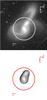 |
Fig. 1 H-band image with the Petrosian radius represented as a white circle (top) and the H-band segmentation map (bottom) with the Petrosian radius represented as a red circle of VV 705. The 2 images have the same FoV. |
Median Gini and M20 values from optical to NIR wavelengths.
5. Results
5.1. Gini and M20 at different Petrosian radius
Given the limitations of the small FoV of the H band, we decided to examine how the two non-parametric coefficients, Gini and M20, vary as a function of the Petrosian radii.
We used the I band as a reference since it has the best angular resolution and it reveals many details and features such as bars, tidal tails, and bright regions. We constructed the final image using four different Petrosian radius (0.67, 1, 1.5, 2) following the same method described earlier, and we measured the Gini and M20 values in the four different segmentation maps.
In Fig. 2, we show that the average Gini-M20 of every morphological class of LIRG changes as the Petrosian radius increases. To check the direction of the Gini-M20 loci of each LIRG as the Petrosian radius increases, we normalize all Gini-M20 values according to the smallest value of Gini and the largest value of M20 in the sample. As a result, all LIRGs have the same point of origin (0, 0) as the radius increases from 0.67 to 2 times the Petrosian value. Figure 2 shows that there is a general trend for the majority of galaxies to increase their Gini and get more negative M20 values for a larger radius. A possible explanation for this result could be the following:
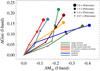 |
Fig. 2 Plot presenting the change in Gini and M20 for various stages of interaction when the radius to calculate the segmentation map increases from 0.67 to 2 times the Petrosian value. ΔGini (and ΔM20) is the difference between the Gini (and M20) at a given radius, minus the value at the smallest radius. The increase in Petrosian radius is indicated by the size of the circles. The seven lines indicate the different morphological classification of LIRGs, based on morphological classification of H11. In particular, sky blue, blue, orange, red, dark red, olive, and green indicate isolated galaxies, separate galaxies (symmetric disks and no tidal tails), progenitor galaxies distinguishable with asymmetric disks or amorphous and/or tidal tails, two nuclei in common envelope, double nuclei plus tidal tail, single or obscured nucleus with long prominent tails and single or obscured nucleus with disturbed central morphology, and short faint tails. |
As the value of the radius increases, pixels with low surface brightness values enter the segmentation map. The influence in the calculation of Gini could be of great importance because, as more fainter pixels enter the segmentation map, the weight of the light distribution becomes more skewed towards the central regions. The behavior of M20 is more complicated. If we increase the radius, the segmentation map would be more extended, and we would expect M20 values to be progressively less negative, closer to zero. However, if the light from the 20% of the brightest pixels comes from a region close to the nucleus, or close to the regions around the two nuclei for double systems, the galaxy as a whole would have a more centrally concentrated light distribution, and the M20 values become increasingly negative.
5.2. Quantifying the morphology of optical and NIR images
In this section, we calculate the Gini and M20 values of our sample in the optical and infrared bands, and study how their position in the Lotz et al. (2004) diagram relates to their morphological classification according to Haan et al. (2011).
Lotz et al. (2004, 2008) divided the Gini-M20 space in three regions for a sample of local galaxies, as well as for a sample of the HST survey of the Extended Groth Strip (EGS) at 0.2 ≤ z ≤ 0.4. These regions identify a galaxy as merger, elliptical (E) or Sa, or disk-like, and Irr.
We expect most of our galaxies to lie in the upper region of the Gini-M20 parametric space because of their merger characteristics (such as tidal tails, double nuclei, and morphologically disturbed structures).
We also examine how the Gini-M20 space is related with M⋆, LIR and SFR. We divide our sample into three bins according to their stellar mass (M⋆), having the same number of galaxies in each bin: (high M⋆ LIRGs: M⋆> 1.52 × 10¹¹M⊙, moderate M⋆ LIRGs: (9.24 × 10¹⁰M⊙<M⋆< 1.52 × 10¹¹M⊙), and small M⋆ LIRGs: M⋆< 9.24 × 10¹⁰M⊙). In addition, we separate the sample as a function of LIR into sub-LIRGs, LIRGs, and ULIRGs. Finally we separate the galaxies based on the SFR into low (<50 M⊙ yr-1 ), moderate (50 <M⊙ yr-1< 100), and high (>100 M⊙ yr-1) SFR.
In Fig. 3 we present the Gini-M20 space as a function of wavelength according to their H11 classification.
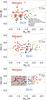 |
Fig. 3 Gini-M20 space in B (top), I (middle) and H band (bottom). Colored filled circles indicate the different morphological classification of LIRGs following H11, where isolated galaxies, separate galaxies (symmetric disks and no tidal tails), progenitor galaxies that are distinguishable with asymmetric disks or amorphous and/or tidal tails, two nuclei in a common envelope, double nuclei plus tidal tail, single or obscured nucleus with long prominent tails, and single or obscured nucleus with disturbed central morphology and short faint tails, respectively. Following Lotz et al. (2004), the upper green solid line separates merger candidates from normal Hubble types while the lower red dotted line divides normal early-types (E/Sa) from late-types (Sb/Irr). The grey rectangle in the H band is the region where ongoing mergers live, regardless of the band. We argue that in the H band, this region can be used to better identify ongoing mergers. |
In Fig. 3, we present the location of our LIRG sample in the Gini-M20 space as a function of wavelength, along with the H11 classification. We see that in the B band, where the light comes from relatively unobscured young and intermediate age stars and star formation regions, 17 galaxies out of 89 of the sample are within the merger locus and none of them is in the region of E/Sa. In the I band, where we expect more evolved stars to contribute to the light, 14 galaxies are above the merger line, but still none of them is in the region of E/Sa. In the NIR, where we can probe structures deeper into the nuclei and the light comes from low-mass main-sequence K stars that are not greatly affected by dust extinction, a few galaxies enter the E/Sa region. We estimate the median values of the two parameters for every band. We identify a trend whereby the median Gini values increase and the median M20 appear to decrease as we move from optical to NIR. Those results are in agreement with the study of Petty et al. (2014), who examined a smaller sample, which also includes UV observations. In addition, the difference between the maximum and the minimum of Gini values decreases while for M20 increases. We show these values in Table 1.
In general, as we characterize the morphology at longer wavelengths from B to H band, we see that isolated or pre-merger galaxies tend to reach more negative M20 values while ongoing mergers tend to lie in the left region. We find that a significant fraction (36%) of the sample do not change their location in the diagram as a function of wavelength and remain in the same region. More than 3/4 (78%) of these LIRGs are double or triple systems that are classified as ongoing mergers and have −0.56 ≥ M20 ≥ −1.55, regardless of the band that we are using to calculate the parameters. The low, nearly constant M20 values are a consequence of the extent of the systems, which clearly show well separated members, regardless of how extended they are individually. This property can be used as a very useful tool to identify galaxies in this particular merger phase, especially in the NIR, where the contamination from systems in other interacting stages is minimal. In other words, galaxies falling in this wedge of the parameter space (see the gray rectangle at the bottom of Fig. 3) are most likely systems that are undergoing an ongoing merger event. The latter result is consistent with Petty et al. (2014) who found that quantitative Gini, M20 measurements do not effectively reflect the wavelength dependence of merging systems. We also separate our sample according to M⋆ and check their positions inside the Gini-M20 plane.
5.3. The Gini and M20 classification at 5.8 μm
In the following, we explore the morphology of our galaxies, as traced by the IRAC 5.8 μm filter. This choice was motivated by the fact that the filter samples both the 6.2 μm polycyclic aromatic feature, which traces star formation, as well as an underlying continuum, which is mostly due to heated dust grains (Smith et al. 2007).
We calculate the non-parametric coefficients at 5.8 μm, following the same method for creating a segmentation map, as in the optical and NIR bands. In this case, we use the MIR image to find the galaxy center and the Petrosian radius. Finally, we construct the segmentation map of every galaxy using two times the Petrosian radius instead of the one Petrosian radius that we used in the previous paragraphs.
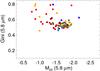 |
Fig. 4 G-M20 non-parametric space of IRAC 5.8 μm. The points are indicated following the colour scheme of Fig. 3 to indicate the morphology classes according to H11. |
Our results, presented in Fig. 4, suggest that most of the galaxies in the sample are grouped in a clump on the Gini-M20 plane with Gini values ~0.5 and −1.5 ≥ M20 ≥ −2.0. The rest are scattered mostly towards the upper left of the plot at higher Gini values. The reason for the clump is mainly due to the ~20 fold decrease in angular resolution of the Spitzer images compared to the HST, which leads to a larger fraction of galaxies having the bulk of their emission originate from an unresolved central source. The remaining galaxies are systems which are either in early stage of interaction or harboring resolved double nuclei, causing their corresponding M20 values to be less negative.
5.4. Luminosity bins of optical and NIR images
It is important to examine how the distribution of our sample in the Gini-M20 space varies according to LIR of galaxies. Since all ULIRGs (LIR> 1012L⊙) in the local Universe are mergers, and therefore display disturbed morphologies (tidal tails, double nuclei, etc.) (Sanders & Mirabel 1996; Farrah et al. 2001; Veilleux et al. 2002; Ishida 2004), we expected all of them would lie above the merger line.
However, Fig. 5 shows that the ULIRGs in our sample have small Gini values and most of them are under the merger line in all bands, which is not consistent with their visual appearance. This rather unexpected result is attributed to the fact that, as we mentioned in Sect. 4.1, we also used the rather small FoV of the H-band images as a reference for the B- and I-band observations. By estimating the Gini and M20 parameters within this region, which correspond to a projected area of 13.4 × 13.4 kpc at the median distance of 145 Mpc for our sample, several of the merging characteristics of the more nearby systems (in particular ULIRGs), such as long tidal tails and bridges, are being suppressed and contribute little to determining the locus of the galaxies in the Gini-M20 plane. This is not the case for more distant systems or cases where double nuclei are clearly visible within the image. This was verified by reevaluating the parameters for the full FoV of the B- and I-band images, which reveals that these galaxies move towards the top left of the plane (see also Petty et al. 2014). Furthermore, Larson et al. (in prep.) also calculated non-parametric coefficients for part of our sample using only the I band and a slightly different methodology in creating the segmentation map. They confirm this trend.
5.5. Morphology and specific SFR
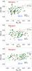 |
Fig. 5 Same as in Fig. 3, but this time the galaxies are grouped by their luminosity. The steel blue crosses indicate sub-LIRGs, the green filled circles LIRGs, and the red triangles ULIRGs. In the B-band, we also show the ULIRG sample with black asterisks that Lotz et al. (2004) used to define the merger region in the Gini-M20 plane. Even though all ULIRGs in our sample are ongoing mergers, they do not appear to populate the corresponding part of the Gini-M20 plane. |
We also examined whether there is a relation between the non-parametric coefficients and the sSFR = (SFR/M⋆). The stellar masses are calculated from IRAC 3.6 μm and 2MASS K-band photometry (Lacey et al. 2008; Howell et al. 2010). For some LIRGs without reliable K-band photometry, the masses are estimated from 3.6 μm data and scaled by the median ratio of (K-band)mass/(3.6 μm)mass from galaxies with measurements in both wavelengths. Our LIRGs have a stellar mass range of 2.54 × 10¹⁰M⊙ < M⋆< 8.15 × 10¹¹M⊙. The calculations of SFR were performed following the equation of Kennicutt (1998) for starburst galaxies, assuming that all LIR comes from reprocessing of star light that the LIR values provided in Díaz-Santos et al. (2013).
The main sequence (MS) of star-forming galaxies indicated by the SFR-M⋆ correlation can be interpreted by the fact that most galaxies spend most of their time producing stars at a normal pace, at least up to z ~ 2 (Elbaz et al. 2007; Daddi et al. 2007; Elbaz et al. 2011). Observations over a wide range of redshifts suggest that the slope of the SFR-M⋆ relation is almost unity, see e.g. (Elbaz et al. 2007; Salmi et al. 2012), which implies that their sSFR does not depend strongly on stellar mass.
In Fig. 6, we show the sSFR as a function of M20 as measured in full ACS B-band maps (see Appendix A), where galaxies have been grouped in luminosity bins. We see that, as LIR increases, the M20 values as well as the sSFR become larger. That is, the B-band emission from ULIRGs, which mostly traces the unobscured stellar populations, appears more extended than in less starbursting galaxies. However, when we investigate the relation between sSFR and M20, as measured using the IRAC 5.8 μm emission, we find the opposite trend (see Fig. 7). Galaxies with higher IR luminosities and sSFR become increasingly compact (show more negative M20 values), in agreement with Elbaz et al. (2011) and Díaz-Santos et al. (2010).
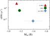 |
Fig. 6 sSFR−M20 in B band. The steel blue cross corresponds to the mean value of the sub-LIRGs sample, the green filled circle indicates the mean value of LIRGs and the red triangle represents the mean value of ULIRGs. The error bars are the standard deviation of the mean values. The larger standard deviation of the sub-LIRG point is due to there being a small number of galaxies (only 8% of the whole sample) in this category. |
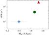 |
Fig. 7 sSFR-M20 in IRAC 5.8 μm. The steel blue crosses correspond to sub-LIRGs, the green filled circles indicate LIRGs and finally the red triangles represent the ULIRGs. The error bars are the standard deviation of the mean values. |
The most likely explanation for the most luminous (U)LIRGs being more extended in the B band, while appearing more compact at 5.8 μm, is the spatial decoupling between the UV/optical and the MIR emission (see also Charmandaris et al. 2004; Howell et al. 2010). In other words, the nuclei of the most compact (U)LIRGs become optically thick and the spatial extent measured in the B (or any optical) band is that of the unattenuated population only. On the other hand, the 5.8 μm probes the dust-reprocessed light from the ongoing starburst and traces the actual spatial distribution of the current star formation. This result confirms that physical sizes of dusty galaxies that are measured in the UV/optical depend highly on the geometry of the dust distribution and can be significantly overestimated. Moreover, this result has a direct application to cosmological surveys of dusty, high redshift galaxies, since the size measurements of these sources mostly come from rest-frame HST UV/optical imaging.
Figure 8 shows the sSFR as a function of the M20 measured in the H band for our sample, binned by stellar mass. We see that more massive galaxies are more extended (i.e., bigger, as would be expected for the same profile, the scaling lengths are larger for the more massive galaxies). The mean M20 values become more negative as the sSFR increases and the mass of the galaxies becomes smaller. Thus, the more massive the LIRG, the more extended the object becomes because the stellar mass is distributed over a larger area.
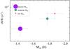 |
Fig. 8 sSFR-M20 in H band. The big purple circle represents the mean value of our sample with large stellar masses (M⋆> 1.52 × 10¹¹M⊙), the intermediate blue circle corresponds to moderate stellar mass (9.24 × 10¹⁰M⊙<M⋆< 1.52 × 10¹¹M⊙) and the small pink circle shows the mean value of small stellar mass (M⋆< 9.24 × 10¹⁰M⊙). The error bars are the standard deviation of the mean values. |
5.6. Dust temperature and non-parametric coefficients
In previous sections, we discussed that LIRGs with larger sSFR appear more compact in the MIR. We also know from Díaz-Santos et al. (2010) that the IR compactness of a galaxy is related to its far-IR colors, and therefore to the averaged dust temperature (Tdust). In this section we explore how Tdust evolves along the merger sequence of LIRGs. We obtain an estimate of the Tdust using the Herschel continuum fluxes of 63 and 158 μm. In particular, we use a modified blackbody function (graybody) as seen in Dupac et al. (2001) (7)where β = 2 and λ0 = 100 μm, to fit the Herschel data, and derive the corresponding dust temperature, which is found in the 26–38 K range.
In Figs. 9 and 10 we plot the FIR flux density ratio f63 μm/f158 μm as a function of the M20 values, while in the right-hand y-axis we also show the equivalent Tdust. Pre-mergers and isolated galaxies have low Tdust values and more negative M20 values. In ongoing mergers, the Tdust increases drastically and the M20 takes higher values (closer to zero), reflecting the separation of the interacting galaxies, in which the starburst has already been triggered. Finally the Tdust in post-merger LIRGs increase slightly as the intensity of the starburst event transitions through the peak of star formation. We find that these results are independent of the waveband used to calculate the M20 statistic.
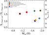 |
Fig. 9 M20 values calculated in the H-band, along with the corresponding Herschel FIR flux density ratios and the estimated Tdust. The sample is grouped by the H11 morphology type, also shown in Fig. 3. The error bars are the standard deviations around the mean of each group. |
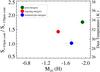 |
Fig. 10 As in Fig. 9, but now merging the H11 classes into three categories: isolated systems or pre-mergers, ongoing mergers, and post mergers. |
6. Discussion
As mentioned earlier, a number of different studies including Lotz et al. (2004), Hung et al. (2014), Petty et al. (2014) and, more recently, Larson et al. (in prep.) used the Gini-M20 space to describe galaxy morphology, based on a variety of samples of local (U)LIRGs. In general, the analysis used in these studies is quite similar. Lotz et al. (2004), Hung et al. (2014), Petty et al. (2014) and Larson et al. (in prep.) create a segmentation map of every galaxy excluding the sky pixels and calculate the non-parametric coefficients inside the map. The major difference between these studies is in the choice of isophotal threshold level used in the calculation of the segmentation map. Lotz et al. (2004) used a value based on the calculation of a Petrosian-like ellipse. Petty et al. (2014) elected to use circular apertures within the NICMOS FoV, ranging between 7.8″ and 15.4″, for all of their images including the UV and optical while Hung et al. (2014) defined the galaxy pixels according to the method of quasi-Petrosian isophote that Abraham et al. (2007) recommended. A novel approach developed by Larson et al. (in prep.) uses the surface brightness of galaxies to create more complex segmentation maps that are well suited for interacting systems with extended morphological structures, and apply the method to a sample of (U)LIRGs in GOALS. For more details, see the above work.
For reasons of consistency, in our analysis, we classified our sample galaxies using the same area in all three Hubble bands, creating segmentation maps based on a circular aperture within one Petrosian radius in each band. As a result, the smaller FoV of the H-band images, combined with the distance to the individual sample galaxy, set an upper limit on the linear scale and physical extent used to determine its morphology. We also calculated Gini and M20 coefficients following the method of quasi-Petrosian isophote (Abraham et al. 2007). We emphasize that we chose to present our results according to the method of one circular Petrosian because the segmentation maps constructed using the quasi-Petrosian isophote method are often contaminated with bright pixels at the edge the maps.
Lotz et al. (2004), who relied only on R-band imagery and defined the segmentation maps in a nearly identical manner to our work, showed that most ULIRGs in the local Universe lie above their defined merger line and are easily identified by their elevated Gini and M20 values. Our results are not as conclusive. We attribute this to the fact that GOALS consists of LIRGs of a diverse morphological type and the smaller FoV, which may miss extended emission from clumps or tails away from the galaxy center. Motivated by Lotz et al. (2004), Lisker (2008) concluded that the Gini coefficient depends strongly on the aperture within which it is computed and this depends strongly on the depth and quality of the images. They also suggested that care needs to be taken with the selection of aperture and limiting magnitude, as well as with the comparison of calculated Gini values to those of other studies. Our measurements fully support this conclusion, as shown in Fig. 2, and the discussion in Sect. 5.1.
Our results are in good agreement with the sub-sample of GOALS studied by Petty et al. (2014), which also included additional UV imagery. Quantitatively, our new values of Gini, M20 are slightly different, but we also find that they do not effectively reflect the wavelength dependence of interacting/merging systems, evident in optical morphology. Merging LIRGs stay in the same general area in the Gini-M20 plane, independent of wavelength. Despite our lack of UV data, we also see that as the observed wavelength increases a large portion of ongoing mergers do not substantially change their locus, even though M20 becomes more negative and the Gini values increase. Petty et al. (2014) have shown that Gini and M20 are useful in identifying merging LIRGs, regardless of rest-frame wavelength at z ~ 0. Our bigger sample reveals that M20 has a larger dynamic range than Gini, and therefore it is more effective in separating LIRGs at different merger stages, in particular in the H band. Hung et al. (2014) also studied the merger fraction in a subsample of GOALS and they found that the level of consistency between Gini-M20 space and a visual classification was 68%. They also stress that LIRGs with disturbed morphology that still have a relatively smooth light distribution (e.g., advanced mergers with no obvious double nuclei) often display low Gini values and tend to be classified as non-interacting systems in the Gini-M20 plane. Our measurements, presented in Sect. 5.2, are in agreement with this finding.
For the analysis of higher-z sources, Conselice et al. (2008) measured galaxy structure and merger fractions in the Hubble Ultra Deep Field (HUDF), adopting a circular aperture of 1.5 Petrosian radius. The Gini values were strongly affected by S/N effects for the majority of their sample. This was also shown in the simulated images of high-z systems using GOALS galaxies by Petty et al. (2014). The influence of low-flux pixels in the calculation of Gini is important because, as more low pixels values enter the segmentation map, the weight of the light distribution becomes more skewed towards the central high pixel value regions. Along the same lines, Kartaltepe et al. (2010) examined the morphological properties of a large sample of 1503 70 μm selected galaxies in the COSMOS field and they suggest that, at z< 1, major mergers contribute significantly to the LIRG population (from 25 to 40%) and clearly dominate for the ULIRG population (from 50 to 80%). A comparison of their visual classification to several automated classification techniques that are commonly used in the literature (including Gini and M20) shows that visual classification is still the most robust method for identifying merger signatures because none of the automated techniques is sensitive to major mergers in all phases. More recently, Cibinel et al. (2015) analyzed HUDF observations, as well as simulated high-z systems, and showed that H-band observations alone are insufficient to trace the morphology/structure of stellar masses at high-z, most probably because of the fact that they correspond to rest-frame optical emission, also confirming that their effectiveness can be strongly affected by low S/N. Moreover, they demonstrate that adding an asymmetry index to the M20 parameter, and measuring them in a mass map, rather than an observed NIR image, can identify mergers with less than 20% contamination from clumpy disks.
7. Conclusions
In this paper we quantify the galaxy morphology of a sample of 89 LIRGs from the GOALS sample observed in the optical, NIR, and MIR, using the non-parametric coefficients Gini and M20. We compare their derived morphology to one that was obtained visually and explore the consistency of the method as a function of a number of physical parameters.
Clearly, our results from the present analysis indicate that simple identification of regions in the Gini-M20 plane as a method to morphologically characterize LIRGs in rather challenging. Several parameters that relate to the rest wavelength emission sampled, depth of the imagery, along with the size of the FoV, can easily lead to misclassification. Revisions to the above methodology, possibly along the lines explored by Larson et al. (in prep.), may provide a more robust approach in the future.
Our analysis suggests that:
-
1.
The Gini and M20 increase in absolute value when the radius that was used to create the corresponding segmentation map increases. The influence in the calculation of Gini is important because, as more pixels with low values enter the segmentation map, the weight of the light distribution is influenced more by the brighter central regions.
-
2.
Comparing the B and I to NIR morphology, we find that the median values of Gini increase while median values of M20 become more negative as the wavelength increases.
-
3.
M20 is a better morphological tracer than Gini, as it can distinguish better systems formed by multiple galaxies from isolated and post-merger LIRGs, and its effectiveness increases with increasing wavelength. In fact, our multi-wavelength analysis allows us to identify a region in the Gini-M20 parameter space where ongoing mergers live, regardless of the band used to calculate the coefficients.
-
4.
We confirm that in the B band, sampling mostly younger stellar populations, as the luminosity of the galaxies increases, they appear more extended and their sSFR increases. Conversely, in MIR, (U)LIRGs are more compact than sub-LIRGs. Moreover, the sSFR is positively correlated with the M20 that is measured in the MIR; – starbursting galaxies appear more compact than normal ones – and it is anti-correlated with it if measured in the B band. We interpret this as evidence of the spatial decoupling between obscured and unobscured star formation, whereby the ultraviolet/optical size of LIRGs that experience an intense central starburst is overestimated owing to higher dust obscuration towards the central regions.
-
5.
The parameters derived from the 5.8μm image do not constrain the morphology well as our sample is grouped into unresolved sources that are concentrated at a given locus of the Gini-M20 plane, while the rest are scattered towards higher Gini and lower M20 values.
-
6.
The estimated temperature of the dust Tdust increases almost monotonically with the merger state of galaxies, while the M20 has a more diverse behavior from isolated galaxies and pre-merger systems (which exhibit more negative M20 values) to ongoing mergers (extended objects) and post-mergers (more compact) regardless of the band.
A review of galaxy classification can be found in Buta (2013).
Acknowledgments
We thank the referee for useful comments on the manuscript. We would also like to thank M. Vika (National Observatory of Athens), E. Vardoulaki (Argelander-Institut fur Astronomie) and K. Larson (Caltech) for many useful discussions and comments on this work. T.D-S. acknowledges support from ALMA-CONICYT project 31130005 and FONDECYT 1151239. A.P. and V.C. would like to acknowledge partial support from the EU FP7 Grant PIRSES-GA-2012-316788.
References
- Abraham, R. G., Valdes, F., Yee, H. K. C., & van den Bergh, S. 1994, ApJ, 432, 75 [NASA ADS] [CrossRef] [Google Scholar]
- Abraham, R. G., van den Bergh, S., Glazebrook, K., et al. 1996, ApJS, 107, 1 [NASA ADS] [CrossRef] [Google Scholar]
- Abraham, R. G., van den Bergh, S., & Nair, P. 2003, ApJ, 588, 218 [NASA ADS] [CrossRef] [Google Scholar]
- Abraham, R. G., Nair, P., McCarthy, P. J., et al. 2007, ApJ, 669, 184 [NASA ADS] [CrossRef] [Google Scholar]
- Allen, P. D., Driver, S. P., Graham, A. W., et al. 2006, MNRAS, 371, 2 [NASA ADS] [CrossRef] [Google Scholar]
- Amiaux, J., Scaramella, R., Mellier, Y., et al. 2012, in SPIE Conf. Ser., 8442 [Google Scholar]
- Armus, L., Mazzarella, J. M., Evans, A. S., et al. 2009, PASP, 121, 559 [NASA ADS] [CrossRef] [Google Scholar]
- Barnes, J. E. 1992, ApJ, 393, 484 [NASA ADS] [CrossRef] [Google Scholar]
- Blain, A. W., Smail, I., Ivison, R. J., Kneib, J.-P., & Frayer, D. T. 2002, Phys. Rep., 369, 111 [NASA ADS] [CrossRef] [Google Scholar]
- Blanton, M. R., Hogg, D. W., Bahcall, N. A., et al. 2003, ApJ, 594, 186 [NASA ADS] [CrossRef] [Google Scholar]
- Buta, R. J. 2013, in Galaxy Morphology, eds. J. Falcón-Barroso, & J. H. Knapen, 155 [Google Scholar]
- Caputi, K. I., Lagache, G., Yan, L., et al. 2007, ApJ, 660, 97 [NASA ADS] [CrossRef] [Google Scholar]
- Chapman, S. C., Blain, A. W., Smail, I., & Ivison, R. J. 2005, ApJ, 622, 772 [NASA ADS] [CrossRef] [Google Scholar]
- Charmandaris, V., Armus, L., Houck, J. R., et al. 2004, BAAS, 36, 702 [NASA ADS] [Google Scholar]
- Cibinel, A., Le Floc’h, E., Perret, V., et al. 2015, ApJ, 805, 181 [NASA ADS] [CrossRef] [Google Scholar]
- Conselice, C. J. 2003, ApJS, 147, 1 [NASA ADS] [CrossRef] [Google Scholar]
- Conselice, C. J. 2014, ARA&A, 52, 291 [NASA ADS] [CrossRef] [Google Scholar]
- Conselice, C. J., Rajgor, S., & Myers, R. 2008, MNRAS, 386, 909 [NASA ADS] [CrossRef] [Google Scholar]
- Daddi, E., Dickinson, M., Morrison, G., et al. 2007, ApJ, 670, 156 [NASA ADS] [CrossRef] [Google Scholar]
- de Vaucouleurs, G. 1959, Handbuch der Physik, 53, 275 [Google Scholar]
- Díaz-Santos, T., Charmandaris, V., Armus, L., et al. 2010, ApJ, 723, 993 [NASA ADS] [CrossRef] [Google Scholar]
- Díaz-Santos, T., Armus, L., Charmandaris, V., et al. 2013, ApJ, 774, 68 [NASA ADS] [CrossRef] [Google Scholar]
- Dickinson, M. 2000, Roy. Soc. Lond. Phil. Trans. Ser. A, 358, 2001 [Google Scholar]
- Dressler, A. 1980, ApJ, 236, 351 [NASA ADS] [CrossRef] [Google Scholar]
- Dupac, X., Giard, M., Bernard, J.-P., et al. 2001, ApJ, 553, 604 [NASA ADS] [CrossRef] [Google Scholar]
- Elbaz, D., Cesarsky, C. J., Chanial, P., et al. 2002, A&A, 384, 848 [NASA ADS] [CrossRef] [EDP Sciences] [Google Scholar]
- Elbaz, D., Daddi, E., Le Borgne, D., et al. 2007, A&A, 468, 33 [NASA ADS] [CrossRef] [EDP Sciences] [Google Scholar]
- Elbaz, D., Dickinson, M., Hwang, H. S., et al. 2011, A&A, 533, A119 [NASA ADS] [CrossRef] [EDP Sciences] [Google Scholar]
- Farrah, D., Rowan-Robinson, M., Oliver, S., et al. 2001, MNRAS, 326, 1333 [NASA ADS] [CrossRef] [Google Scholar]
- Fazio, G. G., Hora, J. L., Allen, L. E., et al. 2004, ApJS, 154, 10 [NASA ADS] [CrossRef] [Google Scholar]
- Frieman, J., & Dark Energy Survey Collaboration 2013, in AAS Meet. Abstr., 221, 335.01 [Google Scholar]
- Gardner, J. P., Mather, J. C., Clampin, M., et al. 2006, Space Sci. Rev., 123, 485 [NASA ADS] [CrossRef] [Google Scholar]
- Graham, A. W., & Driver, S. P. 2005, PASA, 22, 118 [NASA ADS] [CrossRef] [Google Scholar]
- Haan, S., Surace, J. A., Armus, L., et al. 2011, AJ, 141, 100 [NASA ADS] [CrossRef] [Google Scholar]
- Häußler, B., Bamford, S. P., Vika, M., et al. 2013, MNRAS, 430, 330 [NASA ADS] [CrossRef] [Google Scholar]
- Hjorth, J., & Madsen, J. 1991, MNRAS, 253, 703 [NASA ADS] [Google Scholar]
- Hopkins, P. F., Hernquist, L., Cox, T. J., & Kereš, D. 2008, ApJS, 175, 356 [NASA ADS] [CrossRef] [Google Scholar]
- Hopkins, P. F., Cox, T. J., Dutta, S. N., et al. 2009, ApJS, 181, 135 [NASA ADS] [CrossRef] [Google Scholar]
- Howell, J. H., Armus, L., Mazzarella, J. M., et al. 2010, ApJ, 715, 572 [NASA ADS] [CrossRef] [Google Scholar]
- Hubble, E. P. 1926, ApJ, 64, 321 [NASA ADS] [CrossRef] [Google Scholar]
- Hung, C.-L., Sanders, D. B., Casey, C. M., et al. 2014, ApJ, 791, 63 [Google Scholar]
- Ishida, C. M. 2004, Ph.D. Thesis, University of Hawai’i [Google Scholar]
- Kartaltepe, J. S., Sanders, D. B., Le Floc’h, E., et al. 2010, ApJ, 721, 98 [NASA ADS] [CrossRef] [Google Scholar]
- Kennicutt, Jr., R. C. 1998, ARA&A, 36, 189 [Google Scholar]
- Kim, D.-C., Evans, A. S., Vavilkin, T., et al. 2013, ApJ, 768, 102 [Google Scholar]
- Lacey, C. G., Baugh, C. M., Frenk, C. S., et al. 2008, MNRAS, 385, 1155 [NASA ADS] [CrossRef] [Google Scholar]
- Le Floc’h, E., Papovich, C., Dole, H., et al. 2005, ApJ, 632, 169 [NASA ADS] [CrossRef] [Google Scholar]
- Lintott, C., Schawinski, K., Bamford, S., et al. 2011, MNRAS, 410, 166 [NASA ADS] [CrossRef] [Google Scholar]
- Lisker, T. 2008, ApJS, 179, 319 [NASA ADS] [CrossRef] [Google Scholar]
- Lotz, J. M., Primack, J., & Madau, P. 2004, AJ, 128, 163 [NASA ADS] [CrossRef] [Google Scholar]
- Lotz, J. M., Madau, P., Giavalisco, M., Primack, J., & Ferguson, H. C. 2006, ApJ, 636, 592 [NASA ADS] [CrossRef] [Google Scholar]
- Lotz, J. M., Davis, M., Faber, S. M., et al. 2008, ApJ, 672, 177 [NASA ADS] [CrossRef] [Google Scholar]
- LSST Dark Energy Science Collaboration 2012, ArXiv e-prints [arXiv:1211.0310] [Google Scholar]
- Magnelli, B., Elbaz, D., Chary, R. R., et al. 2009, A&A, 496, 57 [NASA ADS] [CrossRef] [EDP Sciences] [Google Scholar]
- Magnelli, B., Popesso, P., Berta, S., et al. 2013, A&A, 553, A132 [NASA ADS] [CrossRef] [EDP Sciences] [Google Scholar]
- Mihos, J. C., & Hernquist, L. 1996, ApJ, 464, 641 [NASA ADS] [CrossRef] [Google Scholar]
- Papovich, C., Dickinson, M., Giavalisco, M., Conselice, C. J., & Ferguson, H. C. 2005, ApJ, 631, 101 [NASA ADS] [CrossRef] [Google Scholar]
- Petrosian, V. 1976, ApJ, 210, L53 [NASA ADS] [CrossRef] [Google Scholar]
- Petty, S. M., Armus, L., Charmandaris, V., et al. 2014, AJ, 148, 111 [NASA ADS] [CrossRef] [Google Scholar]
- Roberts, M. S., & Haynes, M. P. 1994, ARA&A, 32, 115 [NASA ADS] [CrossRef] [Google Scholar]
- Salmi, F., Daddi, E., Elbaz, D., et al. 2012, ApJ, 754, L14 [NASA ADS] [CrossRef] [Google Scholar]
- Sandage, A. 1961, The Hubble atlas of galaxies (Washington: Carnegie Institution) [Google Scholar]
- Sandage, A. 1975, ApJ, 202, 563 [NASA ADS] [CrossRef] [Google Scholar]
- Sandage, A. 2005, ARA&A, 43, 581 [NASA ADS] [CrossRef] [Google Scholar]
- Sanders, D. B., & Mirabel, I. F. 1996, ARA&A, 34, 749 [NASA ADS] [CrossRef] [Google Scholar]
- Sanders, D. B., Mazzarella, J. M., Kim, D.-C., Surace, J. A., & Soifer, B. T. 2003, AJ, 126, 1607 [Google Scholar]
- Schade, D., Lilly, S. J., Crampton, D., et al. 1995, ApJ, 451, L1 [NASA ADS] [CrossRef] [Google Scholar]
- Schutter, A., & Shamir, L. 2015, Astron. Comp., 12, 60 [NASA ADS] [CrossRef] [Google Scholar]
- Sersic, J. L., Pastoriza, M. G., & Carranza, G. J. 1968, Astrophys. Lett., 2, 45 [NASA ADS] [Google Scholar]
- Smith, J. D. T., Draine, B. T., Dale, D. A., et al. 2007, ApJ, 656, 770 [NASA ADS] [CrossRef] [Google Scholar]
- Strateva, I., Ivezić, Ž., Knapp, G. R., et al. 2001, AJ, 122, 1861 [Google Scholar]
- van den Bergh, S., Abraham, R. G., Ellis, R. S., et al. 1996, AJ, 112, 359 [NASA ADS] [CrossRef] [Google Scholar]
- Veilleux, S., Kim, D.-C., & Sanders, D. B. 2002, ApJS, 143, 315 [NASA ADS] [CrossRef] [Google Scholar]
- Williams, R. J., Quadri, R. F., & Franx, M. 2011, ApJ, 738, L25 [NASA ADS] [CrossRef] [Google Scholar]
- Wuyts, S., Förster Schreiber, N. M., van der Wel, A., et al. 2011, ApJ, 742, 96 [NASA ADS] [CrossRef] [Google Scholar]
Appendix A: The Gini and M20 values of the sample in B- and I- field
As we discussed in Sect. 4.1, we present the Gini and M20 values of our sample in the B- and I-band using the original, uncropped ACS maps in their full 0,05′′ per pixel resolution. We construct the segmentation map of each galaxy using the same methodology presented in Sect. 4.1. The only difference is that we defined circular apertures using the brightest pixel in the I-band image (not the H-band image) as the center, and calculate the associated Petrosian radius in both bands. The derived values are presented in Table A.1.
Gini, M20 values of LIRGs in the B- and I-bands using the whole ACS FoV.
Appendix B: Gini and M50
As discussed in the text, the optical and NIR morphologies of LIRGs span the full range – from highly disturbed systems to normal spirals – often having fairly bright star-forming regions at a large distance from the central nucleus. The value of M20 is sensitive in tracing bright regions at the outer parts of the galaxies. For this reason, we wanted to examine if a similar non-parametric coefficient, the M50 could reveal these bright regions even more efficiently. We defined M50 according to Eq. (3), where the limit of σMi is equal to the 50% of the total flux. In Fig. B.1, we present our calculations of G-M50 in the H-band, following the same notation to the one we used in Fig. 3.
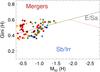 |
Fig. B.1 G-M50 plane of our sample in the H band. The colored filled circles indicate the different morphological classification of LIRGs as described in Fig. 3. |
Comparing these two figures, it is clear that M50 is not as sensitive since the range of values it takes is smaller.
Appendix C: Additional table
Gini, M20 values of LIRGs in the B,I,H, and IRAC 5.8 μm band.
All Tables
All Figures
|
Fig. 1 H-band image with the Petrosian radius represented as a white circle (top) and the H-band segmentation map (bottom) with the Petrosian radius represented as a red circle of VV 705. The 2 images have the same FoV. |
| In the text | |
|
Fig. 2 Plot presenting the change in Gini and M20 for various stages of interaction when the radius to calculate the segmentation map increases from 0.67 to 2 times the Petrosian value. ΔGini (and ΔM20) is the difference between the Gini (and M20) at a given radius, minus the value at the smallest radius. The increase in Petrosian radius is indicated by the size of the circles. The seven lines indicate the different morphological classification of LIRGs, based on morphological classification of H11. In particular, sky blue, blue, orange, red, dark red, olive, and green indicate isolated galaxies, separate galaxies (symmetric disks and no tidal tails), progenitor galaxies distinguishable with asymmetric disks or amorphous and/or tidal tails, two nuclei in common envelope, double nuclei plus tidal tail, single or obscured nucleus with long prominent tails and single or obscured nucleus with disturbed central morphology, and short faint tails. |
| In the text | |
|
Fig. 3 Gini-M20 space in B (top), I (middle) and H band (bottom). Colored filled circles indicate the different morphological classification of LIRGs following H11, where isolated galaxies, separate galaxies (symmetric disks and no tidal tails), progenitor galaxies that are distinguishable with asymmetric disks or amorphous and/or tidal tails, two nuclei in a common envelope, double nuclei plus tidal tail, single or obscured nucleus with long prominent tails, and single or obscured nucleus with disturbed central morphology and short faint tails, respectively. Following Lotz et al. (2004), the upper green solid line separates merger candidates from normal Hubble types while the lower red dotted line divides normal early-types (E/Sa) from late-types (Sb/Irr). The grey rectangle in the H band is the region where ongoing mergers live, regardless of the band. We argue that in the H band, this region can be used to better identify ongoing mergers. |
| In the text | |
|
Fig. 4 G-M20 non-parametric space of IRAC 5.8 μm. The points are indicated following the colour scheme of Fig. 3 to indicate the morphology classes according to H11. |
| In the text | |
|
Fig. 5 Same as in Fig. 3, but this time the galaxies are grouped by their luminosity. The steel blue crosses indicate sub-LIRGs, the green filled circles LIRGs, and the red triangles ULIRGs. In the B-band, we also show the ULIRG sample with black asterisks that Lotz et al. (2004) used to define the merger region in the Gini-M20 plane. Even though all ULIRGs in our sample are ongoing mergers, they do not appear to populate the corresponding part of the Gini-M20 plane. |
| In the text | |
|
Fig. 6 sSFR−M20 in B band. The steel blue cross corresponds to the mean value of the sub-LIRGs sample, the green filled circle indicates the mean value of LIRGs and the red triangle represents the mean value of ULIRGs. The error bars are the standard deviation of the mean values. The larger standard deviation of the sub-LIRG point is due to there being a small number of galaxies (only 8% of the whole sample) in this category. |
| In the text | |
|
Fig. 7 sSFR-M20 in IRAC 5.8 μm. The steel blue crosses correspond to sub-LIRGs, the green filled circles indicate LIRGs and finally the red triangles represent the ULIRGs. The error bars are the standard deviation of the mean values. |
| In the text | |
|
Fig. 8 sSFR-M20 in H band. The big purple circle represents the mean value of our sample with large stellar masses (M⋆> 1.52 × 10¹¹M⊙), the intermediate blue circle corresponds to moderate stellar mass (9.24 × 10¹⁰M⊙<M⋆< 1.52 × 10¹¹M⊙) and the small pink circle shows the mean value of small stellar mass (M⋆< 9.24 × 10¹⁰M⊙). The error bars are the standard deviation of the mean values. |
| In the text | |
|
Fig. 9 M20 values calculated in the H-band, along with the corresponding Herschel FIR flux density ratios and the estimated Tdust. The sample is grouped by the H11 morphology type, also shown in Fig. 3. The error bars are the standard deviations around the mean of each group. |
| In the text | |
|
Fig. 10 As in Fig. 9, but now merging the H11 classes into three categories: isolated systems or pre-mergers, ongoing mergers, and post mergers. |
| In the text | |
|
Fig. B.1 G-M50 plane of our sample in the H band. The colored filled circles indicate the different morphological classification of LIRGs as described in Fig. 3. |
| In the text | |
Current usage metrics show cumulative count of Article Views (full-text article views including HTML views, PDF and ePub downloads, according to the available data) and Abstracts Views on Vision4Press platform.
Data correspond to usage on the plateform after 2015. The current usage metrics is available 48-96 hours after online publication and is updated daily on week days.
Initial download of the metrics may take a while.