© ESO, 2016

1. Introduction

Observations of the Sun at high angular resolution using ground-based telescopes need an accurate modeling of the optical effects induced by atmospheric turbulence. The main problem, however, is the estimation of the optical transfer function (OTF) that describes turbulence effects on recorded images (Labeyrie 1970). Several procedures have been developed a posteriori to observations to calculate the point spread function (PSF) of the whole system atmosphere-instrument or, equivalently, its complex Fourier transform, the OTF. Only the modulus of the OTF, which is the modulation transfer function (MTF), can often be determined or inferred. The MTF gives the contrast reduction of each object frequency induced by both the atmosphere and the telescope. Empirical determination of the PSF or the OTF has been obtained from Mercury or Venus transits (Mattig 1971; Maltby 1971; Maltby & Staveland 1971; Brahde 1982; Wittman & Wohl 1975) or from measurements of the lunar limb over the solar disk during eclipses (Deubner & Mattig 1975; Schmidt et al. 1979; Ricort et al. 1981; Collados & Vasquez 1987; Komm et al. 1990). Normally, Gaussian functions or a combination of Gaussian and Lorentzian functions are used to fit experimental functions. In several cases, atmospheric degradation has been quantified as the effect of an ideal telescope of a given aperture (Deubner & Mattig 1975; Schmidt et al. 1981). Important advances have been achieved in the elaboration of mathematical models to explain the connection between atmospheric turbulence and astronomical image quality. Pioneering works on these subjects are those of Kolmogorov (1941), Chandrashekhar (1952), and Tatarski (1961). The atmosphere is usually considered as an isotropic turbulent medium where an energy spectrum follows Kolmogorov’s law. Two models have been proposed to describe the statistics of the perturbed complex wave. The first is the normal model where phase and amplitude fluctuations have a Gaussian probability function with zero mean value. The second is the log-normal model proposed by Korff (1973), which assumes a Gaussian probability for the fluctuations of both the phase and the logarithm of the amplitude of the incident wave. Fried (1965; 1966) proposed an analytical form of the OTF based on Kolmogorov statistics. This model depends on the Fried parameter r₀, which is defined as the diameter of the equivalent telescope whose spatial resolution results from turbulence effects (Roddier 1981). On the basis of temperature measurements obtained by mean of balloons, Barletti et al. (1977) measured the Fried parameter at several heights. Borgnino and Brandt (1982) measured it using a rotating interferometer (nighttime) and a solar limb meter (daytime). The Fried parameter r₀ has also been estimated from photoelectric measurements of angle-of-arrival (AA) fluctuations at the solar limb (Brandt et al. 1987) and from echosounders and temperature sensors placed on masts (Brandt et al. 1989).

A new theoretical expression of the OTF deduced from the Von Kàrmàn model was established by Conan (2000). This model depends on two optical atmospheric parameters: the Fried parameter r₀ and the spatial coherence outer scale ℒ₀. The knowledge of this last parameter is of major interest in astronomy, mainly for optimizing high angular resolution techniques (speckle interferometry, long baseline interferometry, adaptive optics). Several methods have been proposed to estimate the spatial coherence outer scale ℒ₀ of nighttime observations. Most of them are based on a statistical analysis of the AA-fluctuations (Tallon 1989). A more detailed theoretical study with numerical simulations has led to new techniques that estimate ℒ₀ from its effects on the variance and the covariance of AA-fluctuations (Borgnino 1990; Borgnino et al. 1992; Ziad et al. 1994). A generalized seeing monitor (GSM) was then built (Martin et al. 1994) allowing the evaluation of many astronomical sites (La Silla, Maydanak, Cerro Pachon, Cerro Paranal, etc.) (Martin et al. 2002; Ziad et al. 2000). For daytime observations, ℒ₀ values are still poorly known while their estimations are of great interest in order to evaluate optical effects induced by atmospheric turbulence on solar images. For this reason the solar seeing monitor MISOLFA (Irbah et al. 2010, 2011) was built and installed at the Calern Observatory. It has been in operation since 2011 observing together with the SODISM II experiment dedicated to measuring the solar diameter (Meftah et al. 2013; Irbah et al. 2011). SODISM II is the qualification model of the SODISM telescope flown on board the PICARD space mission launched on 15 June 2010 (Meftah et al. 2014). MISOLFA was designed to provide estimates of the coherence parameters characterizing wavefronts degraded by atmospheric turbulence (Fried’s parameter r₀, size of the isoplanatic patch θ₀, spatial coherence outer scale ℒ₀, and atmospheric correlation times) and also of the optical turbulence profiles (Bouzid et al. 2002). Depending on the requirements, turbulence parameters can be estimated using the MISOLFA focal and/or pupil plane observation modes. The pupil plane observation mode of MISOLFA can be compared to the S-DIMM instrument used for solar observations (Beckers 2001, 2002).

Here we propose a method that can simultaneously estimate the Fried parameter r₀ and the spatial coherence outer scale ℒ₀ for daytime observations. It is based on the comparison between the experimental OTF deduced from solar limb observations and the theoretical expressions obtained from both the Kolmogorov and Von Kàrmàn models. The method estimates the parameters of theoretical OTFs (both r₀ and ℒ₀ for the Von Kàrmàn model and only r₀ for the Kolmogorov model) that best fit the experimental values. This method was previously tested using numerical simulations (Lakhal et al. 2002). We use it in this paper to analyze a set of solar data recorded with MISOLFA in July 2013. We present the results and discuss them using r₀ estimates obtained from AA-fluctuations. In Sect. 2, we recall the needed theoretical models and give, in Sect. 3, a short presentation of MISOLFA and its recorded data. We then explain in Sect. 4 how we estimate atmospheric turbulence parameters and discuss the results.

2. Theoretical models used to estimate turbulence parameters

2.1. Transverse covariance of AA-fluctuations recorded in the focal plane and parameter estimation

The theoretical results presented in this section were obtained in a similar manner to those used to interpret the nighttime observation data given by the GSM experiment (Martin et al. 1994; Ziad et al. 2000). The transverse spatial covariance of the AA-fluctuations observed at a distance B with two telescopes of diameter D is expressed, in the case where the atmospheric turbulence is described by the Von Kàrmàn model, by (Avila et al. 1997) $\begin{array}{ccc}{\mathit{C}}_{\mathit{\alpha }}\mathrm{\left(}\mathit{B}\mathrm{\right)}& \mathrm{=}& \mathrm{0.0716}{\mathit{\lambda }}^{\mathrm{2}}{\mathit{r}}_{\mathrm{0}}^{\mathrm{-}\frac{\mathrm{5}}{\mathrm{3}}}{\mathrm{\int }}_{\mathrm{0}}^{\mathrm{+}\mathrm{\infty }}\mathrm{d}\mathit{f}{\mathit{f}}^{\mathrm{3}}{\left({\mathit{f}}^{\mathrm{2}}\mathrm{+}\frac{\mathrm{1}}{{{\mathrm{ℒ}}_{\mathrm{0}}}^{\mathrm{2}}}\right)}^{\mathrm{-}\frac{\mathrm{11}}{\mathrm{6}}}\\ & & \end{array}$(1)where f is an angular frequency, λ the wavelength, and J₀, J₁, J₂ the Bessel functions of the first kind. The spatial coherence inner scale is taken equal to 0 in the Von Kàrmàn model.

It is easy to deduce the transverse angular covariance by replacing B by θh in Eq. (1) (Bouzid et al. 2002; Seghouani et al. 2002). This means that observations are performed with a single telescope (pupil of diameter D and focal length f_T) in two directions in the sky separated by θ. The parameter h is the altitude of an equivalent impulse layer giving the same optical effects at ground level as the whole turbulent terrestrial atmosphere. This leads to $\begin{array}{ccc}{\mathrm{𝒞}}_{\mathit{\alpha }}\mathrm{\left(}\mathit{\theta }\mathrm{\right)}& \mathrm{=}& \mathrm{0.0716}{\mathit{\lambda }}^{\mathrm{2}}{\mathit{r}}_{\mathrm{0}}^{\mathrm{-}\frac{\mathrm{5}}{\mathrm{3}}}{\mathrm{\int }}_{\mathrm{0}}^{\mathrm{+}\mathrm{\infty }}\mathrm{d}\mathit{f}{\mathit{f}}^{\mathrm{3}}{\left({\mathit{f}}^{\mathrm{2}}\mathrm{+}\frac{\mathrm{1}}{{{\mathrm{ℒ}}_{\mathrm{0}}}^{\mathrm{2}}}\right)}^{\mathrm{-}\frac{\mathrm{11}}{\mathrm{6}}}\\ & & \end{array}$(2)Equation (2) allows us to estimate Fried’s parameter r₀, the spatial coherence outer scale ℒ₀, and the isoplanatic angle θ₀ deduced from the ratio r₀/h using inversion techniques (Seghouani et al. 2002).

In the case of a multilayer turbulent atmosphere, we use the expression of the transverse angular structure function with the assumptions already given. It can be written as $\begin{array}{ccc}{\mathrm{𝒞}}_{\mathit{\alpha }}\mathrm{\left(}\mathit{\theta }\mathrm{\right)}& \mathrm{=}& \mathrm{1.19}{\mathrm{\int }}_{\mathrm{0}}^{\mathrm{+}\mathrm{\infty }}\mathrm{d}\mathit{h}{\mathit{C}}_{\mathit{n}}^{\mathrm{2}}\mathrm{\left(}\mathit{h}\mathrm{\right)}{\mathrm{\int }}_{\mathrm{0}}^{\mathrm{+}\mathrm{\infty }}\mathrm{d}\mathit{f}{\mathit{f}}^{\mathrm{3}}{\left({\mathit{f}}^{\mathrm{2}}\mathrm{+}\frac{\mathrm{1}}{{\mathit{L}}_{\mathrm{0}}\mathrm{(}\mathit{h}{\mathrm{)}}^{\mathrm{2}}}\right)}^{\mathrm{-}\frac{\mathrm{11}}{\mathrm{6}}}\\ & & \end{array}$(3)where ${\mathit{C}}_{\mathit{n}}^{\mathrm{2}}\mathrm{\left(}\mathit{h}\mathrm{\right)}$ is the energy vertical profile of the optical turbulence given by the structure constant for the air refractive index fluctuations, L₀(h) is the turbulent outer scale vertical profile, and ${\mathit{C}}_{\mathit{\alpha }}\mathrm{\left(}\mathrm{0}\mathrm{\right)}\mathrm{=}{\mathit{\sigma }}_{\mathit{\alpha }}^{\mathrm{2}}$ is the AA-fluctuations variance.

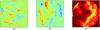Fig. 1 Simulated AA-fluctuations computed directly from the perturbed wavefront phase and observed as intensity fluctuations in the pupil plane image. a) and b) are respectively x and yAA components at the entrance pupil, while c) is the y component observed in the pupil plane image as intensity fluctuations. The perturbed wavefront was simulated in the near-field approximation case considering r0 = 4 cm, ℒ0 = 10 m, and h = 1000 m. The diaphragm width was taken as equal to a few arcseconds.

We can easily relate σ_α to Fried’s parameter in the case of the Kolmogorov model (Borgnino et al. 1982): ${\mathit{r}}_{\mathrm{0}}\mathrm{=}\mathrm{8.25}{\mathrm{10}}^{\mathrm{5}}{\mathit{\lambda }}^{\frac{\mathrm{6}}{\mathrm{5}}}{\mathit{D}}^{\mathrm{-}\frac{\mathrm{1}}{\mathrm{5}}}{{\mathit{\sigma }}_{\mathit{\alpha }}}^{\mathrm{-}\frac{\mathrm{6}}{\mathrm{5}}}\mathrm{\left(}{\mathit{\sigma }}_{\mathit{\alpha }}\mathrm{inarcseconds}\mathrm{\right)}\mathit{.}$(4)The transverse angular structure function is defined by ${\mathit{d}}_{\mathit{\alpha }}\mathrm{\left(}\mathit{\theta }\mathrm{\right)}\mathrm{=}\mathrm{2}\mathrm{[}{\mathit{\sigma }}_{\mathit{\alpha }}^{\mathrm{2}}\mathrm{-}{\mathrm{𝒞}}_{\mathit{\alpha }}\mathrm{(}\mathit{\theta }{\mathrm{\left)}}^{\mathrm{\right]}}\mathit{.}$(5)Introducing Eq. (3) in Eq. (5) leads to $\begin{array}{ccc}{\mathit{d}}_{\mathit{\alpha }}\mathrm{\left(}\mathit{\theta }\mathrm{\right)}& \mathrm{=}& \mathrm{2.4}{\mathrm{\int }}_{\mathrm{0}}^{\mathrm{+}\mathrm{\infty }}\mathrm{d}\mathit{h}{\mathit{C}}_{\mathit{n}}^{\mathrm{2}}\mathrm{\left(}\mathit{h}\mathrm{\right)}{\mathrm{\int }}_{\mathrm{0}}^{\mathrm{+}\mathrm{\infty }}\mathrm{d}\mathit{f}{\mathit{f}}^{\mathrm{3}}{\left({\mathit{f}}^{\mathrm{2}}\mathrm{+}\frac{\mathrm{1}}{{\mathit{L}}_{\mathrm{0}}\mathrm{(}\mathit{h}{\mathrm{)}}^{\mathrm{2}}}\right)}^{\mathrm{-}\frac{\mathrm{11}}{\mathrm{6}}}\\ & & \end{array}$(6)The optical turbulence profile ${\mathit{C}}_{\mathit{n}}^{\mathrm{2}}\mathrm{\left(}\mathit{h}\mathrm{\right)}$ can be estimated from Eq. (6) considering, in a first approach, that L₀(h) = ∞ (Bouzid et al. 2002).

2.2. Estimation of the turbulence parameter using pupil plane observations

The telescope pupil may be imaged with a lens of focal length f_L through a narrow slit D placed in the focal plane on the solar limb. Light rays of the atmospheric perturbed wavefront undergo random angles and pass or not through the diaphragm D. The pupil illumination observed through the diaphragm will then be related to the local slopes of the wavefront. Intensity variations in the pupil plane image are therefore directly related to AA-fluctuations at the telescope entrance pupil when an incoherent extended source is observed. Intensity fluctuations are the summation over the angular field of view allowed by the optical system (i.e., the diaphragm angular size) of all intensity contributions I₀(α,r) of point sources composing the incoherent extended object with luminance O(α) observed in the α angular direction: 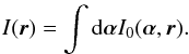$\begin{array}{ccc}\mathit{I}\mathrm{\left(}{r}\mathrm{\right)}\mathrm{=}\mathrm{\int }\mathrm{d}{\alpha }{\mathit{I}}_{\mathrm{0}}\mathrm{\left(}{\alpha }\mathit{,}{r}\mathrm{\right)}\mathit{.}& & \end{array}$A Fourier optics calculation leads to (Borgnino et al. 2007) $\begin{array}{ccc}\mathit{I}\mathrm{\left(}{r}\mathrm{\right)}& \mathrm{=}& {\left(\frac{{\mathit{f}}_{\mathrm{T}}}{{\mathit{f}}_{\mathrm{L}}}\right)}^{\mathrm{2}}\mathrm{\int }\mathrm{\int }\mathrm{\int }\mathrm{d}{\mathit{r}}^{\mathrm{\prime }}\mathrm{d}{\mathit{r}}^{\mathrm{\prime \prime }}\mathrm{d}{\alpha }\mathit{O}\mathrm{\left(}{\alpha }\mathrm{\right)}\exp \left(\mathrm{-}\mathrm{2}\mathit{\pi }\mathrm{i}\frac{{\mathit{r}}^{\mathrm{\prime }}\mathrm{-}{\mathit{r}}^{\mathrm{\prime \prime }}}{\mathit{\lambda }}{\alpha }\right)\\ & & \mathrm{\times }\mathit{t̂}\left(\frac{\mathit{r}\mathrm{-}{\mathit{r}}^{\mathrm{\prime }}}{\mathit{\lambda }{\mathit{f}}_{\mathrm{L}}}\right)\widehat{{\mathit{t}}^{\mathrm{\ast }}}\left(\frac{\mathit{r}\mathrm{-}{\mathit{r}}^{\mathrm{\prime \prime }}}{\mathit{\lambda }{\mathit{f}}_{\mathrm{L}}}\right)\mathit{P}\left(\mathrm{-}{\mathit{r}}^{\mathrm{\prime }}\frac{{\mathit{f}}_{\mathrm{T}}}{{\mathit{f}}_{\mathrm{L}}}\right)\mathit{P}\left(\mathrm{-}{\mathit{r}}^{\mathrm{\prime \prime }}\frac{{\mathit{f}}_{\mathrm{T}}}{{\mathit{f}}_{\mathrm{L}}}\right)\\ & & \mathrm{\times }\mathit{\psi }\left(\mathrm{-}{\mathit{r}}^{\mathrm{\prime }}\frac{{\mathit{f}}_{\mathrm{T}}}{{\mathit{f}}_{\mathrm{L}}}\right){\mathit{\psi }}^{\mathrm{\ast }}\left(\mathrm{-}{\mathit{r}}^{\mathrm{\prime \prime }}\frac{{\mathit{f}}_{\mathrm{T}}}{{\mathit{f}}_{\mathrm{L}}}\right)\mathit{,}\end{array}$(7)where ^ denotes the Fourier transform and ^∗ the conjugation, r(r′,r′′) is a space vector in the pupil plane, λ the wavelength, and t(r) the amplitude transmission of the diaphragm D, P(r) is the pupil function equal to one inside the pupil area and to zero outside, and ψ(r) is the perturbed wavefront with a complex amplitude.

Equation (7) is the basic mathematical model giving the intensity fluctuations in the pupil-image of an incoherent extended object. If the considered object is the solar limb, assuming that its intensity has a linear relationship with ff along the diaphragm length positioned following the x-direction in the instrument focal plane, Eq. (7) leads to (Borgnino et al. 2007) 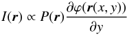$\mathit{I}\mathrm{\left(}{r}\mathrm{\right)}\mathrm{\propto }\mathit{P}\mathrm{\left(}{r}\mathrm{\right)}\frac{\mathit{\partial \varphi }\mathrm{\left(}{r}\mathrm{\right(}\mathit{x,y}\mathrm{\left)}\mathrm{\right)}}{\mathit{\partial y}}$(8)where ϕ(r) is the perturbed wavefront phase at the telescope entrance pupil. The phase derivative fluctuations at each wavefront point correspond to AA-fluctuations. A spatial filtering in pupil image exists due to the diaphragm leading to measure AA-fluctuations in the y-direction. Figure 1 shows intensity fluctuations in the pupil plane image obtained from a numerical simulation. Berdja et al. (2004) have shown that a good linear relationship exists between AA-fluctuations and intensity fluctuations as modeled with Eq. (8) when the solar limb is observed.

We are then able to estimate correlation times of AA-fluctuations if we record intensity fluctuations in the pupil image with a high acquisition rate (typically 1 kHz instead of the commonly used 30 images/second for imaging, see Sect. 4). The spatial coherence parameters r₀ and ℒ₀ may also be obtained together with AA-fluctuation characteristic times. The structure function of AA-fluctuations recorded by means of a pair of photodiodes positioned in the pupil image can be expressed as (Sarazin & Roddier 1990) ${\mathit{d}}_{\mathit{\alpha }}\mathrm{\left(}\mathit{s}\mathrm{\right)}\mathrm{=}\mathrm{0.358}\left[\mathrm{1}\mathrm{-}\mathit{k}{\left(\frac{\mathit{s}}{{\mathit{D}}_{\mathit{p}}}\right)}^{\mathrm{-}\frac{\mathrm{1}}{\mathrm{3}}}\right]{\mathit{\lambda }}^{\mathrm{2}}{{\mathit{r}}_{\mathrm{0}}}^{\mathrm{-}\frac{\mathrm{5}}{\mathrm{3}}}{{\mathit{D}}_{\mathit{p}}}^{\mathrm{-}\frac{\mathrm{1}}{\mathrm{3}}}\mathit{,}$(9)where k is a constant equal to 0.541 or 0.810 depending respectively on whether one considers AA projected on the baseline formed by the photodiodes separated by the distance s or onto a perpendicular direction. The parameter D_p is the diameter of the area integration size of the photodiodes. Equation (9) is used to calculate r₀.

The spatial coherence outer scale ℒ₀ can be deduced from Eq. (2) for θ equal 0. Considering that ℒ₀ is larger than D_p (Ziad et al. 1994), the integration gives ${\mathrm{𝒞}}_{\mathit{\alpha }}\mathrm{\left(}\mathrm{0}\mathit{,}{\mathit{D}}_{\mathit{p}}\mathrm{\right)}\mathrm{=}\mathrm{0.017}{\mathit{\lambda }}^{\mathrm{2}}{{\mathit{r}}_{\mathrm{0}}}^{\mathrm{-}\frac{\mathrm{5}}{\mathrm{3}}}\left[{\mathit{D}}_{\mathit{p}}^{\mathrm{-}\frac{\mathrm{1}}{\mathrm{3}}}\mathrm{-}\mathrm{1.525}{{\mathrm{ℒ}}_{\mathrm{0}}}^{\mathrm{-}\frac{\mathrm{1}}{\mathrm{3}}}\right]\mathit{.}$(10)The ℒ₀ parameter is computed from Eq. (10) considering two photodiodes of different area integration sizes D_p1 and D_p2. It is obtained from the ratio q: $\mathit{q}\mathrm{=}\frac{{\mathrm{𝒞}}_{\mathit{\alpha }}\mathrm{\left(}\mathrm{0}\mathit{,}{{\mathit{D}}_{\mathit{p}}}_{\mathrm{1}}\mathrm{\right)}\mathrm{-}{\mathrm{𝒞}}_{\mathit{\alpha }}\mathrm{\left(}\mathrm{0}\mathit{,}{{\mathit{D}}_{\mathit{p}}}_{\mathrm{2}}\mathrm{\right)}}{{\mathrm{𝒞}}_{\mathit{\alpha }}\mathrm{\left(}\mathrm{0}\mathit{,}{{\mathit{D}}_{\mathit{p}}}_{\mathrm{1}}\mathrm{\right)}}\mathrm{=}\frac{{{{\mathit{D}}_{\mathit{p}}}_{\mathrm{1}}}^{\mathrm{-}\frac{\mathrm{1}}{\mathrm{3}}}\mathrm{-}{{{\mathit{D}}_{\mathit{p}}}_{\mathrm{2}}}^{\mathrm{-}\frac{\mathrm{1}}{\mathrm{3}}}}{{{{\mathit{D}}_{\mathit{p}}}_{\mathrm{1}}}^{\mathrm{-}\frac{\mathrm{1}}{\mathrm{3}}}\mathrm{-}\mathrm{1.525}{{\mathrm{ℒ}}_{\mathrm{0}}}^{\mathrm{-}\frac{\mathrm{1}}{\mathrm{3}}}}\mathrm{·}$(11)

2.3. Turbulence parameter estimation from the OTF

An alternative method exists for estimating Fried’s parameter r₀ and the spatial coherence outer scale ℒ₀ from images recorded in the focal plane. The atmospheric turbulence is seen as random phase aberrations added to the telescope ones. These aberrations have temporal variations and, consequently, the PSF does too. We consider here the temporal average PSF corresponding to long exposure images. It can be written as a linear filtering process over the object frequencies and expressed by 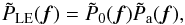$\begin{array}{c}\mathrm{˜}\\ {\mathit{P}}_{\mathrm{LE}}\end{array}\mathrm{\left(}{f}\mathrm{\right)}\mathrm{=}\begin{array}{c}\mathrm{˜}\\ {\mathit{P}}_{\mathrm{0}}\end{array}\mathrm{\left(}{f}\mathrm{\right)}\begin{array}{c}\mathrm{˜}\\ {\mathit{P}}_{\mathrm{a}}\end{array}\mathrm{\left(}{f}\mathrm{\right)}\mathit{,}$(12)where $\begin{array}{c}{}_{\mathrm{˜}}\\ {\mathit{P}}_{\mathrm{0}}\end{array}\mathrm{\left(}{f}\mathrm{\right)}$ is the diffraction-limited OTF of the telescope, which is the pupil autocorrelation function, and $\begin{array}{c}{}_{\mathrm{˜}}\\ {\mathit{P}}_{\mathrm{a}}\end{array}\mathrm{\left(}{f}\mathrm{\right)}$ is the atmospheric transfer function where f denotes a spatial frequency.

The resolution is entirely defined by the atmosphere for large telescopes of good optical quality and the first term can be neglected leading to $\begin{array}{c}{}_{\mathrm{˜}}\\ {\mathit{P}}_{\mathit{LE}}\end{array}\mathrm{\left(}{f}\mathrm{\right)}$ = $\begin{array}{c}{}_{\mathrm{˜}}\\ {\mathit{P}}_{\mathrm{a}}\end{array}\mathrm{\left(}{f}\mathrm{\right)}$. The diffraction-limited OTF $\begin{array}{c}{}_{\mathrm{˜}}\\ {\mathit{P}}_{\mathrm{0}}\end{array}\mathrm{\left(}{f}\mathrm{\right)}$ has to be considered, however, in the case of small telescopes such as MISOLFA. The PSF P_LE is then obtained by inverse Fourier transform from $\begin{array}{c}{\mathrm{˜}}_{}\\ {\mathit{P}}_{\mathit{LE}}\end{array}$. The atmospheric OTF is related to the statistics of the atmospheric phase aberrations φ(r) expressed by the phase structure function D_φ (Roddier 1981), $\begin{array}{c}\mathrm{˜}\\ {\mathit{P}}_{\mathrm{a}}\end{array}\mathrm{\left(}{f}\mathrm{\right)}\mathrm{=}\exp [\mathrm{-}\frac{\mathrm{1}}{\mathrm{2}}{\mathit{D}}_{\mathit{\phi }}\mathrm{\left(}\mathit{\lambda }{f}\mathrm{\right)}]\mathit{,}$(13)where ${\mathit{D}}_{\mathit{\phi }}\mathrm{\left(}{r}\mathrm{\right)}\mathrm{=}\mathrm{⟨}\mathrm{\left[}\mathit{\phi }\mathrm{\right(}{\rho }\mathrm{)}\mathrm{-}\mathit{\phi }\mathrm{(}{\rho }\mathrm{+}{r}\mathrm{)}{\mathrm{]}}^{\mathrm{2}}\mathrm{⟩}\mathit{.}$(14)We note that we pass from the spatial coordinates r in the wavefront plane to the spatial frequencies f in the image plane by multiplying by the wavelength λ. This relation shows that each Fourier component in an image is produced by the interference of light waves separated by a certain distance. It is the principle used in radio and optical interferometers.

2.3.1. Kolmogorov’s model

The model for astronomical seeing initially developed by Tatarski (1961) and then by Fried (1965) is based on Kolmogorov’s work on atmospheric turbulence (1941). It has been reviewed in detail by Roddier (1981). An important result of wavefront propagation through atmospheric turbulence in the case of Kolmogorov’s model is that the structure function D_φ(r) of the wavefront phase perturbations φ(r), on the ground, scales as the separation r to the 5/3 power, ${\mathit{D}}_{\mathit{\phi }}\mathrm{\left(}{r}\mathrm{\right)}\mathrm{=}\mathrm{6.88}(\frac{\mathit{r}}{{\mathit{r}}_{\mathrm{0}}}{)}^{\frac{\mathrm{5}}{\mathrm{3}}}\mathit{,}$(15)where the scaling length r₀ is Fried’s parameter measuring the strength of the magnitude of the seeing. The full width at half maximum (FWHM) of the long exposure PSF when we are limited by the seeing, i.e., for a telescope with diameter much larger than r₀, is obtained from this structure function by $\mathit{FWHM}\mathrm{=}\mathrm{0.98}\frac{\mathit{\lambda }}{{\mathit{r}}_{\mathrm{0}}}\mathit{,}$(16)where λ is the observation wavelength.

The FWHM has a weak dependence on wavelength (λ^{− 1/5}) since r₀ scales as λ^6/5. The typical size of the Fried value for a good observing site is 10 cm at 500 nm, which leads to a resolution (FWHM of the long exposure PSF) of about 1 arcsec. It is important to note that the observed image resolution will be near the value given by Eq. (16) if there are no other contributions coming from other sources such as telescope defocus or tracking errors. For the theoretical Kolmogorov/Tatarski structure function, seeing distortions of the wavefront extend to infinitely large spatial scales. In reality, an upper limit is imposed by the finite thickness of contributing turbulent layers. Hence the 5/3 scaling will apply only to spatial scales smaller than an upper limit known as the outer scale of turbulence ℒ₀ (see Sect. 2.3.2). If the outer scale is not much larger than the telescope aperture diameter, then the image FWHM resolution will be smaller than $\mathrm{0.98}\frac{\mathit{\lambda }}{{\mathit{r}}_{\mathrm{0}}}$, particularly for large wavelength values. We obtain the following expression of the OTF when we insert Eq. (15) into Eq. (13): $\begin{array}{c}\mathrm{˜}\\ {\mathit{P}}_{\mathrm{a}}\end{array}\mathrm{\left(}{f}\mathrm{\right)}\mathrm{=}\exp [\mathrm{-}\mathrm{3.44}(\frac{\mathit{\lambda }\mathit{f}}{{\mathit{r}}_{\mathrm{0}}}{)}^{\mathrm{5}\mathit{/}\mathrm{3}}]\mathrm{·}$(17)Equation (17) allows the OTF calculation in the case of Kolmogorov’s turbulence model. However, Kolmogorov’s model is not well adapted when the effects of the outer scale turbulence become pronounced (Borgnino 2004; Voitsekhovich 1995). This situation appears when the outer scale magnitude is comparable to (or less than) the size of observation zones. Several outer scale dependent models have been suggested for this reason. We consider the Von Kàrmàn model in what follows.

2.3.2. Von Kàrmàn’s model

The phase structure function in the case of the Von Kàrmàn model is given by (Conan 2000; Lakhal et al. 2002) $\begin{array}{ccc}{\mathit{D}}_{\mathit{\phi }}\mathrm{\left(}\mathit{r}\mathrm{\right)}& \mathrm{=}& \frac{\mathrm{\Gamma }\mathrm{(}\mathrm{11}\mathit{/}\mathrm{6}\mathrm{)}}{{\mathrm{2}}^{\mathrm{-}\mathrm{1}\mathit{/}\mathrm{6}}{\mathit{\pi }}^{\mathrm{8}\mathit{/}\mathrm{3}}}[\frac{\mathrm{24}}{\mathrm{5}}\mathrm{\Gamma }\mathrm{(}\mathrm{6}\mathit{/}\mathrm{5}\mathrm{)}{]}^{\mathrm{5}\mathit{/}\mathrm{6}}(\frac{{\mathit{r}}_{\mathrm{0}}}{{\mathrm{ℒ}}_{\mathrm{0}}}{)}^{\mathrm{-}\mathrm{5}\mathit{/}\mathrm{3}}\\ & & \end{array}$(18)where r, r₀, and ℒ₀ are respectively the spatial vector, Fried’s parameter, and the outer scale length of the turbulence; K_ν(r) is the modified Bessel function of the third kind known as the McDonald function; and Γ(s) is the gamma function. The atmospheric OTF of Eq. (13) is then expressed as $\begin{array}{ccc}\begin{array}{c}\mathrm{˜}\\ {\mathit{P}}_{\mathrm{a}}\end{array}\mathrm{\left(}{f}\mathrm{\right)}& \mathrm{=}& \exp \{\mathrm{-}\frac{\mathrm{\Gamma }\mathrm{(}\mathrm{11}\mathit{/}\mathrm{6}\mathrm{)}}{{\mathrm{2}}^{\mathrm{5}\mathit{/}\mathrm{6}}{\mathit{\pi }}^{\mathrm{8}\mathit{/}\mathrm{3}}}[\frac{\mathrm{24}}{\mathrm{5}}\mathrm{\Gamma }\mathrm{(}\mathrm{6}\mathit{/}\mathrm{5}\mathrm{)}{]}^{\mathrm{5}\mathit{/}\mathrm{6}}(\frac{{\mathit{r}}_{\mathrm{0}}}{{\mathrm{ℒ}}_{\mathrm{0}}}{)}^{\mathrm{-}\mathrm{5}\mathit{/}\mathrm{3}}\\ & & \end{array}$(19)Equation (19) contains two terms. The first represents the Kolmogorov case, while the second takes into account the influence of the outer scale. We note that the Von Kàrmàn model is the empirical generalization of the Kolmogorov model for infinite outer scale.

Equations (17) and (19) are used to fit the experimental OTF to estimate Fried’s parameter r₀ and the spatial coherence outer scale ℒ₀.

3. Experimental concept for recording AA-fluctuations by observing the Sun: the seeing monitor MISOLFA

The AA-fluctuations, which are deviations from the normal of the perturbed wavefronts, can be directly observed in image plane (e.g., in Shack-Hartmann’s sensors used in adaptive optics systems). They can also be observed in pupil plane when astronomical sources of interest (the Sun or Moon) present an intensity distribution with a strong discontinuity (Irbah et al. 1993). In this case, an analysis of the perturbed wavefronts analog to a Foucault test is performed. Figure 2 illustrates the principle of the MISOLFA experimental device. The telescope has a pupil size of 25.2 cm and a focal length of 10 m. MISOLFA has two observation modes. The first, the image plane mode, allows direct recording of AA-fluctuations with a CCD camera placed on the solar limb image (No. 1). The observation wavelength is chosen with a filter wheel in the optical beam. A beam splitter allows the creation of the second observation mode, the pupil plane mode, in which the telescope pupil (P1) is observed by means of a lens through a narrow slit placed on the solar limb image (No. 2). The diaphragm size is a few arcseconds wide and about fifty arcseconds long. The pupil image intensity presents fluctuations proportional to AA-fluctuations (see Sect. 2.2). Several photodiodes allow the recording of intensity fluctuations with optical fibers positioned on the image behind diaphragms of different sizes. Signals given by the different photodiodes will be simultaneously recorded and a spatiotemporal analysis performed.

Processing methods are then needed to estimate the atmospheric turbulence parameters from the data recorded with MISOLFA. Hereafter the models described in Sect. 2 are used.

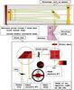Fig. 2 MISOLFA: Experimental design of the monitor.

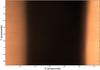Fig. 3 Solar image obtained in the focal plane mode of MISOLFA.

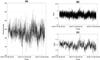Fig. 4 a) Limb positions extracted from MISOLFA solar images, b) intensity fluctuations recorded with the 1 mm photodiode and c) the full intensity (whole pupil) photodiode.

4. Estimating atmospheric turbulence parameters with MISOLFA

This section presents results obtained from solar data recorded with the two observing modes of MISOLFA.

Data from the image plane mode consist of an image series of about 2000 samples recorded at a rate of 30 images per second. Their size is 96 by 128 arcsec. Figure 3 shows an image sample extracted from a data series recorded at 535 nm on 11 August 2011, with this observing mode. The direct and reflected solar limbs shown in the figure are imaged on the CCD thanks to the entrance prism at the front of the telescope (Fig. 2). Each CCD pixel line of the direct and reflected limb images has a direction parallel to the horizon. Angular and spatial fluctuations of AA are obtained from the solar contours extracted from the image series.

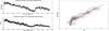Fig. 5 Left curves: Fluctuations of the solar limb positions in image plane (top) and whole image intensity in pupil plane (bottom). Right curve: Relationship between angle (arcseconds) and voltage (volts).

Data of the pupil plane mode come from four photodiodes with different integration areas placed in the 1 cm pupil image: two of them are 0.5 mm in size, and the other two are 1 and 2 mm in size. They correspond respectively to 1.25, 2.5, and 5 cm on the entrance pupil. A fifth photodiode that is 2 mm in size records the intensity fluctuations of the whole pupil image, i.e., 25.2 cm, which is the telescope’s pupil size. All photodiodes deliver their output signal at a rate of 1 kilohertz. Spatio-temporal fluctuations of AA can be then analyzed for each signal or combined photodiode signals.

Solar data were especially recorded on 24 July 2013, in the two MISOLFA observation modes with the aim of calibrating and developing processing methods. The solar images were taken at 610 nm. Figure 4a plots the fluctuations of the mean limb positions extracted from an image series recorded that day. Data of the pupil plane mode were recorded during the same observation period. Figure 4b plots the intensity fluctuations recorded with the photodiode of size 1 mm, while the intensity fluctuations of the whole pupil image are shown in Fig. 4c. A quick look at these curves exhibits some similarities although their temporal sampling is different.

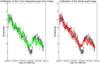Fig. 6 Calibration of pupil intensity fluctuations (see text for details).

4.1. Calibration of intensity fluctuations in pupil plane

Data simultaneously recorded with the two observation modes of MISOLFA were used to validate Eq. (8). This equation links intensity fluctuations in the pupil image to AA-fluctuations and allows photodiode output voltages to be calibrated in angle units. We intentionally let the telescope drift while recording in the two MISOLFA observation modes. We then computed the solar limb positions from the image series and considered intensity fluctuations of the whole pupil image recorded with the appropriate photodiode. In the left panel of Fig. 5 are the plots of the solar limb positions (upper curve) and of the corresponding pupil intensity fluctuations (bottom curve). We observe, as expected, that the corresponding curves have the same trend. We then calibrate the intensity fluctuations expressed in voltage since we know the spatial sampling in the focal plane (0.2 arcsec per pixel). The right panel of Fig. 5 plots solar limb positions versus intensity fluctuations. A linear relationship is clearly observed thereby validating Eq. (8). We use this result to calibrate AA-fluctuations measured in the pupil plane with a high frequency rate thanks to the photodiodes. Figure 6 plots the calibrated AA-fluctuations recorded with the 2 mm photodiode placed in the pupil image (green curve) and the one giving the whole intensity (red curve). The black curve in Fig. 6 corresponds to the temporal positions of the focal solar images recorded at a low frequency rate. The residual difference in low angular positions of the solar limb is due to a bad edge detection when images of the Sun are near the CCD border. The results are nevertheless consistent allowing us to consider the estimation of the turbulence parameters from the pupil data as described in Sect. 2.2. Hereafter we limit the use of the pupil data to the estimation of the correlation time of AA-fluctuations.

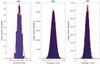Fig. 7 Histogram of AA-fluctuations obtained from an image series recorded 24 July 2013 in image plane mode (a). The same histogram obtained at the same time with the 1 mm (b) and with the full intensity (whole pupil) photodiodes (c) of the pupil plane mode. The red curve is the AA-fluctuations Gaussian fit where R2 is always greater than 0.97.

4.2. Statistics of recorded AA-fluctuations

The statistics of the AA-fluctuations obtained with the MISOLFA observation modes were analyzed first. Some histograms and their Gaussian fits are plotted in Fig. 7. The data used correspond to those shown in Fig. 4. We obtain a Gaussian fit R² greater than 0.97 in each case. This confirms, as expected, that AA-fluctuations have a normal distribution (Roddier 1981) and validates the quality of MISOLFA recorded data. This supposes, however, that observation conditions are comparable, i.e., that there are no additional vibrations due to perturbations of the telescope guiding system induced by winds and/or mechanical problems. We now consider the calibration of pupil data in angle units.

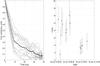Fig. 8 Left: temporal covariance samples of intensity fluctuations (dashed lines) and their mean on the observation period (bold line) obtained with the 1 mm photodiode. Right: some correlation times of AA-fluctuations recorded at Calern Observatory on 24 June 2013.

4.3. Estimation of the correlation time of AA-fluctuations with the pupil data

Data series of the pupil plane mode are used to estimate the correlation time of AA-fluctuations. Intensity fluctuations were recorded at the Calern observatory on 24 June 2013, between 06:00 and 10:30 UT, with the 1 mm photodiode sampled at 1 kilohertz. The covariance of the intensity photodiode signal was computed to evaluate the correlation time. The left panel of Fig. 8 plots covariance samples and the mean curve computed over the observation period. We note that it is not necessary to calibrate intensity fluctuations in angle units before calculating correlation times. We used an equivalent temporal width with the same covariance area to compute the correlation time parameter. We found correlation times of AA-fluctuations ranging from 5 to 16 ms for this specific observation day (Fig. 8, right panel). We observe in this figure that correlation times have a gradual temporal decrease. However, the obtained values are slightly larger than expected (Aime et al. 1981; Lakhal & Irbah 2002). If we look again at the covariance curves in Fig. 8, we note that they have two distinct behaviors. A quick decrease at the origin and, afterwards, another one but slower. A correlation time may then be attributed to each covariance behavior. This was already observed in the temporal statistical analysis of stellar speckle patterns and explained by Aime et al. (1986). A long correlation time is associated with the image motion that translates the whole speckle pattern, and the short one to the speckle lifetime. We are probably faced to the same phenomenon where the pupil image moves in front of the photodiode.

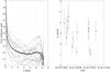Fig. 9 Left: angular covariance samples of AA-fluctuations (dashed lines) and the mean computed over the 24 June 2013 observations (bold line) recorded in image plane mode. Right: some isoplanatic angles of the AA-fluctuations deduced from the covariance curves.

4.4. Estimation of the isoplanatic angle of the AA-fluctuations from image data

We use the solar images recorded the same day in the focal plane mode to estimate the isoplanatic angle of the AA-fluctuations. The obtained results are shown in Fig. 9. The left panel plots some samples of the angular covariance, while the isoplanatic angle values are shown in the right panel. The mean curve of the angular covariance computed over the observation period is also plotted in the figure. As before, no covariance calibration is needed. The isoplanatic angle values range as expected between 1 and 5 arcsec (Irbah et al. 1993).

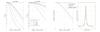Fig. 10 ℒ0 effect on the OTF for typical r0 values (left plots). The ratio between the Von Kàrmàn and Kolmogorov OTF models is used as an illustration. The effect is more significant in the low frequency range (below 0.2 cycles per arcsecond) for small r0 and ℒ0 values. The right plots display an experimental OTF fitted with the two models (left) and the corresponding PSFs (right). Frequencies below 0.2 cycles per arcsecond are considered for the fits since there is more noise at higher frequencies.

4.5. Estimation of the turbulence parameters r₀ and ℒ0 from focal plane observations

Fried’s parameter and the spatial coherence outer scale are estimated for daytime observations with the new method developed in Sect. 2.3 and from AA-fluctuations using both image series recorded in image plane mode. The new method is less sensitive to the telescope guiding system that may perturb the detection of AA-fluctuations. Telescope vibrations and guiding system drifts will affect AA-fluctuations and, consequently, the turbulence parameter estimation in both Kolmogorov and Von Kàrmàn models. This is clearly seen when Fried’s parameter is estimated with Eq. (4), which involves the variance of AA-fluctuations. Our new method uses short-exposure images to calculate long-exposure OTFs or PSFs, which makes it less sensitive to vibrations. In the following, we present the method and then discuss the results.

4.5.1. Calculation of the experimental OTF

The PSF and consequently the OTF can be obtained from the first derivative of the solar limb darkening intensity (Irbah et al. 1993). We add together the columns of the image gradient to calculate the long-exposure OTF from a single image such as the one shown in Fig. 3. First, however, we need to remove the curvature in the solar image. Then we correct the mean from solar limb darkening, otherwise a significant dissymmetry would be introduced. The result of this process leads to the required OTF. First of all, however, a filtering process has to remove noise from the temporal series images while preserving solar limb shape so as not to alter the reconstructed PSF. The filtering we use is based on the compact wavelet analysis and the finite Fourier transform definition (Djafer & Irbah 2012; Djafer et al. 2008). The solar edge defined by the inflexion point of the limb darkening function given by a CCD line is then determined for each cleaned image. Figure 11a shows the cleaned image superposed to its estimated edge and Fig. 11b displays its gradient along the vertical axis (y-axis). A parabolic fit is applied to the set of the edge inflexion points leading to its estimated parameters a, b, and c.

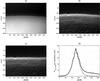Fig. 11 Cleaned image and its edge fitted with a parabola (a pixel is 0.2 arcsec) (a). Image gradient computed along the vertical axis (b) and its correction from the Sun curvature (c). Long-exposure PSF before (full line) and after (dotted line) correction from limb darkening (d).

We proceed as follows to correct the derivative of the cleaned image from curvature effects: if x_i and y_i are the coordinates of the solar edge points in the camera plane, we have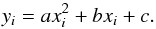${\mathit{y}}_{\mathit{i}}\mathrm{=}\mathit{a}{\mathit{x}}_{\mathit{i}}^{\mathrm{2}}\mathrm{+}\mathit{b}{\mathit{x}}_{\mathit{i}}\mathrm{+}\mathit{c}\mathit{.}$(20)The extrema coordinates (x_s,y_s) of the parabola are given by 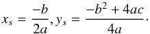${\mathit{x}}_{\mathit{s}}\mathrm{=}\frac{\mathrm{-}\mathit{b}}{\mathrm{2}\mathit{a}}\mathit{,}{\mathit{y}}_{\mathit{s}}\mathrm{=}\frac{\mathrm{-}{\mathit{b}}^{\mathrm{2}}\mathrm{+}\mathrm{4}\mathit{ac}}{\mathrm{4}\mathit{a}}\mathrm{·}$(21)The solar image gradient corrected from the curvature shown in Fig. 11c, is then obtained from 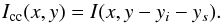${\mathit{I}}_{\mathrm{cc}}\mathrm{\left(}\mathit{x,y}\mathrm{\right)}\mathrm{=}\mathit{I}\mathrm{(}\mathit{x,y}\mathrm{-}{\mathit{y}}_{\mathit{i}}\mathrm{-}{\mathit{y}}_{\mathit{s}}\mathrm{)}\mathit{.}$(22)Under some statistical assumptions such as stationarity and ergodicity, the one-dimensional long-exposure PSF R_LEF(y) according to the Fried definition is obtained by the summation of all columns of I_CC(x,y) corrected for the dissymmetry induced by the solar limb darkening function: ${\mathit{R}}_{\mathrm{LEF}}\mathrm{\left(}\mathit{y}\mathrm{\right)}\mathrm{=}\begin{array}{c}\sum \end{array}{\mathit{I}}_{\mathrm{cc}}\mathrm{\left(}\mathit{x,y}\mathrm{\right)}\mathit{.}$(23)Figure 11d represents this PSF before and after the dissymmetry correction. The OTF is then obtained by (Sanchez et al. 2000) $\begin{array}{c}\mathrm{˜}\\ {\mathit{P}}_{\mathrm{LEF}}\end{array}\mathrm{\left(}{\mathit{f}}_{\mathit{y}}\mathit{,}\mathrm{0}\mathrm{\right)}\mathrm{=}\mathit{FT}\mathrm{\left[}{\mathit{R}}_{\mathrm{LEF}}\mathrm{\right(}\mathit{y}\mathrm{\left)}\mathrm{\right]}$(24)where FT denotes the Fourier transform.

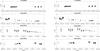Fig. 12 Fried’s parameter obtained with the Von Kàrmàn (left) and Kolmogorov (right) models using data recorded on 17, 24, 26, and 30 July 2013.

4.5.2. Results and discussion

The experimental OTF obtained from the cleaned images is modeled by means of one (Fried’s parameter r₀) or two parameters (r₀ and the spatial coherence outer scale ℒ₀). The ℒ₀ effect on the modeled OTF for typical r₀ daytime values is illustrated by the two curves on the right in Fig. 10. The ratio between the Von Kàrmàn and Kolmogorov OTF models is used to show this effect. We observe that it is more significant in the low spatial frequency range (below 0.2 cycles per arcsecond) when we have small r₀ and ℒ₀ values. These results are expected because the classical model, i.e., the Kolmogorov model, is often not suited for real atmospheric OTFs. This has been observed in other direct and indirect methods (Bell et al. 1999; Dainty & Scaddan 1975; Roddier & Roddier 1973; Bertolotti et al. 1970a,b; Coulman 1969). The Von Kàrmàn model is, in general, better suited to fit the experimental OTF for a wide range of frequency magnitudes. The two right curves in Fig. 10 show an experimental OTF fitted with the two models (left plot) and the corresponding PSFs (right plot). Low spatial frequencies are considered for the model fits since the noise becomes too high over 0.2 cycles per arcsecond. We note, as expected for this frequency range, that the data are close to the profile derived from the two models with, however, a more pronounced difference for the Kolmogorov profile. Hereafter we use the fitting models on the experimental OTFs to estimate the r₀ and ℒ₀ parameters. The left plots of Fig. 13 show some r₀ estimates obtained with image series recorded on 17, 24, and 26 July 2013 with the Kolmogorov and the Von Kàrmàn models. About 15 consecutive solar images are considered in a MISOLFA series to estimate each r₀ value. Each image is first processed and then the OTFs are added.

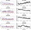Fig. 13 Left curves: Fried’s parameter r0 obtained with the Kolmogorov (black) and Von Kàrmàn (red) models using images recorded on 17, 24, and 26 July 2013. Fried’s parameter r0 obtained with Eq. (4) for the Kolmogorov model is plotted in blue. Right curves: the temporal mean positions of the solar limb leading to r0 estimates from AA-fluctuations using the Kolmogorov model.

We observe that the r₀ values obtained for all series with the two models are relatively stables although they present some differences. Fried’s parameter estimated from AA-fluctuations using Kolmogorov’s model (Eq. (4)) is also computed from some image series of these observation days. We consider for that increasing image number (or acquisition times) in the same data series to compute r₀ values. We are then able to compare them with the values obtained with the new method at the same time. We observe that its value might be overestimated when the length of the image series is not long enough, while the fitting OTF method gives the good values with only a few images (less than half a second). The right plots in Fig. 13 show the temporal mean positions of the solar limb used to compute AA-fluctuation variances needed for the r₀ estimates. These limb positions are deduced from the gradient extrema of the cleaned images (see Sect. 4.5.1). We clearly see some drifts and perturbations that are probably not due to atmospheric turbulence. After this comparative study, we used the OTF method to process more data series recorded with MISOLFA on 17, 24, 26, and 30 July 2013. Figures 12 plot the r₀ values for each of the observation days. Typical r₀ values deduced from the Von Kàrmàn model range from less than half a centimeter to 2.6 cm with a mean value of 1.3 cm over the four observation days. For Kolmogorov’s model, the values are from about 0.5 cm to 4.7 cm with a mean value of 1.5 cm, which is lower than the mean value obtained on the same site using AA-fluctuation variances (Irbah et al. 1994). The error on r₀ is about 10% as we see from its linear approximation in Fig. 15. We note, as expected, that the r₀ values obtained with Von Kàrmàn’s model are lower than the Kolmogorov values. This is due to the ℒ₀ finite values. Indeed, typical ℒ₀ values obtained during these four observation days range between 0.25 and 13 m with a median value over the period of 3.4 m (Fig. 14). Measurement of this parameter is difficult to achieve as evidenced by the significant error affecting it (Fig. 16). However, it reaches a limit value evidenced by the third-order polynomial fit in the figure. These values of ℒ₀ are, nevertheless, in good agreement with the first attempts of Seghouani et al. (2002) and Lakhal et al. (2002) to carry out daytime measurements with solar images not initially intended for this objective. We observe in Fig. 16 that ℒ₀ can have stable temporal values or can present important variations in a few tens of minutes as on 26 July 2013 when it changed from a few meters to less than one in about 30 min. This is clearly shown by the histogram of the four-day ℒ₀ measurements that shows two distinct regimes (left plot in Fig. 17), as was the case for correlation times (see Sect. 4.3). When looking at two specific observation days, we see that we have a normal distribution on 17 July, while this is not the case for 26 July 2013 (right plots in Fig. 17). Observation conditions were highly variable that day as confirmed by the temporal variations of r₀ (Fig. 12). Data dispersions of ℒ₀ have also been observed in nighttime measurements. They were interpreted as transient changes in wavefront spatial structure (Martin et al. 1998). These are the first daytime measurements of the ℒ₀ parameter obtained with MISOLFA that will need to be pursued by considering more observation days.

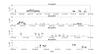Fig. 14 The outer scale parameter ℒ0 obtained using Von Kàrmàn’s model and data recorded on 17, 24, 26, and 30 July 2013.

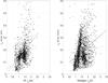Fig. 15 Error on the Fried parameter measurements obtained on 17, 24, 26, and 30 July 2013.

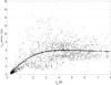Fig. 16 Error on the outer scale parameter measurements obtained on 17, 24, 26, and 30 July 2013.

5. Conclusion

In this paper, we first summarized the theoretical models and basic properties of the solar seeing monitor MISOLFA based at Calern Observatory (France) and already presented in several communication papers, among them Irbah et al. (2010, 2011). We then analyzed some specific observations recorded in July 2013 with the two MISOLFA observation modes. We showed how we used them to calibrate its pupil mode data and we estimated correlation times of the AA-fluctuations. We found that they ranged between 5 and 16 ms and explained why they were slightly larger than expected. We also presented some results on the isoplanatic angle of AA-fluctuations estimated from data recorded with the focal plane mode of MISOLFA. We found values ranging between 1 and 5 arcsec that are in good agreement with already reported results. We then presented a new method for estimating spatial turbulence parameters for daytime observations. It had been developed previously and tested with simulated solar data (Lakhal et al. 2002). It is based on the comparison of the experimental OTF according to Fried’s definition with theoretical models obeying the Kolmogorov and Von Kàrmàn statistics. Fried’s parameter in the case of Kolmogorov’s model, and both Fried’s parameter and the outer scale of turbulence for Von Kàrmàn’s model are estimated from the best fit to the observations in a least squares sense. We applied this method to a set of solar images recorded in July 2013. We also computed the Fried parameter values using AA-fluctuations for Kolmogorov’s model. The comparison revealed that its values may be overestimated if the image series is short. We also showed that they were sensitive to some drift and perturbations probably not due to atmospheric turbulence. Fitted OTFs with the Von Kàrmàn model give more stable values for the Fried parameter. The Von Kàrmàn model is in good agreement with the observations for a wide range of frequency magnitudes. Typical values of r₀ according to Von Kàrmàn ranges from less than 0.5 to 2.6 cm with a mean value of 1.3 cm. For Kolmogorov’s model, values range from 0.5 cm to 4.7 cm with a mean value of 1.5 cm, which is smaller than the mean value obtained on the same site using AA-fluctuation variances. Typical values of ℒ₀ given by the Von Kàrmàn model range from 0.25 to 13 m with a median value of 3.4 m. This parameter value has important variations during short observation times (few tens of minutes) requiring a longer period of data to be analyzed in order to better understand its statistics.

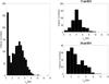Fig. 17 Histograms of measurements of the outer scale parameter ℒ0.

Acknowledgments

Data used for this study have been recorded at Calern Observatory (Observatoire de la Côte d’Azur – France). This work was supported by CNRS (Centre National de la Recherche Scientifique - France) and CNES (Centre National d’Études Spatiales – France).

References

All Figures

Fig. 1 Simulated AA-fluctuations computed directly from the perturbed wavefront phase and observed as intensity fluctuations in the pupil plane image. a) and b) are respectively x and yAA components at the entrance pupil, while c) is the y component observed in the pupil plane image as intensity fluctuations. The perturbed wavefront was simulated in the near-field approximation case considering r0 = 4 cm, ℒ0 = 10 m, and h = 1000 m. The diaphragm width was taken as equal to a few arcseconds.

In the text

	Fig. 2 MISOLFA: Experimental design of the monitor.
In the text

	Fig. 3 Solar image obtained in the focal plane mode of MISOLFA.
In the text

	Fig. 4 a) Limb positions extracted from MISOLFA solar images, b) intensity fluctuations recorded with the 1 mm photodiode and c) the full intensity (whole pupil) photodiode.
In the text

	Fig. 5 Left curves: Fluctuations of the solar limb positions in image plane (top) and whole image intensity in pupil plane (bottom). Right curve: Relationship between angle (arcseconds) and voltage (volts).
In the text

	Fig. 6 Calibration of pupil intensity fluctuations (see text for details).
In the text

	Fig. 7 Histogram of AA-fluctuations obtained from an image series recorded 24 July 2013 in image plane mode (a). The same histogram obtained at the same time with the 1 mm (b) and with the full intensity (whole pupil) photodiodes (c) of the pupil plane mode. The red curve is the AA-fluctuations Gaussian fit where R2 is always greater than 0.97.
In the text

	Fig. 8 Left: temporal covariance samples of intensity fluctuations (dashed lines) and their mean on the observation period (bold line) obtained with the 1 mm photodiode. Right: some correlation times of AA-fluctuations recorded at Calern Observatory on 24 June 2013.
In the text

	Fig. 9 Left: angular covariance samples of AA-fluctuations (dashed lines) and the mean computed over the 24 June 2013 observations (bold line) recorded in image plane mode. Right: some isoplanatic angles of the AA-fluctuations deduced from the covariance curves.
In the text

Fig. 10 ℒ0 effect on the OTF for typical r0 values (left plots). The ratio between the Von Kàrmàn and Kolmogorov OTF models is used as an illustration. The effect is more significant in the low frequency range (below 0.2 cycles per arcsecond) for small r0 and ℒ0 values. The right plots display an experimental OTF fitted with the two models (left) and the corresponding PSFs (right). Frequencies below 0.2 cycles per arcsecond are considered for the fits since there is more noise at higher frequencies.

In the text

	Fig. 11 Cleaned image and its edge fitted with a parabola (a pixel is 0.2 arcsec) (a). Image gradient computed along the vertical axis (b) and its correction from the Sun curvature (c). Long-exposure PSF before (full line) and after (dotted line) correction from limb darkening (d).
In the text

	Fig. 12 Fried’s parameter obtained with the Von Kàrmàn (left) and Kolmogorov (right) models using data recorded on 17, 24, 26, and 30 July 2013.
In the text

	Fig. 13 Left curves: Fried’s parameter r0 obtained with the Kolmogorov (black) and Von Kàrmàn (red) models using images recorded on 17, 24, and 26 July 2013. Fried’s parameter r0 obtained with Eq. (4) for the Kolmogorov model is plotted in blue. Right curves: the temporal mean positions of the solar limb leading to r0 estimates from AA-fluctuations using the Kolmogorov model.
In the text

	Fig. 14 The outer scale parameter ℒ0 obtained using Von Kàrmàn’s model and data recorded on 17, 24, 26, and 30 July 2013.
In the text

	Fig. 15 Error on the Fried parameter measurements obtained on 17, 24, 26, and 30 July 2013.
In the text

	Fig. 16 Error on the outer scale parameter measurements obtained on 17, 24, 26, and 30 July 2013.
In the text

	Fig. 17 Histograms of measurements of the outer scale parameter ℒ0.
In the text

References

- Aime, C., Kadiri, S., Martin, F., & Ricort, G. 1981, Opt. Comm., 39, 287 [NASA ADS] [CrossRef] [Google Scholar]
- Aime, C., Borgnino, J., Martin, F., Petrov, R., & Ricort, G. 1986, J. Opt. Soc. Am., 3, 1001 [NASA ADS] [CrossRef] [Google Scholar]
- Avila, R., Ziad, A., Borgnino, J., et al. 1997, J. Opt. Soc. Amer. A, 14, 11 [Google Scholar]
- Barletti, R., Ceppatelli, G., Paterno, L., Righini, A., & Speroni, N. 1977, Appl. Opt., 16, 2419 [NASA ADS] [CrossRef] [Google Scholar]
- Beckers, J. 2001, Exp. Astron., 12, 1 [NASA ADS] [CrossRef] [Google Scholar]
- Beckers, J. 2002, Astronomical Site Evaluation in the Visible and Radio Range, ASP Conf. Proc., 266, 350 [NASA ADS] [Google Scholar]
- Bell, E. F., Fill, F., & Harvey, J. W. 1999, Sol. Phys., 185, 15 [NASA ADS] [CrossRef] [Google Scholar]
- Berdja, A., Irbah, A., Borgnino, J., & Martin, F. 2004, Proc. SPIE, 5237, 238 [NASA ADS] [CrossRef] [Google Scholar]
- Bertolotti, M., Carneval, M., Muzii, L., & Sette, D. 1970a, Appl. Opt., 9, 510 [NASA ADS] [CrossRef] [Google Scholar]
- Bertolotti, M., Muzii, L., & Sette, D. 1970b, J. Opt. Soc. Am., 60, 1603 [NASA ADS] [CrossRef] [Google Scholar]
- Bouzid, A., Irbah, A., Borgnino, J., & Lantéri, H. 2002, Astronomical Site Evaluation in the Visible and Radio Range, ASP Conf. Proc., 266, 64 [NASA ADS] [Google Scholar]
- Borgnino, J. 1990, Appl. Opt., 29, 1863 [NASA ADS] [CrossRef] [PubMed] [Google Scholar]
- Borgnino, J. 2004, EAS Pub. Ser., 12, 103 [Google Scholar]
- Borgnino, J., & Brandt, P. N. 1982, JOSO Annual Report, 9 [Google Scholar]
- Borgnino, J., Ceppatelli, G., Ricort, G., & Righini, A. 1982, A&A, 107, 333 [NASA ADS] [Google Scholar]
- Borgnino, J., Martin, F., & Ziad, A. 1992, Opt. Comm., 91, 267 [NASA ADS] [CrossRef] [Google Scholar]
- Borgnino, J., Berdja, A., Ziad, A., & Maire, J. 2007, Proc. Symp. Seeing, Kona, Hawaii, 20–22 March, eds. T. Cherubini, & S. Businger [Google Scholar]
- Brahde, R. 1982, Sol. Phys., 26, 318 [Google Scholar]
- Brandt, P. N., Mauter, H. A., & Smartt, R. 1987, A&A, 188, 163 [NASA ADS] [Google Scholar]
- Brandt, P. N., Erasmus, A., Kussoffsky, U., et al. 1989, LEST Techn. Report No. 38 [Google Scholar]
- Chandrashekhar, S. 1952, MNRAS, 112, 475 [NASA ADS] [CrossRef] [Google Scholar]
- Collados, M., & Vasquez, M. 1987, A&A, 180, 223 [NASA ADS] [Google Scholar]
- Conan, R. 2000, Ph.D. Thesis, Nice University, France [Google Scholar]
- Coulman, C. E. 1969, Sol. Phys., 7, 122 [NASA ADS] [CrossRef] [Google Scholar]
- Dainty, J. C., & Scaddan, R. J. 1975, MNRAS, 170, 519 [NASA ADS] [CrossRef] [Google Scholar]
- Deubner, F. L., & Mattig, W. 1975, A&A, 45, 167 [NASA ADS] [Google Scholar]
- Djafer, D., & Irbah, A. 2012, ApJ, 750, 46 [NASA ADS] [CrossRef] [Google Scholar]
- Djafer, D., Thuillier, G., & Sabatino, S. 2008, Sol. Phys., 247, 225 [NASA ADS] [CrossRef] [Google Scholar]
- Fried, D. L. 1965, J. Opt. Soc. Am., 55, 1427 [NASA ADS] [CrossRef] [Google Scholar]
- Fried, D. L. 1966, J. Opt. Soc. Am., 56, 1372 [NASA ADS] [CrossRef] [Google Scholar]
- Irbah, A., Borgnino, J., Laclare, F., & Merlin, G. 1993, A&A, 276, 663 [NASA ADS] [Google Scholar]
- Irbah, A., Laclare, F., Borgnino, J., & Merlin, G. 1994, Sol. Phys., 149,213 [NASA ADS] [CrossRef] [Google Scholar]
- Irbah, A., Corbard, T., Assus, P., et al. 2010, Proc. SPIE, 7735, 77356F [CrossRef] [Google Scholar]
- Irbah, A., Meftah, M., Corbard, T., et al. 2011, Proc. SPIE, 8178, 81780A [CrossRef] [Google Scholar]
- Kolmogorov, A. N. 1941, Turbulence, Classic papers on Statistical Theory. Transl., eds S. K. Friedlander, & L. L. Topper (New York: International Science) [Google Scholar]
- Komm, R., Mattig, W., & Nesis, A. 1990, A&A, 239, 340 [NASA ADS] [Google Scholar]
- Korff, D. 1973, J. Opt. Soc. Am., 63, 971 [NASA ADS] [CrossRef] [Google Scholar]
- Labeyrie, A. 1970, A&A, 6, 85 [NASA ADS] [Google Scholar]
- Lakhal, L., & Irbah, A. 2002, Astronomical Site Evaluation in the Visible and Radio Range, ASP Conf. Proc., 266, 78 [NASA ADS] [Google Scholar]
- Lakhal, L., Irbah, A., Aime, C., Borgnino, J., & Martin, F. 2002, Proc. SPIE, 4538, 112 [NASA ADS] [CrossRef] [Google Scholar]
- Maltby, P., 1971, Sol. Phys., 18, 3 [NASA ADS] [CrossRef] [Google Scholar]
- Maltby, P., & Staveland, L. 1971, Sol. Phys., 18, 443 [NASA ADS] [CrossRef] [Google Scholar]
- Martin, F., Tokovinin, A., Agabi, A., Borgnino, J., & Ziad, A. 1994, Astron. Astrophys. Suppl., 108, 173 [Google Scholar]
- Martin, F., Tokovinin, A., Ziad, A., et al. 1998, A&A, 336, L49 [NASA ADS] [Google Scholar]
- Martin, F., Ziad, A, Conan, C., et al. 2002, Astronomical Site Evaluation in the Visible and Radio Range. ASP Conf. Proc., 266, 138 [NASA ADS] [Google Scholar]
- Mattig, W. 1971, Sol. Phys., 18, 434 [NASA ADS] [CrossRef] [Google Scholar]
- Meftah, M., Corbard, T., Irbah, A., Morand, F., et al. 2013, J. Phys. Conf. Ser., 440 [Google Scholar]
- Meftah, M., Corbard, T., Irbah, A., Morand, F., et al. 2014, Sol. Phys., 289, 1043 [CrossRef] [Google Scholar]
- Ricort, G., Aime, C., Deubner, F., & Mattig, W. 1981, A&A, 97, 114 [NASA ADS] [Google Scholar]
- Roddier, F. 1981, Progress in Optics, 19, 281 [Google Scholar]
- Roddier, C., & Roddier, F. 1973, J. Opt. Soc. Am., 63, 661 [NASA ADS] [CrossRef] [Google Scholar]
- Sanchez Cuberes, M., Bonet, J. A., & Vasquez, M. 2000, ApJ, 538, 940 [NASA ADS] [CrossRef] [Google Scholar]
- Sarazin, M., & Roddier, F. 1990, A&A, 227, 294 [NASA ADS] [Google Scholar]
- Schmidt, W., Deubner, F. L., Mattig, W., & Mehltretter, J. P. 1979, A&A, 75, 223 [NASA ADS] [Google Scholar]
- Schmidt, W., Knolker, M., & Schroter, E. H. 1981, Sol. Phys., 73, 217 [NASA ADS] [CrossRef] [Google Scholar]
- Seghouani, N., Irbah, A., & Borgnino. 2002, Astronomical Site Evaluation in the Visible and Radio Range, ASP Conf. Proc., 36 [Google Scholar]
- Tallon, M. 1989, Ph.D. Thesis, Nice University, France [Google Scholar]
- Tatarski, V. I. 1961, Wave Propagation in a Turbulente Medium (New York: McGraw-Hill) [Google Scholar]
- Voitsekhovich, V. 1995, J. Opt. Soc. Am., 12, 2194 [NASA ADS] [CrossRef] [Google Scholar]
- Wittman, A., & Wohl, H. 1975, Sol. Phys., 44, 231 [NASA ADS] [CrossRef] [Google Scholar]
- Ziad, A., Borgnino, J., Martin, F., & Agabi, A. 1994, A&A, 282, 1021 [NASA ADS] [Google Scholar]
- Ziad, A., Conan, C., Tokovinin, A., Martin, F., & Borgnino, J. 2000, Appl. Opt., 39, 5415 [NASA ADS] [CrossRef] [PubMed] [Google Scholar]