| Issue |
A&A
Volume 591, July 2016
|
|
|---|---|---|
| Article Number | A11 | |
| Number of page(s) | 16 | |
| Section | Galactic structure, stellar clusters and populations | |
| DOI | https://doi.org/10.1051/0004-6361/201527558 | |
| Published online | 02 June 2016 | |
SMC west halo: a slice of the galaxy that is being tidally stripped?
Star clusters trace age and metallicity gradients⋆,⋆⋆
1 European Southern Observatory, Alonso de Córdova 3107, Santiago, Chile
e-mail: bdias@eso.org
2 Instituto de Astronomia, Geofísica e Ciências Atmosféricas, Universidade de São Paulo, Rua do Matão 1226, Cidade Universitária, 05508-900 São Paulo, Brazil
3 Laboratório de Astrofísica Teórica e Observacional, Departamento de Ciências Exatas e Tecnológicas, Universidade Estadual de Santa Cruz, Rodovia Jorge Amado km 16, 45662-000 Ilhéus, Bahia, Brazil
4 Universidade Federal do Rio Grande do Sul, IF, CP 15051, 91501-970 Porto Alegre, RS, Brazil
5 Dipartimento di Fisica e Astronomia Galileo Galilei, University of Padova, vicolo dell’Osservatorio 3, 35122 Padova, Italy
6 INAF–Osservatorio Astronomico di Padova, Vicolo dell’Osservatorio 5, 35122 Padova, Italy
Received: 14 October 2015
Accepted: 10 April 2016
Context. The evolution and structure of the Magellanic Clouds is currently under debate. The classical scenario in which both the Large and Small Magellanic Clouds (LMC, SMC) are orbiting the Milky Way has been challenged by an alternative in which the LMC and SMC are in their first close passage to our Galaxy. The clouds are close enough to us to allow spatially resolved observation of their stars, and detailed studies of stellar populations in the galaxies are expected to be able to constrain the proposed scenarios. In particular, the west halo (WH) of the SMC was recently characterized with radial trends in age and metallicity that indicate tidal disruption.
Aims. We intend to increase the sample of star clusters in the west halo of the SMC with homogeneous age, metallicity, and distance derivations to allow a better determination of age and metallicity gradients in this region. Positions are compared with the orbital plane of the SMC from models.
Methods. Comparisons of observed and synthetic V(B−V) colour-magnitude diagrams were used to derive age, metallicity, distance, and reddening for star clusters in the SMC west halo. Observations were carried out using the 4.1 m SOAR telescope. Photometric completeness was determined through artificial star tests, and the members were selected by statistical comparison with a control field.
Results. We derived an age of 1.23 ± 0.07 Gyr and [Fe/H] = −0.87 ± 0.07 for the reference cluster NGC 152, compatible with literature parameters. Age and metallicity gradients are confirmed in the WH: 2.6 ± 0.6 Gyr/° and −0.19 ± 0.09 dex/°, respectively. The age-metallicity relation for the WH has a low dispersion in metallicity and is compatible with a burst model of chemical enrichment. All WH clusters seem to follow the same stellar distribution predicted by dynamical models, with the exception of AM-3, which should belong to the counter-bridge. Brück 6 is the youngest cluster in our sample. It is only 130 ± 40 Myr old and may have been formed during the tidal interaction of SMC-LMC that created the WH and the Magellanic bridge.
Conclusions. We suggest that it is crucial to split the SMC cluster population into groups: main body, wing and bridge, counter-bridge, and WH. This is the way to analyse the complex star formation and dynamical history of our neighbour. In particular, we show that the WH has clear age and metallicity gradients and an age-metallicity relation that is also compatible with the dynamical model that claims a tidal influence of the LMC on the SMC.
Key words: galaxies: star clusters: general / Magellanic Clouds / galaxies: structure / Hertzsprung-Russell and C-M diagrams / galaxies: stellar content
Based on observations obtained at the Southern Astrophysical Research (SOAR) telescope, which is a joint project of the Ministério da Ciência, Tecnologia, e Inovação (MCTI) da República Federativa do Brasil, the US National Optical Astronomy Observatory (NOAO), the University of North Carolina at Chapel Hill (UNC), and Michigan State University (MSU).
Tables of photometry are only available at the CDS via anonymous ftp to cdsarc.u-strasbg.fr (130.79.128.5) or via http://cdsarc.u-strasbg.fr/viz-bin/qcat?J/A+A/591/A11
© ESO, 2016
1. Introduction
Hierarchical accretion of dwarf galaxies is the most likely origin of stellar halos in large spiral galaxies such as the Milky Way (MW), as predicted by Λ-cold dark matter (ΛCDM) models, and early work by Searle & Zinn (1978). Local Group galaxies are a suitable laboratory in which to study cosmology in very much detail by examining the interactions between the Milky Way and its satellites, in particular the Magellanic Clouds. The Large and Small Magellanic Clouds (LMC and SMC) are the core of a complex system of gas streams with stellar counterparts in some cases. They have an irregular shape, and complex star formation and chemical enrichment histories. They are currently on a close passage to the Milky Way, but there is no agreement in the literature whether they are orbiting our Galaxy periodically (e.g. Diaz & Bekki 2012) or if this is their first close encounter (e.g. Besla et al. 2007). It is likewise debated whether the streams were caused by the Milky Way influence or only by the two Magellanic Clouds themselves (e.g. Nidever et al. 2008).
Since Mathewson et al. (1974) detected the trailing gas structure called Magellanic stream, which indicates that both the LMC and SMC are on a polar orbit around the Milky Way, many different approaches have been implemented to understand their history. The two most reasonable explanations would be ram pressure stripping by an ionized gas in the Milky Way halo (e.g. Moore & Davis 1994) or tidal stripping caused by a close encounter of the clouds and the Milky Way about 1.5 Gyr ago (e.g. Gardiner & Noguchi 1996). Putman et al. (1998) ruled out the MW ram pressure model by finding a leading arm of gas that is evidence in favour of MW tidal stripping.
The new open question that is under debate in the literature is whether the current passage of the SMC and LMC very close to the Milky Way is the first (e.g. Besla et al. 2007, 2010) or if they have a quasi-periodic orbit around our Galaxy (e.g. Gardiner & Noguchi 1996). Besla et al. (2007) supported a first encounter of the LMC and SMC with the Milky Way now, arguing that the SMC and LMC have entered the MW dark matter halo about 3 Gyr ago and that the shock of encountering the MW halo gas has triggered the recent star formation. The authors explained the formation of the Magellanic stream 4 Gyr ago by the interaction of the SMC and LMC with each other and without any MW influence or a stellar counterpart. Diaz & Bekki (2012) instead suggested that the SMC and LMC are orbiting the Milky Way with a period of about 2 Gyr, arguing that this better reproduces the observed positions and velocities for the SMC. In this case, star formation would be triggered by the tidal forces of the MW, and there would be stellar counterparts of the gas structures. Both scenarios are limited to morphology and kinematics and have their advantages and drawbacks, but the deadlock of the discussion might be solved with proper motions of the clouds (e.g. Kallivayalil et al. 2013, using a space-based telescope; Vieira et al. 2010, using a ground-based telescope).
Close encounters of SMC and LMC, or between SMC and LMC and the Milky Way, would trigger star formation. This means that stellar populations are very important to understand the interaction timescales of the galaxies. To separate this intricate scenario for the Magellanic Cloud evolution during the past decade, significant efforts have been made in terms of deriving the star formation rate SFR(t), age-metallicity relation (AMR), and age and metallicity gradients using field stars and stellar clusters. For the SMC, several photometric works have recovered the SFR(t) and/or AMR by means of colour-magnitude diagram (CMD) analyses. We recall the works that were based on very deep and small HST fields (e.g. Chiosi & Vallenari 2007; Cignoni et al. 2013; Weisz et al. 2013), and on shallower large surveys in the visible (e.g. Harris & Zaritsky 2004; Noël et al. 2009; Piatti 2012b, 2015) and in the near-infrared, such as the VISTA Survey for the Magellanic Clouds (VMC; Cioni et al. 2011; Rubele et al. 2015). This last survey was specifically designed to reach faint main-sequence turnoffs of the oldest clusters for 170 deg2 in the LMC, SMC, bridge, and stream, taking the advantage that light in the near-infrared region is almost unaffected by dust.
Spectroscopical studies in the near-infrared involving the CaII triplet of red giant stars (Carrera et al. 2008; Dobbie et al. 2014) or high-resolution optical spectra (Mucciarelli 2014) have yielded fundamental results for AMR, the metallicity distribution, and metallicity gradient for the SMC. These photometric and spectroscopic works have concluded the following: The SMC had an initial period of low star formation rate for ages older than 10 Gyr. At least two periods of enhanced SFR followed at intermediate ages, the first around 5−8 Gyr ago, the second about 1−3 Gyr ago. These might have been associated with close encounters with the LMC or MW. Several bursts of star formation in the last 500 Myr form a complex spatial pattern. The metallicities of field stars are systematically lower than those of their LMC and MW counterparts. The AMR is space dependent and presents a significant spread in metallicity for intermediate ages (1−8 Gyr). An age gradient is formed by the young stars that are concentrated in the SMC bar and the old stars that form a larger and smoother ellipsoidal structure. Finally, the spectroscopic results indicate a metallicity gradient, but this is not consensus in the photometric works.
Additionally, the main episodes of star formation have been confirmed by the results for stellar clusters from the analysis of CMDs using the HST (e.g. Glatt et al. 2008a,b; Girardi et al. 2013), the VLT (Parisi et al. 2014), and 4 m class telescopes (Piatti et al. 2005b, 2007b, 2011; Piatti 2011a,b; Dias et al. 2014), as well as CaII triplet spectroscopy (Parisi et al. 2009, 2015). These analyses also showed how difficult it is to assign a unique AMR because the metallicity for a given age is highly dispersed. On the other hand, these works revealed no strong evidence of a metallicity radial gradient. Furthermore, the metallicity distribution presented by Parisi et al. (2015) is clearly bimodal, with peaks at [Fe/H] = −1.1 and −0.8 dex. This result do not find a counterpart in the field stars, as demonstrated by the analysis of ~3000 red giant stars performed by Dobbie et al. (2014), who found a single peak at [Fe/H] ~ −1.0. Equally challenging, the global AMR for both field and cluster stars does not present a narrow distribution in favour of a single chemical evolution model, which suggests multiple events during the SFH of the SMC.
The SMC complexity is also imprinted on its three-dimensional structure. The distribution of SMC red giant branch (RGB) stars does not present any sign of rotation (Harris & Zaritsky 2006), which is the case for the HI component (Stanimirović et al. 2004). These results suggest that the stellar component follows a spheroidal distribution, whereas the gas is rotating in a disc-like structure. Furthermore, the SMC presents a significant line-of-sight depth, ranging from ~6−14 kpc in the inner parts (Crowl et al. 2001; Subramanian & Subramaniam 2012) to ~23 kpc in the eastern parts along the Magellanic bridge (Nidever et al. 2013). It is possible to find stars ~12 kpc closer than the bulk of SMC stars in the direction of the bridge. Bica et al. (2015) derived even shorter distances to stellar clusters in the Magellanic bridge, raising the possibility that they are part of a tidal dwarf galaxy in formation.
The SMC has been shown to have complex structures and an involved history. We therefore study this galaxies in separate parts in this paper. Considering ellipses instead of circumferences to draw cluster distances to the SMC centre is a better choice for this galaxy shape, as proposed by Piatti et al. (2005a). This is shown in Fig. 1. This system allows us to divide the clusters into an internal (a< 2°) and an external (a > 2°) group. The second group is more interesting because it tells the tidal history of the SMC as recorded by star clusters. Finding age and/or metallicity gradients in the external group is a good indicator of tidal structures, but all the clusters together show a high dispersion and no clear gradient (see Fig. 10). This is not the case when the external group is separated according to the different gas structures. In particular, the western clusters (called west halo, hereafter WH) indicate some gradient in age and possibly in metallicity (Dias et al. 2014, hereafter Paper I). The WH does not correspond to any named gas structure, it is located in the wing and bridge direction, but on the opposite side. The best way to characterize the possible age and metallicity gradients is to analyse the different groups in a homogeneous way.
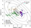 |
Fig. 1 Distribution of SMC star clusters as catalogued by Bica et al. (2008). Ellipses represent the distances from the SMC centre, as defined in Paper I. The different groups main body, wing and bridge, counter-bridge, and west halo are clearly identified as grey dots, green triangles, yellow squares, and blue diamonds. West halo clusters analysed in this work are highlighted with large red triangles, and those analysed in Paper I are displayed as large cyan circles. |
West halo clusters with known parameters, selected as a subsample of Bica et al. (2008) using our definition.
In Sect. 2 the photometric data and reductions are presented. In Sect. 3 the method of isochrone fitting is described. The results are reported in Sect. 4. Conclusions are drawn in Sect. 5.
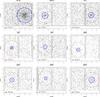 |
Fig. 2 Sky maps of all nine clusters. All plots have the same contrast scale for magnitudes to allow a fair visual comparison. Blue circles indicate the adopted cluster size based on the catalogue of Bica et al. (2008) that were increased in some cases to include more stars for the statistical field-star decontamination. Red circles are the smallest limit around the cluster considered to select field stars, which has a radius of 2.5′ for NGC 152, and 1.5′ for the others. The values are provided in Table 4. |
2. Data
2.1. Selection of targets and observations
The definition of the WH region is based on the ellipses centred on the SMC centre (PA = 45°, e = 0.87), as shown in Fig. 1. All clusters located beyond a> 2° and relative α· cosδ< −1° are selected as WH clusters. The catalogue of Bica et al. (2008) lists 31 clusters in this region. Only 15 of these have at least age and metallicities available in the literature, mostly using CMD analysis. They are listed in Table 1. The remaining 16 clusters, which are fainter, have no dedicated studies so far. We observed 9 of them that are spread through the extension of the WH. This increased the statistics of stellar clusters with no parameters in this region from 15 to 24 clusters (44% to 77%) and offers the possibility of establishing gradients in age and metallicity, as previously suggested in Paper I. We included NGC 152 as a reference cluster, compared with the CMD analysis by Rich et al. (2000) and Correnti et al. (in prep.), both using HST images. The conversion of magnitudes from the HST to the Johnson system may have been problematic in Rich et al. (2000) because the CMDs of NGC 411 and NGC 419 have different colours (see their Fig.1), while Girardi et al. (2013) showed that they are similar. Moreover, Correnti et al. have a deeper CMD with lower photometric errors, but in different bands than those we use in this work. We later compare our results with those from both works, but with some reservation with respect to the results of Rich et al.
In Fig. 1 we also define wing and bridge clusters as all objects located beyond a> 2°, relative α·cosδ> −1° and relative δ< 0.8°. They are located in the region that was originally defined as the SMC wing by Shapley (1940), which extends towards the LMC. The other external group is the counter-bridge, located beyond a> 2°, relative α·cosδ> −1° and relative δ> 0.8°. These clusters are in the region that was defined by Besla (2011) and Diaz & Bekki (2012) as the counterpart of the bridge.
Optical images of the SMC WH clusters were obtained using the SOAR Optical Imager (SOI) in the 4.1 m Southern Astrophysical Research (SOAR) telescope, under the project SO2013B-019 using the same setup as in Paper I. B and V filters were used to detect stars in the magnitude range 16 <V< 24, which covers all required CMD features to derive age, metallicity, distance, and reddening, that is, a few magnitudes below the main-sequence turnoff (MSTO) and few magnitudes above the red clump (RC). While the MSTO is a crucial CMD feature to determine age, the RC and the red giant branch (RGB) are particularly important to constrain distance and metallicity. SOI/SOAR has a field of view of 5.26′ × 5.26′ and is composed of two CCDs that are separated by gap of 7.8″. Because of the gap, we centred the clusters in the centre of one of the CCDs to avoid losing important information on the cluster. The sky maps of all observed clusters show their positions in the SOI FOV in Fig. 2. The pixel scale of 0.077″/pixel was converted into 0.154″/pixel because we used a setup of 2 × 2 binned pixels. Observations were carried out during two nights, the first had poor seeing (1.5−2.0″) , the second good seeing (0.8−1.2″). The only cluster good enough from the first night is Kron 11, all other eight clusters analysed in this work were observed in the second night. The observation log is presented in Table 2.
2.2. Data reduction and photometry
The data were reduced with dedicated SOAR/IRAF packages1 to properly handle the SOI mosaic images. Aperture and PSF photometry were performed using the DAOPHOT/IRAF package (Stetson 1987). Photometric errors are displayed in Fig. 3 for the reference cluster NGC 152 as an example, a similar plot for all clusters is presented in Appendix A. Some of these plots show two stripes for a given set of stars, for example the bottom panel of Fig. 3. Each stripe corresponds to one of the two chips of the instrument (as shown in Fig. 2). The difference of the photometric errors between the two chips is very small and larger for fainter stars, which does not affect the analysis in this paper.
The same fields of standard stars as were used in Paper I were observed here. We used the selection of Sharpee et al. (2002). However, instead of using only a few reference stars listed in Sharpee et al. (2002), we matched all stars in the fields with the stars in the Magellanic Clouds Photometric Survey by Zaritsky et al. (2002, MCPS). Only bright stars with V< 17.5 (above the red clump) were considered, which avoids most of possible variable stars in the field and guarantees smaller photometric errors. We also excluded outliers with large errors from MCPS sample. Using MCPS magnitudes as references, we fitted Eq. (1) to find the zero point β and colour coefficient α:  (1)where M corresponds to either B or V, and m corresponds to the respective instrumental magnitudes (given by −2.5 × log(counts/exptime) already corrected by airmass effects). Airmass coefficients used to correct the magnitudes were 0.22 ± 0.03 mag/airmass and 0.14 ± 0.03 mag/airmass for the B and V-bands, respectively (as can be found at the CTIO website2). Using the residuals of the fit, we made three 1σ clippings to exclude outliers and selected a narrow distribution of well-behaved stars in a range of colours of −0.3 < (B−V) < 2.0. The final fitting is displayed in Fig. 4 for filters B and V, with the respective residual plots. Fitted coefficients are listed in Table 3 together with quality factors r2 and σ.
Observation log.
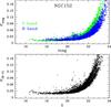 |
Fig. 3 Photometric errors from IRAF for the reference cluster NGC 152 in bands B and V, and colour B−V. |
2.3. Photometric completeness and cluster membership
Artificial star tests (ASTs) were made using the task addstar in IRAF and additional scripts to determine photometric completeness. We generated stars with magnitudes 17 <V< 23 in steps of 0.25 mag to cover all features in the CMD of target clusters. We randomly chose V magnitudes within each interval of magnitude and distributed the stars in radial symmetry around the cluster centre. We verified that the smallest distance between any pair of stars was ≳3.5· ⟨ FWHM ⟩ to avoid introducing artificial crowding (e.g. Paper I; Rubele et al. 2011). For NGC 152 we generated 2301 stars for each magnitude bin within a radius of 1.8′ and 467 stars for the other clusters within 0.8′ around the cluster centre. To calculate B magnitudes for these stars that were to be used to include artificial stars in the B-band images, we tried to follow approximate colours of the CMD structures for each cluster and applied this difference to the V magnitudes, keeping the same positions as were calculated for V images. For each magnitude bin of 0.25 mag we introduced artificial stars as described above in B and V-bands for a given cluster and performed the photometry and calibration exactly as was done before for the cluster. After this, we counted the percentage of recovered artificial stars. For each magnitude bin we repeated this procedure twice to obtain different random positions for the artificial stars and avoid biases. In Fig. 5 we show the completeness curves for the reference cluster NGC 152 for different radii and V magnitudes; the curves for the other clusters are presented in Appendix A.
Cluster member stars were estimated statistically following the method of Paper I developed by Kerber & Santiago (2005). The idea is to compare the CMD of stars in the direction of the cluster with another made of nearby field stars. For each bin in colour and magnitude the number of stars in the two CMDs are counted and normalized by the area in the sky that is covered by the cluster and field region. This information is combined with the completeness calculated for each star interpolating the curves from Fig. 5 in magnitude and position. At the end, we determine a membership probability for each star in the cluster CMD. For a detailed explanation we refer to Paper I. We show the CMD for cluster and field stars for NGC 152 in Fig. 6, where the membership probability is indicated by colour scale. Similar plots for the other clusters are displayed in Appendix A.
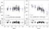 |
Fig. 4 Standard star calibration curve fit, derived with Eq. (1). The linear fit coefficients are displayed in the plots and listed in Table 3 together with the standard deviation of the residuals σ and the coefficient of determination r2. |
3. Statistical isochrone fitting
3.1. Method
To determined age, metallicity, distance modulus, and reddening in an objective and self-consistent way, we fit the CMD of each cluster against a set of synthetic CMDs using a numerical-statistical isochrone fitting. This method was extensively explained in previous works of our group, where it was applied to LMC clusters observed with HST/WFPC2 (Kerber et al. 2002, 2007; Kerber & Santiago 2005) and Galactic open clusters from 2MASS (Alves et al. 2012). In Paper I we analysed the CMDs of five SMC stellar clusters observed with SOAR/SOI using the same setup as in this paper. We therefore limit the description here and refer to the previous works for further details on the method.
The first step is to make a visual isochrone fitting to have a priori values for age, metallicity, distance and reddening. A grid of synthetic CMDs was constructed using the a priori information. All synthetic CMDs were simulated based on PARSEC isochrones (Bressan et al. 2012), assuming a binary fraction of 30%, a Salpeter IMF slope of α = 2.30, and photometric errors from the observations (Fig. 3). Figure 7 illustrates five synthetic CMDs for ages varying from 0.10 Gyr to 10 Gyr; the other parameters were kept fixed. They reproduce the observed features well, including the spread of points that is due to the photometric uncertainties and unresolved binaries.
The observed CMD was fitted against the grid of synthetic CMDs by applying the maximization of the likelihood statistics. The likelihood of each comparison was calculated as the product of the probabilities for the observed stars to be reproduced by each synthetic CMD – an implicit combination of age, metallicity, distance modulus, and reddening. The set of synthetic CMDs that maximize the likelihood were identified as the best, and their parameters were averaged out to obtain the final parameters and uncertainties for a given cluster. To avoid local maxima, we explored a wide range of values in the parameter space, considering virtually all solutions among the best ones. For further details we refer to the aforementioned works.
3.2. Results
We present the observed CMDs for the clusters and the respective synthetic CMD based on the best-fit parameters in Fig. 8. To present a cleaned CMD for each cluster, we statistically removed stars in accordance to their probability of being a non-cluster member (1−pmember) and the expected number of field stars within Rclus. The same isochrone is overplotted in the panels of observed and synthetic CMDs to guide the eye. For all nine clusters the similarity between synthetic and observed CMDs is reflected in the quality of the derived parameters shown in Table 5. We note that all CMDs present MSTO and RC, which is required to derive the parameters. The only exception is the young cluster Brück 6, where its well-defined main sequence constrains the fit. Kron 11 is the only cluster observed in the night with the poorer seeing, but still its CMD presents all features, in particular a clear MSTO and RC.
Stellar counts after the corrections for incompleteness and field contamination.
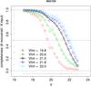 |
Fig. 5 Completeness curves for the reference cluster NGC 152. Different curves represent different annuli around the centre of the cluster in steps of 22″ (from 0′ to 1.8′). The curves in a crescent distance from the cluster centre are represented by red circles and a dotted line, green triangles and a dashed line, black diamonds and solid lines, blue inverted triangles and a dot-dashed line, and cyan squares and a long-dashed line. Uncertainty bars from the artificial star tests are presented in grey. The horizontal black dashed line at completeness level 0.5 marks the intersection with each line whose magnitudes are shown in the legend in each panel. |
The calibration cluster NGC 152 is 1.23 ± 0.07 Gyr old, with [Fe/H] = −0.87 ± 0.07 from our fitting procedure. Correnti et al. (in prep.) detected an extended main-sequence turnoff for this cluster assuming the same metallicity [Fe/H] = −0.6 and ages = 1.25, 1.4, and 1.6 Gyr. Our derived age agrees well with their findings, but our metallicity is more metal-poor. Rich et al. (2000) derived 1.3 < age < 2.0 Gyr assuming a metallicity of [Fe/H] = −0.7. From comparing our CMD to that of Rich et al., it is possible to see that their CMD is redder by 0.1−0.15 mag, which allows them to fit with a fainter turnoff by about 0.3−0.4 mag and hence to obtain an older age. Because of the possible problems with the magnitude system conversion by Rich et al. that we mentioned in Sect. 2.1 and also based on the compatibility of our ages with those from Correnti et al., we can say that all ages derived in this work and in Paper I are reliable. Neither Correnti et al. nor Rich et al. used a statistical fitting for the metallicities as we did to derive photometric abundances, therefore we can not use them as references. In Paper I, however, we compared our metallicity derivation for HW 40 with that derived using CaII triplet of individual stars by Parisi et al. (2015), and they were compatible. Therefore we can assume that our age and metallicity scales are satisfactory.
4. Age and metallicity gradients
Radial distributions of age and metallicity for the SMC seem to be tangled. With a significant dispersion, Parisi et al. (2014) have found an increasing trend on age distribution for a≲ 4.5° and decreasing above that. The opposite pattern is found for metallicity (Parisi et al. 2015), that is, values decrease until a< 4.5° and increase beyond this. In Paper I (Fig. 10) these trends were already detectable (see also Dobbie et al. 2014). Figure 10 shows age and [Fe/H] vs. distance from the SMC centre in terms of semi-major axis a. Parisi et al. (2015) explained the V shape by splitting their sample into two parts on a = 4° and averaging the metallicities in each bin in a. From this they found a very low gradient for clusters located at a< 4°, in agreement with other findings (e.g. Dobbie et al. 2014). However, they were unable to justify the behaviour of the metallicity distribution above a> 4°. We proposed a different explanation for the radial distribution in age and metallicity in Paper I and we endorse it here.
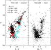 |
Fig. 6 V, (B−V) CMD for the reference cluster NGC 152 (R<Rclus, left panel) and the control field (R>Rrmfield, right panel). The point colours depend on the membership probability (pmember) for each star in the cluster direction. The horizontal dashed line corresponds to the magnitude limit, derived from the completeness curves around Rclus. |
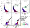 |
Fig. 7 Synthetic CMDs for different ages keeping other typical SMC parameters fixed as indicated in the plot. The colour scale indicates the logarithm of the number of stars to compose a Hess diagram used to fit the observer CMDs. |
Physical parameters determined in this work.
To discuss the gradients based on a large sample, we compiled ages and metallicities of SMC clusters available in the literature. We took weighted averages of the parameters, where the weights were attributed depending on the technique used, as follows. Ages from resolved photometry received weight 5, and those from integrated photometry or spectroscopy received weight 2. Metallicities derived using resolved spectroscopy received weight 5, those from resolved photometry received weight 3, and integrated spectroscopy received 2. This is not a complete catalogue from the literature, but it covers the most relevant works with large homogeneous samples: Dias et al. (2010), Parisi et al. (2015, 2009, 2014), Piatti et al. (2007a, 2008, 2011), Piatti (2011a, 2012a), Glatt et al. (2008b,a, 2010), Da Costa & Hatzidimitriou (1998), Mighell et al. (1998), Rafelski & Zaritsky (2005). Based on the catalogue of Bica et al. (2008), we selected 637 SMC clusters. We found ages for 346 of them and metallicities for 58 of them. The catalogue will be published separately.
The literature compilation of ages and metallicities for SMC clusters is representative for most of the cases. In Fig. 9 we show the cumulative distributions of distance to the centre a for each group of the SMC star cluster population. The reference curves in black were derived from the 637 clusters from the Bica et al. (2008) catalogue split into the four regions. The coloured curves represent ages and metallicities available for these clusters that are used in Fig. 10 and the following discussions. We ran Kolmogorov-Smirnov tests to check whether the samples are representative of their respective SMC component. For the main body, the age distribution is representative, but the metallicity distribution is missing for some clusters at around a ~ 1°. Wing and bridge clusters have a non-uniform distribution of ages, with more information available for inner clusters; the metallicity distribution is well covered. The counter-bridge and west halo samples are well spread over at all possible distances from the centre, and age and metallicity distributions represent this group well.
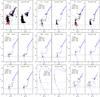 |
Fig. 8 Best isochrone fittings for all clusters. Left panels: cluster stars according to the membership probabilities (pmember). Right panels: synthetic CMD-generated parameters found for the best solution. The number of points is equal to the observed CMDs within the same magnitude limits. The horizontal dashed lines correspond to the magnitude limits used to compute the likelihood (brighter mag) and pmember (fainter mag). The solid blue line correspond to the PARSEC isochrones with the parameters found in Table 5. |
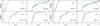 |
Fig. 9 Cumulative distributions of distance to the centre a for each group of the SMC star cluster population: main body, wing and bridge, counter-bridge, and west halo. Left panels show ages, right panels metallicities available in the literature compilation described in the text. Black curves are the distributions of all clusters, and the colour curves represent the clusters with available parameters. The numbers in the panels are the p-values obtained by applying the Kolmogorov-Smirnov test to the black and coloured curves. |
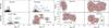 |
Fig. 10 Age and metallicity radial distributions in terms of the semi-major axis a in degrees, as done in Paper I. Age distributions are shown separately for the four components in the left panel, and the equivalent for metallicity is displayed in the right panel. Ages and metallicities are weighted averages from literature data as explained in the text. No results from this work are included here. Contours are the density maps considering a two-dimensional Gaussian around each point using their uncertainties. See text for details. |
In Fig. 10 we show the average age and metallicity for the clusters from the literature as described above, indicating the different regions in the galaxy: main body, wing and bridge, counter-bridge, and west halo following the definitions of Sect. 2.1. For each point we assumed an uncertainty in a of 0.2°, and uncertainties in age and metallicity from the literature. When uncertainties in metallicity were not available, we assumed 10% of [Fe/H]. These uncertainties were used to generate two-dimensional Gaussian distributions to populate the plots and trace the density curves shown in Fig. 10. The dispersion in the distributions may be caused in part by old and metal-poor clusters from the outskirts projected into the direction of the inner parts of the SMC. Moreover, the absolute value of the gradients can change if the distance scale a takes into account the three-dimensional shape of the SMC; the slope varies with sin(i), where i is the angle between the line of sight and the sky plane. However, if a gradient is detected in the projected distribution, it can be converted into the deprojected distribution if the angle i is known. The three-dimensional distribution is beyond the scope of this work and does not affect our conclusions here. Therefore we focus on the projected distributions below.
The SMC is classified as a dwarf irregular galaxy, which means that it is still forming stars. Glatt et al. (2010) showed that the bulk of recent star formation in the SMC occurs in its central bar and the older clusters are spread across the galaxy. If we assume that this was always the case for star formation in the SMC, we would expect age and metallicity gradients, with younger and metal-rich clusters in the innermost regions of the galaxy. In Fig. 10 cluster ages increase with a in the main body, although there is a large group of young clusters from Glatt et al. (2010). For metallicities the trend is cleaner and shows decreasing [Fe/H] with radial distance a. For the main body we confirm the findings from Glatt et al. We note that the discussions in Glatt et al. and in this work are based on the projected distribution of clusters.
For the wing and bridge, ages increase rapidly between 2°<a< 3° and there are sparse clusters beyond this distance that seem to have decreasing ages. Metallicities present larger uncertainties, nevertheless the distribution shows a valley at around a ≈ 4.5°. The combination of both distributions indicates that traces of the V-shape distribution described by Parisi et al. (2015) can be detected even in non-homogeneous average literature data. This deserves further investigation.
The counter-bridge has only a handful of clusters with available parameters, and it seems to be a tidal counterpart of the wing and bridge (Besla 2011; Diaz & Bekki 2012). Therefore its composition might be more complex. The age distribution seems to be increasing slowly with a but with a double trend. On the other hand, the metallicity distribution is monotonic, but with a large spread. More data are needed to confirm whether the distribution is double or not, and to confirm our first classification of counter-bridge clusters.
Finally, west halo clusters have monotonically increasing ages and monotonically decreasing metallicities until a< 6°. Beyond this lies only the peculiar cluster AM-3, which we discuss in Sect. 4.1.
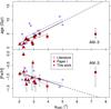 |
Fig. 11 Same as Fig. 10, but only with WH clusters. Blue diamonds are the same literature values as in the previous figure, excluding the clusters in common with our sample to avoid duplicates. Red squares are the results from Paper I for the WH, except AM-3. Red triangles are the results from this work. Blue lines are the linear fits to the literature points, red lines are the linear fits to our data points, and black lines are the linear fits to all points together. The parameters of these fits are presented in Table 6. |
To these distributions from literature, we now add our results for WH clusters in Fig. 11. Blue points are the same as those from Fig. 10, and red points represent the clusters analysed in Paper I and in this work. For duplicate clusters we removed the points from literature from the plot. Linear fits were made to the literature points (blue line), to our results (red line), and to both samples together (black line). The parameters from the fits are detailed in Table 6. The age gradient for WH clusters is found to be 2.6 ± 0.6 Gyr/°, with a coefficient of determination r2 = 0.5. For metallicity, the gradient is −0.19 ± 0.09 dex/° with r2 = 0.2. The coefficients r2 indicate that a linear fit is a good representation of the data distribution. The gradients are different from zero by more than 2σ. Therefore the radial gradients of age and metallicity for WH clusters are confirmed. Dobbie et al. (2014) derived a metallicity gradient of −0.075 ± 0.011 dex/° for field stars in the SMC for all stars internal to r< 5° from the centre. This region encompasses most of the star clusters, and we have demonstrated that it does not make sense to analyse the metallicity gradient of all clusters together. This explains why we derived a steeper gradient than that found by Dobbie et al.
Age and metallicity gradients for WH clusters.
Besla (2011) described the final distribution of gas and stars of the SMC after interaction with the LMC, following the scenario where the two galaxies are on their first close encounter with the Milky Way. In their Fig. 7.5 it becomes clear that stars in the external regions of the SMC present two large structures similar to spiral arms, one in the region of the wing and bridge, and the other starting in the region of the counter-bridge, which extends to the region of the WH. Although the aim of the simulations was to derive the general evolution of the Magellanic system and not to determine the exact final shape of the SMC, Fig. 12 shows that the distribution of the clusters qualitatively matches the star distributions from the simulation well. We note that the stars represented by the simulation in the figure are younger than 1 Gyr, but they represent the consequences of the tidal forces from the LMC-SMC interaction, which may have stripped the star clusters of all ages that were once in the main body. In this process, the gas movement could have formed some star clusters as well.
The WH is not part of the two arms, but corresponds to a fading stellar distribution outwards of the main body that appears to be a consequence of the tidal forces. The same is true for some counter-bridge clusters at the top of the plot in Fig. 12. This could indicate that the distribution of WH clusters is a sparse counterpart, a slice, of the main body in the outer region of the SMC that was stripped by the tidal force of the LMC. This is also indicated by the age and metallicity trends. The observations show that the trends of the main body and WH are similar, but the WH group is displaced by a = 2° (Fig. 10). More specifically, main-body clusters reach older ages of up to about 6 Gyr at a = 2°. WH clusters at this distance are younger with ages around 1 Gyr and increase with distance from the SMC centre. The metallicity of main-body clusters decreases to [Fe/H] ≈ −1.4 at a = 2° and WH clusters have [Fe/H] ≈ −0.8 decreasing with distance. We cannot rule out other scenarios to explain these breaks in age and metallicity trend between main body and west halo. Nevertheless, we were able to confirm and derive the gradients in the WH based on homogeneous results. In the model of Besla (2011) the interaction that originated the WH probably took place at about 100−160 Myr, which would agree with the strong common peaks in the cluster formation history of the clouds with OGLE (Pietrzynski & Udalski 2000). Brück 6, with 130 ± 40 Myr, appears to be a legacy of that enhancement, while the remaining clusters in Table 5 possibly show the results of tidal effects.
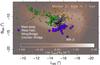 |
Fig. 12 Same as Fig. 1, but using Magellanic stream coordinates as defined by Nidever et al. (2008). Colours are the same as in Fig. 1, and the clusters are overplotted on a model by Besla (2011; adapted figure from Besla). |
Moreover, the very old and metal-poor clusters that were located in the outskirts of the main body before the interaction were sent to the outer region of the WH group. In particular, the most metal-poor globular cluster NGC 121 is located in this region. Its metallicity, previously obtained from low-resolution spectra and CMDs, estimated to be of [Fe/H] ~ −1.5 (Dias et al. 2010), was recently confirmed from analysis of spectra obtained with FLAMES at the VLT by Mucciarelli et al. (priv. comm.) as [Fe/H] ~ −1.4. This metallicity is compatible with the mean metallicity of field giants of [Fe/H] ~ −0.9/−1.0, as analysed by Mucciarelli (2014). We do not exclude the possibility of other scenarios to explain the gradients when splitting the clusters into the groups mentioned above. Dedicated models need to be discussed on the WH to address whether it is a tidal structure and to describe the processes involved.
Figure 13 shows the age-metallicity relation of SMC clusters with particular attention on the WH objects. We overplot the burst model of Pagel & Tautvaisiene (1998) and the major merger model of Tsujimoto & Bekki (2009) for reference. In the upper panel we show average parameters from the literature using colours and symbols to identify WH, main body, wing and bridge, and counter-bridge clusters, as in Fig. 10. In general, the clusters tend to follow the two chemical evolution models, but the dispersion in metallicity at a given age is as high as ~0.5 dex. When we select only WH objects (avoiding duplications as in Fig. 11), the clusters in the bottom panel show a lower dispersion in [Fe/H] for a given age around the model of Pagel & Tautvaisiene (1998). There are two exceptions: AM-3 and Kron 7. The first is probably not from the WH, but from the counter-bridge, as we discuss in the next section. The second has parameters derived mostly from integrated light, which are less accurate because of degeneracies. The only study based on six individual stars has been published by Da Costa & Hatzidimitriou (1998), who derived equivalent widths for CaII triplet lines. If we adopt the updated calibration of Saviane et al. (2012), the metallicity obtained for Kron 7 is [Fe/H] = −0.9 instead of the average ⟨ [Fe/H] ⟩ = −0.7 shown in the plot. This indicates that in fact WH clusters follow the burst model of Pagel & Tautvaisiene (1998) with a lower dispersion in metallicity. An alternative scenario would be the major merger 1−1 proposed by Tsujimoto & Bekki (2009) but 5 Gyr, not 7.5 Gyr ago. This would follow the argument of the model of Pagel & Tautvaisiene (1998) with a burst at about 4 Gyr ago.
A third interesting cluster is the most metal-rich and youngest of the sample, Brück 6, which was pointed out above as a possible product of the formation of the WH at the same epoch of the formation of the Magellanic bridge. Finally, we note that the dispersion in metallicity is not clearly explained by the radial distribution alone, since it mixes the external groups and the dispersion remains. Parisi et al. (2015) compared their data with five different chemical evolution models and also split the clusters in distance bins of a = 2°, and the dispersion remained. In summary, the age-metallicity relation appears to be different for different groups, as we also stated for age and metallicity gradients. More investigations on the other regions should therefore be carried out to solve this open question.
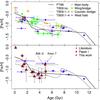 |
Fig. 13 Age-metallicity relation for SMC clusters. The upper panel shows the literature average, as in Fig. 10. The lower panel shows the WH clusters from the literature, Paper I, and this work. In both panels we overplot the burst chemical evolution model of Pagel & Tautvaisiene (1998) and the merger models of Tsujimoto & Bekki (2009), which correspond to no-merger and merger of progenitors with mass ratios of 1−1 and 1−4. |
4.1. AM-3: west halo or counter-bridge?
Based on Fig. 1, we classified AM-3 as a WH cluster because of its position in the sky plane. It is the outermost WH cluster at distance a = 7.3° from the SMC centre, while all other WH clusters are located within a< 5°. This cluster does not follow the gradients in age and metallicity, as shown in Fig. 10. Da Costa (1999) has pointed out that this cluster was the most distant from the SMC centre and still within the limits of the SMC field star and HI distribution. Recently, Besla (2011) and Diaz & Bekki (2012) have shown evidence for a stellar counterpart of the counter-bridge. In particular, Besla (2011) showed the predicted stellar distribution of the SMC after the tidal interaction with the LMC. We overplot the SMC clusters in the predicted stellar distribution and find a qualitatively good agreement of the main body, wing and bridge, counter-bridge, and west halo clusters. AM-3 is located in the tail of the counter-bridge structure predicted by the model (see Fig. 12). AM-3 age and metallicity seem to agree well with the extrapolation of the radial trends shown in Fig. 10. Moreover, AM-3 does not follow the general trend of the chemical evolution of the WH, as revealed by the age-metallicity relation in Fig. 13. Instead it seems to follow a trend together with counter-bridge clusters. Therefore it is possible that AM-3 is a counter-bridge cluster that was stripped to its current position following the counter-bridge arm described by the model.
5. Conclusions
We presented photometric parameters age, metallicity, distance, and reddening for nine clusters located in the WH of the SMC. Eight of them were studied for the first time, and NGC 152 was used as a reference cluster. We proposed to split the clusters in groups according to their position in the galaxy for a more enlightening analysis of the SMC history: main body, wing and bridge, counter-bridge, and WH. We focused on the last group. A detailed study of WH clusters has confirmed that to study the complex star formation and dynamical history of the SMC, it is crucial to analyse the galaxy region by region. The main results for the WH that led to this conclusion were as follows.
-
The age gradient of WH clusters is2.6 ± 0.6 Gyr/° with anegative linear coefficient equal to−3.7 ± 1.8 Gyr,indicating that the gradient is not compatible with the main bodyof the SMC. Moreover, in the transition from the main body to theWH at a = 2°, main-body clusters reach 6 Gyr, while WHhave ages around 1−2 Gyr, indicating adiscontinuity of radial gradients in cluster ages from the twogroups.
-
The metallicity gradient of WH clusters is more subtle than the age gradient, but the same comparisons are valid. The gradient is −0.19 ± 0.09 dex with a linear coefficient equal to −0.44 ± 0.27 dex, which is lower than the metallicities of the innermost clusters in the main body. In the boundary between main body and WH at a = 2°, main-body clusters extend to [Fe/H] ~−1.3, while WH clusters are around [Fe/H] ~−0.8, with an outlier with solar metallicity close to the main body, Brück 6, which might have formed during the tidal formation of the WH. There is no continuity in the metallicity gradient from the main body to the WH.
-
The age-metallicity relation of all SMC clusters presents a high dispersion in metallicity at a given age, but if only WH are plotted, the dispersion is significantly reduced and the distribution agrees with the burst chemical evolution model of Pagel & Tautvaisiene (1998).
-
The dynamical model from Besla et al. (2011) releases the stellar distribution in the SMC after tidal interactions with the LMC. Qualitatively, the cluster distribution agrees well with the predictions; this is very clear for main body, wing and bridge, and counter-bridge. WH clusters are located over a fading stellar distribution in the outer ranges of the main body between the two arms that represent the wing and bridge and counter-bridge.
-
The cluster AM-3 seems to be an important key to separating WH and counter-bridge because it is located in the region of the WH, but is far away, and it is also located in the tail of the extended arm shape of the counter-bridge. It follows the age and metallicity gradient and the age-metallicity relation of the counter-bridge, not of the WH.
-
The cluster Brück 6 seems to be an important witness of the recent epoch of interaction that created the Magellanic bridge about 100 Myr ago. During the possible tidal disruption that generated the west halo, Brück 6 would have been formed.
It is crucial to have homogeneous and precise ages and metallicities for SMC clusters in its four groups to understand the complexities in the history of our neighbour dwarf irregular galaxy. Spectroscopic metallicities and ages from CMDs from future observations are highly desired.
Acknowledgments
B.B., B.D., E.B. and L.K. acknowledge partial financial support from FAPESP, CNPq, CAPES, and the LACEGAL project, and the CAPES/CNPq for their financial support with the PROCAD project number 552236/2011-0. B.D. acknowledges ESO for the one-year studentship. S.O. acknowledges financial support of the University of Padova. B.D. acknowledges discussions and comments from G. Besla and C. Parisi. B.D. acknowledges T. Tsujimoto and G. Besla for kindly providing their models, and A. Mucciarelli for providing his preliminary results on NGC 121. L.K. acknowledges Matteo Correnti and Paul Goudfrooij for providing their CMD and results for NGC 152.
References
- Alves, V. M., Pavani, D. B., Kerber, L. O., & Bica, E. 2012, New Astron., 17, 488 [NASA ADS] [CrossRef] [Google Scholar]
- Besla, G. 2011, Ph.D. Thesis, Harvard University [Google Scholar]
- Besla, G., Kallivayalil, N., Hernquist, L., et al. 2007, ApJ, 668, 949 [NASA ADS] [CrossRef] [Google Scholar]
- Besla, G., Kallivayalil, N., Hernquist, L., et al. 2010, ApJ, 721, L97 [NASA ADS] [CrossRef] [Google Scholar]
- Bica, E., Bonatto, C., Dutra, C. M., & Santos, J. F. C. 2008, MNRAS, 389, 678 [NASA ADS] [CrossRef] [Google Scholar]
- Bressan, A., Marigo, P., Girardi, L., et al. 2012, MNRAS, 427, 127 [NASA ADS] [CrossRef] [Google Scholar]
- Caffau, E., Ludwig, H.-G., Steffen, M., Freytag, B., & Bonifacio, P. 2011, Sol. Phys., 268, 255 [NASA ADS] [CrossRef] [Google Scholar]
- Carrera, R., Gallart, C., Aparicio, A., et al. 2008, AJ, 136, 1039 [NASA ADS] [CrossRef] [Google Scholar]
- Chiosi, E., & Vallenari, A. 2007, A&A, 466, 165 [NASA ADS] [CrossRef] [EDP Sciences] [Google Scholar]
- Cignoni, M., Cole, A. A., Tosi, M., et al. 2013, ApJ, 775, 83 [NASA ADS] [CrossRef] [Google Scholar]
- Cioni, M.-R. L., Clementini, G., Girardi, L., et al. 2011, A&A, 527, A116 [NASA ADS] [CrossRef] [EDP Sciences] [Google Scholar]
- Crowl, H. H., Sarajedini, A., Piatti, A. E., et al. 2001, AJ, 122, 220 [NASA ADS] [CrossRef] [Google Scholar]
- Da Costa, G. S. 1999, in New Views of the Magellanic Clouds, eds. Y.-H. Chu, N. Suntzeff, J. Hesser, & D. Bohlender, IAU Symp., 190, 446 [Google Scholar]
- Da Costa, G. S., & Hatzidimitriou, D. 1998, AJ, 115, 1934 [NASA ADS] [CrossRef] [Google Scholar]
- Dias, B., Coelho, P., Barbuy, B., Kerber, L., & Idiart, T. 2010, A&A, 520, A85 [NASA ADS] [CrossRef] [EDP Sciences] [Google Scholar]
- Dias, B., Kerber, L. O., Barbuy, B., et al. 2014, A&A, 561, A106 [NASA ADS] [CrossRef] [EDP Sciences] [Google Scholar]
- Diaz, J. D., & Bekki, K. 2012, ApJ, 750, 36 [NASA ADS] [CrossRef] [Google Scholar]
- Dobbie, P. D., Cole, A. A., Subramaniam, A., & Keller, S. 2014, MNRAS, 442, 1680 [NASA ADS] [CrossRef] [Google Scholar]
- Gardiner, L. T., & Noguchi, M. 1996, MNRAS, 278, 191 [NASA ADS] [CrossRef] [Google Scholar]
- Girardi, L., Goudfrooij, P., Kalirai, J. S., et al. 2013, MNRAS, 431, 3501 [NASA ADS] [CrossRef] [Google Scholar]
- Glatt, K., Gallagher, III, J. S., Grebel, E. K., et al. 2008a, AJ, 135, 1106 [NASA ADS] [CrossRef] [Google Scholar]
- Glatt, K., Grebel, E. K., Sabbi, E., et al. 2008b, AJ, 136, 1703 [NASA ADS] [CrossRef] [Google Scholar]
- Glatt, K., Grebel, E. K., Gallagher, III, J. S., et al. 2009, AJ, 138, 1403 [NASA ADS] [CrossRef] [Google Scholar]
- Glatt, K., Grebel, E. K., & Koch, A. 2010, A&A, 517, A50 [NASA ADS] [CrossRef] [EDP Sciences] [Google Scholar]
- Harris, J., & Zaritsky, D. 2004, AJ, 127, 1531 [NASA ADS] [CrossRef] [Google Scholar]
- Harris, J., & Zaritsky, D. 2006, AJ, 131, 2514 [NASA ADS] [CrossRef] [Google Scholar]
- Kallivayalil, N., van der Marel, R. P., Besla, G., Anderson, J., & Alcock, C. 2013, ApJ, 764, 161 [NASA ADS] [CrossRef] [Google Scholar]
- Kerber, L. O., & Santiago, B. X. 2005, A&A, 435, 77 [NASA ADS] [CrossRef] [EDP Sciences] [Google Scholar]
- Kerber, L. O., Santiago, B. X., Castro, R., & Valls-Gabaud, D. 2002, A&A, 390, 121 [NASA ADS] [CrossRef] [EDP Sciences] [Google Scholar]
- Kerber, L. O., Santiago, B. X., & Brocato, E. 2007, A&A, 462, 139 [NASA ADS] [CrossRef] [EDP Sciences] [Google Scholar]
- Mathewson, D. S., Cleary, M. N., & Murray, J. D. 1974, ApJ, 190, 291 [NASA ADS] [CrossRef] [Google Scholar]
- Mighell, K. J., Sarajedini, A., & French, R. S. 1998, AJ, 116, 2395 [NASA ADS] [CrossRef] [Google Scholar]
- Moore, B., & Davis, M. 1994, MNRAS, 270, 209 [NASA ADS] [CrossRef] [Google Scholar]
- Mucciarelli, A. 2014, Astron. Nachr., 335, 79 [NASA ADS] [CrossRef] [Google Scholar]
- Nidever, D. L., Majewski, S. R., & Burton, W. B. 2008, ApJ, 679, 432 [NASA ADS] [CrossRef] [Google Scholar]
- Noël, N. E. D., Aparicio, A., Gallart, C., et al. 2009, ApJ, 705, 1260 [NASA ADS] [CrossRef] [Google Scholar]
- Pagel, B. E. J., & Tautvaisiene, G. 1998, MNRAS, 299, 535 [NASA ADS] [CrossRef] [Google Scholar]
- Parisi, M. C., Grocholski, A. J., Geisler, D., Sarajedini, A., & Clariá, J. J. 2009, AJ, 138, 517 [NASA ADS] [CrossRef] [Google Scholar]
- Parisi, M. C., Geisler, D., Carraro, G., et al. 2014, AJ, 147, 71 [NASA ADS] [CrossRef] [Google Scholar]
- Parisi, M. C., Geisler, D., Clariá, J. J., et al. 2015, AJ, 149, 154 [NASA ADS] [CrossRef] [Google Scholar]
- Piatti, A. E. 2011a, MNRAS, 416, L89 [NASA ADS] [CrossRef] [Google Scholar]
- Piatti, A. E. 2011b, MNRAS, 418, L69 [NASA ADS] [Google Scholar]
- Piatti, A. E. 2012a, ApJ, 756, L32 [NASA ADS] [CrossRef] [Google Scholar]
- Piatti, A. E. 2012b, MNRAS, 422, 1109 [NASA ADS] [CrossRef] [Google Scholar]
- Piatti, A. E. 2015, MNRAS, 451, 3219 [NASA ADS] [CrossRef] [Google Scholar]
- Piatti, A. E., Santos, Jr., J. F. C., Clariá, J. J., et al. 2005a, A&A, 440, 111 [NASA ADS] [CrossRef] [EDP Sciences] [Google Scholar]
- Piatti, A. E., Sarajedini, A., Geisler, D., Seguel, J., & Clark, D. 2005b, MNRAS, 358, 1215 [NASA ADS] [CrossRef] [Google Scholar]
- Piatti, A. E., Sarajedini, A., Geisler, D., Clark, D., & Seguel, J. 2007a, MNRAS, 377, 300 [NASA ADS] [CrossRef] [Google Scholar]
- Piatti, A. E., Sarajedini, A., Geisler, D., Gallart, C., & Wischnjewsky, M. 2007b, MNRAS, 381, L84 [NASA ADS] [Google Scholar]
- Piatti, A. E., Geisler, D., Sarajedini, A., Gallart, C., & Wischnjewsky, M. 2008, MNRAS, 389, 429 [NASA ADS] [CrossRef] [Google Scholar]
- Piatti, A. E., Clariá, J. J., Bica, E., et al. 2011, MNRAS, 417, 1559 [NASA ADS] [CrossRef] [Google Scholar]
- Pietrzynski, G., & Udalski, A. 2000, Acta Astron., 50, 337 [NASA ADS] [Google Scholar]
- Putman, M. E., Gibson, B. K., Staveley-Smith, L., et al. 1998, Nature, 394, 752 [NASA ADS] [CrossRef] [Google Scholar]
- Rafelski, M., & Zaritsky, D. 2005, AJ, 129, 2701 [NASA ADS] [CrossRef] [Google Scholar]
- Rich, R. M., Shara, M., Fall, S. M., & Zurek, D. 2000, AJ, 119, 197 [NASA ADS] [CrossRef] [Google Scholar]
- Rubele, S., Girardi, L., Kozhurina-Platais, V., Goudfrooij, P., & Kerber, L. 2011, MNRAS, 414, 2204 [NASA ADS] [CrossRef] [Google Scholar]
- Rubele, S., Girardi, L., Kerber, L., et al. 2015, MNRAS, 449, 639 [NASA ADS] [CrossRef] [Google Scholar]
- Saviane, I., da Costa, G. S., Held, E. V., et al. 2012, A&A, 540, A27 [NASA ADS] [CrossRef] [EDP Sciences] [Google Scholar]
- Searle, L., & Zinn, R. 1978, ApJ, 225, 357 [NASA ADS] [CrossRef] [Google Scholar]
- Shapley, H. 1940, Harvard College Observatory Bulletin, 914, 8 [Google Scholar]
- Sharpee, B., Stark, M., Pritzl, B., et al. 2002, AJ, 123, 3216 [NASA ADS] [CrossRef] [Google Scholar]
- Stanimirović, S., Staveley-Smith, L., & Jones, P. A. 2004, ApJ, 604, 176 [NASA ADS] [CrossRef] [Google Scholar]
- Stetson, P. B. 1987, PASP, 99, 191 [NASA ADS] [CrossRef] [Google Scholar]
- Subramanian, S., & Subramaniam, A. 2012, ApJ, 744, 128 [NASA ADS] [CrossRef] [Google Scholar]
- Tsujimoto, T., & Bekki, K. 2009, ApJ, 700, L69 [NASA ADS] [CrossRef] [Google Scholar]
- Vieira, K., Girard, T. M., van Altena, W. F., et al. 2010, AJ, 140, 1934 [NASA ADS] [CrossRef] [Google Scholar]
- Weisz, D. R., Dolphin, A. E., Skillman, E. D., et al. 2013, MNRAS, 431, 364 [NASA ADS] [CrossRef] [Google Scholar]
- Zaritsky, D., Harris, J., Thompson, I. B., Grebel, E. K., & Massey, P. 2002, AJ, 123, 855 [NASA ADS] [CrossRef] [Google Scholar]
Appendix A: Extra plots
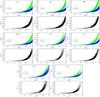 |
Fig. A.1 Same as Fig. 3 for all other clusters. |
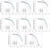 |
Fig. A.2 Same as Fig. 5 for all other clusters. Here different curves represent steps of 10″ (from 0′ to 0.8′) from the cluster centre. |
All Tables
West halo clusters with known parameters, selected as a subsample of Bica et al. (2008) using our definition.
All Figures
|
Fig. 1 Distribution of SMC star clusters as catalogued by Bica et al. (2008). Ellipses represent the distances from the SMC centre, as defined in Paper I. The different groups main body, wing and bridge, counter-bridge, and west halo are clearly identified as grey dots, green triangles, yellow squares, and blue diamonds. West halo clusters analysed in this work are highlighted with large red triangles, and those analysed in Paper I are displayed as large cyan circles. |
| In the text | |
|
Fig. 2 Sky maps of all nine clusters. All plots have the same contrast scale for magnitudes to allow a fair visual comparison. Blue circles indicate the adopted cluster size based on the catalogue of Bica et al. (2008) that were increased in some cases to include more stars for the statistical field-star decontamination. Red circles are the smallest limit around the cluster considered to select field stars, which has a radius of 2.5′ for NGC 152, and 1.5′ for the others. The values are provided in Table 4. |
| In the text | |
|
Fig. 3 Photometric errors from IRAF for the reference cluster NGC 152 in bands B and V, and colour B−V. |
| In the text | |
|
Fig. 4 Standard star calibration curve fit, derived with Eq. (1). The linear fit coefficients are displayed in the plots and listed in Table 3 together with the standard deviation of the residuals σ and the coefficient of determination r2. |
| In the text | |
|
Fig. 5 Completeness curves for the reference cluster NGC 152. Different curves represent different annuli around the centre of the cluster in steps of 22″ (from 0′ to 1.8′). The curves in a crescent distance from the cluster centre are represented by red circles and a dotted line, green triangles and a dashed line, black diamonds and solid lines, blue inverted triangles and a dot-dashed line, and cyan squares and a long-dashed line. Uncertainty bars from the artificial star tests are presented in grey. The horizontal black dashed line at completeness level 0.5 marks the intersection with each line whose magnitudes are shown in the legend in each panel. |
| In the text | |
|
Fig. 6 V, (B−V) CMD for the reference cluster NGC 152 (R<Rclus, left panel) and the control field (R>Rrmfield, right panel). The point colours depend on the membership probability (pmember) for each star in the cluster direction. The horizontal dashed line corresponds to the magnitude limit, derived from the completeness curves around Rclus. |
| In the text | |
|
Fig. 7 Synthetic CMDs for different ages keeping other typical SMC parameters fixed as indicated in the plot. The colour scale indicates the logarithm of the number of stars to compose a Hess diagram used to fit the observer CMDs. |
| In the text | |
|
Fig. 8 Best isochrone fittings for all clusters. Left panels: cluster stars according to the membership probabilities (pmember). Right panels: synthetic CMD-generated parameters found for the best solution. The number of points is equal to the observed CMDs within the same magnitude limits. The horizontal dashed lines correspond to the magnitude limits used to compute the likelihood (brighter mag) and pmember (fainter mag). The solid blue line correspond to the PARSEC isochrones with the parameters found in Table 5. |
| In the text | |
|
Fig. 9 Cumulative distributions of distance to the centre a for each group of the SMC star cluster population: main body, wing and bridge, counter-bridge, and west halo. Left panels show ages, right panels metallicities available in the literature compilation described in the text. Black curves are the distributions of all clusters, and the colour curves represent the clusters with available parameters. The numbers in the panels are the p-values obtained by applying the Kolmogorov-Smirnov test to the black and coloured curves. |
| In the text | |
|
Fig. 10 Age and metallicity radial distributions in terms of the semi-major axis a in degrees, as done in Paper I. Age distributions are shown separately for the four components in the left panel, and the equivalent for metallicity is displayed in the right panel. Ages and metallicities are weighted averages from literature data as explained in the text. No results from this work are included here. Contours are the density maps considering a two-dimensional Gaussian around each point using their uncertainties. See text for details. |
| In the text | |
|
Fig. 11 Same as Fig. 10, but only with WH clusters. Blue diamonds are the same literature values as in the previous figure, excluding the clusters in common with our sample to avoid duplicates. Red squares are the results from Paper I for the WH, except AM-3. Red triangles are the results from this work. Blue lines are the linear fits to the literature points, red lines are the linear fits to our data points, and black lines are the linear fits to all points together. The parameters of these fits are presented in Table 6. |
| In the text | |
|
Fig. 12 Same as Fig. 1, but using Magellanic stream coordinates as defined by Nidever et al. (2008). Colours are the same as in Fig. 1, and the clusters are overplotted on a model by Besla (2011; adapted figure from Besla). |
| In the text | |
|
Fig. 13 Age-metallicity relation for SMC clusters. The upper panel shows the literature average, as in Fig. 10. The lower panel shows the WH clusters from the literature, Paper I, and this work. In both panels we overplot the burst chemical evolution model of Pagel & Tautvaisiene (1998) and the merger models of Tsujimoto & Bekki (2009), which correspond to no-merger and merger of progenitors with mass ratios of 1−1 and 1−4. |
| In the text | |
|
Fig. A.1 Same as Fig. 3 for all other clusters. |
| In the text | |
|
Fig. A.2 Same as Fig. 5 for all other clusters. Here different curves represent steps of 10″ (from 0′ to 0.8′) from the cluster centre. |
| In the text | |
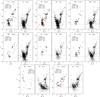 |
Fig. A.3 Same as Fig. 6 for all other clusters. |
| In the text | |
Current usage metrics show cumulative count of Article Views (full-text article views including HTML views, PDF and ePub downloads, according to the available data) and Abstracts Views on Vision4Press platform.
Data correspond to usage on the plateform after 2015. The current usage metrics is available 48-96 hours after online publication and is updated daily on week days.
Initial download of the metrics may take a while.