| Issue |
A&A
Volume 696, April 2025
|
|
|---|---|---|
| Article Number | A244 | |
| Number of page(s) | 15 | |
| Section | Galactic structure, stellar clusters and populations | |
| DOI | https://doi.org/10.1051/0004-6361/202452936 | |
| Published online | 29 April 2025 | |
Astrophysical properties of star clusters projected toward tidally perturbed SMC regions
1
Instituto Interdisciplinario de Ciencias Básicas (ICB), CONICET-UNCUYO,
Padre J. Contreras 1300,
M5502JMA,
Mendoza,
Argentina
2
Consejo Nacional de Investigaciones Científicas y Técnicas (CONICET),
Godoy Cruz 2290,
C1425FQB,
Buenos Aires,
Argentina
★ Corresponding author: This email address is being protected from spambots. You need JavaScript enabled to view it.
Received:
8
November
2024
Accepted:
11
March
2025
Abstract
We report on the astrophysical properties of a sample of star clusters in the Small Magellanic Cloud (SMC). We aimed to investigating the connection between the ages, heliocentric distances and metallicities of the selected star clusters with the existence of tidally perturbed or induced outermost SMC regions. We derived the star cluster fundamental parameters from relatively deep Survey of the Magellanic Stellar History (SMASH) color-magnitude diagrams (CMDs), cleaned from field star contamination, and compared them with a thousand synthetic CMDs covering a wide range of heliocentric distances, ages, and metal content. Heliocentric distances for 15 star clusters are derived for the first time, which represents an increase of ~50% of SMC clusters with estimated heliocentric distances. Analysis of the age-metallicity relationships (AMRs) of clusters located in the outermost regions distributed around the SMC and in the SMC Main Body reveals that they have followed the overall chemical enrichment history of the galaxy. However, since half of the studied clusters are situated in front of or behind the SMC Main Body, we concluded that they formed in the SMC and have traveled outward because of tidal effects from the interaction with the Large Magellanic Cloud (LMC). Furthermore, metal-rich clusters formed recently in some of these outermost regions from gas that was also dragged by tidal effects from the inner SMC. These findings lead to the SMC being considered as a galaxy scarred by the LMC tidal interaction with distance-perturbed and newly induced outermost stellar substructures.
Key words: methods: data analysis / techniques: photometric / Magellanic Clouds / galaxies: star clusters: general
© The Authors 2025
 Open Access article, published by EDP Sciences, under the terms of the Creative Commons Attribution License (https://creativecommons.org/licenses/by/4.0), which permits unrestricted use, distribution, and reproduction in any medium, provided the original work is properly cited.
This article is published in open access under the Subscribe to Open model. This email address is being protected from spambots. You need JavaScript enabled to view it. to support open access publication.
1 Introduction
The Magellanic Clouds are a pair of interacting irregular dwarf galaxies that are experiencing their first passages close to the Milky Way (Kallivayalil et al. 2013). In recent years, evidence of tidal effects on them has been observed. In the case of the Small Magellanic Cloud (SMC), several studies have attempted to precisely trace its internal kinematic behavior (Niederhofer et al. 2018; Zivick et al. 2018; Di Teodoro et al. 2019, and references therein). However, the magnitude of these tidal perturbations varies depending on the stellar population chosen and the observational data used (De Leo et al. 2020; Zivick et al. 2021; Niederhofer et al. 2021). Tidal effects have been found to be stronger in the outermost galaxy regions, particularly those facing the other interacting galaxy, while they are close to each other (Almeida et al. 2024; Cullinane et al. 2023). To date, SMC star clusters have not been extensively used as tracers of the internal kinematics of this galaxy (Maia et al. 2019; Piatti 2021). However, they offer several advantages for various reasons. For instance, their mean radial velocities and proper motions are derived from the average of several measurements of cluster members, which results in mean values based on sound statistics. Star clusters are also appropriate representatives of the internal motion of the SMC in comparison with the radial velocities and mean proper motions of stars aligned along different lines of sight through it. This remains valid even when it is derived from the separate analysis of different stellar populations of the galaxy field. Star clusters also have precisely determined ages and distances, so the internal kinematics of the SMC can be easily linked to the metallicities of the star clusters, and can thus provide an adequate framework for our understanding of both cluster formation and chemical and kinematic evolution of the galaxy.
Studying SMC star clusters distributed across the Southern Bridge, the SMC Wing, the West Halo, the Counter Bridge (Dias et al. 2014), among other tidally perturbed or induced SMC stellar substructures, provides insights into the origin of such stellar substructures, their dimensions and their location with respect to the SMC main body, their chemistry and their epoch of formation (see, e.g. Piatti 2022). We attempted to homogeneously estimate astrophysical properties (e.g., heliocentric distances, ages, and metallicities) of star clusters distributed in these selected SMC regions, aiming to perform an overall analysis of the magnitude of the tidal effects throughout the whole galaxy. We particularly focus, for the first time, on the estimation of star cluster heliocentric distances, which are remarkably lacking in the literature (Piatti 2023). For several decades, SMC star clusters were thought to be located at the mean galaxy distance, leading to misinterpretation of their formation history in the galaxy. Several studies have shown that the SMC is much more extended along the line of sight than its apparent size projected on the sky (Ripepi et al. 2017; Graczyk et al. 2020), which underscores the importance of deriving accurate heliocentric distances. This study is organized as follows: Section 2 describes the selection of the star cluster sample, alongside the data used in the analysis, the assignment of cluster star membership, and the estimation of the cluster astrophysical parameters, namely, reddening, age, distance, and metallicity. Section 3 details the resulting clusters’ properties, while in Sect. 4 we analyze the clusters with respect to the SMC stellar spatial distribution and star formation history. Section 5 summarizes the main conclusions of this work.
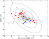 |
Fig. 1 Spatial distribution of Small Magellanic Cloud (SMC) clusters (Bica et al. 2020) represented with gray points. Red and blue filled circles represent the studied clusters with or without previous estimates of their heliocentric distances, respectively. The ellipses correspond to the framework devised by Piatti et al. (2007) for a= 2°, 4°, and 6°, respectively. |
2 Observational data
We selected 40 star clusters, mainly distributed across the outer SMC regions, using the catalog compiled by Bica et al. (2020). Table A.1 presents the most relevant fundamental parameters available in the literature, along with the methods employed to derive them. We used the framework devised by Piatti et al. (2007) as reference, which consists of concentric, equally aligned ellipses, with a position angle of 54° (measured anti-clockwise from the north) and a ratio of 2 between the semi-major and semi-minor axes. The selected star clusters are preferentially located outside the area covered by an ellipse with a semi-major axis of 2°. As mentioned in Sect. 1, they populate known perturbed or induced stellar substructures. Figure 1 illustrates the spatial distribution of the selected cluster sample. Fifteen clusters for which heliocentric distances have not been previously determined are highlighted with blue symbols.
Considering the overall low-brightness and compactness of the selected star clusters, the relatively deep photometric data provided by the Data Release 2 of the Survey of the Magellanic Stellar History (SMASH, Nidever et al. 2021) are suitable to perform a homogeneous estimation of their astrophysical parameters. The limiting magnitude extends beyond the 24th magnitude in the outskirts of the SMC, which is several magnitudes below the Main Sequence turnoff of a ~1 Gyr old cluster located at the distance of the SMC. The data of each selected cluster were retrieved from the Astro Data Lab1 interface, which is part of the Community Science and Data Center at NSF’s National Optical Infrared Astronomy Research Laboratory. We were particularly interested in the right ascension (RA) and declination (Dec) coordinates, the point spread function (PSF) g, i magnitudes and their respective errors, and the E(B − V) interstellar reddening and χ and SHARPNESS parameters of stellar sources located inside a circular region with a radius six times that of the cluster (Bica et al. 2020). We selected sources with 0.2 ≤ SHARPNESS ≤ 1.0 and χ < 0.5 with the aim of minimizing the contamination of bad pixels, cosmic rays, background galaxies, and unrecognized double stars.
To dis distinguish the main features of the observed cluster color-magnitude diagrams (CMDs), we first cleaned them from star field contamination using a statistical approach based on the procedure devised by Piatti & Bica (2012). This approach uses the magnitude and color of each star in the so-called reference star field CMD and finds the one closest in magnitude and color in the cluster’s CMD and subtracts it. We used the reddening corrected g0,i0 magnitudes computed from the observed g, i magnitudes, the E(B − V) values retrieved from SMASH, and the Aλ/E(B − V) ratios, for λ = g, i, given by Abott et al. (2018). In practice, we first selected stars located within the cluster circle with a radius equal to the cluster’s radius (Bica et al. 2020) and built the respective CMD. Secondly, we constructed 1000 CMDs with an area equal to the cluster circle and randomly located at a distance from the cluster center equal to 4.5 times the cluster’s radius. Thirdly, we subtracted stars from the cluster’s CMD with a similar distribution to those in the reference field CMDs. For this decontamination process, we applied one reference field CMD at a time. Therefore, we generated 1000 different cleaned cluster CMDs. Finally, we assigned membership probabilities based on the number of times a star survived the cleaning procedure. The probability is given by P = 1 − N/1000, where N represents the number of times a star was subtracted. Figure 2 illustrates the resulting membership probability distribution of stars in the field of HW56.
Using the field star decontaminated cluster photometry, we derived the clusters’ properties by employing routines of the Automated Stellar Cluster Analysis code (ASteCA, Perren et al. 2015). ASteCA enables the simultaneous derivation of the cluster’s metallicity, age, distance, and present day mass by generating a large number of synthetic CMDs and then selecting the one that best reproduces the cleaned star cluster CMD. The metallicity, age, distance, cluster present day mass and binary fraction derived from the generated synthetic CMD are adopted as the best-fitted cluster properties. To generate a statistically significant sample of synthetic CMDs, we adopted the initial mass function of Kroupa (2002) and a minimum mass ratio for the generation of binaries of 0.5. Cluster masses and binary fractions were set in the ranges 100–5000 M⊙ and 0.0–0.5, respectively. We also used PARSEC2 v1.2S isochrones (Bressan et al. 2012) for the SMASH photometric system, spanning metallicities Z from 0.0001 ([Fe/H] = −2.18 dex) up to 0.030 ([Fe/H] = 0.30 dex), in steps of ΔZ = 0.001, and log (age/yr) from 6.0 (1 Myr) up to 10.1 (12.5 Gyr) in steps of Δ(log(age/yr)) = 0.025. These metallicity and age ranges embrace the whole SMC age-metallicity relationship (Piatti & Geisler 2013).In some cases, we used smaller prior range values to ensure astrophysically meaningful results. We input the cluster SMASH photometry and the independently assigned membership probabilities for each observed star into ASteCA and derived the aforementioned cluster astrophysical parameters with their respective uncertainties. These errors were estimated from the standard bootstrap method described in Efron (1982). Table A.2 lists the resulting cluster parameters, Fig. 2 depicts the CMD of HW56 with the isochrone corresponding to the clusters’ parameters superimposed. Similar figures for the remaining cluster sample are included in the appendix.
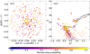 |
Fig. 2 Left: schematic finding chart of HW 56. The sizes of the symbols are proportional to the stars’ brightness. Right: cluster color-magnitude diagram with the theoretical isochrone (Bressan et al. 2012) corresponding to the adopted cluster parameters superimposed (see Table A.2). The color bar indicates the membership probability. |
3 Star cluster properties
Table A.2 shows that the selected cluster sample comprises SMC clusters spanning a wide age range (~3 Myr–7.06 Gyr), nearly any known SMC metallicity value ([Fe/H] ~ −1.3 dex to −0.25 dex), and a notable range of heliocentric distances (d ~ 36–75 kpc). Although a small number of clusters are known to have heliocentric distances that place them outside the Main Body of the SMC (~56–62 kpc, see Piatti 2022), we found nearly ten additional clusters located in the SMC periphery. Given the impact of these new heliocentric distances on our understanding of the formation and evolution of the SMC, we first validated our resulting astrophysical parameters by comparing them with those available in the literature (see Table A.1).
We conducted a thorough literature review to gather previous estimates of metallicity, age and heliocentric distance for the studied cluster sample. For clusters with more than one estimate, we averaged the published values, giving more weight to spectroscopic metallicities than those obtained from theoretical isochrone fitting to the clusters’ CMDs. When ages or heliocentric distances derived from CMD analyses were available, those from deeper and higher-quality photometry were assigned more weight. For completeness, we also included values of fundamental parameters found in the literature that we consider less accurate than our present values (B139, HW73). Table A.1 lists the adopted average values. We estimated accurate heliocentric distances, for the first time, for nearly 40% of the studied clusters. These results highlight the need for an observational campaign to perform a deep imaging survey to definitively address the 3D spatial distribution of the SMC cluster population. Such a survey would provide accurate heliocentric distances for a statistically significant sample of SMC clusters. At present, less than five% of the cataloged SMC star cluster population has individual heliocentric distance estimates (Piatti 2023). Until recently, photometric studies of SMC clusters assumed the SMC mean distance modulus. This assumption was valid in the context of less precise photometric data, which did not distinguish the distance variation of ~4.7 kpc (Δ (distance modulus) ~0.16 mag), corresponding to the full width at half maximum (FWHM) of the SMC Main Body (Graczyk et al. 2020).
Figures 3, 4 and 5 compare our derived true distance moduli, ages, and metallicities, respectively, with those found in the literature. We did not include B 139 and HW 73 in Fig. 3 because the available distance moduli are less accurate than our present estimates (this can be visually verified by comparing Fig. 2 of Piatti (2022) with the corresponding figures in the appendix. All three parameters show a very good agreement, with differences of Δ(log(age/yr)our − log(age/yr)lit. = 0.09 ± 0.07, Δ([Fe/H]our − [Fe/H]lit. = 0.073 ± 0.051 dex, and Δ((m − M)0our − (m − M)0lit.) = 0.14 ± 0.06 mag, respectively.
In the subsequent analysis, we focused on the most prominent star clusters in our sample without prior estimates of their heliocentric distances, with the aim of providing a detailed description of our resulting parameters.
For B99 we derived a mean true distance modulus of 17.9 mag, which in turn implied a mean heliocentric distance, d = 38.02 kpc. The mean age of the cluster and the metallicity were found to be 0.39 Gyr and [Fe/H] = −0.86, respectively. Our derived age is slightly higher than that obtained by Maia et al. (2014, 0.12 Gyr), while we found excellent agreement with the spectroscopic metallicity value derived by Parisi et al. (2015) ([Fe/H] = −0.84 dex).
The best-fitted theoretical isochrone for BS121 corresponds to an age of 2.63 Gyr and an overall metal content [Fe/H] = −0.78 dex, for a true distance modulus of 19.38 mag (d = 75.16 kpc). Both estimated cluster age and metallicity are in very good agreement with the values obtained by Parisi et al. (2009) and Parisi et al. (2015).
The CMD of H86-97 was satisfactorily reproduced by an isochrone of age = 0.19 Gyr and [Fe/H] = −0.73 dex, for a mean true distance modulus of 17.83 mag (d = 36.81 kpc). Our derived age is slightly younger than the age derived by Chiosi et al. (2006, 0.32 Gyr), while the present cluster metal content agrees well with the Ca II triplet metallicity obtained by Parisi et al. (2015).
The isochrone that best reproduces the CMD of OGLE-SMC 133 is that of an age of 2.14 Gyr, [Fe/H] = −0.88 dex, and true distance modulus of 18.54 mag (51.05 kpc). Although our derived metallicity is in agreement with that of Parisi et al. (2015) ([Fe/H] = −0.80 dex), our cluster age is slightly younger than the value obtained by Glatt et al. (2010, 6.29 Gyr).
The ages and metallicities of L7, L19, L58 and L116 are in very good agreement with the values retrieved from the literature (see Tables A.1 and A.2), while the derived mean true distance moduli are 18.76 mag (d = 56.49 kpc), 18.75 mag (d = 56.23 kpc), 18.64 mag (d = 53.46 kpc), and 18.13 mag (d = 42.27 kpc), respectively.
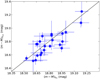 |
Fig. 3 Comparison between the derived distances moduli and those adopted from the literature. The solid line represents the identity relationship. |
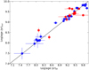 |
Fig. 4 Comparison between the derived ages and those adopted from the literature. Blue filled circles represent star clusters with previous estimates of their heliocentric distances, while red filled circles correspond to those without such estimates. The solid line represents the identity relation. |
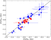 |
Fig. 5 Comparison between the derived metallicities and those adopted from the literature. Blue filled circles represent star clusters with previous estimates of their heliocentric distances, while red filled circles correspond to those without such estimates. The solid line represents the identity relation. |
4 Analysis and discussion
In the subsequent analysis we discuss the relationship between the clusters’ ages and metallicities with their positions in the SMC, in the context of the galaxy formation and its chemical and dynamical evolution. Our goal was to investigate whether star clusters projected toward tidally perturbed or induced SMC regions already formed there. From the confirmed cases, we assessed whether these regions are detachments of the old outer disk of the SMC or have been formed recently.
Figure 6 shows the variation of the derived metallicities with the cluster heliocentric distances. For clarity, we denoted the SMC Main Body boundaries with two vertical dashed lines. These values were derived from the best-fitted rotation disk of SMC star clusters obtained by Piatti (2021). A substantial proportion of the studied star cluster sample is located beyond these limits, predominantly at closer distances. The derived distances reveal a spatial distribution of SMC star clusters consistent with other independent studies that support the stripping scenario, caused by tidal interaction with the Large Magellanic Cloud (LMC; Subramanian et al. 2017; Cullinane et al. 2023; Nidever 2024). SMC outer disk star clusters have long been considered old, making them key to reconstructing the galaxy’s early formation and chemical enrichment history. In contrast, young star clusters are expected to be found in the inner galaxy region, where gas and dust still remain. From these perspectives, the presence of older, more metal-poor star clusters located in the outer SMC disk and younger, more metal-rich clusters in the inner galaxy, should not be surprising. However, the two closest star clusters to the Sun (H86-97 and B99) and two other clusters located behind the SMC Main Body (L95 and HW64) are young star clusters. This challenges our understanding of their roles in galaxy formation and evolution processes. Notably, both young star clusters located behind the SMC formed from a more chemically enriched material than their counterparts closer to the Sun. Nevertheless, for the majority of the studied star clusters, the younger clusters were more metal-rich, in agreement with the observed SMC cluster age-metallicity relationship (Piatti 2011).
Carpintero et al. (2013) modeled the dynamical interaction between the SMC and the LMC and their corresponding stellar cluster populations. Their simulations, probing a wide range of parameters for the orbits of both galaxies, showed that approximately 15% of the SMC clusters are captured by the LMC. Additionally 20–50% of its clusters are ejected into the intergalactic medium. These results enhance our understanding of the observed spatial distribution of the studied star clusters as objects potentially influenced by tidal interactions between both Magellanic Clouds. The LMC, being closer to the Sun than the SMC, may have stripped some SMC star clusters with heliocentric distances smaller than the mean SMC distance. Evidence of such an effect was found by Piatti & Lucchini (2022), who analyzed SMASH (Nidever et al. 2021) and Gaia EDR3 (Gaia Collaboration 2021) data of the recently discovered star cluster YMCA-1, concluding that it formed in the SMC and was subsequently stripped by the LMC. YMCA-1 is a 9.6 Gyr old, moderately metal-poor ([Fe/H] = −1.16 dex) star cluster located 60.9 kpc from the Sun, and ~17.1 kpc to the east of the LMC center.
Dias et al. (2014) and Dias et al. (2016) defined different zones throughout the outermost SMC regions: Northern Bridge, Counter Bridge, West Halo, Southern Bridge and Wing/Bridge, respectively (see Fig. 1 in Dias et al. 2022). For comparison, we superimposed these zones in Fig. 7. As shown, all of them contain star clusters analyzed in this work. In the figure we distinguished star clusters with or without previous heliocentric distance estimates using filled stars and circles, respectively. We used the heliocentric distances of the star clusters as indicators of the tidally perturbed or induced origin of the outermost SMC regions where they appear. For our analysis, we considered three different distance ranges: star clusters located closer than 55 kpc, between 55 kpc and 62 kpc, and beyond 62 kpc, according to Piatti (2021, see also our Fig. 6).
The Northern and Southern Bridges and the Wing/Bridge regions contain studied star clusters located in front of the SMC Main Body, supporting their tidal origin. These regions are facing the LMC, which is ~50 kpc from the Sun (de Grijs et al. 2014), suggesting the existence of a vast connecting region between both galaxies. This outcome is in very good agreement with the results obtained by Wagner-Kaiser & Sarajedini (2017), who derived metallicity and distance distributions of RR Lyrae variable stars to probe the structure of the Magellanic System as a whole, revealing a smooth transition that connects the galaxies. Star clusters closer than 55 kpc from the Sun are also seen toward the SMC Main Body, inside an ellipse of 2°. These star clusters confirm the larger extension of the galaxy along the line of sight, with a 3D shape of 1:2:4 along the declination, right ascension, and line of sight axes, respectively (Ripepi et al. 2017; Muraveva et al. 2018). Likewise, star clusters farther than 62 kpc from the Sun are observed in the Northern Bridge and projected toward the SMC Main Body.
In addition to the cluster heliocentric distances, their ages and metallicities also shed light on the origin of the SMC stellar structures to which the clusters belong. Comparison of the SMC age-metallicity relation (AMR) with those of its outermost regions contributes to understanding the extent of differential chemical evolution between these regions and the SMC.
For comparison, we used the AMR derived by Piatti & Geisler (2013) from Washington photometry of field stars distributed throughout the whole galaxy, and the theoretical values computed by Pagel & Tautvaisiene (1998) and Tsujimoto & Bekki (2009), respectively. Pagel & Tautvaisiene (1998) predicted an intensive star formation and chemical enrichment during the SMC formation epoch and a rapid burst of chemical enrichment about 3 Gyr ago. In comparison, Tsujimoto & Bekki (2009) predicted a major merger ~7.5 Gyr ago between two small galaxies of similar mass. Figure 8 depicts the resulting AMR for different outermost SMC regions, with star clusters colored according to their heliocentric distances.
In general, the studied clusters located in different SMC regions follow the overall SMC AMR. The most discordant star cluster appears to be L13, located in the West Halo (log(age/yr) = 8.97, [Fe/H] = −1.18 dex). Its relatively low metal content could suggest that it formed from poorly mixed gas. Star clusters located at heliocentric distances <55 kpc do not show distinct chemical differences from those populating the SMC Main Body. Based on these results, we propose that these clusters could have formed in the SMC and then migrated beyond the galaxy periphery, driven by tidal effects resulting from the interaction between the LMC and the SMC. In addition, the presence of relatively young and distant clusters (55 kpc > d > 62 kpc), located in the Northern Bridge, suggests that enriched gas has also reached the outermost regions of the SMC.
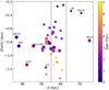 |
Fig. 6 Relationship between the derived metallicities and heliocentric distances of the studied star clusters, colored according to their derived ages. Filled stars and circles represent star clusters with or without previous estimates of their heliocentric distances, respectively. The vertical dashed lines delimit the extension of the SMC Main Body (Piatti 2023). |
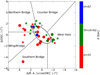 |
Fig. 7 Sky distribution of studied SMC star clusters. Symbol colors indicate the star cluster heliocentric distances. Dashed lines delineate the different outermost SMC regions (see text for details). Filled stars and circles represent star clusters with or without previous estimates of their heliocentric distances, respectively. |
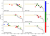 |
Fig. 8 Age-metallicity relationship for different SMC regions. Symbols are as detailed in Fig. 7. Superimposed are the observed age-metallicity relationship of Piatti & Geisler (2013) (black line), and the theoretical ones computed by Pagel & Tautvaisiene (1998) (blue line) and Tsujimoto & Bekki (2009) (orange lines). The dashed and solid orange lines correspond to cases without and with a merger of two similar mass galaxies, respectively. |
5 Conclusions
The SMC is known to have experienced tidal effects from its interaction with the LMC. As expected, its star cluster population bears evidence of this interaction history, which can be deciphered from the relationship between their ages, metallicities and distances. We selected 40 SMC star clusters with the aim of deriving their astrophysical properties and investigating the connection between the star clusters and the tidally perturbed or induced outermost SMC regions in which they are located. We used relatively deep cluster CMDs built from SMASH DR2 photometry and, after applying field star decontamination techniques, we derived fundamental parameters for each cluster.
We found homogeneously derived cluster ages, heliocentric distances and metallicities, which we have placed on a uniform scale, validated by reliable published estimates. The SMC is known to contain more than 650 star clusters (Bica et al. 2020). We have derived heliocentric distances for 15 star clusters for the first time, representing a ~50% increase in the number of SMC clusters with known distances (Piatti 2023). This small sample of clusters with derived heliocentric distances is distributed throughout the SMC Main Body, following a pattern similar to that of field stars. The presence of star clusters beyond the SMC body suggests the possibility that they could have been stripped due to interaction with the LMC.
Our analysis of the estimated cluster heliocentric distances revealed that nearly half of the studied star clusters are located beyond the SMC Main Body. Most of these clusters are located in front of the SMC, with some also located behind it. This result aligns with independent observational evidence of the tidal interaction between the LMC and the SMC. Our results confirm the existence of a physical connection between both galaxies, using star clusters are tracers.
From the analysis of the AMRs of star clusters located in different outermost SMC regions and in the Main Body of the galaxy, we found that intermediate-age and old star clusters generally follow the overall chemical enrichment history of the galaxy. Since some of these clusters are currently placed beyond the SMC Main Body boundaries, we conclude that they could have traveled outward due to the effects of the tidal interaction between the Magellanic Clouds. Moreover, not only star clusters formed in the SMC have migrated beyond its outskirts, chemically enriched gas has also migrated. This is supported by the formation of young, metal-rich star clusters in the Northern Bridge that also span a wide range of heliocentric distances. Therefore, the SMC has become a dwarf galaxy shaped by LMC tidal effects, with distance-perturbed and newly formed outermost stellar structures. Neglecting such a complex galaxy reality could lead to misinterpretation of the formation and evolution of the SMC, such as the present spatial distribution of the star cluster metallicities.
Acknowledgements
We thank the referee for the thorough reading of the manuscript and timely suggestions to improve it. This research uses services or data provided by the Astro Data Lab at NSF’s National Optical-Infrared Astronomy Research Laboratory. NSF’s OIR Lab is operated by the Association of Universities for Research in Astronomy (AURA), Inc. under a cooperative agreement with the National Science Foundation. Data for reproducing the figures and analysis in this work will be available upon request to the first author.
Appendix A Cleaned CMDs with the corresponding theoretical isochrones and tables with astrophysical parameters from the literature and those derived in our work for the selected clusters
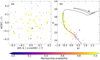 |
Fig. A.1 Schematic finding chart of Bruck 88 with the cluster’s color-magnitude diagram and the derived theoretical isochrone. |
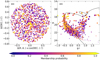 |
Fig. A.2 Schematic finding chart of Bruck 99 with the cluster’s color-magnitude diagram and the derived theoretical isochrone. |
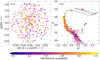 |
Fig. A.3 Schematic finding chart of Bruck 139 with the cluster’s color-magnitude diagram and the derived theoretical isochrone. |
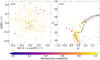 |
Fig. A.4 Schematic finding chart of Bruck 168 with the cluster’s color-magnitude diagram and the derived theoretical isochrone. |
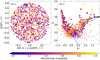 |
Fig. A.5 Schematic finding chart of BS121 with the cluster’s color-magnitude diagram and the derived theoretical isochrone. |
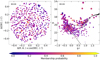 |
Fig. A.6 Schematic finding chart of BS188 with the cluster’s color-magnitude diagram and the derived theoretical isochrone. |
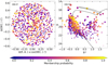 |
Fig. A.7 Schematic finding chart of H86-97 with the cluster’s color-magnitude diagram and the derived theoretical isochrone. |
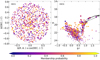 |
Fig. A.8 Schematic finding chart of HW31 with the cluster’s color-magnitude diagram and the derived theoretical isochrone. |
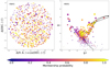 |
Fig. A.9 Schematic finding chart of HW41 with the cluster’s color-magnitude diagram and the derived theoretical isochrone. |
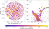 |
Fig. A.10 Schematic finding chart of HW47 with the cluster’s color-magnitude diagram and the derived theoretical isochrone. |
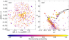 |
Fig. A.11 Schematic finding chart of HW67 with the cluster’s color-magnitude diagram and the derived theoretical isochrone. |
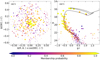 |
Fig. A.12 Schematic finding chart of HW73 with the cluster’s color-magnitude diagram and the derived theoretical isochrone. |
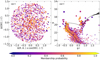 |
Fig. A.13 Schematic finding chart of HW77 with the cluster’s color-magnitude diagram and the derived theoretical isochrone. |
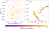 |
Fig. A.14 Schematic finding chart of HW84 with the cluster’s color-magnitude diagram and the derived theoretical isochrone. |
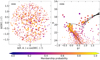 |
Fig. A.15 Schematic finding chart of HW86 with the cluster’s color-magnitude diagram and the derived theoretical isochrone. |
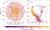 |
Fig. A.16 Schematic finding chart of IC1655 with the cluster’s color-magnitude diagram and the derived theoretical isochrone. |
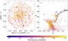 |
Fig. A.17 Schematic finding chart of L2 with the cluster’s color-magnitude diagram and the derived theoretical isochrone. |
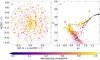 |
Fig. A.18 Schematic finding chart of L3 with the cluster’s color-magnitude diagram and the derived theoretical isochrone. |
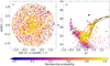 |
Fig. A.19 Schematic finding chart of L4 with the cluster’s color-magnitude diagram and the derived theoretical isochrone. |
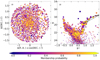 |
Fig. A.20 Schematic finding chart of L6 with the cluster’s color-magnitude diagram and the derived theoretical isochrone. |
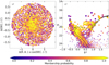 |
Fig. A.21 Schematic finding chart of L7 with the cluster’s color-magnitude diagram and the derived theoretical isochrone. |
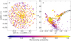 |
Fig. A.22 Schematic finding chart of L9 with the cluster’s color-magnitude diagram and the derived theoretical isochrone. |
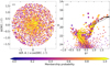 |
Fig. A.23 Schematic finding chart of L11 with the cluster’s color-magnitude diagram and the derived theoretical isochrone. |
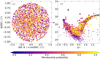 |
Fig. A.24 Schematic finding chart of L17 with the cluster’s color-magnitude diagram and the derived theoretical isochrone. |
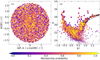 |
Fig. A.25 Schematic finding chart of L19 with the cluster’s color-magnitude diagram and the derived theoretical isochrone. |
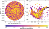 |
Fig. A.26 Schematic finding chart of L27 with the cluster’s color-magnitude diagram and the derived theoretical isochrone. |
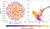 |
Fig. A.27 Schematic finding chart of L58 with the cluster’s color-magnitude diagram and the derived theoretical isochrone. |
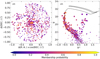 |
Fig. A.28 Schematic finding chart of L95 with the cluster’s color-magnitude diagram and the derived theoretical isochrone. |
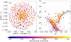 |
Fig. A.29 Schematic finding chart of L100 with the cluster’s color-magnitude diagram and the derived theoretical isochrone. |
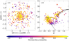 |
Fig. A.30 Schematic finding chart of L108 with the cluster’s color-magnitude diagram and the derived theoretical isochrone. |
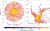 |
Fig. A.31 Schematic finding chart of L110 with the cluster’s color-magnitude diagram and the derived theoretical isochrone. |
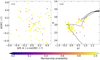 |
Fig. A.32 Schematic finding chart of L116 with the cluster’s color-magnitude diagram and the derived theoretical isochrone. |
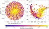 |
Fig. A.33 Schematic finding chart of NGC416 with the cluster’s color-magnitude diagram and the derived theoretical isochrone. |
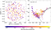 |
Fig. A.34 Schematic finding chart of OGLE 133 with the cluster’s color-magnitude diagram and the derived theoretical isochrone. |
Averaged literature values of fundamental parameters of the studied star clusters.
Derived fundamental parameters of the studied star clusters.
References
- Abott, T. M. C., Abdalla, F. B., Allam, S., et al. 2018, ApJS, 239, 18 [Google Scholar]
- Alcaino, G., Alvarado, F., Borissova, J., & Kurtev, R. 2003, A&A, 400, 917 [NASA ADS] [CrossRef] [EDP Sciences] [Google Scholar]
- Almeida, A., Majewski, S. R., Nidever, D. L., et al. 2024, MNRAS, 529, 3858 [Google Scholar]
- Bica, E., Westera, P., Kerber, L. d. O., et al. 2020, AJ, 159, 82 [Google Scholar]
- Bica, E., Westera, P., Kerber, L. d. O., et al. 2020, VizieR Online Data Catalog:J/AJ/ 159/82 [Google Scholar]
- Bressan, A., Marigo, P., Girardi, L., et al. 2012, MNRAS, 427, 127 [NASA ADS] [CrossRef] [Google Scholar]
- Brown, A. G. A., Vallenari, A., Prusti, T., et al. 2021, A&A, 649, A1 [NASA ADS] [CrossRef] [EDP Sciences] [Google Scholar]
- Carpintero, D. D., Gomez, F. A., & Piatti, A. E. 2013, MNRAS, 435, L63 [NASA ADS] [CrossRef] [Google Scholar]
- Chiosi, E., Vallenari, A., Held, E., Rizzi, L., & Moretti, A. 2006, A&A, 452, 179 [NASA ADS] [CrossRef] [EDP Sciences] [Google Scholar]
- Cullinane, L., Mackey, A., Da Costa, G., Koposov, S. E., & Erkal, D. 2023, MNRAS, 518, L25 [Google Scholar]
- De Grijs, R., & Bono, G. 2015, AJ, 149, 179 [CrossRef] [Google Scholar]
- de Grijs, R., Wicker, J. E., & Bono, G. 2014, AJ, 147, 122 [Google Scholar]
- De Bortoli, B. J., Parisi, M. C., Bassino, L. P., et al. 2022, A&A, 664, A168 [NASA ADS] [CrossRef] [EDP Sciences] [Google Scholar]
- De Leo, M., Carrera, R., Noël, N. E., et al. 2020, MNRAS, 495, 98 [Google Scholar]
- Di Teodoro, E. M., McClure-Griffiths, N., Jameson, K., et al. 2019, MNRAS, 483, 392 [Google Scholar]
- Dias, B., Angelo, M. S., Oliveira, R. A. P. d., et al. 2021, A&A, 647, L9 [NASA ADS] [CrossRef] [EDP Sciences] [Google Scholar]
- Dias, B., Kerber, L. d. O., Barbuy, B., et al. 2014, A&A, 561, A106 [NASA ADS] [CrossRef] [EDP Sciences] [Google Scholar]
- Dias, B., Kerber, L., Barbuy, B., Bica, E., & Ortolani, S. 2016, A&A, 591, A11 [NASA ADS] [CrossRef] [EDP Sciences] [Google Scholar]
- Dias, B., Parisi, M. C., Angelo, M., et al. 2022, MNRAS, 512, 4334 [NASA ADS] [CrossRef] [Google Scholar]
- Efron, B. 1982, The Jackknife, the Bootstrap and other Resampling Plans (SIAM) [CrossRef] [Google Scholar]
- Gaia Collaboration (Prusti, T., et al.) 2016, A&A, 595, A1 [NASA ADS] [CrossRef] [EDP Sciences] [Google Scholar]
- Gatto, M., Ripepi, V., Bellazzini, M., et al. 2021, MNRAS, 507, 3312 [NASA ADS] [CrossRef] [Google Scholar]
- Glatt, K., Grebel, E. K., Sabbi, E., et al. 2008, AJ, 136, 1703 [Google Scholar]
- Glatt, K., Grebel, E. K., & Koch, A. 2010, A&A, 517, A50 [CrossRef] [EDP Sciences] [Google Scholar]
- Graczyk, D., Pietrzyński, G., Thompson, I. B., et al. 2020, ApJ, 904, 13 [Google Scholar]
- Kallivayalil, N., Van der Marel, R. P., Besla, G., Anderson, J., & Alcock, C. 2013, ApJ, 764, 161 [NASA ADS] [CrossRef] [Google Scholar]
- Kroupa, P. 2002, Science, 295, 82 [Google Scholar]
- Livanou, E., Dapergolas, A., Kontizas, M., et al. 2013, A&A, 554, A16 [NASA ADS] [CrossRef] [EDP Sciences] [Google Scholar]
- Maia, F., Piatti, A. E., & Santos Jr, J. F. 2014, MNRAS, 437, 2005 [Google Scholar]
- Maia, F. F., Dias, B., Santos Jr, J. F., et al. 2019, MNRAS, 484, 5702 [Google Scholar]
- Milone, A. P., Cordoni, G., Marino, A., et al. 2023, A&A, 672, A161 [NASA ADS] [CrossRef] [EDP Sciences] [Google Scholar]
- Muraveva, T., Subramanian, S., Clementini, G., et al. 2018, MNRAS, 473, 3131 [Google Scholar]
- Narloch, W., Pietrzyński, G., Gieren, W., et al. 2021, A&A, 647, A135 [NASA ADS] [CrossRef] [EDP Sciences] [Google Scholar]
- Nayak, P., Subramaniam, A., Choudhury, S., & Sagar, R. 2018, A&A, 616, A187 [NASA ADS] [CrossRef] [EDP Sciences] [Google Scholar]
- Nidever, D. L. 2024, MNRAS, 533, 3238 [Google Scholar]
- Nidever, D. L., Olsen, K., Choi, Y., et al. 2021, AJ, 161, 74 [NASA ADS] [CrossRef] [Google Scholar]
- Niederhofer, F., Cioni, M.-R., Rubele, S., et al. 2018, A&A, 613, L8 [NASA ADS] [CrossRef] [EDP Sciences] [Google Scholar]
- Niederhofer, F., Cioni, M.-R. L., Rubele, S., et al. 2021, MNRAS, 502, 2859 [Google Scholar]
- Oliveira, R., Maia, F., Barbuy, B., et al. 2023, MNRAS, 524, 2244 [NASA ADS] [CrossRef] [Google Scholar]
- Pagel, B. E. J., & Tautvaisiene, G. 1998, MNRAS, 299, 535 [Google Scholar]
- Parisi, M., Grocholski, A., Geisler, D., Sarajedini, A., & Clariá, J. 2009, AJ, 138, 517 [NASA ADS] [CrossRef] [Google Scholar]
- Parisi, M. C., Geisler, D., Carraro, G., et al. 2014, AJ, 147, 71 [Google Scholar]
- Parisi, M. C., Geisler, D., Clariá, J. J., et al. 2015, AJ, 149, 154 [Google Scholar]
- Parisi, M. C., Gramajo, L. V., Geisler, D., et al. 2022, A&A, 662, A75 [NASA ADS] [CrossRef] [EDP Sciences] [Google Scholar]
- Perren, G. I., Vazquez, R. A., & Piatti, A. E. 2015, A&A, 576, A6 [NASA ADS] [CrossRef] [EDP Sciences] [Google Scholar]
- Piatti, A. E. 2011, MNRAS, 418, L69 [NASA ADS] [Google Scholar]
- Piatti, A. E. 2021, A&A, 650, A52 [NASA ADS] [CrossRef] [EDP Sciences] [Google Scholar]
- Piatti, A. E. 2022, MNRAS, 509, 3462 [Google Scholar]
- Piatti, A. E. 2023, MNRAS, 526, 391 [Google Scholar]
- Piatti, A. E., & Bica, E. 2012, MNRAS, 425, 3085 [Google Scholar]
- Piatti, A. E., & Geisler, D. 2013, AJ, 145, 17 [Google Scholar]
- Piatti, A. E., & Lucchini, S. 2022, MNRAS, 515, 4005 [Google Scholar]
- Piatti, A. E., Santos Jr, J. F., Clariá, J. J., et al. 2001, MNRAS, 325, 792 [NASA ADS] [CrossRef] [Google Scholar]
- Piatti, A. E., Sarajedini, A., Geisler, D., Seguel, J., & Clark, D. 2005, MNRAS, 358, 1215 [Google Scholar]
- Piatti, A. E., Sarajedini, A., Geisler, D., Gallart, C., & Wischnjewsky, M. 2007, MNRAS, 382, 1203 [Google Scholar]
- Piatti, A. E., Clariá, J. J., Bica, E., et al. 2011, MNRAS, 417, 1559 [NASA ADS] [CrossRef] [Google Scholar]
- Ripepi, V., Cioni, M.-R. L., Moretti, M. I., et al. 2017, MNRAS, 472, 808 [Google Scholar]
- Saroon, S., Dias, B., Tsujimoto, T., et al. 2023, A&A, 677, A35 [NASA ADS] [CrossRef] [EDP Sciences] [Google Scholar]
- Subramanian, S., Rubele, S., Sun, N.-C., et al. 2017, MNRAS, 467, 2980 [NASA ADS] [Google Scholar]
- Tsujimoto, T., & Bekki, K. 2009, ApJ, 700, L69 [Google Scholar]
- Wagner-Kaiser, R., & Sarajedini, A. 2017, MNRAS, 466, 4138 [Google Scholar]
- Zivick, P., Kallivayalil, N., van der Marel, R. P., et al. 2018, ApJ, 864, 55 [Google Scholar]
- Zivick, P., Kallivayalil, N., & van der Marel, R. P. 2021, ApJ, 910, 36 [Google Scholar]
All Tables
Averaged literature values of fundamental parameters of the studied star clusters.
All Figures
|
Fig. 1 Spatial distribution of Small Magellanic Cloud (SMC) clusters (Bica et al. 2020) represented with gray points. Red and blue filled circles represent the studied clusters with or without previous estimates of their heliocentric distances, respectively. The ellipses correspond to the framework devised by Piatti et al. (2007) for a= 2°, 4°, and 6°, respectively. |
| In the text | |
|
Fig. 2 Left: schematic finding chart of HW 56. The sizes of the symbols are proportional to the stars’ brightness. Right: cluster color-magnitude diagram with the theoretical isochrone (Bressan et al. 2012) corresponding to the adopted cluster parameters superimposed (see Table A.2). The color bar indicates the membership probability. |
| In the text | |
|
Fig. 3 Comparison between the derived distances moduli and those adopted from the literature. The solid line represents the identity relationship. |
| In the text | |
|
Fig. 4 Comparison between the derived ages and those adopted from the literature. Blue filled circles represent star clusters with previous estimates of their heliocentric distances, while red filled circles correspond to those without such estimates. The solid line represents the identity relation. |
| In the text | |
|
Fig. 5 Comparison between the derived metallicities and those adopted from the literature. Blue filled circles represent star clusters with previous estimates of their heliocentric distances, while red filled circles correspond to those without such estimates. The solid line represents the identity relation. |
| In the text | |
|
Fig. 6 Relationship between the derived metallicities and heliocentric distances of the studied star clusters, colored according to their derived ages. Filled stars and circles represent star clusters with or without previous estimates of their heliocentric distances, respectively. The vertical dashed lines delimit the extension of the SMC Main Body (Piatti 2023). |
| In the text | |
|
Fig. 7 Sky distribution of studied SMC star clusters. Symbol colors indicate the star cluster heliocentric distances. Dashed lines delineate the different outermost SMC regions (see text for details). Filled stars and circles represent star clusters with or without previous estimates of their heliocentric distances, respectively. |
| In the text | |
|
Fig. 8 Age-metallicity relationship for different SMC regions. Symbols are as detailed in Fig. 7. Superimposed are the observed age-metallicity relationship of Piatti & Geisler (2013) (black line), and the theoretical ones computed by Pagel & Tautvaisiene (1998) (blue line) and Tsujimoto & Bekki (2009) (orange lines). The dashed and solid orange lines correspond to cases without and with a merger of two similar mass galaxies, respectively. |
| In the text | |
|
Fig. A.1 Schematic finding chart of Bruck 88 with the cluster’s color-magnitude diagram and the derived theoretical isochrone. |
| In the text | |
|
Fig. A.2 Schematic finding chart of Bruck 99 with the cluster’s color-magnitude diagram and the derived theoretical isochrone. |
| In the text | |
|
Fig. A.3 Schematic finding chart of Bruck 139 with the cluster’s color-magnitude diagram and the derived theoretical isochrone. |
| In the text | |
|
Fig. A.4 Schematic finding chart of Bruck 168 with the cluster’s color-magnitude diagram and the derived theoretical isochrone. |
| In the text | |
|
Fig. A.5 Schematic finding chart of BS121 with the cluster’s color-magnitude diagram and the derived theoretical isochrone. |
| In the text | |
|
Fig. A.6 Schematic finding chart of BS188 with the cluster’s color-magnitude diagram and the derived theoretical isochrone. |
| In the text | |
|
Fig. A.7 Schematic finding chart of H86-97 with the cluster’s color-magnitude diagram and the derived theoretical isochrone. |
| In the text | |
|
Fig. A.8 Schematic finding chart of HW31 with the cluster’s color-magnitude diagram and the derived theoretical isochrone. |
| In the text | |
|
Fig. A.9 Schematic finding chart of HW41 with the cluster’s color-magnitude diagram and the derived theoretical isochrone. |
| In the text | |
|
Fig. A.10 Schematic finding chart of HW47 with the cluster’s color-magnitude diagram and the derived theoretical isochrone. |
| In the text | |
|
Fig. A.11 Schematic finding chart of HW67 with the cluster’s color-magnitude diagram and the derived theoretical isochrone. |
| In the text | |
|
Fig. A.12 Schematic finding chart of HW73 with the cluster’s color-magnitude diagram and the derived theoretical isochrone. |
| In the text | |
|
Fig. A.13 Schematic finding chart of HW77 with the cluster’s color-magnitude diagram and the derived theoretical isochrone. |
| In the text | |
|
Fig. A.14 Schematic finding chart of HW84 with the cluster’s color-magnitude diagram and the derived theoretical isochrone. |
| In the text | |
|
Fig. A.15 Schematic finding chart of HW86 with the cluster’s color-magnitude diagram and the derived theoretical isochrone. |
| In the text | |
|
Fig. A.16 Schematic finding chart of IC1655 with the cluster’s color-magnitude diagram and the derived theoretical isochrone. |
| In the text | |
|
Fig. A.17 Schematic finding chart of L2 with the cluster’s color-magnitude diagram and the derived theoretical isochrone. |
| In the text | |
|
Fig. A.18 Schematic finding chart of L3 with the cluster’s color-magnitude diagram and the derived theoretical isochrone. |
| In the text | |
|
Fig. A.19 Schematic finding chart of L4 with the cluster’s color-magnitude diagram and the derived theoretical isochrone. |
| In the text | |
|
Fig. A.20 Schematic finding chart of L6 with the cluster’s color-magnitude diagram and the derived theoretical isochrone. |
| In the text | |
|
Fig. A.21 Schematic finding chart of L7 with the cluster’s color-magnitude diagram and the derived theoretical isochrone. |
| In the text | |
|
Fig. A.22 Schematic finding chart of L9 with the cluster’s color-magnitude diagram and the derived theoretical isochrone. |
| In the text | |
|
Fig. A.23 Schematic finding chart of L11 with the cluster’s color-magnitude diagram and the derived theoretical isochrone. |
| In the text | |
|
Fig. A.24 Schematic finding chart of L17 with the cluster’s color-magnitude diagram and the derived theoretical isochrone. |
| In the text | |
|
Fig. A.25 Schematic finding chart of L19 with the cluster’s color-magnitude diagram and the derived theoretical isochrone. |
| In the text | |
|
Fig. A.26 Schematic finding chart of L27 with the cluster’s color-magnitude diagram and the derived theoretical isochrone. |
| In the text | |
|
Fig. A.27 Schematic finding chart of L58 with the cluster’s color-magnitude diagram and the derived theoretical isochrone. |
| In the text | |
|
Fig. A.28 Schematic finding chart of L95 with the cluster’s color-magnitude diagram and the derived theoretical isochrone. |
| In the text | |
|
Fig. A.29 Schematic finding chart of L100 with the cluster’s color-magnitude diagram and the derived theoretical isochrone. |
| In the text | |
|
Fig. A.30 Schematic finding chart of L108 with the cluster’s color-magnitude diagram and the derived theoretical isochrone. |
| In the text | |
|
Fig. A.31 Schematic finding chart of L110 with the cluster’s color-magnitude diagram and the derived theoretical isochrone. |
| In the text | |
|
Fig. A.32 Schematic finding chart of L116 with the cluster’s color-magnitude diagram and the derived theoretical isochrone. |
| In the text | |
|
Fig. A.33 Schematic finding chart of NGC416 with the cluster’s color-magnitude diagram and the derived theoretical isochrone. |
| In the text | |
|
Fig. A.34 Schematic finding chart of OGLE 133 with the cluster’s color-magnitude diagram and the derived theoretical isochrone. |
| In the text | |
Current usage metrics show cumulative count of Article Views (full-text article views including HTML views, PDF and ePub downloads, according to the available data) and Abstracts Views on Vision4Press platform.
Data correspond to usage on the plateform after 2015. The current usage metrics is available 48-96 hours after online publication and is updated daily on week days.
Initial download of the metrics may take a while.