| Issue |
A&A
Volume 695, March 2025
|
|
|---|---|---|
| Article Number | L9 | |
| Number of page(s) | 8 | |
| Section | Letters to the Editor | |
| DOI | https://doi.org/10.1051/0004-6361/202453506 | |
| Published online | 10 March 2025 | |
Letter to the Editor
The VISCACHA Survey
XII. SL 2: Age gap cluster in the southwestern Large Magellanic Cloud
1
Departamento de Física, Instituto de Ciências Exatas, Universidade Federal de Minas Gerais (UFMG), Av. Antônio Carlos 6627, Belo Horizonte 31270-901, Brazil
2
Departamento de Ciencias Físicas, Instituto de Astrofísica, Facultad de Ciencias Exactas, Universidad Andres Bello (UNAB), Av. Fernandez Concha 700, 7591538 Las Condes, Santiago, Chile
3
Instituto de Física, Universidade Federal do Rio de Janeiro (UFRJ), Av. Athos da Silveira Ramos, 149, Rio de Janeiro 21941-909, Brazil
4
Departamento de Astronomia, Universidade Federal do Rio Grande do Sul (UFRGS), Av. Osvaldo Aranha, s/n, Porto Alegre 91501-970, Brazil
5
Departamento de Ciências Exatas, Universidade Estadual de Santa Cruz (UESC), Rod.Jorge Amado km 16, 45662-900 Ilhéus, Brazil
6
Departamento de Estatística, Física e Matemática, Universidade Federal de São João del-Rei, Campus Alto Paraopeba, Rod. MG 443, km 7, Ouro Branco 36420-000, Brazil
7
Rubin Observatory Project Office, 950 N. Cherry Ave., Tucson, AZ 85719, USA
8
Astronomical Observatory, University of Warsaw, Al. Ujazdowskie 4, 00-478 Warszawa, Poland
9
Max Planck Institute for Astronomy, Königstuhl 17, D-69117 Heidelberg, Germany
10
Instituto de Astronomía, Universidad Católica del Norte, Av. Angamos 0610, Antofagasta, Chile
⋆ Corresponding author; This email address is being protected from spambots. You need JavaScript enabled to view it.
Received:
18
December
2024
Accepted:
25
February
2025
Abstract
Context. In the Large Magellanic Cloud (LMC), only seven star clusters have been discovered to be older than ∼4 Gyr and younger than ∼10 Gyr, placing them in what is known as the age gap.
Aims. We aim to analyze the photometric data from the VISCACHA survey in the V and I bands to determine, for the first time, the astrophysical parameters of SL 2, revealing that the cluster is indeed situated within the age gap.
Methods. We used our newly developed SIESTA code to carry out a statistical isochrone fitting with synthetic color-magnitude diagrams (CMDs) to determine the cluster age, metallicity, distance, color excess, and binary fraction with two grids of stellar evolution models. In addition, the cluster mass was estimated based on its integrated magnitude.
Results. The ages obtained from isochrone fitting are compatible with the age gap, amounting to (7.17 ± 0.35) Gyr when using PARSEC-COLIBRI isochrones and (8.02 ± 0.45) Gyr when using MIST. Notably, SL 2 is the first age gap cluster discovered in the southern region of the LMC. The mass of the cluster is considerably smaller than that of the group of older LMC clusters.
Conclusions. SL 2 has a comparable metallicity to the other two age gap clusters with similar ages, namely, ESO 121-03 and KMHK 1592, as well as the LMC field star population. While the discovery of a new cluster with such characteristics could be seen as evidence that age gap clusters were formed in situ, the heliocentric distance of SL2 locates it far from the LMC center, akin to the SMC distance. Therefore, the question of its origin, alongside that of other age gap clusters, remains unresolved and open to further investigation.
Key words: Hertzsprung-Russell and C-M diagrams / Magellanic Clouds / galaxies: star clusters: individual: SL 2
© The Authors 2025
 Open Access article, published by EDP Sciences, under the terms of the Creative Commons Attribution License (https://creativecommons.org/licenses/by/4.0), which permits unrestricted use, distribution, and reproduction in any medium, provided the original work is properly cited.
This article is published in open access under the Subscribe to Open model. This email address is being protected from spambots. You need JavaScript enabled to view it. to support open access publication.
1. Introduction
One of the distinct features of the Large Magellanic Cloud (LMC) is that its star clusters are generally divided into two groups: one younger than ∼ 4 Gyr, with metallicities [Fe/H] ≈ −0.5 and another older than ∼ 12 Gyr with metallicities [Fe/H] ≈ −1.5 (see, e.g., Kerber et al. 2007; Narloch et al. 2022). Separating them is an interval of approximately 8 Gyr commonly referred to as the LMC “age gap” (Jensen et al. 1988; Olszewski et al. 1991), whereby very few clusters are observed.
Considering the physical origin of the age gap, Bekki et al. (2004), Bekki & Chiba (2005) proposed a model in which the LMC was formed distantly from the Milky Way (MW) and initially experienced a brief period of star formation, which formed the old, massive clusters, only to fall in a long quiescent period that ended around 3 Gyr ago, when the LMC approached the Small Magellanic Cloud (SMC). The ensuing tidal interactions triggered gas cloud collisions in the LMC, reigniting star formation.
This would explain the lack of star clusters in the aforementioned age gap. Studies of the LMC star formation history back up this scenario, by confirming that the star formation rate in the galaxy decreased in the same period as the age gap (Carrera et al. 2008; Harris & Zaritsky 2009; Piatti & Geisler 2013). Comparative studies with the star formation history in the SMC also suggest that the interaction between these two galaxies is a possible component of the resumption of star formation (Weisz et al. 2013; Massana et al. 2022). Even so, the same studies found a non-negligible number of field stars in this age range, which are expected to have been formed in clusters that later went through dissolution (Lada & Lada 2003; Baumgardt et al. 2013).
Understanding the age gap is essential for comprehending the star formation history and chemical evolution of the LMC, which ties into how this galaxy evolved and interacted with the MW and the SMC. Therefore, significant effort has been made to identify clusters in this age range (e.g., Balbinot et al. 2010; Gatto et al. 2020; Piatti 2021). Still, out of the more than 3100 catalogued clusters in the LMC (Bica et al. 2008), only seven have been found to be in the gap so far.
Initially, the younger limit of the gap was thought to be at ∼ 2.5 Gyr, however, the discovery of several clusters outside this interval prompted a revision, shifting the limit to 4 Gyr (Sarajedini 1998; Rich et al. 2001; Piatti et al. 2002). More recently, Pieres et al. (2016), using data from the Dark Energy Survey (DES; The Dark Energy Survey Collaboration 2005), identified NGC 1997 and DES001SC04 (discovered in the same paper) as clusters with ages between 4 and 4.5 Gyr. Gatto et al. (2022) characterized the cluster KMHK 1762 using data from the YMCA Survey (Gatto et al. 2024), obtaining an age of around 5.5 Gyr. In follow-up work, Gatto et al. (2024) discovered two new cluster candidates with ages 5.5 and 6.5 Gyr, leading to the authors’ suggestion that the young limit of the age gap might be even older, closer to 6 Gyr.
Amongst “genuine” age gap clusters, with ages between 6.5 and 10 Gyr, for many decades, ESO 121-03 was the only confirmed object. The cluster was first characterized by Mateo et al. (1986), who obtained two possible ages: (8 ± 2) Gyr or (10 ± 2) Gyr. Later, Mackey et al. (2006) used data from the Hubble Space Telescope (HST) to better constrain the age of this cluster between 8.3 and 9.8 Gyr. More recently, Milone et al. (2023) reanalyzed the same data, obtaining a younger age, of 6.9 Gyr, which is still consistent with the gap. A new cluster in this age range would only be found 36 years later by Piatti (2022) using images from the Gemini South telescope, which allowed them to identify KMHK 1592 as having an age of (8.0 ± 0.5) Gyr.
In this work, we present the identification of the star cluster SL 2 (also known as LW2 or KMHK2; firstly cataloged by Shapley & Lindsay 1963; Lynga & Westerlund 1963) as another genuine age-gap cluster. SL 2 is the first cluster in the age gap discovered in the southern region of the LMC. This determination was made possible using data from the VISCACHA (VIsible Soar photometry of star Clusters in tApii and Coxi HuguA) survey (Maia et al. 2019; Dias et al. 2020, with the first one referred to as Paper I), which is sufficiently deep (reaching V ≈ 23.5) to reach the cluster’s main sequence turn-off (MSTO), allowing for a reliable age determination.
2. Data and methodology
The photometric data for SL 2 were obtained by the VISCACHA Survey in the V, I bands using the ground layer, adaptive optics imager SAMI installed at the 4.1 m SOAR telescope (Tokovinin et al. 2016), reaching image quality of 0.75″ in the V band and 0.7″ in the I band. Table A.1 presents the log of the observations. Long exposures were performed reaching a photometric limit of V = 23.5, whereas short exposures were obtained to avoid saturation of the brightest stars. Data reduction, astrometric calibration, and photometry were performed following the procedure described in Paper I.
We evaluated the cluster size by fitting a three-parameter King (1962) function to its radial density profile (RDP):
 (1)
(1)
where σ represents the background subtracted stellar density at an angular distance, r, to the cluster center, while rc and rt are the core and tidal radii, respectively. The latter was determined to be (85 ± 5)″ and serves as the cluster truncation radius, effectively determining its size. The RDP, which is shown in Fig. A.1, was produced by evaluating the stellar density at concentric rings following of Paper I.
While the RDP is well-fit by the King’s profile beyond the cluster core, the fitted profile underpredicts the central density, in accord with simulations of clusters close to pre-core-collapse (Chatterjee et al. 2013; Zocchi et al. 2016). In the future, the structure of SL 2 can be evaluated in more detail by including a completeness correction to better evaluate the properties of its inner region (e.g., Gardin et al. 2024).
Before analyzing the cluster’s color-magnitude diagram (CMD), we performed a photometric decontamination to remove the contribution from field stars, using the method described in Maia et al. (2010). The process is summarized in Appendix B.
To determine the astrophysical parameters of the cluster, we used the SIESTA code1 (Ferreira et al. 2024). The code functions by comparing the Hess diagram of a given cluster, with the corresponding diagrams from synthetic populations, produced from a set of isochrones. Synthetic populations simulate the observed luminosity function, non-resolved binaries, and photometric uncertainties. The comparison between synthetic and observed data is performed using Markov chain Monte Carlo (MCMC) in a Bayesian approach. This allows us to determine the cluster’s age, metallicity, distance, color excess, and binary fraction.
One of the benefits of using a Bayesian approach is that prior distributions can be defined to enforce some previous knowledge regarding the cluster parameters. Uniform (uninformative), box priors were adopted in age constraining the parameter space between the limits of the isochrone grid. The same was done for the metallicity, since (to our knowledge) no spectroscopic information is available for SL 2 in the literature. For distances, another uniform, box prior was used, between 35 and 65 kpc. For color excess, we used a Gaussian prior based on the value of E(B − V) = 0.11 obtained from the extinction maps of Schlegel et al. (1998), with a standard deviation of 16% (σE(B − V) = 0.02), which is the accuracy estimated by the authors. Although the maps are not reliable in the central regions of the LMC and SMC, they are reliable in the peripheral region where SL 2 lies. The extinction law from Cardelli et al. (1989), O’Donnell (1994) for a G2V star is used for relating the extinction in different bands. Finally, for the binary fraction, we used a log-normal function empirically fitted by Donada et al. (2023) for 202 open clusters in the Milky Way, considering a minimum mass ratio of 60%.
As a final step, we determined the cluster’s integrated apparent magnitudes in the V and I bands, using a similar procedure to that used in Santos et al. (2020). These magnitudes will be later used for inferring the mass of SL 2. First, we took the combined, background-subtracted, long-exposure images and masked stars with V < 16, since they are not included as members of SL2. Then, the image was separated into two regions: one inside the tidal radius determined earlier and the other outside of it. The total flux of the innermost region contains contributions from the cluster and field stars. To evaluate the latter, we used the pixels in the outer region to calculate the average flux from the field and then renormalized it to the area of the interior region. Next, we subtracted this value from the total flux in the inner region to obtain the contribution from the cluster. The flux was finally calibrated using the same methods applied to the other stars resulting in VSL 2 = 14.76 ± 0.01 and ISL 2 = 14.01 ± 0.01. Uncertainties include the photon-count noise, but they are dominated by the contribution from the calibration.
3. Results
To ensure an accurate description of SL 2, we have characterized it using the method described in the previous section with two grids of solar-scaled isochrones, from different stellar evolution models: PARSEC+COLIBRI (version 3.7, Bressan et al. 2012; Marigo et al. 2017) and MIST (version 1.2, Dotter 2016; Choi et al. 2016). Both grids have metallicities in the ranges −2.00 ≤ [Fe/H] ≤ 0.00, and ages within 6.00 ≤ logAge ≤ 10.15, both separated in steps of 0.01 dex. The results are presented in Table 1.
Astrophysical parameters determined in this work for SL 2.
Corner plots displaying the marginalized probability distributions, along with CMDs comparing the best-fitting solution with the observations are shown in Fig. A.2. The best-fitting parameters produce synthetic CMDs that match the MSTO, the subgiant branch, the red giant branch, and the RC of SL 2. For the lower main sequence, we note a wider dispersion than in the synthetic CMD. In particular, there is an excess of stars at V − I ≈ 0.5. This structure could be produced, for instance, by differential reddening or a second stellar population with an MSTO dimmer and bluer than the one from SL 2. Investigating such a feature would require deeper photometry, which is beyond the scope of this Letter. Even so, we note that given the relatively small number of stars in this region, compared with the main sequence of SL 2, their presence does not affect the CMD fitting significantly.
From Table 1, we see that isochrones in both grids yield consistent results, with the metallicities, distances, color excesses, and binary fractions being within the corresponding uncertainties. The color excess also agrees with the value used as prior, taken from Schlegel et al. (1998). For the ages, the differences are still compatible, falling just outside the 1σ range and sufficiently close to constrain this cluster in the LMC age gap. The deviations between these different models are documented in Choi et al. (2016) and are attributed to differences in the input physics.
The distances determined by the CMD fitting are considerably larger than the expected for an LMC star cluster, whose heliocentric distance is 49.9 kpc (de Grijs et al. 2014). The value found for SL 2 is, in fact, closer to the line of sight distance of the SMC, at 61.9 kpc (de Grijs & Bono 2015). In Appendix C, we explore possible degeneracies in the CMD fitting by characterizing SL 2 a second time, using a distance Gaussian prior of (49.9 ± 1.0)kpc, to enforce a typical value for the LMC. Still, we argue that the parameters presented in Table 1 provide a more accurate representation of SL 2.
The large distance is not the only distinct characteristic regarding the position of SL 2. Figure 1 shows the projected coordinates of all age gap clusters. We can see that SL 2 is the first cluster discovered in the southern region of the LMC. Notably, it is situated in the area where the Magellanic Bridge connects with this galaxy. In contrast, all previous age gap clusters so far have been discovered in the northern portion of the galaxy, with ESO 121-03 and KMHK 1762 being the most isolated, and YCMA 53 and YMCA 61 being the only clusters (besides SL 2) discovered in the western side of the galaxy by Gatto et al. (2024). Nevertheless, as the authors have noted, these objects remain cluster candidates, requiring a follow-up with deeper photometry to be confirmed as true star clusters.
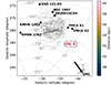 |
Fig. 1. Positions of the LMC age gap clusters. Grey dots indicate the locations of clusters and associations cataloged by Bica et al. (2008). Large circles indicate the positions of age gap clusters with the colors indicating their respective distances (the references for the ages are presented in Table A.2). The black arrow in the bottom right corner points towards the SMC. |
In Fig. 2 we compare the ages and metallicities of all age gap clusters for which both parameters were available in the literature. Additionally, Table A.2 compiles astrophysical parameters for other clusters in this age range. When looking at the other two clusters with ages compatible with SL 2, i.e., KMHK 1592 and ESO 121-03, we see that they all have similar metallicities.
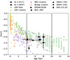 |
Fig. 2. Age-metallicity relation for age gap clusters. The blue pentagon and red hexagon indicate the results for the characterization of SL 2 using different grids of stellar evolution models. The black-filled points refer to other age gap clusters (see Table A.2 for references). Hollow points refer to different samples of the Magellanic System: the green circles refer to different field populations in the LMC analyzed by Piatti et al. (2012), the olive triangles to LMC star clusters analyzed by Narloch et al. (2022), the purple squares refer to a heterogeneous compilation of SMC star clusters gathered by Bica et al. (2022, and references therein), plus the results from Saroon et al. (2023), and the orange diamonds indicate the results for Magellanic Bridge star clusters characterized by Oliveira et al. (2023). Black-dashed lines show the edges of the age gap: at 4 and 10 Gyr. |
The figure also shows, for comparison, the age-metallicity relation (AMR) of LMC field star populations and stellar clusters, of SMC star clusters, as well as Magellanic Bridge star clusters. We see that in the age range of SL 2, the three regions have similar metallicities, compatible to the values for this cluster.
Finally, we investigated the mass of SL 2, following the method previously applied by the VISCACHA collaboration in Santos et al. (2020), Bica et al. (2022). We started by using the values of distance and color excess determined earlier to convert the measured integrated apparent magnitudes of SL 2 into absolute magnitudes. The values are presented in Table 1. They were then used for estimating the cluster mass by using the evolution of the mass-luminosity ratio for simple stellar populations developed by Maia et al. (2014):
![Mathematical equation: $$ \begin{aligned} \log (\mathcal{M} /\mathcal{M} _\odot ) = a + b \log \text{ Age}\text{[Gyr]} - 0.4 (M - M_\odot ), \end{aligned} $$](/articles/aa/full_html/2025/03/aa53506-24/aa53506-24-eq2.gif) (2)
(2)
where M and M⊙ are the absolute magnitudes of the cluster and the Sun, respectively, while ℳ refers to the mass, and a and b are coefficients that depend on the photometric band and metallicity of the cluster. For this work, we adopted the values of (a, b)V = ( − 5.87 ± 0.07, 0.608 ± 0.008) and (a, b)I = ( − 4.80 ± 0.10, 0.49 ± 0.01), determined for a metallicity of [Fe/H]= − 0.58, which is the smallest value provided by the authors.
We note that this metallicity is not representative of the values determined for SL 2. Still, for both V and I bands, the impact of metallicity on the final mass estimates is negligible and within uncertainties. The mass values for each band are presented in Table 1, together with the average between the two, which we have taken as the final mass for this cluster. The results from PARSEC-COLIBRI and MIST isochrones are in agreement with one another.
In Fig. 3, we show the age-mass relation of LMC, SMC, and Magellanic Bridge star clusters and compare it to the value measured for SL 2 using the PARSEC-COLIBRI isochrones. The compiled data for the LMC reveals that clusters older than ∼12 Gyr have masses of ∼105.5 ℳ⊙. For clusters with ages between 1 ∼ 4 Gyr, there is a large mass dispersion between 103.5 ∼ 105.5 ℳ⊙. Finally, for clusters younger than 1 Gyr, the masses stabilize around ≲104 ℳ⊙.
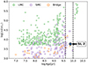 |
Fig. 3. Mass-age relation for star clusters. The hollow-green circles correspond to the heterogeneous compilation from Baumgardt et al. (2013, and references therein) for LMC star clusters. The hollow-purple squares show a similar compilation for the SMC, from Bica et al. (2022, and references therein). The hollow-orange diamonds refer to the characterization of Bridge clusters by Oliveira et al. (2023). The result for SL 2 from this work using PARSEC-COLIBRI isochrones is highlighted in the figure. The two black-dashed lines show the ages of 4 and 10 Gyr (the same as shown in Fig. 2), serving as limit indicators of the age gap. |
Naturally, there is an observational bias in the distributions observed in the figure. In particular, less massive clusters are more difficult to detect. For clusters older than 1 Gyr, the mass threshold increases with age, as a direct consequence of stellar evolution. This mass limit varies between the compilations of Bica et al. (2022), for the SMC, and Baumgardt et al. (2013), for the LMC, which explains why the former contains more clusters less massive than ≲103.5 M⊙ than the latter.
Even so, it is worth noting that SL 2 occupies a unique position in the mass-age relation, having a mass comparable to the younger clusters while being well-centered in the age gap. Although mass determinations for other age gap clusters are currently unavailable, their sizes, number of stars, and CMDs suggest that most of them would likely occupy a similar position in the age-mass relation as SL 2. More specifically, we would not expect any of them to reach the masses of the most massive clusters observed for ages larger than 10 Gyr – or marginally younger than 4 Gyr. This is in agreement with the discussion presented by Balbinot et al. (2010), who argued that since the age gap is not present in field stars, such feature may be less pronounced among low mass (≲104 M⊙) clusters.
4. Discussion
Piatti (2022) previously discussed potential origins for the age gap clusters presenting two possible scenarios: (i) these clusters were formed in the LMC or (ii) they were formed outside the LMC and were accreted by the galaxy from an external source, whether it was as part of a merger event with a dwarf galaxy or from tidal stripping from the SMC. The author argues that external formation would be more likely, unless more clusters were found to be in the age range between 6 and 10 Gyr. As such, the characterization of SL 2 presented in this letter could contribute to the in situ scenario, especially considering the consistency between the age and metallicity of the clusters in this age range with the field stars of the LMC. However, this does not offer definitive proof.
Arguing in favor of the ex situ formation, Carpintero et al. (2013) presented a set of orbital simulations between the LMC and SMC and showed that depending on the orbit eccentricity, it is possible that about 15% of the SMC clusters would be expelled from this galaxy and accreted by the LMC. The authors explain that this could explain the small number of clusters with ages older than ∼7 Gyr in the SMC. Consequently, the LMC cluster population older than 7 Gyr would (at least partially) be composed of objects formed in the SMC. Combining this with the fact that it is possible to find regions in the SMC and the Bridge where the age-metallicity relation of both field stars and clusters are also compatible with the values measured for the age gap clusters (as seen in Fig. 2 and also Carrera et al. 2008; Dobbie et al. 2014; Oliveira et al. 2023; Saroon et al. 2023) would make the external formation scenario plausible.
If the age gap clusters had indeed been formed in situ during the quiescent period of the LMC, the comparative lack of massive clusters observed in Fig. 3 requires an explanation, whether based the assumption that the clusters were formed with typically smaller masses and/or that they suffered from stronger dynamical dissolution. Possibly, a combination of these two phenomena could have been at play: from the description of the mass dissolution rate for star clusters from Lamers et al. (2010), objects with a smaller initial mass would be expected to dissolve faster. As for the ex situ explanation, as can be seen in Fig. 3, the mass of SL 2 is within the expected interval of masses for older clusters in the SMC and Bridge, which could support the hypothesis that SL 2 (and, potentially, other age gap clusters) have originated in the SMC and later were accreted by the LMC.
In the future, a spectroscopic follow-up for SL 2 would allow for understanding its kinematics (for instance, using the calcium triplet technique in low-resolution spectra, as done by the VISCACHA collaboration in Dias et al. 2021, 2022; Parisi et al. 2024). Additionally, observations with deeper photometry could be used to better understand the excess of bluer stars in its lower main sequence and evaluate the mass function of the cluster, which could be used to investigate if it is expected to have suffered significant dissolution. These types of observations would also benefit studies of other age gap clusters, allowing for a homogenous and complete characterization of these objects.
Finally, we highlight that SL 2 is a cluster known to the astronomical community for decades, but it could only be characterized as part of the age gap due largely to ground-based surveys in middle-sized telescopes such as VISCACHA. The same also applies to DES (which led to the identification of NGC 1997 as an age gap cluster and the discovery of DES001SC04, by Pieres et al. 2016) and YMCA (with the analysis of KMHK 1762 and the discovery of the candidates YMCA 53 and YMCA 61 by Gatto et al. 2022, 2024). As such, this is an important example of how these surveys are leading towards a more comprehensive understanding of the Magellanic Clouds.
The code is publicly available at https://github.com/Bereira/SIESTA/
Acknowledgments
The members of the VISCACHA survey acknowledge the excellence of Paola Marigo’s work with PARSEC-COLIBRI stellar evolutionary models and express their deep regret for her passing last October. The authors thank the anonymous referee for the comments and suggestions for this letter. BPLF acknowledges financial support from Conselho Nacional de Desenvolvimento Científico e Tecnológico (CNPq, Brazil; proc. 140642/2021-8) and Coordenação de Aperfeiçoamento de Pessoal de Nível Superior (CAPES, Brazil; Finance Code 001; proc. 88887.935756/2024-00). BD acknowledges support by ANID-FONDECYT iniciación grant No. 11221366 and from the ANID Basal project FB210003. FFSM acknowledges financial support from FAPERJ (proc. E-26/201.386/2022 and E-26/211.475/2021). TA acknowledges CNPQ (proc. 201146/2017-7). This material is based upon work supported by the National Science Foundation under Cooperative Agreement 1258333 managed by the Association of Universities for Research in Astronomy (AURA), and the Department of Energy under Contract No. DE-AC02-76SF00515 with the SLAC National Accelerator Laboratory. Additional funding for Rubin Observatory comes from private donations, grants to universities, and in-kind support from LSSTC Institutional Members.” SOS. acknowledges the DGAPA-PAPIIT grant IA103224 and the support from Nadine Neumayer’s Lise Meitner grant from the Max Planck Society. OKS acknowledges partial financial support by UESC (proc. 073.11157.2022.0033250-38) This research was financed in part by CAPES. The authors acknowledge financial support from CNPq (proc. 404482/2021-0). Based on observations obtained at the Southern Astrophysical Research (SOAR) telescope, which is a joint project of the Ministério da Ciência, Tecnologia e Inovações (MCTI/LNA) do Brasil, the US National Science Foundation’s NOIRLab, the University of North Carolina at Chapel Hill (UNC), and Michigan State University (MSU).
References
- Balbinot, E., Santiago, B. X., Kerber, L. O., Barbuy, B., & Dias, B. M. S. 2010, MNRAS, 404, 1625 [NASA ADS] [Google Scholar]
- Baumgardt, H., Parmentier, G., Anders, P., & Grebel, E. K. 2013, MNRAS, 430, 676 [NASA ADS] [CrossRef] [Google Scholar]
- Bekki, K., & Chiba, M. 2005, MNRAS, 356, 680 [NASA ADS] [CrossRef] [Google Scholar]
- Bekki, K., Couch, W. J., Beasley, M. A., et al. 2004, ApJ, 610, L93 [NASA ADS] [CrossRef] [Google Scholar]
- Bica, E., Bonatto, C., Dutra, C. M., & Santos, J. F. C. 2008, MNRAS, 389, 678 [Google Scholar]
- Bica, E., Maia, F. F. S., Oliveira, R. A. P., et al. 2022, MNRAS, 517, L41 [NASA ADS] [CrossRef] [Google Scholar]
- Bressan, A., Marigo, P., Girardi, L., et al. 2012, MNRAS, 427, 127 [NASA ADS] [CrossRef] [Google Scholar]
- Cardelli, J. A., Clayton, G. C., & Mathis, J. S. 1989, ApJ, 345, 245 [Google Scholar]
- Carpintero, D. D., Gomez, F. A., & Piatti, A. E. 2013, MNRAS, 435, L63 [NASA ADS] [CrossRef] [Google Scholar]
- Carrera, R., Gallart, C., Hardy, E., Aparicio, A., & Zinn, R. 2008, AJ, 135, 836 [NASA ADS] [CrossRef] [Google Scholar]
- Chatterjee, S., Umbreit, S., Fregeau, J. M., & Rasio, F. A. 2013, MNRAS, 429, 2881 [NASA ADS] [CrossRef] [Google Scholar]
- Choi, J., Dotter, A., Conroy, C., et al. 2016, ApJ, 823, 102 [Google Scholar]
- de Grijs, R., & Bono, G. 2015, AJ, 149, 179 [Google Scholar]
- de Grijs, R., Wicker, J. E., & Bono, G. 2014, AJ, 147, 122 [Google Scholar]
- Dias, B., Maia, F., Kerber, L., et al. 2020, in Star Clusters: From the Milky Way to the Early Universe, eds. A. Bragaglia, M. Davies, A. Sills, & E. Vesperini, IAU Symp., 351, 89 [NASA ADS] [Google Scholar]
- Dias, B., Angelo, M. S., Oliveira, R. A. P., et al. 2021, A&A, 647, L9 [NASA ADS] [CrossRef] [EDP Sciences] [Google Scholar]
- Dias, B., Parisi, M. C., Angelo, M., et al. 2022, MNRAS, 512, 4334 [NASA ADS] [CrossRef] [Google Scholar]
- Dobbie, P. D., Cole, A. A., Subramaniam, A., & Keller, S. 2014, MNRAS, 442, 1680 [NASA ADS] [CrossRef] [Google Scholar]
- Donada, J., Anders, F., Jordi, C., et al. 2023, A&A, 675, A89 [NASA ADS] [CrossRef] [EDP Sciences] [Google Scholar]
- Dotter, A. 2016, ApJS, 222, 8 [Google Scholar]
- Ferreira, B. P. L., Santos, J. F. C. Jr, Dias, B., et al. 2024, MNRAS, 533, 4210 [NASA ADS] [CrossRef] [Google Scholar]
- Gardin, J. F., Santos, J. F. C., Maia, F. F. S., et al. 2024, MNRAS, 532, 1683 [NASA ADS] [CrossRef] [Google Scholar]
- Gatto, M., Ripepi, V., Bellazzini, M., et al. 2020, MNRAS, 499, 4114 [Google Scholar]
- Gatto, M., Ripepi, V., Bellazzini, M., et al. 2022, A&A, 664, L12 [NASA ADS] [CrossRef] [EDP Sciences] [Google Scholar]
- Gatto, M., Ripepi, V., Bellazzini, M., et al. 2024, A&A, 690, A164 [NASA ADS] [CrossRef] [EDP Sciences] [Google Scholar]
- Harris, J., & Zaritsky, D. 2009, AJ, 138, 1243 [NASA ADS] [CrossRef] [Google Scholar]
- Jensen, J., Mould, J., & Reid, N. 1988, ApJS, 67, 77 [NASA ADS] [CrossRef] [Google Scholar]
- Kerber, L. O., Santiago, B. X., & Brocato, E. 2007, A&A, 462, 139 [NASA ADS] [CrossRef] [EDP Sciences] [Google Scholar]
- King, I. 1962, AJ, 67, 471 [Google Scholar]
- Lada, C. J., & Lada, E. A. 2003, ARA&A, 41, 57 [Google Scholar]
- Lamers, H. J. G. L. M., Baumgardt, H., & Gieles, M. 2010, MNRAS, 409, 305 [CrossRef] [Google Scholar]
- Lynga, G., & Westerlund, B. E. 1963, MNRAS, 127, 31 [CrossRef] [Google Scholar]
- Mackey, A. D., Payne, M. J., & Gilmore, G. F. 2006, MNRAS, 369, 921 [NASA ADS] [CrossRef] [Google Scholar]
- Maia, F. F. S., Corradi, W. J. B., & Santos, J. F. C. Jr 2010, MNRAS, 407, 1875 [NASA ADS] [CrossRef] [Google Scholar]
- Maia, F. F. S., Piatti, A. E., & Santos, J. F. C. 2014, MNRAS, 437, 2005 [Google Scholar]
- Maia, F. F. S., Dias, B., Santos, J. F. C., et al. 2019, MNRAS, 484, 5702 [Google Scholar]
- Marigo, P., Girardi, L., Bressan, A., et al. 2017, ApJ, 835, 77 [Google Scholar]
- Massana, P., Ruiz-Lara, T., Noël, N. E. D., et al. 2022, MNRAS, 513, L40 [CrossRef] [Google Scholar]
- Mateo, M., Hodge, P., & Schommer, R. A. 1986, ApJ, 311, 113 [NASA ADS] [CrossRef] [Google Scholar]
- Milone, A. P., Cordoni, G., Marino, A. F., et al. 2023, A&A, 672, A161 [NASA ADS] [CrossRef] [EDP Sciences] [Google Scholar]
- Narloch, W., Pietrzyński, G., Gieren, W., et al. 2022, A&A, 666, A80 [NASA ADS] [CrossRef] [EDP Sciences] [Google Scholar]
- O’Donnell, J. E. 1994, ApJ, 422, 158 [Google Scholar]
- Oliveira, R. A. P., Maia, F. F. S., Barbuy, B., et al. 2023, MNRAS, 524, 2244 [NASA ADS] [CrossRef] [Google Scholar]
- Olszewski, E. W., Schommer, R. A., Suntzeff, N. B., & Harris, H. C. 1991, AJ, 101, 515 [Google Scholar]
- Parisi, M. C., Geisler, D., Clariá, J. J., et al. 2015, AJ, 149, 154 [Google Scholar]
- Parisi, M. C., Oliveira, R. A. P., Angelo, M. S., et al. 2024, MNRAS, 527, 10632 [Google Scholar]
- Piatti, A. E. 2021, AJ, 161, 199 [NASA ADS] [CrossRef] [Google Scholar]
- Piatti, A. E. 2022, MNRAS, 511, L72 [NASA ADS] [CrossRef] [Google Scholar]
- Piatti, A. E., & Geisler, D. 2013, AJ, 145, 17 [Google Scholar]
- Piatti, A. E., Sarajedini, A., Geisler, D., Bica, E., & Clariá, J. J. 2002, MNRAS, 329, 556 [NASA ADS] [CrossRef] [Google Scholar]
- Piatti, A. E., Geisler, D., & Mateluna, R. 2012, AJ, 144, 100 [NASA ADS] [CrossRef] [Google Scholar]
- Pieres, A., Santiago, B., Balbinot, E., et al. 2016, MNRAS, 461, 519 [NASA ADS] [CrossRef] [Google Scholar]
- Rich, R. M., Shara, M. M., & Zurek, D. 2001, AJ, 122, 842 [Google Scholar]
- Santos, J. F. C. Jr, Maia, F. F. S., Dias, B., et al. 2020, MNRAS, 498, 205 [NASA ADS] [CrossRef] [Google Scholar]
- Sarajedini, A. 1998, AJ, 116, 738 [NASA ADS] [CrossRef] [Google Scholar]
- Saroon, S., Dias, B., Tsujimoto, T., et al. 2023, A&A, 677, A35 [NASA ADS] [CrossRef] [EDP Sciences] [Google Scholar]
- Schlegel, D. J., Finkbeiner, D. P., & Davis, M. 1998, ApJ, 500, 525 [Google Scholar]
- Shapley, H., & Lindsay, E. M. 1963, Ir. Astron. J., 6, 74 [Google Scholar]
- Skowron, D. M., Skowron, J., Udalski, A., et al. 2021, ApJS, 252, 23 [Google Scholar]
- The Dark Energy Survey Collaboration 2005, arXiv e-prints [arXiv:astro-ph/0510346] [Google Scholar]
- Tokovinin, A., Cantarutti, R., Tighe, R., et al. 2016, PASP, 128, 125003 [NASA ADS] [CrossRef] [Google Scholar]
- Weisz, D. R., Dolphin, A. E., Skillman, E. D., et al. 2013, MNRAS, 431, 364 [Google Scholar]
- Zocchi, A., Gieles, M., Hénault-Brunet, V., & Varri, A. L. 2016, MNRAS, 462, 696 [Google Scholar]
Appendix A: Additional material
Observations of SL 2.
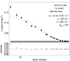 |
Fig. A.1. In the top panel, black diamonds represent the radial density profile evaluated for SL 2, and the dashed line shows the fitted King (1962) function. The dotted lines represent the functions within 1-σ of the best fit. The bottom panel displays the fit residuals. |
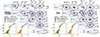 |
Fig. A.2. Results from the CMD fitting using PARSEC+COLIBRI isochrones (top) and MIST isochrones (bottom). For each figure, the panels on the top right show the marginalized probability distribution of each pair of fitted parameters. In the main diagonal, the 1D marginalizations are shown as histograms, while the dotted lines represent the priors, and the blue, continuous line indicates the fitted skewed-normal distribution used for inferring the final parameters. In the bottom left panels, the CMDs of the best-fitting synthetic population are shown (hollowed, orange points), together with the corresponding isochrone (dashed, black line) and the observed CMD (filled, green points). |
Astrophysical parameters of clusters in the LMC age gap. The age determination of ESO 121-03 from Mackey et al. (2006) is presented as a range, as the authors express it. For the metallicities of YMCA 53 and YMC 61, Gatto et al. (2024) use the expected values from the age-metallicity relation determined by Piatti & Geisler (2013), Parisi et al. (2015). For YMCA 53, YMCA 61, and KMHK 1592, the assumed distance is the same as of the center of the LMC (de Grijs et al. 2014). Milone et al. (2023) estimated uncertainties only for specific clusters as indicators of the precision of their analysis. We adopted the values from Kron 1, which had the closest age to the determination for SL 2, in the same work.
Appendix B: Decontamination process
Since reliable astrometric and spectroscopic information is lacking for this cluster, we used the photometric method to estimate membership probabilities described in Maia et al. (2010). We start by separating the observed stars into two distinct regions. The first one corresponds to the cluster region, which is defined as a 42.5″ circle around the cluster center. The second region corresponds to the field and is defined as all stars within the field of view that fall outside a circle of 85″ around the cluster center. The sizes of both regions were defined based on the tidal radius fitted previously. By choosing an inner radius of half the tidal radius, we increase the ratio of cluster-to-field stars, which makes the decontamination process more reliable, while losing proportionally few cluster stars (about 16%, as predicted by integrating Eq. 1).
The decontamination method works by comparing two-dimensional histograms of the CMDs from the inner and outer regions and then assigning membership probabilities to every star in the inner region based on the relative number of stars in each bin (normalized by the areas of their respective regions) and the distance of each star from the cluster center. This process is repeated iteratively, varying the sizes and positions of the histogram bins, and producing different membership probabilities for each star. These values are later averaged, and some statistical considerations regarding the different probabilities of each iteration are done to filter the stars that, most likely, belong to the cluster. In Fig. B.1 we can see the two regions defined for the membership determination, as well as the final CMD obtained after the removal of the contribution from field stars.
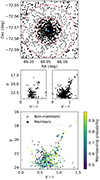 |
Fig. B.1. Top: Distribution of stars in the observed field. The two circles mark the limits of the regions used for decontamination: stars inside the inner circle are part of the cluster region, and stars outside the outer circle are all assigned to the field. Middle: The corresponding CMDs. Bottom: Decontaminated CMD of the inner region. Filled, colored circles are considered members (with membership probabilities indicated by the color bar), and hollow, black circles are discarded as field stars. |
Appendix C: CMD fitting with distance priors
The large distance obtained for SL 2 is unusual for an LMC cluster. Given the scientific context in which this cluster is inserted, it is essential to ensure that the parameters determined from isochrone fitting are reliable. Looking at the posterior probability distributions presented in Fig. A.2, we do not see signs of another, statistically significant possible solution for SL 2. The comparison between the best-fitting synthetic population and the observations also shows that the parameters constrain well the main properties of the CMD.
Still, to search for possible degeneracies, we repeat the characterization adopting a Gaussian distance prior around the LMC center, with a standard deviation of 1.0 kpc. The new results, obtained from this prior, are shown in Table C.1 and, in Fig. C.1, we show a comparison between the best-fitting solutions with and without the included prior. From the figure, we see that the new solutions are good matches to the MSTO and the red giant branch of the cluster. However, they do not match the subgiant branch and the RC as well as the best-fit obtained by using uninformative distance priors, being, for both isochrone grids, slightly brighter than what is observed for the cluster.
Looking at the values in Table C.1, we observe that the ages obtained in the new solutions are between 1 to 1.5 Gyr older than the previous solutions. Still, the values are consistent with those of a genuine age gap cluster. The masses of the cluster are also smaller but with values compatible with the previous determinations, with differences smaller than the uncertainty intervals. Therefore, the discussion presented in this letter regarding these two parameters, as well as the classification of SL 2 as an age gap would remain unchanged, even if this new solution were to be adopted.
Nonetheless, the color excess obtained in the new solutions is significantly smaller than what is expected from the dust maps from Schlegel et al. (1998). Additionally, the metallicities are much larger than the values obtained with an uninformative distance prior. If these values were to be considered correct, SL 2 would be an outlier in the age metallicity relation, having values that are discrepant from both other age gap clusters of similar age, and the LMC field star population (see Fig. 2).
These differences, combined with the fact that the CMD best-fitting solutions are worse matches to the observations, lead to the conclusion that the solution with uninformative distance priors, presented in Table 1 and discussed in this letter are the most adequate ones.
Astrophysical parameters determined in this work for SL 2, with the addition of a distance prior.
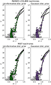 |
Fig. C.1. Top two panels: Comparison between the observed, decontaminated CMD of SL 2 (gray points) and the best-fitting synthetic CMD obtained from PARSEC-COLIBRI isochrones with a non-informative distance prior (left, green diamonds) and a Gaussian distance prior (right, purple squares). Bottom two panels: Same but with MIST isochrones. The isochrone used for generating the synthetic CMD is shown as the black line in all panels. |
All Tables
Astrophysical parameters of clusters in the LMC age gap. The age determination of ESO 121-03 from Mackey et al. (2006) is presented as a range, as the authors express it. For the metallicities of YMCA 53 and YMC 61, Gatto et al. (2024) use the expected values from the age-metallicity relation determined by Piatti & Geisler (2013), Parisi et al. (2015). For YMCA 53, YMCA 61, and KMHK 1592, the assumed distance is the same as of the center of the LMC (de Grijs et al. 2014). Milone et al. (2023) estimated uncertainties only for specific clusters as indicators of the precision of their analysis. We adopted the values from Kron 1, which had the closest age to the determination for SL 2, in the same work.
Astrophysical parameters determined in this work for SL 2, with the addition of a distance prior.
All Figures
|
Fig. 1. Positions of the LMC age gap clusters. Grey dots indicate the locations of clusters and associations cataloged by Bica et al. (2008). Large circles indicate the positions of age gap clusters with the colors indicating their respective distances (the references for the ages are presented in Table A.2). The black arrow in the bottom right corner points towards the SMC. |
| In the text | |
|
Fig. 2. Age-metallicity relation for age gap clusters. The blue pentagon and red hexagon indicate the results for the characterization of SL 2 using different grids of stellar evolution models. The black-filled points refer to other age gap clusters (see Table A.2 for references). Hollow points refer to different samples of the Magellanic System: the green circles refer to different field populations in the LMC analyzed by Piatti et al. (2012), the olive triangles to LMC star clusters analyzed by Narloch et al. (2022), the purple squares refer to a heterogeneous compilation of SMC star clusters gathered by Bica et al. (2022, and references therein), plus the results from Saroon et al. (2023), and the orange diamonds indicate the results for Magellanic Bridge star clusters characterized by Oliveira et al. (2023). Black-dashed lines show the edges of the age gap: at 4 and 10 Gyr. |
| In the text | |
|
Fig. 3. Mass-age relation for star clusters. The hollow-green circles correspond to the heterogeneous compilation from Baumgardt et al. (2013, and references therein) for LMC star clusters. The hollow-purple squares show a similar compilation for the SMC, from Bica et al. (2022, and references therein). The hollow-orange diamonds refer to the characterization of Bridge clusters by Oliveira et al. (2023). The result for SL 2 from this work using PARSEC-COLIBRI isochrones is highlighted in the figure. The two black-dashed lines show the ages of 4 and 10 Gyr (the same as shown in Fig. 2), serving as limit indicators of the age gap. |
| In the text | |
|
Fig. A.1. In the top panel, black diamonds represent the radial density profile evaluated for SL 2, and the dashed line shows the fitted King (1962) function. The dotted lines represent the functions within 1-σ of the best fit. The bottom panel displays the fit residuals. |
| In the text | |
|
Fig. A.2. Results from the CMD fitting using PARSEC+COLIBRI isochrones (top) and MIST isochrones (bottom). For each figure, the panels on the top right show the marginalized probability distribution of each pair of fitted parameters. In the main diagonal, the 1D marginalizations are shown as histograms, while the dotted lines represent the priors, and the blue, continuous line indicates the fitted skewed-normal distribution used for inferring the final parameters. In the bottom left panels, the CMDs of the best-fitting synthetic population are shown (hollowed, orange points), together with the corresponding isochrone (dashed, black line) and the observed CMD (filled, green points). |
| In the text | |
|
Fig. B.1. Top: Distribution of stars in the observed field. The two circles mark the limits of the regions used for decontamination: stars inside the inner circle are part of the cluster region, and stars outside the outer circle are all assigned to the field. Middle: The corresponding CMDs. Bottom: Decontaminated CMD of the inner region. Filled, colored circles are considered members (with membership probabilities indicated by the color bar), and hollow, black circles are discarded as field stars. |
| In the text | |
|
Fig. C.1. Top two panels: Comparison between the observed, decontaminated CMD of SL 2 (gray points) and the best-fitting synthetic CMD obtained from PARSEC-COLIBRI isochrones with a non-informative distance prior (left, green diamonds) and a Gaussian distance prior (right, purple squares). Bottom two panels: Same but with MIST isochrones. The isochrone used for generating the synthetic CMD is shown as the black line in all panels. |
| In the text | |
Current usage metrics show cumulative count of Article Views (full-text article views including HTML views, PDF and ePub downloads, according to the available data) and Abstracts Views on Vision4Press platform.
Data correspond to usage on the plateform after 2015. The current usage metrics is available 48-96 hours after online publication and is updated daily on week days.
Initial download of the metrics may take a while.