| Issue |
A&A
Volume 590, June 2016
|
|
|---|---|---|
| Article Number | A3 | |
| Number of page(s) | 17 | |
| Section | Extragalactic astronomy | |
| DOI | https://doi.org/10.1051/0004-6361/201527081 | |
| Published online | 28 April 2016 | |
Modelling the number density of Hα emitters for future spectroscopic near-IR space missions
1
INAF – Osservatorio Astronomico di Bologna, via Ranzani
1, 40127
Bologna,
Italy
e-mail:
This email address is being protected from spambots. You need JavaScript enabled to view it.
2
Center for Cosmology and Astroparticle Physics, The Ohio State
University, 191 West Woodruff
Lane, Columbus,
Ohio
43210,
USA
3
Centre for Astrophysics Research, Science and Technology Research
Institute, University of Hertfordshire, Hatfield, AL10 9AB, UK
4
Dipartimento di Fisica e Astronomia, Università di
Bologna, viale Berti Pichat
6/2, 40127
Bologna,
Italy
5
Institute for Computational Cosmology (ICC), Department of
Physics, Durham University, South
Road, Durham,
DH1 3LE,
UK
6
Department of Physics and Astronomy, University College
London, Gower
Street, London,
WC1E 6BT,
UK
Received: 29 July 2015
Accepted: 16 February 2016
Abstract
Context. The future space missions Euclid and WFIRST-AFTA will use the Hα emission line to measure the redshifts of tens of millions of galaxies. The Hα luminosity function at z> 0.7 is one of the major sources of uncertainty in forecasting cosmological constraints from these missions.
Aims. We construct unified empirical models of the Hα luminosity function spanning the range of redshifts and line luminosities relevant to the redshift surveys proposed with Euclid and WFIRST-AFTA.
Methods. By fitting to observed luminosity functions from Hα surveys, we build three models for its evolution. Different fitting methodologies, functional forms for the luminosity function, subsets of the empirical input data, and treatment of systematic errors are considered to explore the robustness of the results.
Results. Functional forms and model parameters are provided for all three models, along with the counts and redshift distributions up to z ~ 2.5 for a range of limiting fluxes (FHα> 0.5 − 3 × 10-16 erg cm-2 s-1) that are relevant for future space missions. For instance, in the redshift range 0.90 <z< 1.8, our models predict an available galaxy density in the range 7700–130 300 and 2000–4800 deg-2 respectively at fluxes above FHα> 1 and 2 × 10-16 erg cm-2 s-1, and 32 000–48 0000 for FHα> 0.5 × 10⁻¹⁶ erg cm-2 s-1 in the extended redshift range 0.40 <z< 1.8. We also consider the implications of our empirical models for the total Hα luminosity density of the Universe, and the closely related cosmic star formation history.
Key words: galaxies: evolution / galaxies: high-redshift / galaxies: star formation / galaxies: luminosity function, mass function / cosmology: observations
© ESO, 2016
1. Introduction
Since the discovery of the apparent acceleration of the expansion of the Universe (e.g. Riess et al. 1998; Perlmutter et al. 1999), many efforts have been made to measure the dark energy equation of state, exploiting different observations. Among the suggestions proposed, the use of baryon acoustic oscillations (BAO) as standard rulers appears to have a particularly low level of systematic uncertainty since it corresponds to a feature in the correlation function, whereas most observational and astrophysical systematics are expected to be broad-band (e.g. Albrecht et al. 2006). Indeed, in recent years, the BAO technique has seen a dramatic improvement in capability owing to the increase in volume probed by galaxy surveys (e.g. Cole et al. 2005; Glazebrook et al. 2005; Eisenstein et al. 2005; Percival et al. 2007, 2010; Blake et al. 2011a,b; Padmanabhan et al. 2012; Xu et al. 2012; Kazin et al. 2013, 2014; Anderson et al. 2014).
The future space-based galaxy redshift surveys planned for the ESA’s Euclid (Laureijs et al. 2011) and NASA’s Wide-Field Infrared Survey Telescope – Astrophysics Focused Telescope Assets design (WFIRST-AFTA; Spergel et al. 2015b; Green et al. 2012) missions will use near-IR (NIR) slitless spectroscopy to collect large samples of emission-line galaxies to probe dark energy. These spectroscopic surveys will identify mainly Hα emitters out as far as z ~ 2, and their maps of large-scale structure will be used for studies of BAO, power spectrum P(k) in general, large-scale structure, as well as other statistics such as the measurement of the rate of growth of structure using redshift space distortions (Kaiser 1987; Guzzo et al. 2008). In this context the space density of Hα emitters (i.e. their luminosity function) is a key ingredient for a mission’s performance forecast to determine the number of objects above the mission’s sensitivity threshold and optimize the survey.
It is known that the cosmic star formation rate was higher in the Universe’s past than it is today, possibly peaking near z ~ 2 (Madau & Dickinson 2014), thereby ensuring a high number of star-forming objects with high luminosity at high redshift suitable for BAO measurements. However, the abundance of Hα emitters detectable by blind spectroscopy has historically been firmly established only at low redshift by means of spectroscopic surveys in the optical (e.g. Gallego et al. 1995). At higher redshift, from the ground, the intense airglow makes NIR spectroscopic searches for emission line galaxies impractical; thus systematic ground-based NIR Hα spectroscopic searches in early studies have been limited to small areas with single slit spectroscopy (e.g. Tresse et al. 2002). Therefore, narrow-band NIR searches have been used as an alternative method for identifying large numbers of z> 0.7 emission-line galaxies, e.g. HiZELS (Geach et al. 2008; Sobral et al. 2009, 2012, 2013) and the NEWFIRM Hα Survey (Ly et al. 2011). These surveys have the advantage of wide area and high sensitivity to emission lines but suffer from their narrow redshift ranges and significant contamination from emission lines at different redshifts. From space, grism spectroscopy with NICMOS (Yan et al. 1999; Shim et al. 2009) and more recently with the Wide Field Camera 3 (WFC3) on the Hubble Space Telescope (HST), have allowed small-area surveys, such as the WFC3 Infrared Spectroscopic Parallels (WISP) survey (Colbert et al. 2013), at relevant fluxes (deeper than Euclid or WFIRST-AFTA) to probe the luminosity function of emission line objects at high redshift.
As a result, early studies of space-based galaxy redshift surveys often based their Hα luminosity function models on indirect extrapolations from alternative star formation indicators such as the rest-frame ultraviolet continuum or [O ii] line strength (e.g. Ly et al. 2007; Takahashi et al. 2007; Reddy et al. 2008). While physically motivated, this procedure suffers from a multitude of uncertainties in the details of the H ii region parameters, dust extinction, stellar populations, and the joint distribution thereof, and the impact of uncertainties in the predicted Hα flux is enhanced by the steepness of the luminosity function.
Motivated by the prospect of future dark energy surveys targeting Hα emitters at NIR wavelengths (i.e. z> 0.5), Geach et al. (2010) used the empirical data available at that time to model the evolution of the Hα luminosity function out to z ~ 2. Much more ground- and space-based data have become available since then, thanks largely to the same improvements in NIR detector technology that make Euclid and WFIRST-AFTA possible. In particular, the WFC3 Infrared Spectroscopic Parallels (WISP) survey (Colbert et al. 2013) has enabled the blind detection of large numbers of Hα emitters. Due to its similarity to the observational setups planned for Euclid and WFIRST-AFTA, it is an excellent test case against which to calibrate expectations for these future missions.
In this work, we update the empirical model of Geach et al. (2010), collecting a larger dataset of Hα luminosity functions from low- to high-redshift, in order to constrain the evolution of the space density of Hα emitters. We construct three empirical models and make prediction for future Hα surveys as a function of sensitivity threshold (i.e. counts) and redshift (i.e. redshift distributions). We scale all the luminosity functions to a reference cosmology with H0 = 70 km s-1 Mpc-1 and Ωm = 0.3, and present results in terms of comoving volume. The models and luminosity functions presented here are for Hα only, not Hα+[N ii]. The final aim of these models is to provide key inputs for instrumental simulations essential to derive forecast in future space missions, like Euclid and WFIRST-AFTA, that at the nominal resolution will be partially able to resolve Hα. Future simulations will clarify all the observational effects, from source confusion to the [N ii] contamination and percentiles of blended lines, completeness and selection effects.
We emphasize here that our models are empirical and therefore we have reduced as much as possible any astrophysics assumption, but those based on Hα public data. Furthermore, we do not attempt to exclude the AGN contribution from the bright end of the Hα public luminosity functions, being AGNs valid sources (as Hα emitters) for the current planned missions. Thus they should not be excluded to derive the total number of Hα emitters mapped by Euclid and WFIRST-AFTA.
This paper is organized as follows. The input data is described in Sect. 2. The three models and the procedures used to derive them are described in Sect. 3, and the comparison to the input data is summarized in Sect. 4. Section 5 describes the redshift and flux distribution, with a focus on the ranges relevant to Euclid and WFIRST-AFTA, and Sect. 6 compares our results to semi-analytic mock catalogues. Our Hα luminosity functions are compared to other estimates of the cosmic star formation history in Sect. 7. We conclude in Sect. 8. Technical details are placed in the appendices.
2. Empirical luminosity functions
Forecasts for future NIR slitless galaxy redshift surveys require as input the luminosity function of Hα emitters (HαLF) in order to determine the number of objects above the mission’s sensitivity threshold. In particular, we focus on the prediction for the originally planned Euclid Wide grism survey (Laureijs et al. 2011), i.e. to a flux limit FHα> 3 × 10-16 erg cm-2 s-1, and detectore sensitivity 1.1 <λ< 2.0 μm (sampling Hα at 0.70 <z< 2.0) over 15 000 deg2. A smaller area (2200 deg2) and a fainter flux limit (>1 × 10-16 erg cm-2 s-1) is the baseline depth of WFIRST-AFTA (Green et al. 2011) with a grism spanning the wavelength range 1.35 − 1.95μm.
The original predictions presented in the Euclid Definition Study Report (the Red Book, Laureijs et al. 2011) used the predicted counts of Hα emitters by Geach et al. (2010). This model was based on HST and other data available prior to 2010. Here, we provide an updated compilation of empirical Hα LFs available in literature, and use the most recent and verified ones out to zmax ~ 2.3 to build three updated models of Hα emitters counts. To provide precise predictions over the redshift range of interest of NIR missions (i.e. 0.7 <z< 2) all three models include estimates from the HiZELS narrow-band ground-based imaging survey with UKIRT, Subaru and VLT (Sobral et al. 2013), covering ~2 deg2 in the COSMOS field at z = 0.4,0.84,1.47,2.23; the WISP slitless space-based spectroscopic survey with HST+WFC3 (Colbert et al. 2013), sensitive to Hα in the range 0.7 <z< 1.5 up to faint flux levels (3 − 5 × 10-17 erg s-1 cm-2) on a small area (~0.037 deg2); and the grism survey with HST+NICMOS by Shim et al. (2009), on ~104 arcmin2 over the redshift range 0.7 <z< 1.9. To extend the models to a broader redshift range and better constrain the evolutionary form, we include other luminosity functions available at lower redshifts. Different subsets of input data are adopted in the three models to describe the evolution in redshift of the HαLF, as well as to explore the robustness of the predictions.
Empirical Schechter parameters for the various surveys considered, ordered by redshift.
Our focus is on predictions for the yield of galaxy redshift surveys, so we work in terms of observed Hα flux, i.e. with no correction for extinction in the target galaxy. Generally, in Hα surveys direct measurements of extinction are unavailable, and thus require purely statistical corrections. Usually an average extinction of 1 mag. has been adopted by most of the authors (see Hopkins 2004; Sobral et al. 2013). In cases where such corrections have been applied in the literature, we have undone the correction. Furthermore, in many of the input datasets, Hα is partially or fully blended with the [N ii] doublet, and the inference of separate Hα and [N ii] fluxes is based on different assumption on their ratio or on different scaling relation. The luminosity functions presented here are for Hα only, not Hα+[N ii], since future space missions, like Euclid and WFIRST-AFTA, will have higher spectral resolution than HST and will be partially able to resolve the Hα+[N ii] complex. The inferred Hα luminosity function is sensitive to the prescription for the [N ii] correction. In Appendix C we explore the effects of different treatments.
In Table 1 we list the compilation of HαLF Schechter parameters provided by various Hα surveys spanning the redshift range 0 <z< 2 which are used in this work. We also list the subset of data used in each model. Schechter parameters have been converted to the same cosmology and to the original Hα extincted luminosity, when necessary. The luminosities in HiZELS LFs have been further corrected for aperture. These corrections are based on the fraction of a Kolmogorov seeing disk of the specified size (0.9, 0.8, 0.8, or 0.8 arcsec, full width at half maximum, specified by Sobral et al. 2013) convolved with an exponential profile disk of half-light radius 0.3 arcsec. Similar correction has been adopted by Sobral et al. (2015a) within the same survey (see their Sect. 2.4). Variations of this procedure are explored in Appendix C, where we find a 10% change in the abundance of Hα emitters in the range relevant for Euclid if this correction is turned off entirely, and a 2% change if the measured size-flux relation (Colbert et al. 2013) is used in place of a single reference value.
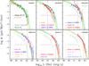 |
Fig. 1 Hα LFs at various redshifts. The dotted lines mark the nominal flux limit of Euclid (3 × 10-16 erg cm-2 s-1) in the lower bound of each redshift range. Observed Schechter LFs are shown as thin lines and squares in the observed luminosity range and listed in the labels. For comparison, the LFs from Empirical Models 1, 2, and 3 are shown (in yellow, cyan, and pink, respectively) as thick lines in the same redshift range (shown in the two extremes of each redshift bin). |
Figure 1 shows the empirical HαLFs analysed and used in our models, divided into several redshift bins from z = 0 (reported in all panels) to z = 2.3. For clarity the Schechter fits and data have been plotted only in the range of luminosities covered from each survey; the Schechter parameters have been also shown as a function of redshift (Fig. 2). Besides the HαLFs listed in Table 1 and shown in Fig. 1, we have compared fewer additional HαLFs available (Gunawardhana et al. 2013; Lee et al. 2012; Ly et al. 2011), finding that they are consistent with the data used in this work. In the highest redshift bin analysed we further compare the observed Hα LFs with the ones derived indirectly from UV in a sample of LBGs at 1.7 <z< 2.7 (Reddy et al. 2008), finding it slightly higher than the direct observed Hα LFs. Very recently new HαLFs have become available at high redshift using larger area than before, both from narrow-band imaging survey (CF-HiZELS, Sobral et al. 2015a) and using slitless spectroscopy from the analysis of a wider portion of the WISP survey (Mehta et al. 2015). Both the new HαLFs are consistent with previous determinations. In the following section we compare our models to these new data. We have not attempted instead to include in our models these new, but not independent, LFs determinations which does not reduce cosmic variance substantially and in the case of Mehta et al. (2015) and Reddy et al. (2008) have been derived indirectly from [O iii] lines and UV fluxes, respectively at high-z.
From the data analysed in this work, we note that in the local Universe the shape of the HαLF is well established and characterized across a large range of luminosities (Gallego et al. 1995; Ly et al. 2007). Over the past decade, improvements in NIR grisms, slit spectroscopy, and narrow band surveys have allowed the evolution of the LF to be tracked out to z ≃ 2 (see references in Table 1), not only at the bright end but also below the characteristic L⋆. However, we note that at z> 0.9 the various empirical HαLFs start to disagree, as confirmed by their Schechter parameters. Despite the empirical uncertainties it is clearly evident the strong luminosity evolution of the bright end of the HαLF with increasing redshift, also confirmed by the evolution of L⋆ by about an order of magnitudes over the whole redshift range. On the other hand, the amount of density evolution is still not completely clear, as well as the exact value and evolution of the faint end slope, as attested by the evolution with redshift of the φ⋆ and α Schechter parameters.
3. Modelling the Hα luminosity function evolution
As outlined in the previous section and shown in Figs. 1 and 2, in the relevant redshift range for future Hα missions, existing Hα LF measurements show large uncertainties and are often inconsistent with one another. In light of these uncertainties, we cannot recommend a unique model with only its statistical error associated, because this would be based on a predefined evolutionary and luminosity function shape. We, rather, present three models based on different treatments of the input data (named “Model 1”, “Model 2” and “Model 3”, hereafter). In particular we adopt three different evolutionary forms to describe the uncertain evolution of the HαLF. For the shape of the luminosity function, three functional forms were considered. The simplest is the Schechter function. We also adopt, different methodologies, subsets of input data, and treatment of systematic errors to explore the uncertainties and robustness of the predictions.
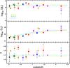 |
Fig. 2 Hα LFs empirical Schechter parameters (using the same colours as Fig. 1) as a function of redshift (at the center redshift of each surveys), along with the evolution of parameters in the models. |
3.1. Model 1
In this model we used a Schechter (1976) parametrization for the luminosity functions and an evolutionary form similar to Geach et al. (2010), 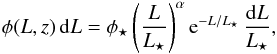 (1)where
-
φ⋆ is the characteristic density of Hα emitters;
-
α is the faint-end slope;
-
L⋆ is the characteristic luminosity at which the Hα luminosity function falls by a factor of e from the extrapolated faint-end power law. It has a value at z = 0 of L⋆,0;
-
and e = 2.718... is the natural logarithm base.
We adopt the same evolutionary form for L⋆ assumed in Geach et al. (2010), and introduce an evolution in φ⋆, 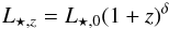 (2)and
  (3)thus φ⋆,0 is the characteristic number density today, which is taken to scale as ∝(1 + z)ϵ at 0 <z<z.break and ∝(1 + z)− ϵ for z>zbreak.
Because the Schechter parameters are correlated, we do not rely on the evolution of the empirical Schechter parameters to constrain their evolution since a unique or fixed α value has not been found or fixed. We instead attempt to reproduce, by mean of a χ2 approach, the observed luminosity functions at different luminosities and redshifts, as described by their Schechter functions in the luminosity range covered by the observations. We, therefore, find the best parameters (reported in Table 2) α = − 1.35, L⋆,0 = 1041.5 erg s-1, φ⋆,0 = 10-2.8 Mpc-3, δ = 2, ϵ = 1, and zbreak = 1.3.
3.2. Model 2
We adopt the same Schechter function for the LFs as for Model 1, but change the evolutionary form for L⋆ as follows:  (4)In this model we normalize the evolution of L⋆ to the maximum redshift available (zbreak = 2.23) and we assume no evolution for φ⋆, i.e. ϵ = 0. Using the same fitting method used for Model 1, to reproduce the observed luminosity functions at different redshift, we find the best fit parameters (reported in Table 2) α = − 1.4, φ⋆,0 = 10-2.7 Mpc-3, c = 0.22, L⋆,zbreak = 1042.59 erg s-1 (ϵ = 0, zbreak = 2.23).
3.3. Model 3
Model 3 is a combined fit to the HiZELS (Sobral et al. 2013), WISP (Colbert et al. 2013), and NICMOS (Yan et al. 1999; Shim et al. 2009) data only. The procedure was designed specifically for use only in the redshift ranges under consideration for the Euclid and WFIRST-AFTA slitless surveys (in particular at 0.7 <z< 2.23). As such, only the three largest compilations in the relevant redshift and flux range were used; in particular the low-z data is not part of the Model 3 fit and we do not display Model 3 results at z< 0.6. We obtained the Model 3 luminosity function parameters and their uncertainties using a Monte Carlo Markov chain (MCMC). In Appendix C, we explore the dependence of the Model 3 fits on the assumptions, fitting methodology, and subsets of the input data used, which is a useful way to assess some types of systematic error.
Model 3 has the advantage of being fit directly to luminosity function data points, and not to the analytic Schechter fit, as done in Model 1 and 2. However, we do not recommend its use at z ≲ 0.6 since it does not incorporate the low-redshift data.
A fit to the data also requires a likelihood function (or error model), in addition to central values for the data points. The luminosity functions provided by individual groups contain the Poisson error contribution, as well as estimated errors from other sources (e.g. uncertainties in the completeness correction). The construction of this model is complicated by two issues: cosmic variance and asymmetric error bars. The model for cosmic variance uncertainties is described in Appendix A. Our default fits are performed using the CV2 model, which allows for a luminosity-dependent bias. The alternative models are CV1, which assumes a luminosity-independent bias, and a no-cosmic variance model. Fitting large numbers of data points can lead to statistically significant biases if the error bars are asymmetric and this is not properly accounted for in the analysis. The treatment of asymmetric error bars is discussed in Appendix B. We use the Poisson option for our primary fits, and consider the other variations in Appendix C.
Fit parameters for the three models considered.
Several models for evolving luminosity functions were investigated and model parameters were fit using the MCMC. All models require a break in the luminosity function to describe the data; the break position L⋆ is taken to be a function of redshift,  (5)Where necessary, we write L⋆,z to denote the characteristic luminosity at redshift z. For the shape of the luminosity function, three forms were considered. The simplest and most commonly used is the Schechter function, but the exponential cutoff is a poor fit to the observations. Two alternative models were considered to fix this: a hybrid model
 ![Mathematical equation: \begin{eqnarray} \phi(L,z) = \frac{\phi_\star}{L_\star} \left( \frac L{L_\star} \right)^\alpha {\rm e}^{-(1-\gamma)L/L_\star} \left[ 1 + (\rme-1)\left(\frac{L}{L_\star}\right)^2 \right]^{-\gamma} ~~~({\rm hybrid}), \label{eq:model1-b.hybrid} \end{eqnarray}](/articles/aa/full_html/2016/06/aa27081-15/aa27081-15-eq148.png) (6)that mixes broken power law and Schechter behaviour; and a broken power law,
(6)that mixes broken power law and Schechter behaviour; and a broken power law, ![Mathematical equation: \begin{eqnarray} \phi(L,z) = \frac{\phi_\star}{L_\star} \left( \frac L{L_\star} \right)^\alpha \left[ 1 + (\rme-1)\left(\frac{L}{L_\star}\right)^\Delta \right]^{-1} ~~~({\rm broken~power~law}). \label{eq:model1-b.broken} \end{eqnarray}](/articles/aa/full_html/2016/06/aa27081-15/aa27081-15-eq149.png) (7)The broken power law is the simplest function1 that interpolates between a faint-end power law φ ∝ Lα and a bright-end power law φ ∝ Lα + Δ. Both of these models are empirically motivated: they were introduced to fit the shallower (than Schechter) cutoff at high L. We also tried an alternative functional form used for low-redshift FIR and Hα data (Saunders et al. 1990, Eq. (1); Gunawardhana et al. 2013, Eq. (11)), however the fit is worse than for the broken power law (χ2 is higher by 8.1, with the same number of degrees of freedom) so we did not adopt it.
(7)The broken power law is the simplest function1 that interpolates between a faint-end power law φ ∝ Lα and a bright-end power law φ ∝ Lα + Δ. Both of these models are empirically motivated: they were introduced to fit the shallower (than Schechter) cutoff at high L. We also tried an alternative functional form used for low-redshift FIR and Hα data (Saunders et al. 1990, Eq. (1); Gunawardhana et al. 2013, Eq. (11)), however the fit is worse than for the broken power law (χ2 is higher by 8.1, with the same number of degrees of freedom) so we did not adopt it.
The Schechter function has one fewer parameter than the others, so in this case φ⋆ was allowed to have an exponential evolution with scale factor a = 1/(1 + z),  (8)with (d/da)log 10φ⋆ taken to be a constant. The broken power law model was used for the reference fit, since it gives the best χ2.
These models have Npar = 6 parameters, 3 parameters besides the standard Schechter parameters (φ⋆, α, L⋆), whose meaning, is as follows:
-
(d/da)log 10φ⋆ (for the Schechter function) characterizes density evolution; it is positive if Hα emitters get more abundant at late times.
-
γ (hybrid model only) interpolates between an exponential or Schechter-like cutoff at high L (γ = 0) or a broken power law form (γ = 1: the power law index changes by 2 between the faint and bright ends). Values of γ> 1 are not allowed.
-
Δ (broken power law model only) is the difference between bright and faint-end slopes.
-
L⋆,z has a high-z extrapolated limiting value2 (L⋆,∞) and a value at z = 0.5 (L⋆,0.5). The sharpness of the fall-off in L⋆ at low redshift is controlled by β. In some models, log 10L⋆,2.0 (the value at z = 2.0) was used instead of log 10L⋆,∞ to reduce the degeneracy with β.
The three models differ most strongly in their assumed form at the high-luminosity end: the broken power law has a power law scaling (with slope α − Δ), whereas the Schechter function has an exponential cutoff. The hybrid model has an exponential cutoff if γ< 1, but its steepness is decoupled from L⋆ – as γ → 1, the scale luminosity in the cutoff L⋆/ (1 − γ) can be much greater than the luminosity at the break L⋆.
The likelihood evaluation predicts the luminosity function averaged over a bin of log 10LHα and enclosed volume [ D(z) ] 3 using NG × NG Gauss-Legendre quadrature scheme (for slitless surveys) or an NG-point Gaussian quadrature (for narrow-band surveys, where there is no need to do a redshift average). The fiducial value of the quadrature parameter is NG = 3. A flat prior was used on the 5 or 6 parameters (α,log 10φ⋆,log 10L⋆,2.0,log 10L⋆,0.5,β and γ or Δ, as appropriate). Chains are run with a Metropolis-Hastings algorithm; at the end a minimizing algorithm is run on the χ2 to find the maximum likelihood model.
The best fit model (lowest χ2) is the broken power law model with parameters (reported in Table 2) α = − 1.587, Δ = 2.288, log 10φ⋆,0 = − 2.920, log 10L⋆,2.0 = 42.557, log 10L⋆,0.5 = 41.733, and β = 1.615 (and the corresponding log 10L⋆,∞ = 42.956). The faint-end slope of α = − 1.587 is 2.0σ shallower than the ultraviolet LF slope of −1.84 ± 0.11 measured by Reddy et al. (2008), and 1.5σ shallower than −1.73 ± 0.07 measured by Reddy & Steidel (2009) at z ≈ 2. The residuals from this fit are shown in Fig. 3.
 |
Fig. 3 Residuals to the Hα luminosity function fits for Model 3, plotted as a function of observed-frame Hα flux at the bin centre (horizontal axis). All redshifts are plotted together. The green lines show the fit line and factors of 2 above and below. The error bars shown do not include the cosmic variance, which is included in the fit but is highly correlated across luminosity bins. |
4. Comparison to observed luminosity functions
The three empirical models constructed are plotted in Fig. 1 in different redshift bins, and compared to the observed HαLFs. The Schechter parameters for data and models are also shown, only for illustrative purpose, in Fig. 2. Note, however, that, since the parameters are correlated, a direct comparison between them is not straightforward, in particular Model 3 assumes also a different form for the LFs.
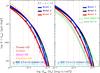 |
Fig. 4 Left panel: cumulative Hα number counts, integrated over the redshift ranges 0.7 <z< 1.5 (WISP range). The observed counts from the WISP survey (Colbert et al. 2013) are shown (blue circles) and from new WISP analysis by Mehta et al. (2015; cyan circles), and compared to the empirical Model 1, 2, and 3, (blue, black and red lines, respectively). Also shown (as dotted lines and empty squares) are the counts obtained integrating the observed LFs (see legend) in the same redshift range. Right panel: same cumulative Hα number counts compared to the predictions from L12 mocks (green dashed and solid lines using intrinsic and extincted Hα fluxes, respectively) and GP14 mocks (dark and light grey for H< 27 and H< 24 mocks, respectively). |
Given the large scatter in the observed LFs covering similar redshift ranges, all the 3 models provide a reasonable description of the data. Indeed, while it is difficult to choose a best model, among the three, overall they describe well the uncertainties and the scatter between different observed LFs, in particular at high-z.
Comparing different redshift bins, it is evident that at low-z the models evolve rapidly in luminosity, as clearly visible also in the evolution of L⋆ parameter, resulting in an increase of the density of high luminosity Hα emitters. Since at high-z, instead, all 3 models evolve mildly in luminosity and density, or even slightly decrease in density (for Model 1), as a consequence the density of high-L objects is almost constant.
Finally, we note that the main difference between the 3 models at all redshifts is at the bright-end of the luminosity function. Model 1 has the lower high-luminosity end, but is similar in shape to Model 2, (both assuming a Schechter form), while Model 3 has the most extended bright-end, while it is slightly lower at intermediate luminosities, and has the steepest faint-end slope. This occurs because of the different functional form used in Model 3. Current uncertainties in the bright-end of the empirical HαLFs, do not allow strong constraint on the functional form. Actually, recent analysis of GAMA and SDSS surveys (Gunawardhana et al. 2013, 2015) and of WISP (Mehta et al. 2015) suggest a LF more extended than a Schechter function but only at very bright luminosity (>1043 erg/s). Further analysis on wider area will provide new insight on this issue.
5. Number counts and redshift distribution of Hα emitters
The cumulative counts, as a function of Hα flux limit, predicted by the models are shown in Fig. 4. We derive the cumulative counts in the same redshift range covered by the WISP slitless data, i.e. 0.7 <z< 1.5. For comparison we show the observed Hα WISP counts, taken from Table 2 of Colbert et al. (2013) and corrected for [N ii] emission as indicated in the original paper, with LHα = 0.71(LHα + L[ N ii ]), for consistency with the WISP Hα LF used here. Besides WISP counts, we show also the predicted counts using single luminosity functions at different redshifts (integrated over the same redshift range 0.7 <z< 1.5). The three models reproduce well the scatter between the observed counts and observed luminosity functions, with Model 3 giving the lowest counts due to the large weight assigned to the (lower amplitude) HiZELS and WISP samples.
Redshift distributions for a range of limiting fluxes (in units of 10-16 erg cm-2 s-1) from the 3 empirical Models (1, 2, 3).
At the depth and redshift range of the originally planned Euclid Wide grism survey (Laureijs et al. 2011), i.e. FHα> 3 × 10-16 erg cm-2 s-1, and 1.1 <λ< 2.0 μm (sampling Hα at 0.70 <z< 2.0), Models 1, 2, and 3 predict about 2490, 3370, and 1220 Hα emitters per deg2, respectively. This increases to 42 500, 39 700, and 28 100 Hα emitters per deg2 for FHα> 5 × 10-17 erg cm-2 s-1 as originally planned for the Deep Euclid specroscopic survey (see Table 3).
The WFIRST-AFTA mission will have less sky coverage than Euclid (2200 deg2 instead of 15 000 deg2), but with its larger telescope will probe to fainter fluxes. Its grism spans the range from 1.35–1.89 μm.3 The single line flux limit4 varies with wavelength and galaxy size; at the center of the wave band for a point source, and for a pre-PSF effective radius of 0.2 arcsec (exponential profile), it is 9.5 × 10⁻¹⁷ erg cm-2 s-1. The three luminosity functions integrated over the WFIRST-AFTA sensitivity curve5 predict an available galaxy density of 11 900, 12 400, and 7200 gal deg-2 (for Models 1, 2, and 3 respectively), in the redshift range 1.06 <z< 1.88.
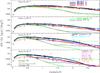 |
Fig. 5 Hα redshift distribution above various flux thresholds (from 0.5 × 10⁻¹⁶ erg cm-2 s-1 to 3 × 10-16 erg cm-2 s-1, from top to bottom panels). Observed redshift distributions are indicated with open circles, while data obtained integrating LFs are shown with squares. HaLF predictions from Model 1, 2, 3 are shown as thick solid lines. The predictions from L12 mocks (green dashed and solid lines using intrinsic and extincted Hα fluxes, respectively) and GP14 mocks (dark and light grey for H< 27 and H< 24 mocks, respectively) are also shown. |
The previous community standard luminosity function model, used for the 2011 Euclid Red Book (Laureijs et al. 2011) and in pre-2012 WFIRST studies (Green et al. 2011), is that of Geach et al. (2010) divided by a factor of 1.257. This luminosity function predicts 7470 and 41 500 Hα emitters per deg2 in the same redshift range (0.7 <z< 2) and flux limits (>3 or 0.5 × 10⁻¹⁶ erg cm-2 s-1) of the original wide and deep Euclid surveys. This is a factor of about 2–6 more than estimated here at bright fluxes and a similar number at faint fluxes. The difference is partly due to the factor of ln10 ≈ 2.3 from the convention for φ⋆ in the Geach et al. (2008) luminosity function, and partly because Geach et al. (2010) used the brightest and highest LF by Yan et al. (1999) as the principal constraint in the z ~ 1.3 range; in contrast later WISP and HiZELS samples have found fewer bright Hα emitters at this redshift.
Very recently, from the new analysis by Mehta et al. (2015) of the bivariate Hα-[OIII] luminosity function for the WISP survey, over roughly double the area used by Colbert et al. (2013), they expect in the range 0.7 <z< 2 about 3000 galaxies/deg2 for the nominal flux limit of Euclid (>3 × 10-16 erg cm-2 s-1) and ~20 000 galaxies/deg2 for a fainter flux limit (>1 × 10-16 erg cm-2 s-1, the baseline depth of WFIRST-AFTA). We note that these expectations are more consistent with our two higher models, i.e. Model 1 and 2, than with our lowest Model 3. Fig. 4 shows their counts at 0.7 <z< 1.5 (from their Table 4).
The redshift distributions (dN/ dz) at various Hα flux limits (0.5,1,2,3 × 10-16 erg cm-2 s-1) relevant to the Euclid and WFIRST-AFTA surveys are shown in Fig. 5. Besides the observed WISP cumulative counts (from their Table 2, interpolating at the Hα flux limits corrected for [N ii] contamination), we show also dN/ dz derived using single luminosity functions observed at different redshifts (integrated over the observed redshift range and plotted at the central redshift of each survey). It is evident that the current scatter in the observed luminosity function at z> 1, introduces a large uncertainty in the predictions, in particular at bright fluxes. The differences between our three models are due to the different evolution and parametrization assumed for the luminosity functions. In particular, as discussed in previous section, with Model 2 having a brighter L⋆ at high redshifts, the predicted dN/ dz is higher at bright fluxes at z> 1.2. Clearly, this is a regime where large areas data are almost not available, and Euclid will cover this gap. At faint fluxes, instead Model 1 and 2 are more similar, sampling the low luminosity end of their similar LFs, with Model 1 having a slightly steeper LF and higher φ⋆. Model 3 predicts a density of emitters that is a factor from 1.5 to 2.5 lower than the other models from the faint to the bright fluxes considered, at all redshifts.
The new analysis by Mehta et al. (2015) of the WISP survey is also shown in Fig. 5. The number densities at z ~ 2 have been derived using the [OIII] line luminosity function, and assuming that the relation between Hα and [OIII] luminosity does not change significantly over the redshift range. The expectations are quite high but consistent within the error-bars with our highest model.
In Table 3 we list the predicted redshift distributions in redshift bins of width of Δz = 0.1, at various limiting fluxes, for the three different models6. In addition we list also the expected numbers for the 3 models at different flux limits and in the typical redshift ranges for future NIR space missions. In particular for the original Euclid wide/deep surveys, designed to cover in Hα the redshift range 0.7 <z< 2.0 at flux limit about 3/0.5 × 10-16 erg cm-2 s-1, using two grisms (blue+red), we expect about 1200/28 000–3400/40 000 objects for deg2. We note that for the wide survey similar number densities can be reached using the same exposure time but a single grism, for example covering the redshift range 0.9 <z< 1.8 to a flux limit of 2 × 10-16 erg cm-2 s-1, we expect about 2000–4800 Hα emitters/deg2, therefore in total 30–72 million of sources will be mapped by Euclid. For the Euclid deep survey an extension of the grism to bluer wavelenghts, i.e. to lower redshift, for example 0.4 <z< 1.8, will increase the number densities to about 32 000–48 000 deg-2 and therefore 1.3–2 million of emitters mapped in 40 deg2.
We remind the reader that these predictions are in terms of observed Hα flux, i.e. include intrinsic dust extinction in the Hα emitters, and is corrected for [N ii] contamination. However, at the nominal resolution of both Euclid and WFIRST-AFTA, these lines will be partially blended; thus, here we may be underestimating the final detection significance of the galaxies, i.e. the sensitivity to Hα flux is better than the single line sensitivity described here, even if not by the full factor of the Hα:(Hα+[N ii]) ratio. For this reason, we expect that our analysis is somewhat conservative.
Finally, future NIR space mission will use slitless spectroscopy and therefore suffer from some degree of contamination in the spectra (depending on the rotation angles used), as well as misidentification of different emission lines, which will decrease the effective numbers of emitters available for science. We note, however, that unlike the WISP survey, both Euclid and WFIRST will use multiple dispersion angles to break the degeneracy in which lines from different sources at different wavelengths can fall on the same pixel. Therefore the number of objects computed from the HαLF should be reduced by the completeness factor before being used in cosmological forecasts. Preliminary estimates of this factor have been included in the Euclid (Laureijs et al. 2011) and WFIRST-AFTA (Spergel et al. 2015b) forecasts, and the estimates of completeness will continue to be refined as the instrument, pipeline, and simulations are developed. The problem of sample contamination depends on the abundance of other line emitters (i.e. not Hα), and the data available to reject them – photometric redshifts and secondary lines. The rejection logic is specific to each survey as it depends on wavelength range, grism resolution (e.g. both Euclid and WFIRST-AFTA would separate the [O iii] doublet), and which deep imaging filters are available. Pullen et al. (2016) present an example for WFIRST-AFTA (combined with LSST photometry) that should achieve a low contamination rate, albeit under idealized assumptions. It is presumed that deep spectroscopic training samples will be required to characterize the contamination rate in the cosmology sample. The redshift completeness factor could also be density dependent, and its estimation will require mock catalogues with clustering. The models presented here, therefore, will provide a key input to instrument simulations that aim to forecast the completeness of the Euclid and WFIRST-AFTA spectroscopic samples.
6. Comparison to semi-analytic mock catalogs
We compare our empirical Hα models to Hα number counts and redshift distributions from mock galaxy catalogues built with the semi-analytic galaxy formation model GALFORM (e.g. Cole et al. 2000; Bower et al. 2006). The dark matter halo merger trees with which GALFORM builds a galaxy catalogue are extracted from two flat ΛCDM simulations of 500 Mpc/h aside, differing only by their cosmology: (i) the Millennium simulation (Springel et al. 2005) with Ωm = 0.25, h = 0.73 and σ8 = 0.90; (ii) the MR7 simulation (Guo et al. 2013) with Ωm = 0.272, h = 0.704 and σ8 = 0.81. Merson et al. (2013) provides a method for constructing lightcone galaxy catalogues from the GALFORM populated simulation snapshots, onto which observational selections can be applied, like an apparent H-band magnitude limit. These lightcones come with an extensive list of galaxy properties, including the observed and cosmological redshifts, the observed magnitudes and rest-frame absolute magnitudes in several bands, and the observed fluxes and rest-frame luminosities of several emission lines. For the present work, we have analysed lightcones built with the Lagos et al. (2012) GALFORM model7 (L12 mocks, hereafter) and with the Gonzalez-Perez et al. (2014) GALFORM model8 (GP14 mocks hereafter), using respectively the Millennium and MR7 simulations. It is essential to point out that the model parameters for Lagos et al. (2012) and Gonzalez-Perez et al. (2014) are calibrated using mostly local datasets, such as the optical and NIR galaxy luminosity functions. In particular, no observational constraints from emission line galaxies are used in the calibration process.
We are most interested in the H band magnitude and the Hα flux. To assign galaxy properties, the stellar population synthesis models from Bruzual & Charlot (2003; GISSEL 99 version) is used with the Kennicutt (1983) initial mass function over the range 0.15 M⊙<m< 120 M⊙. To calculate the Hα flux, the number of Lyman continuum photons is computed from the star formation history predicted for the galaxy. The Stasińska (1990) models is used to obtain the line luminosity from the number of continuum photons (T = 45 000 K, n = 10 and Ns = 1), testing that the choice of the HII region properties from the Stasinska models does not have an impact on the number of Hα emitters. The dust extinction law is the one for the Milky Way by Ferrara et al. (1999). Broad-band magnitudes are reported on the AB scale.
In this work, we have analysed the lightcones constructed to emulate the Euclid surveys. In particular, in order to explore the effect of the selection on the density of Hα emitters, we have explored deep mocks selected in magnitude provided on different areas (100 deg2 limited to H< 27 for L12 mocks and 20 deg2 limited to H< 27 or FHα> 3 × 10-18 erg cm-2 for GP14 one).
In Fig. 4 we show the cumulative number densities derived using different mock catalogues in the redshift range 0.7 <z< 1.5. The two lightcones, irrespective of the GALFORM version used, underpredict the cumulative counts at all Hα fluxes explored (from >10-15 up to >10-17 erg cm-2 s-1), i.e. they are therefore in disagreement with the observed counts from WISP survey and with most of the counts derived from empirical LF, with the only exception of HiZELS Sobral et al. (2013). We have also tested the effect of limiting magnitudes on the Hα counts from the GP14 mock, finding that a mock selected to H< 24 underestimates the density of Hα emitters but only at very faint fluxes (3 × 10-17 erg cm-2 s-1).
Finally, we compare the mocks with our empirical models. We find that the mocks predict counts, in the redshift 0.7 <z< 1.5, lower than our models; for example the GP14 mock is lower than Model 1 by a factor 2 to 4.5 from faint to bright flux limits. The L12 mock predictions are even slightly lower than the GP14 mock.
We have also explored the effect of dust extinction, showing the cumulative counts for intrinsic Hα fluxes (i.e. before dust extinction applied) for the L12 mock in Fig. 4. In this case the simulated mock predicts very high number densities at bright fluxes (>10-15 erg cm-2 s-1), above all the data available, but agree with the two faintest data from the WISP survey, which are close to the deep Euclid flux limit. We note that the effect of dust extinction is flux dependent in the L12 mock. However, also predictions using intrinsic Hα fluxes and applying a dust extinction of 1 mag. (0.4 dex), as usually applied reversally in the data, provide counts even lower than mocks shown and flatter than our 3 models and explored data.
In Fig. 5 we further analyse the predictions for the redshift distribution, at various flux limits, from the lightcones. It is evident that redshift distribution from mocks, irrespective of the explored flux limits, are consistent with data at low redshift, while they are systematically lower than data at z> 1, despite the large dispersion in the data. The number densities from GP14 mock are lower than our models and data by a factor up to 10 at faint fluxes and z> 1.5. The L12 mock predictions are even lower than the GP14 ones, in particular at z> 1.5, where at all fluxes except for faint ones, the number densities continue to decrease with z and not present a flattening as in the GP14 mock. At low redshift, instead, the mocks cover relatively well the range of number densities predicted by our models, being more similar to Model 1, 2 at z< 0.7.
In addition, we have explored the effect of a brighter H-band magnitude limit (H< 24 compared to the original H< 27) in the GP14 mock, finding that it does not affect strongly the redshift distribution at all flux explored, but fainter one at high redshift (z> 2). Finally, we note that only using intrinsic Hα fluxes, i.e. before dust extinction has been applied, the L12 mock predicts a tail in the redshift distribution at high redshift (z> 1.5 − 2) and bright flux limits consistent with our empirical models or even higher at z> 2 (note however that empirical models and data are not corrected for dust extinction).
We remind the reader that the SAMs used here are not calibrated using emission line datasets. The predictions of mocks for the HαLFs have been analysed by Lagos et al. (2014, see their Fig. 1). In a future work (Shi et al., in prep.), we will analyse in detail an optimization of the mocks to reproduce empirical HαLFs, taking into account also the contribution of AGN, which might affect this comparison.
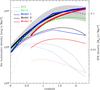 |
Fig. 6 Hα luminosity density of the Universe as a function of redshift. The solid thick lines show the total luminosity density, whereas the thin solid curves show the luminosity density for emitters at F> 10-16 erg cm-2 s-1 (upper set of curves) and F> 3 × 10-16 erg cm-2 s-1 (lower set of curves). The different colours are codes for each model (blue, Model 1; black, Model 2; and red, Model 3). Also shown is the calculation of total Hα luminosity density based on the star formation histories of Madau & Dickinson (2014, green dashed) and Behroozi et al. (2013, gray dashed and shaded area). On the right axis we report also the SFR density scale for a Chabrier IMF. |
7. Hα luminosity density and star formation history
Finally, we consider the implications of our empirical models for the global Hα luminosity density of the Universe, and the closely related cosmic star formation history.
The Hα luminosity density is shown in Fig. 6, as predicted by each model. We show the total (integrating the functional form over all luminosities), along with the predictions by each model imposing flux limits at F> 10-16 erg cm-2 s-1 and F> 3 × 10-16 erg cm-2 s-1. Note the excellent agreement for the integrated luminosity functions, even though the bright end is quite different for the 3 models (being lower for Model 3). As one can see from the dashed curves, the depth probed by BAO surveys picks up only a portion of the overall Hα emission in the Universe: for example, Models 1, 2, and 3 predict that 31, 39, and 23 per cent respectively of the Hα emission passes the flux cut F> 10-16 erg cm-2 s-1 at z = 1.5. At z = 1.5, to represent half of the overall Hα emission, we would need to lower the flux cut to (3.1 − 6.6) × 10-17 erg cm-2 s-1.
Also shown in Fig. 6 is the observed (i.e. no corrected for extinction) Hα luminosity density derived from the star formation history by Madau & Dickinson (2014) and Behroozi et al. (2013) along with its dispersion. We, respectively, use the conversion of LHα/SFR = 7.9 × 10-42 erg s-1 yr (Kennicutt 1998), appropriate for a Salpeter (1955) initial mass function used by Madau & Dickinson (2014), and adding a factor of 1.7 boost, appropriate for the Chabrier (2003) initial mass function, used by Behroozi et al. (2013). For consistency, the same receipt used to correct for dust extinction in Hα surveys to derive the above SFHs, has been used to correct them back, i.e. the derived Hα luminosity density has been reduced by a factor of 100.4 in accordance with the commonly-assumed 1 mag of extinction (Hopkins et al. 2004). This procedure is not an independent check, since Behroozi et al. (2013) refer to some of the same data used in this paper, but does provide an assessment of the overall consistency of the literature, particularly given that Madau & Dickinson (2014) and Behroozi et al. (2013) consider many other tracers of star formation (i.e. not just Hα) as well. The agreement is within a factor of 2 difference at z ~ 2 for one of the star formation histories, and better for other cases – we consider this good, given the uncertainties in the extrapolation to fluxes lower than that covered by Hα surveys. We further note that the agreement is still recovered if we consider a more sophisticated treatment of the dust extinction, varying it with redshift as derived from the ratio between FUV and FIR luminosity densities (Burgarella et al. 2013). However, this procedure introduces additional and uncertain assumptions on the dust extinction law and on the ratio between the extinction in the continuum and in the emission lines (Calzetti et al. 2000).
Finally, we note that on the contrary the SAMs considered in this paper predict a star formation density below the values deduced from the observations at 0.3 <z< 2 (see Lagos et al. 2014, Fig. 3). We emphasize here that the observed/exctincted Hα luminosity density is inferred after applying a correction for dust extinction and after extrapolation down to faint unobserved Hα luminosities, introducing therefore further uncertainties in the comparison with models.
8. Summary
The Hα luminosity function is a key ingredient for forecasts for future dark energy surveys, especially at z ≳ 1 where blind emission-line selection is one of the most efficient ways to build large statistical samples of galaxies with known redshifts. We have collected the main observational results from the literature and provided three empirical Hα luminosity function models. Models 1 and 2 have the advantage of combining the largest amount of data over the widest redshift range, whereas Model 3 focuses only on fitting the range of redshift and flux most relevant to Euclid and WFIRST-AFTA, but covered by more sparse and uncertain data.
The three model Hα luminosity functions are qualitatively similar, but there are differences of up to a factor of 3 (ratio of highest to lowest) in the most discrepant parts of Table 3. This is despite the small aggregate statistical errors (for example ±17 per cent at 2σ for Model 3 in the redshift range of 0.9 <z< 1.8 and FHα> 2 × 10-16 erg cm-2 s-1). Some of this is due to real differences in the input datasets. In particular, our investigations of the input data in Model 3 show that minor details in the fits (such as the treatment of asymmetric error bars and the finite width of luminosity and redshift bins) as well as cosmic variance affect the outcome by more than the statistical errors in the fits. All of these models predict significantly fewer Hα emitters than were anticipated several years ago. However, even according to our most conservative model, the upcoming space missions Euclid and WFIRST-AFTA will chart the three-dimensional positions of tens of millions of galaxies at z ≳ 0.9, a spectacular advance over the capabilities of present-day redshift surveys. For instance, covering the redshift range 0.9 <z< 1.8 to a flux limit of 2 × 10-16 erg cm-2 s-1, we expect about 2000–4800 Hα emitters/deg2, therefore in total 30–72 million of sources will be mapped over 15 000 deg2 by the Euclid wide survey and 1.3-2 million of emitters will be mapped in 40 deg2 by the Euclid deep survey in the range 0.4 <z< 1.8 at fluxes above 0.5 × 10⁻¹⁶ erg cm-2 s-1. At the WFIRST-AFTA sensitivity, we predict in the redshift range 1 <z< 1.9 about 16 to 26 million of galaxies at fluxes above ~1 × 10-16 erg cm-2 s-1 over 2200 deg2. The models presented here also provide a key input for the scientific optimization of the survey parameters of these missions and for cosmological forecasts from the spectroscopic samples of Euclid and WFIRST-AFTA. The HαLFs derived here must be folded through instrument performance, observing strategy and completeness, and modelling of the galaxy power spectrum in order to arrive at predicted BAO constraints. The previous Euclid forecasts (Amendola et al. 2013) are currently being updated with the new HαLFs and updated instrument parameters, and we anticipate that the public documents will be updated soon. The HαLFs presented here have already been incorporated in the most recent WFIRST-AFTA science report (Spergel et al. 2015b).
The factor of e − 1 = 1.718... in Eq. (7) does not lead to any physical change in the model – it is equivalent to a re-scaling of the break luminosity L⋆. With the stated normalization, L⋆ is the luminosity at which the LF falls to 1/e of the faint-end power law, which is the same meaning that it has in the Schechter function; without this factor, L⋆ would correspond to the luminosity at which the LF falls to 1/2 of the faint-end power law.
Of course, at very high redshift the HαLF must fall off since there are no galaxies. We remind the reader that the empirical models built here may not be valid outside the range of redshifts spanned by the input data.
The grism red limit was 1.95 μm in the original WFIRST-AFTA design; it was changed to 1.89 μm in fall 2014 due to an increase in the baseline telescope operating temperature.
The Hα+[N ii] complex is partially blended at WFIRST-AFTA resolution; the exposure time calculator (Hirata et al. 2012) now contains a correction for this effect.
Spergel et al. (in prep.). We also used the j = 2 galaxy size distribution in the WFIRST exposure time calculator (Hirata et al. 2012).
Complete tables for the 3 models at limiting fluxes from 0.1 to 100 × 10-16 erg cm-2 s-1 are available at http://www.bo.astro.it/~pozzetti/Halpha/Halpha.html
Lagos et al. (2012)Euclid lightcones are available from http://community.dur.ac.uk/a.i.merson/lightcones.html
Gonzalez-Perez et al. (2014) lightcones are available from the Millennium Database, accessible from http://www.icc.dur.ac.uk/data/
There are redshift-space distortion terms in Eq. (A.4) that we have neglected; we do not believe the fidelity of the model warrants a more intricate correction.
Technically, one with large second derivative.
For this fit, the Hα luminosities were re-scaled, and the differential luminosity function was appropriately transformed using the Jacobian of the uncorrected-to-corrected flux transformation.
The correction in Eq. (C.1) is an overestimate in cases where Hα falls in the narrow bandpass and one or both of the [N ii] lines do not. It is an underestimate if [N ii] 6583 Å falls in the narrow band and Hα does not, but since Hα is almost always stronger this is not as much of an issue at the top of the luminosity function.
Acknowledgments
We wish to thank James Colbert, David Sobral, Lin Yan, Gunawardhana Madusha and Ly Chun for their help with the input luminosity function data for this paper. We thank Bianca Garilli, Gigi Guzzo, Yun Wang, Will Percival, Claudia Scarlata and Gianni Zamorani to stimulate this work and for useful discussions and comments. L.P. and A.C. acknowledge financial contributions by grants ASI/INAF I/023/12/0 and PRIN MIUR 2010-2011 “The dark Universe and the cosmic evolution of baryons: from current surveys to Euclid.” C.H. has been supported by the United States Department of Energy under contract DE-FG03-02-ER40701, the David and Lucile Packard Foundation, the Simons Foundation, and the Alfred P. Sloan Foundation. This work was supported by the STFC through grant number ST/K003305/1. J.E.G. thanks the Royal Society. P.N. acknowledges the support of the Royal Society through the award of a University Research Fellowship and the European Research Council, through receipt of a Starting Grant (DEGAS-259586). C.M.B., P.N. and S.D. acknowledge the support of the Science and Technology Facilities Council (ST/L00075X/1). The simulations results used the DiRAC Data Centric system at Durham University and funded by BIS National E-infrastructure capital grant ST/K00042X/1, STFC capital grants ST/H008519/1 and ST/K00087X/1, STFC DiRAC Operations grant ST/K003267/1 and Durham University.
References
- Albrecht, A., Bernstein, G., Cahn, R., et al. 2006, ArXiv e-prints [arXiv:astro-ph/0609591] [Google Scholar]
- Amendola, L. et al. 2013, Liv. Rev. Rel., 16, 6 [Google Scholar]
- Anderson, L., Aubourg, É., Bailey, S., et al. 2014, MNRAS, 441, 24 [NASA ADS] [CrossRef] [Google Scholar]
- Behroozi, P. S., Wechsler, R. H., & Conroy, C. 2013, ApJ, 770, 57 [NASA ADS] [CrossRef] [Google Scholar]
- Blake, C., Davis, T., Poole, G. B., et al. 2011a, MNRAS, 415, 2892 [NASA ADS] [CrossRef] [Google Scholar]
- Blake, C., Kazin, E. A., Beutler, F., et al. 2011b, MNRAS, 418, 1707 [NASA ADS] [CrossRef] [MathSciNet] [Google Scholar]
- Bond, J. R., Jaffe, A. H., & Knox, L. 1998, Phys. Rev. D, 57, 2117 [NASA ADS] [CrossRef] [Google Scholar]
- Bond, J. R., Jaffe, A. H., & Knox, L. 2000, ApJ, 533, 19 [NASA ADS] [CrossRef] [Google Scholar]
- Bruzual, G., & Charlot, S. 2003, MNRAS, 344, 1000 [NASA ADS] [CrossRef] [Google Scholar]
- Burgarella, D., Buat, V., Gruppioni, C., et al. 2013, A&A, 554, A70 [NASA ADS] [CrossRef] [EDP Sciences] [Google Scholar]
- Calzetti, D., Armus, L., Bohlin, R. C., et al. 2000, ApJ, 533, 682 [NASA ADS] [CrossRef] [Google Scholar]
- Chabrier, G. 2003, PASP, 115, 763 [NASA ADS] [CrossRef] [Google Scholar]
- Colbert, J. W., Teplitz, H., Atek, H., et al. 2013, ApJ, 779, 34 [NASA ADS] [CrossRef] [Google Scholar]
- Cole, S., Percival, W. J., Peacock, J. A., et al. 2005, MNRAS, 362, 505 [NASA ADS] [CrossRef] [Google Scholar]
- Eisenstein, D. J., Zehavi, I., Hogg, D. W., et al. 2005, ApJ, 633, 560 [NASA ADS] [CrossRef] [Google Scholar]
- Ferrara, A., Bianchi, S., Cimatti, A., & Giovanardi, C. 1999, ApJS, 123, 437 [NASA ADS] [CrossRef] [Google Scholar]
- Gallego, J., Zamorano, J., Aragon-Salamanca, A., & Rego, M. 1995, ApJ, 455, L1 [NASA ADS] [CrossRef] [Google Scholar]
- Geach, J. E., Smail, I., Best, P. N., et al. 2008, MNRAS, 388, 1473 [NASA ADS] [CrossRef] [Google Scholar]
- Geach, J. E., Cimatti, A., Percival, W., et al. 2010, MNRAS, 402, 1330 [NASA ADS] [CrossRef] [Google Scholar]
- Geach, J. E., Sobral, D., Hickox, R. C., et al. 2012, MNRAS, 426, 679 [NASA ADS] [CrossRef] [Google Scholar]
- Glazebrook, K., Baldry, I., Moos, W., Kruk, J., & McCandliss, S. 2005, New Astron. Rev., 49, 374 [NASA ADS] [CrossRef] [Google Scholar]
- Green, J., Schechter, P., Baltay, C., et al. 2011, ArXiv e-prints [arXiv:1108.1374] [Google Scholar]
- Green, J., Schechter, P., Baltay, C., et al. 2012, ArXiv e-prints [arXiv:1208.4012] [Google Scholar]
- Gonzalez-Perez, V., Lacey, C. G., Baugh, C. M., et al. 2014, MNRAS, 439, 264 [NASA ADS] [CrossRef] [Google Scholar]
- Gunawardhana, M. L. P., Hopkins, A. M., Bland-Hawthorn, J., et al. 2013, MNRAS, 433, 2764 [NASA ADS] [CrossRef] [Google Scholar]
- Gunawardhana, M. L. P., Hopkins, A. M., Taylor, E. N., et al. 2015, MNRAS, 447, 875 [NASA ADS] [CrossRef] [Google Scholar]
- Guo, Q., White, S., Angulo, R., et al. 2013, MNRAS, 428, 1351 [NASA ADS] [CrossRef] [Google Scholar]
- Guzzo, L., Pierleoni, M., Meneux, B., et al. 2008, Nature, 451, 541 [NASA ADS] [CrossRef] [PubMed] [Google Scholar]
- Hayes, M., Schaerer, D., & Östlin, G. 2010, A&A, 509, L5 [NASA ADS] [CrossRef] [EDP Sciences] [Google Scholar]
- Hirata, C. M., Gehrels, N., Kneib, J.-P., et al. 2012, ArXiv e-prints [arXiv:1204.5151] [Google Scholar]
- Hopkins, A. M. 2004, ApJ, 615, 209 [NASA ADS] [CrossRef] [Google Scholar]
- Hopkins, A. M., Connolly, A. J., & Szalay, A. S. 2000, AJ, 120, 2843 [NASA ADS] [CrossRef] [Google Scholar]
- Kaiser, N. 1987, MNRAS, 227, 1 [NASA ADS] [CrossRef] [Google Scholar]
- Kazin, E. A., Sánchez, A. G., Cuesta, A. J., et al. 2013, MNRAS, 435, 64 [NASA ADS] [CrossRef] [Google Scholar]
- Kazin, E. A., Koda, J., Blake, C., et al. 2014, MNRAS, 441, 3524 [NASA ADS] [CrossRef] [Google Scholar]
- Kennicutt, Jr., R. C. 1983, ApJ, 272, 54 [NASA ADS] [CrossRef] [EDP Sciences] [Google Scholar]
- Kennicutt, Jr., R. C. 1998, ARA&A, 36, 189 [Google Scholar]
- Lagos, C. d. P., Bayet, E., Baugh, C. M., et al. 2012, MNRAS, 426, 2142 [NASA ADS] [CrossRef] [Google Scholar]
- Lagos, C. d. P., Baugh, C. M., Zwaan, M. A., et al. 2014, MNRAS, 440, 920 [NASA ADS] [CrossRef] [Google Scholar]
- Laureijs, R., Amiaux, J., Arduini, S., et al. 2011, ArXiv e-prints [arXiv:1110.3193] [Google Scholar]
- Lee, J. C., Ly, C., Spitler, L., et al. 2012, PASP, 124, 782 [NASA ADS] [CrossRef] [Google Scholar]
- Ly, C., Malkan, M. A., Kashikawa, N., et al. 2007, ApJ, 657, 738 [NASA ADS] [CrossRef] [Google Scholar]
- Ly, C., Lee, J. C., Dale, D. A., et al. 2011, ApJ, 726, 109 [NASA ADS] [CrossRef] [Google Scholar]
- Madau, P., & Dickinson, M. 2014, ARA&A, 52, 415 [NASA ADS] [CrossRef] [Google Scholar]
- Mehta, V., Scarlata, C., Colbert, J. W., et al. 2015, ApJ, 811, 141 [NASA ADS] [CrossRef] [Google Scholar]
- Merson, A. I., Baugh, C. M., Helly, J. C., et al. 2013, MNRAS, 429, 556 [NASA ADS] [CrossRef] [Google Scholar]
- Orsi, A., Baugh, C. M., Lacey, C. G., et al. 2010, MNRAS, 405, 1006 [NASA ADS] [Google Scholar]
- Padmanabhan, N., Xu, X., Eisenstein, D. J., et al. 2012, MNRAS, 427, 2132 [NASA ADS] [CrossRef] [MathSciNet] [Google Scholar]
- Percival, W. J., Cole, S., Eisenstein, D. J., et al. 2007, MNRAS, 381, 1053 [NASA ADS] [CrossRef] [MathSciNet] [Google Scholar]
- Percival, W. J., Reid, B. A., Eisenstein, D. J., et al. 2010, MNRAS, 401, 2148 [NASA ADS] [CrossRef] [Google Scholar]
- Perlmutter, S., Aldering, G., Goldhaber, G., et al. 1999, ApJ, 517, 565 [NASA ADS] [CrossRef] [Google Scholar]
- Pullen, A., Hirata, C., Doré, O., & Raccanelli, A. 2016, PASJ, 68, 12 [NASA ADS] [CrossRef] [Google Scholar]
- Reddy, N. A., & Steidel, C. C. 2009, ApJ, 692, 778 [NASA ADS] [CrossRef] [Google Scholar]
- Reddy, N. A., Steidel, C. C., Pettini, M., et al. 2008, ApJS, 175, 48 [NASA ADS] [CrossRef] [Google Scholar]
- Riess, A. G., Filippenko, A. V., Challis, P., et al. 1998, AJ, 116, 1009 [NASA ADS] [CrossRef] [Google Scholar]
- Salpeter, E. E. 1955, ApJ, 121, 161 [Google Scholar]
- Saunders, W., Rowan-Robinson, M., & Lawrence, A. 1990, MNRAS, 242, 318 [NASA ADS] [CrossRef] [Google Scholar]
- Schechter, P. 1976, ApJ, 203, 297 [Google Scholar]
- Shim, H., Colbert, J., Teplitz, H., et al. 2009, ApJ, 696, 785 [NASA ADS] [CrossRef] [Google Scholar]
- Shioya, Y., Taniguchi, Y., Sasaki, S. S., et al. 2008, ApJS, 175, 128 [NASA ADS] [CrossRef] [Google Scholar]
- Sobral, D., Best, P. N., Geach, J. E., et al. 2009, MNRAS, 398, 75 [NASA ADS] [CrossRef] [Google Scholar]
- Sobral, D., Best, P. N., Matsuda, Y., et al. 2012, MNRAS, 420, 1926 [NASA ADS] [CrossRef] [Google Scholar]
- Sobral, D., Smail, I., Best, P. N., et al. 2013, MNRAS, 428, 1128 [NASA ADS] [CrossRef] [Google Scholar]
- Sobral, D., Matthee, J., Best, P. N., et al. 2015a, MNRAS, 451, 2303 [NASA ADS] [CrossRef] [Google Scholar]
- Spergel, D., Gehrels, N., Baltay, D., et al. 2015b, ArXiv e-print [arXiv:1503.03757] [Google Scholar]
- Springel, V., White, S. D. M., Jenkins, A., et al. 2005, Nature, 435, 629 [NASA ADS] [CrossRef] [PubMed] [Google Scholar]
- Stasińska, G. 1990, A&AS, 83, 501 [NASA ADS] [Google Scholar]
- Steidel, C., Rudie, G.C., Strom, A.L., et al. 2014, ApJ, 795, 165 [NASA ADS] [CrossRef] [Google Scholar]
- Storey, P., & Zeippen, C. J., 2000, MNRAS, 312, 813 [Google Scholar]
- Takahashi, M. I., Shioya, Y., Taniguchi, Y., et al. 2007, ApJS, 172, 456 [NASA ADS] [CrossRef] [Google Scholar]
- Tresse, L., & Maddox, S. J. 1998, ApJ, 495, 691 [NASA ADS] [CrossRef] [Google Scholar]
- Tresse, L., Maddox, S. J., Le Fèvre, O., & Cuby, J.-G. 2002, MNRAS, 337, 369 [NASA ADS] [CrossRef] [Google Scholar]
- Verde, L., Peiris, H. V., Spergel, D. N., et al. 2003, ApJS, 148, 195 [NASA ADS] [CrossRef] [Google Scholar]
- Xu, X., Padmanabhan, N., Eisenstein, D. J., Mehta, K. T., & Cuesta, A. J. 2012, MNRAS, 427, 2146 [NASA ADS] [CrossRef] [Google Scholar]
- Yan, L., McCarthy, P. J., Freudling, W., et al. 1999, ApJ, 519, L47 [NASA ADS] [CrossRef] [Google Scholar]
Appendix A: Cosmic variance
This Appendix describes the treatment of cosmic variance in the Model 3 fits.
In the linear regime, the cosmic variance error covariance between two luminosity
function bins i and j coming from the matter density field is given by
 (A.1)where
Nf is the number of independent fields,
Pm(k,z) is the
real-space matter power spectrum at redshift z, f is the growth rate (which boosts the cosmic
variance in narrow-band surveys due to redshift-space distortions), and W(k) is the window
function, the Fourier transform of the survey volume, normalized to W(0) = 1. We
have used this result here assuming a bias of
(A.1)where
Nf is the number of independent fields,
Pm(k,z) is the
real-space matter power spectrum at redshift z, f is the growth rate (which boosts the cosmic
variance in narrow-band surveys due to redshift-space distortions), and W(k) is the window
function, the Fourier transform of the survey volume, normalized to W(0) = 1. We
have used this result here assuming a bias of  (from a
semianalytic model, Orsi et al. 2010, although
there is evidence that the bias of star-forming galaxies might be higher; see e.g. Geach et al. 2012). This reduces the cosmic variance
matrix to
(from a
semianalytic model, Orsi et al. 2010, although
there is evidence that the bias of star-forming galaxies might be higher; see e.g. Geach et al. 2012). This reduces the cosmic variance
matrix to  (A.2)(Here
all the entries in the covariance are constant.)
(A.2)(Here
all the entries in the covariance are constant.)
The HiZELS error bars do not incorporate a contribution from cosmic variance. However, we can estimate it from Eq. (A.1) assuming the geometry of Nf = 2 independent boxes of size 1 × 1 deg each. The depth in the radial direction is given by the width of the narrow-band filter, and is Δz = 0.020, 0.030, 0.032, and 0.032 at z = 0.40, 0.84, 1.47, and 2.23 respectively. The faintest bins in HIZELS at z = 2.23 come from the HAWK-I camera, and the survey volume is smaller in this case: it is a single field, with size 0.125 × 0.125 deg, and width Δz = 0.046. For the 4 redshift bins and the luminosity function bins where the full field has been observed, the implied diagonal elements of the covariance are 0.100, 0.045, 0.032, and 0.025. For the HAWK-I data (faintest objects at z = 2.23), we find a variance of 0.256.
A more subtle issue is that the above procedure assumes that the bias is independent of
LHα. This assumption
has been commonly used for the purpose of forecasting Hα survey performance and
its dependence on survey design. However, in combination with Eq. (A.1), it implies that the cosmic variance
contributions in each bin are perfectly correlated. That means that a fit using Eq. (A.1) will assume that the shape
of the HαLF has no cosmic variance: the cosmic variance term
will instead allow only the normalization to float up and down with an
uncertainty given by Eq. (A.1). Since
cosmic variance is the largest contributor to the errors in some luminosity ranges, the
procedure above could lead to fit results that are artificially well-constrained, if the
bias is in fact dependent on LHα. There is no
reason for db/
d(log 10LHα)
to be exactly zero, although for star-forming galaxies it is not obvious which sign to
expect. We have thus explored the possibility of averaging the covariance matrix over a
range of possible bias models, constrained by some kind of prior. A simple example of such
a prior on the bias is that it deviates from the simple fiducial model according to a
Markovian process in log 10LHα,
 (A.3)which
results in a modified cosmic variance term9
(A.3)which
results in a modified cosmic variance term9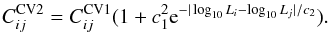 (A.4)Here
c1 is the fractional prior uncertainty in
the bias and c2 is its correlation length in
log 10L. The fiducial parameters taken are
c1 =
0.5 (50% scatter in the bias model) and c2 = 2 (2 dex
correlation length). As always with priors, these parameters are somewhat ad hoc, but
despite this drawback we expect that a procedure with a range of bias models is more
likely to be able to approximate the real Universe than a fixed-bias case
(
(A.4)Here
c1 is the fractional prior uncertainty in
the bias and c2 is its correlation length in
log 10L. The fiducial parameters taken are
c1 =
0.5 (50% scatter in the bias model) and c2 = 2 (2 dex
correlation length). As always with priors, these parameters are somewhat ad hoc, but
despite this drawback we expect that a procedure with a range of bias models is more
likely to be able to approximate the real Universe than a fixed-bias case
( ) or
the assumption of no cosmic variance at all.
) or
the assumption of no cosmic variance at all.
There are thus 3 possible models for the incorporation of cosmic variance in the narrow-band luminosity function:
-
No inclusion of cosmic variance (Cij = 0).
-
The simple, luminosity-independent bias model (
).
-
A random suite of luminosity-dependent bias models (
 ).
).
The slitless surveys have a very different geometry: they probe tiny areas (e.g. the WFC3 detector covers only 4.8 arcmin2), but they have a very long contribution in the radial direction and usually have many more independent fields (Nf = 29 for WISP). For the 0.3 <z< 0.9 and 0.9 <z< 1.5 slices, the predicted cosmic variance diagonal covariances for WISP are 0.0020 and 0.0014 respectively. The WISP luminosity function includes the cosmic variance term, although the fitting procedure used here does not include the cosmic variance covariance between luminosity bins. We have not attempted to add these in, as the additional ~4% standard deviation is negligible.
Appendix B: Poisson error bars
This Appendix considers the asymmetry of the Poisson error bar in the context of constructing a likelihood function for the Hα luminosity function for Model 3. The procedure was inspired by applications in cosmic microwave background data analysis, where the anisotropy power spectrum has asymmetric (in that case, χ2-shaped) error bars (Verde et al. 2003). A common example is in power spectrum estimation, where the overall fit can be biased downward if symmetric error bars are assumed because the lower data points have smaller error bars and pull the fit. For this reason, parameterized forms of the asymmetry are common in reporting likelihood functions in the cosmic microwave background community (see e.g. Bond et al. 1998, 2000; Verde et al. 2003). A similar phenomenon can occur in fitting a luminosity function: the Poisson error bar on a data point that fluctuates downward is smaller than on a point that fluctuates upward, so fits to the raw luminosity function that treat this error as symmetric will be biased toward lower φ(L,z). As an extreme example, the likelihood function will even allow a finite likelihood for φ(L,z) < 0, which is clearly unphysical. On the other hand, treating the error on log 10φ(L,z) as symmetric will bias φ(L,z) upward, since data points that fluctuate upward will have smaller error bars in log-space.
If the Hα
luminosity function measurements contained only Poisson errors, then the log-likelihood
for a point with N objects, a survey volume ΔV, and a bin width
ΔL is
 (B.1)where
λ = φ
ΔL ΔV is the expected number of
objects. The maximum likelihood point is at λ = N, and so the log-likelihood
relative to the maximum is
(B.1)where
λ = φ
ΔL ΔV is the expected number of
objects. The maximum likelihood point is at λ = N, and so the log-likelihood
relative to the maximum is 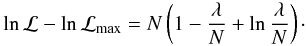 (B.2)The
estimate of the luminosity function is
(B.2)The
estimate of the luminosity function is  , and the
estimate of its uncertainty is
, and the
estimate of its uncertainty is  ,
so this can be re-written as
,
so this can be re-written as 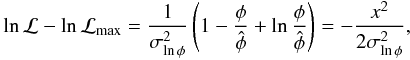 (B.3)where
we have defined the re-scaled parameter x as follow:
(B.3)where
we have defined the re-scaled parameter x as follow: 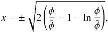 (B.4)with
the + sign used if
(B.4)with
the + sign used if
 and the − sign if
 .
We note that the argument of the square root is always positive (or 0 if
.
We note that the argument of the square root is always positive (or 0 if
 ),
and that x is
actually an analytic function of
),
and that x is
actually an analytic function of  ,
, ![Mathematical equation: \appendix \setcounter{section}{2} \begin{eqnarray} x = \pm\sqrt{2[y-\ln(1+y)]} = y - \frac13y^2 + \frac7{36}y^3 - ... \label{eq:xy-P} \end{eqnarray}](/articles/aa/full_html/2016/06/aa27081-15/aa27081-15-eq305.png) (B.5)The
real error bars need not have the same asymmetry as the Poisson distribution in the cases
where they are dominated by other terms (e.g. cosmic variance). We therefore test for the
sensitivity of the results to the assumed fitting scheme.
(B.5)The
real error bars need not have the same asymmetry as the Poisson distribution in the cases
where they are dominated by other terms (e.g. cosmic variance). We therefore test for the
sensitivity of the results to the assumed fitting scheme.
The covariance matrix C is
re-written in terms of x, and the log-likelihood surface is taken to be
quadratic, ![Mathematical equation: \appendix \setcounter{section}{2} \begin{eqnarray} \chi^2 = -2\ln{\cal L} + 2\ln{\cal L}_{\rm max} = \sum_{ij} [{\tens C}^{-1}]_{ij} x_i x_j. \end{eqnarray}](/articles/aa/full_html/2016/06/aa27081-15/aa27081-15-eq307.png) (B.6)This
approach has the advantage that with one switch in the fitting code, the error asymmetry
may be treated in 4 ways:
(B.6)This
approach has the advantage that with one switch in the fitting code, the error asymmetry
may be treated in 4 ways:
-
Poisson: this uses Poisson-shaped errors (Eq. (B.5)).
-
Symmetric-linear: this uses symmetric errors in φ, by setting x = y.
-
Symmetric-log: this uses symmetric errors in log 10φ or lnφ, by setting x = ln(1 + y).
-
Symmetric-native: this uses errors symmetric in either φ or lnφ, depending on which was reported by the analysis team.
The Poisson shape for the error bars is probably the most realistic in the bins with small numbers of galaxies, but due to the contribution of other errors it is not exact. Therefore we consider other shapes as well (see Appendix C).
Appendix C: Variations and robustness of Model 3
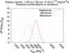 |
Fig. C.1 Posterior probability distribution for the number of galaxies at F> 2 × 10-16 erg cm-2 s-1 and in the wavelength range 1.25–1.80 μm (redshift 0.90–1.74), for reference Model 3 and its extreme combinations of modifications considered (see text). |
Fit parameters for the various models considered.
In order to assess the robustness of Model 3, we re-ran the fits modifying some of the key aspects of the data handling. The reference model is based on (i) use of all datasets; (ii) the broken power law model for the luminosity function; (iii) the CV2 cosmic variance prescription; (iv) the Poisson error bar asymmetry model; (v) integration over luminosity and redshift bins using NG = 3; (vi) HiZELS aperture corrections assuming a 0.3 arcsec half-light radius for all sources; and (vii) the [N ii]/Hα ratio assumed in the input publications. We vary the reference assumptions (functional function, CV, NG, error bars) and we also considered extreme combinations of modifications to come up with bounding optimistic (MAX) or conservative (MIN) estimates of the HαLF. Relative to the reference fit, the MAX fit used the combination of fits to the bin centre; error bars symmetric in log φ; and WISP+NICMOS data only. The MIN fit used the combination of error bars symmetric in φ; and HiZELS+WISP data only. The main types of variations considered, and results of the fit are listed in Table C.1. We consider the predictions of the models for the number of galaxies N2 above 2 × 10-16 erg cm-2 s-1 and in the Hα redshift range (0.9 <z< 1.74).
The fits with more simplistic treatment of the finite bin width (using NG = 1 and the luminosity function at z = (zmin + zmax) /2 and log 10L = (log 10Lmin + log 10Lmax) / 2) lead to higher predicted counts. This is the result of Eddington-like biases: for a steeply falling luminosity function10, a bin of width Δlog 10L × Δz contains more galaxies than would be predicted based on the luminosity function at the bin centre. The reference fit corrects this effect by incorporating it in the model. The NG = 5 case was run as a convergence test, and shows ≪1σ changes. The differences between the cases indicate the significance of different ways of treating finite bin size. The uncertainties are largest for the NICMOS data since large bins in both log L and z were used in the NICMOS studies (Yan et al. 1999; Shim et al. 2009). The effect of this treatment is smallest for HiZELS since there is no averaging over redshifts and the log L bins are narrow.
The choice of cosmic variance treatment (CV1 versus CV2) matters little (≪1σ) in the integrated counts in the Euclid range FHα> 2 × 10-16 erg cm-2 s-1 from switching between these two models, although the faint-end slope changes by 1σ.
A bigger difference arises when the cosmic variance is artificially turned off; this causes the predicted number of galaxies to go up by 2σ. This behaviour is driven by the three lowest-luminosity HiZELS points at z = 0.84, which have small formal error bars (0.03 or 0.04 dex) and are actually above the WISP counts.
The treatment of error bar asymmetries pulls the fits in the expected direction: treating the error bars as symmetric in φ leads to a lower result by almost 2σ, and treating them as symmetric in log 10φ leads to a higher result by almost 2σ, relative to the Poisson-shaped error bar. The Poisson shape (reference) is the best-motivated form, since we know that a major contribution to the luminosity function error has this shape, but many past fits have been done with one of the two other shapes, and we do not have a clear understanding of the asymmetry of the systematic errors.
We performed fits excluding each of the 3 major input samples Since the narrow-band HiZELS Hα luminosity function is the lowest in the Euclid range, and the NICMOS results are the highest, exclusion of HiZELS moves the predicted number of galaxies up, whereas exclusion of NICMOS moves it down. The difference between the highest and lowest result in this sample jack-knife is 0.161 dex. This suggests that systematic errors are contributing to the differences of these curves and that caution should be exercised in interpreting joint fits.
The alternative fitting functions, especially the Schechter function, lead to slightly greater number densities than the reference (broken power law). This is because they incorporate an exponential cutoff, and hence the existence of a few very bright galaxies (>5 L⋆, particularly in the NICMOS data) pulls the characteristic luminosity to larger values and increases the number of objects in the intermediate range (~2 L⋆). However, this same feature of the Schechter law means that it is a poor fit to the NICMOS observations, and it is disfavoured relative to the broken power law model by Δχ2 = 20, and in any case the effect in our fiducial range (FHα> 2 × 10-16 erg cm-2 s-1, 0.90 <z< 1.74) is only 1σ.
The reference aperture correction for HiZELS assumes a half-light radius of 0.3 arcsec, which is consistent with objects near the flux limit of WFIRST-AFTA (see Colbert et al. 2013, Fig. 11). We have tried two variations on this: an extreme case of turning the aperture correction off, and a case of implementing a variable galaxy size in accordance with the fit provided in Sect. 4.2 of Colbert et al. (2013)11. The changes in the number of objects in the range 0.90 <z< 1.74 and at FHα> 2 × 10-16 erg cm-2 s-1 are − 10% and − 2% for the no aperture correction and Colbert et al. (2013) correction cases, respectively.
The last modelling assumption that was varied was the assumed
[N ii]/Hα ratio, which enters because at low resolution
[N ii] and Hα are blended; thus Hα+[N ii] is
measured, and Hα is inferred under some assumed prescription for the
line ratio. The reference model is based on the Hα luminosity function
directly from the published papers: this means that the assumed
[N ii]/Hα is that in the published papers (0.41 for NICMOS
and WISP; in HiZELS a variable ratio was used but the reported median is 0.33). Here
[N ii] includes both doublet members, 6548 Å and 6583 Å; 75.4% of the flux in
the stronger 6583 Å line (Storey & Zeippen
2000). This ratio is common at low redshifts, however a range of values is
observed, and in high-redshift galaxies the [N ii]/Hα ratio is often observed
to be smaller. We have therefore investigated what happens under alternate assumptions
regarding the [N ii]/Hα ratio. First, the luminosities were converted
back to LHα + [ NII ] using
the stated median ratios in each input paper. Then the Hα+[N ii]
luminosity function was written as ![Mathematical equation: \appendix \setcounter{section}{3} \begin{eqnarray} \phi_{{\rm H}\alpha + [{\rm NII}]}(L_{{\rm H}\alpha + [{\rm NII}]}) = \int \phi_{{\rm H}\alpha}(L_{{\rm H}\alpha}) p(x|L_{{\rm H}\alpha}) \left.\frac{\partial L_{{\rm H}\alpha}}{\partial x}\right|_{L_{{\rm H}\alpha + [{\rm NII}]}} \,{\rm d}x, \label{eq:intquad} \end{eqnarray}](/articles/aa/full_html/2016/06/aa27081-15/aa27081-15-eq369.png) (C.1)where
x =
log 10(L6583/LHα)
is the relative line strength in dex and LHα =
LHα + [ NII ]/ (1 +
10x/ 0.754). We built
two alternative models for the [N ii]/Hα ratio based on the ⟨ z ⟩ = 2.3 BPT diagram of
star-forming galaxies (Steidel et al. 2014). One
model (altNII1) uses the median [N ii]/Hα ratio from the Steidel et al. (2014) sample, x = − 0.90 dex (see Fig.
5). The other (altNII2) assumes a lognormal distribution; since the 84th percentile
(+ 1σ) of
the [N ii]/Hα ratio corresponds to x = − 0.57 dex, we choose a
median at −0.90 dex and a
scatter of σx = 0.33 dex.
(C.1)where
x =
log 10(L6583/LHα)
is the relative line strength in dex and LHα =
LHα + [ NII ]/ (1 +
10x/ 0.754). We built
two alternative models for the [N ii]/Hα ratio based on the ⟨ z ⟩ = 2.3 BPT diagram of
star-forming galaxies (Steidel et al. 2014). One
model (altNII1) uses the median [N ii]/Hα ratio from the Steidel et al. (2014) sample, x = − 0.90 dex (see Fig.
5). The other (altNII2) assumes a lognormal distribution; since the 84th percentile
(+ 1σ) of
the [N ii]/Hα ratio corresponds to x = − 0.57 dex, we choose a
median at −0.90 dex and a
scatter of σx = 0.33 dex.
In the altNII1 model, the number of objects in the range 0.90 <z< 1.74 and at FHα> 2 × 10-16 erg cm-2 s-1 increases by 45%; the weaker assumed [N ii] results in larger inferred Hα luminosities, and this effect is amplified by the steep luminosity function. On the other hand, for the altNII2 model, which includes scatter as well, we find a source density only 29% above the reference model; the reduction occurs because the scatter in [N ii] results in an Eddington-like bias that is corrected by Eq. (C.1). While an improvement over the reference model in some ways, the 29% increase in the altNII2 model may be an overestimate, since (i) it applies a correction based on the ⟨ z ⟩ = 2.3 BPT diagram even at lower redshifts; and (ii) the correction procedure is not technically correct for HiZELS,
which has a variable assumed [N ii] fraction and which may include only part of the Hα+[N ii] complex in its band12. There may also be differences (whose impact has undetermined sign) between the rest-frame ultraviolet selection in Steidel et al. (2014) and Hα selection. Based on these considerations, we are not using it to replace the reference model.
Finally, it is seen that the central values of the MIN and MAX fits for the number of objects in the range 0.90 <z< 1.74 and at FHα> 2 × 10-16 erg cm-2 s-1 differ by a factor of 2 (see Table C.1).
All Tables
Empirical Schechter parameters for the various surveys considered, ordered by redshift.
Redshift distributions for a range of limiting fluxes (in units of 10-16 erg cm-2 s-1) from the 3 empirical Models (1, 2, 3).
All Figures
|
Fig. 1 Hα LFs at various redshifts. The dotted lines mark the nominal flux limit of Euclid (3 × 10-16 erg cm-2 s-1) in the lower bound of each redshift range. Observed Schechter LFs are shown as thin lines and squares in the observed luminosity range and listed in the labels. For comparison, the LFs from Empirical Models 1, 2, and 3 are shown (in yellow, cyan, and pink, respectively) as thick lines in the same redshift range (shown in the two extremes of each redshift bin). |
| In the text | |
|
Fig. 2 Hα LFs empirical Schechter parameters (using the same colours as Fig. 1) as a function of redshift (at the center redshift of each surveys), along with the evolution of parameters in the models. |
| In the text | |
|
Fig. 3 Residuals to the Hα luminosity function fits for Model 3, plotted as a function of observed-frame Hα flux at the bin centre (horizontal axis). All redshifts are plotted together. The green lines show the fit line and factors of 2 above and below. The error bars shown do not include the cosmic variance, which is included in the fit but is highly correlated across luminosity bins. |
| In the text | |
|
Fig. 4 Left panel: cumulative Hα number counts, integrated over the redshift ranges 0.7 <z< 1.5 (WISP range). The observed counts from the WISP survey (Colbert et al. 2013) are shown (blue circles) and from new WISP analysis by Mehta et al. (2015; cyan circles), and compared to the empirical Model 1, 2, and 3, (blue, black and red lines, respectively). Also shown (as dotted lines and empty squares) are the counts obtained integrating the observed LFs (see legend) in the same redshift range. Right panel: same cumulative Hα number counts compared to the predictions from L12 mocks (green dashed and solid lines using intrinsic and extincted Hα fluxes, respectively) and GP14 mocks (dark and light grey for H< 27 and H< 24 mocks, respectively). |
| In the text | |
|
Fig. 5 Hα redshift distribution above various flux thresholds (from 0.5 × 10⁻¹⁶ erg cm-2 s-1 to 3 × 10-16 erg cm-2 s-1, from top to bottom panels). Observed redshift distributions are indicated with open circles, while data obtained integrating LFs are shown with squares. HaLF predictions from Model 1, 2, 3 are shown as thick solid lines. The predictions from L12 mocks (green dashed and solid lines using intrinsic and extincted Hα fluxes, respectively) and GP14 mocks (dark and light grey for H< 27 and H< 24 mocks, respectively) are also shown. |
| In the text | |
|
Fig. 6 Hα luminosity density of the Universe as a function of redshift. The solid thick lines show the total luminosity density, whereas the thin solid curves show the luminosity density for emitters at F> 10-16 erg cm-2 s-1 (upper set of curves) and F> 3 × 10-16 erg cm-2 s-1 (lower set of curves). The different colours are codes for each model (blue, Model 1; black, Model 2; and red, Model 3). Also shown is the calculation of total Hα luminosity density based on the star formation histories of Madau & Dickinson (2014, green dashed) and Behroozi et al. (2013, gray dashed and shaded area). On the right axis we report also the SFR density scale for a Chabrier IMF. |
| In the text | |
|
Fig. C.1 Posterior probability distribution for the number of galaxies at F> 2 × 10-16 erg cm-2 s-1 and in the wavelength range 1.25–1.80 μm (redshift 0.90–1.74), for reference Model 3 and its extreme combinations of modifications considered (see text). |
| In the text | |
Current usage metrics show cumulative count of Article Views (full-text article views including HTML views, PDF and ePub downloads, according to the available data) and Abstracts Views on Vision4Press platform.
Data correspond to usage on the plateform after 2015. The current usage metrics is available 48-96 hours after online publication and is updated daily on week days.
Initial download of the metrics may take a while.