| Issue |
A&A
Volume 589, May 2016
|
|
|---|---|---|
| Article Number | A98 | |
| Number of page(s) | 15 | |
| Section | Extragalactic astronomy | |
| DOI | https://doi.org/10.1051/0004-6361/201527642 | |
| Published online | 19 April 2016 | |
Individual power density spectra of Swift gamma-ray bursts ⋆
1
Department of Physics and Earth SciencesUniversity of Ferrara,
via Saragat 1,
44122
Ferrara,
Italy
e-mail:
This email address is being protected from spambots. You need JavaScript enabled to view it.
2
ICRANet, P.zza della Repubblica 10, 65122
Pescara,
Italy
3
INAF–Istituto di Astrofisica Spaziale e Fisica Cosmica di Bologna,
via Gobetti 101, 40129
Bologna,
Italy
Received: 26 October 2015
Accepted: 10 March 2016
Abstract
Context. Timing analysis can be a powerful tool with which to shed light on the still obscure emission physics and geometry of the prompt emission of gamma-ray bursts (GRBs). Fourier power density spectra (PDS) characterise time series as stochastic processes and can be used to search for coherent pulsations and, more in general, to investigate the dominant variability timescales in astrophysical sources. Because of the limited duration and of the statistical properties involved, modelling the PDS of individual GRBs is challenging, and only average PDS of large samples have been discussed in the literature thus far.
Aims. We aim at characterising the individual PDS of GRBs to describe their variability in terms of a stochastic process, to explore their variety, and to carry out for the first time a systematic search for periodic signals and for a link between PDS properties and other GRB observables.
Methods. We present a Bayesian procedure that uses a Markov chain Monte Carlo technique and apply it to study the individual PDS of 215 bright long GRBs detected with the Swift Burst Alert Telescope in the 15−150 keV band from January 2005 to May 2015. The PDS are modelled with a power-law either with or without a break.
Results. Two classes of GRBs emerge: with or without a unique dominant timescale. A comparison with active galactic nuclei (AGNs) reveals similar distributions of PDS slopes. Unexpectedly, GRBs with subsecond-dominant timescales and duration longer than a few tens of seconds in the source frame appear to be either very rare or altogether absent. Three GRBs are found with possible evidence for a periodic signal at 3.0–3.2σ (Gaussian) significance, corresponding to a multi-trial chance probability of ~1%. Thus, we found no compelling evidence for periodic signal in GRBs.
Conclusions. The analogy between the PDS of GRBs and of AGNs could tentatively indicate similar stochastic processes that rule BH accretion across different BH mass scales and objects. In addition, we find evidence that short dominant timescales and duration are not completely independent of each other, in contrast with commonly accepted paradigms.
Key words: gamma-ray burst: general / methods: statistical
Full Tables 1−4 are only available at the CDS via anonymous ftp to cdsarc.u-strasbg.fr (130.79.128.5) or via http://cdsarc.u-strasbg.fr/viz-bin/qcat?J/A+A/589/A98
© ESO, 2016
1. Introduction
It is an observationally established fact that long gamma-ray bursts (GRBs), or at least most of them, are associated with the collapse of some type of hydrogen–stripped massive stars (Woosley & Bloom 2006; Hjorth 2013).
The most important and open questions, however, concern the nature of the ejecta and their magnetisation degree, where and how energy dissipation takes place, and the radiation mechanism(s). All these questions are intertwined so that explaining all the observed properties in a consistent picture is challenging.
Sample of 215 GRBs.
Generally, several types of dissipation processes have been proposed: i) the so–called internal shock (IS) model (Rees & Meszaros 1994; Narayan et al. 1992), in which the kinetic energy of a baryon load is dissipated into gamma rays through shocks that take place far away from the Thomson photosphere, at 1014–1016 cm; ii) the photospheric models, in which the dissipation occurs near the photosphere, and where a Planckian spectrum is modified by some heating and Compton scattering (Rees & Mészáros 2005; Pe’er et al. 2006; Thompson et al. 2007; Derishev et al. 1999; Rossi et al. 2006; Beloborodov 2010; Titarchuk et al. 2012; Giannios 2008; Mészáros & Rees 2011; Giannios 2012); iii) magnetised ejecta (σ = B2/ 4πΓρc2> 1) dissipate their energy at distances similar to those of IS (Lyutikov & Blandford 2003; Zhang & Yan 2011; Beniamini & Granot 2015).
The study of time variability through Fourier power density spectra (PDS; see van der Klis 1989; Vaughan 2013 for reviews) can help to constrain the energy dissipation in GRBs as a stochastic process and also the dissipation region (Titarchuk et al. 2007). Owing to the statistical noise of counting photons in the detector (van der Klis 1989), in the GRB literature only average PDS of long GRBs were studied so far (Beloborodov et al. 2000; Ryde et al. 2003; Guidorzi et al. 2012; Dichiara et al. 2013a). The average PDS can be modelled with a power-law extending from a few 10-2 to ~1 Hz. Power-law indexes vary from ~1.5 to ~2 depending on the energy passband, with steeper PDS corresponding to softer photons. The smooth behaviour of the PDS averaged over a large number of GRBs facilitates modelling. At the same time, it prevents studying the individual properties of GRBs, whose light curves are non–stationary, short–lived time series. Specifically, we cannot search for either periodic, quasi-periodic signals, or correlations with other intrinsic properties (e.g. related to the energy spectrum). The need to overcome these limitations calls for a proper statistical treatment of individual PDSs.
In this work we develop a Bayesian Markov chain Monte Carlo technique that builds upon the procedure outlined by Vaughan (2010, hereafter V10). We then apply it to model the PDS of individual GRBs and study the statistical properties of an ensemble of GRBs detected in the 15−150 keV energy band with the Burst Alert Telescope (BAT; Barthelmy et al. 2005) onboard the Swift satellite (Gehrels et al. 2004). We chose the Swift catalogue to ensure a large homogeneous sample; in addition, thanks to the large portion (~30%) of GRBs with measured redshift, we can access a correspondingly larger set of intrinsic properties. The same technique was recently adopted for studying a selected sample of bright short GRBs (Dichiara et al. 2013b). A very similar approach was used for studying the outbursts from magnetars (Huppenkothen et al. 2013) and for searching them for quasi–periodic oscillations (QPOs; Huppenkothen et al. 2014a,b).
The advantage of studying individual vs. averaged PDS is threefold: i) we directly probe the variety of stochastic processes taking place during the gamma-ray prompt emission; ii) we search for possible connections between PDS and other key properties of the prompt emission, such as the intrinsic (i.e. source rest-frame) peak energy Ep,i, and the isotropic–equivalent radiated energy, Eiso, involved in the eponymous correlation (Amati et al. 2002); iii) we search for occasional features emerging from the PDS continuum, such as coherent pulsations or QPOs, which, if any, would be completely washed out by averaging the PDS of many different GRBs. In a companion paper (Dichiara et al. 2016, hereafter D16) we focus on the Ep,i–PDS correlation and its theoretical implications for a large number of GRBs with known redshift detected by several past and present spacecraft.
The paper is organised as follows: the data selection and analysis are described in Sect. 2. Section 3 reports the results, which are discussed in Sect. 4. The description of the technique adopted for the PDS modelling is reported in Appendix A. Uncertainties on the best–fitting parameters are given at 90% confidence for one parameter of interest, unless stated otherwise.
2. Data analysis
2.1. Data selection
From an initial sample of 961 GRBs detected by BAT from January 2005 to May 2015 we selected those whose time profiles were entirely covered in burst mode, that is, with the finest time resolution available. As a consequence, GRBs discovered offline were excluded. For the surviving 877 GRBs we extracted mask-weighted, background-subtracted light curves with a uniform binning time of 4 ms in two separate energy channels, 15−50 and 50−150 keV, and in the total passband 15−150 keV. As in Guidorzi et al. (2012, hereafter G12), we did not split the full passband into finer energy bands to ensure a good signal–to–noise ratio (S/N) for the light curves of most GRBs.
Light curves were extracted from the corresponding BAT event files. The latter were processed with the HEASOFT package (v6.13) following the BAT team threads1. Mask-weighted light curves were extracted using the ground-refined coordinates provided by the BAT team for each burst through the tool batbinevt. We built the BAT detector quality map of each GRB by processing the next earlier enable or disable map of the detectors. Light curves are expressed as background-subtracted count rates per fully illuminated detector for an equivalent on-axis source.
For each of these GRBs we calculated the PDS following the procedure described in G12. The final selection was made by imposing a threshold of S/N ≥ 30 on the total 15−150 keV fluence collected in the time interval selected for the PDS extraction. The choice for this particular value for the S/N threshold is explained in Sect. 3. From the 218 GRBs that remained at this stage, we selected the long bursts by requiring T90> 3 s, where T90 were taken from the second BAT catalogue (Sakamoto et al. 2011) or from the corresponding BAT-refined circulars for the most recent GRBs not included in the catalogue. This requirement on the GRB duration excluded the only three short bursts that had fulfilled the S/N criterion: 051221A, 060313, and 100816A. We verified that no short GRB with extended emission (Norris & Bonnell 2006; Sakamoto et al. 2011) with T90> 3 s slipped into the long-duration sample.
2.2. PDS calculation
Like G12, we determined the T7σ interval, which spans from the first and the last time bins whose rates exceed by ≥ 7σ the background. For most Swift GRBs its duration is very similar to that of T90. The PDS was then calculated on a 3 × T7σ long interval with the same central time as the T7σ sample, as the result of a trade–off between covering the overall GRB profile and optimising the S/N (G12). Table 1 reports the time intervals used for each of the 215 GRBs along with the corresponding T7σ and T90. The latter values were taken either from the official BAT catalogue (Sakamoto et al. 2011) when available, or otherwise from the BAT refined GCN circulars. Reporting both the selected time intervals and T7σ is not redundant because for a fraction of GRBs 3 × T7σ was longer than the available data in burst mode.
The Leahy normalisation was adopted for the PDS, in which the white-noise level that is due to uncorrelated statistical noise has a value of 2 for pure Poissonian noise (Leahy et al. 1983).
For each light curve we initially calculated the PDS by keeping the original minimum binning time of 4 ms, which corresponds to a Nyquist frequency of 125 Hz. After we ensured that no high–frequency (f ≳ 10 Hz) periodic feature stood out from the continuum, we decided to cut down the long computational time demanded by Monte Carlo simulations by binning up the light curves to 32 ms, equivalent to a Nyquist frequency fNy = 15.625 Hz. We did not adopt the potentially alternative approach of binning up along frequency after we noted that the corresponding distribution of power at high frequencies significantly deviated from the expected  , where M is the re−binning factor (van der Klis 1989). We investigated the cause for this and found out that there are two independent reasons: one is related to the question of the correlated power at low frequencies and is discussed in the shortcomings of our technique (Sect. A.1); the other reason is that the mask-weighted light curve of a BAT GRB covers time intervals during which the spacecraft rapidly slewed because of the GRB itself: consequently, the mask-weighted rates are calculated from time-varying weights that depend on the GRB direction relative to the spacecraft. This causes a pattern in the time series of the uncorrelated Gaussian uncertainties of rates, and makes the resulting rate light curves heteroscedastic. We simulated light curves with the same pattern in the variance and obtained PDS exhibiting the same behaviour. However, as long as the PDS is kept unbinned, this problem does not affect the results at a statistically significant level.
Unless stated otherwise, the PDS hereafter discussed were calculated in this way. Neither white-noise subtraction nor frequency re–binning was applied to the original PDS.
2.3. PDS modelling
Fitting the observed PDS with a given model requires knowing the statistical distribution followed by the PDS at each frequency. For instance, adopting standard least-squares optimisation techniques is conceptually incorrect for an unbinned PDS because power fluctuates according to a χ2, that is, more wildly than a Gaussian variable. We therefore devised a proper treatment that expands upon the procedure outlined by V10 with some changes. We refer to Appendix A for a detailed description.
We considered two different models: the first is a simple power-law (pl) plus the white-noise constant, 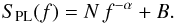 (1)For each PDS we first tried to fit the PDS with Eq. (1) with the following free parameters: the normalisation constant N (we used log N as the free parameter, see Appendix A), the power-law index α (> 0), and the white-noise level B.
However, for many GRBs the PDS clearly showed evidence for a break in the power-law. We therefore considered a model of a power-law with a break below which the slope is constant, which is hereafter called bent power-law (bpl) model, ![Mathematical equation: \begin{equation} S_{\rm BPL}(f) = N\,\left[1 + \left(\frac{f}{f_{\rm b}}\right)^{\alpha}\right]^{-1} + B , \label{eq:mod_bpl} \end{equation}](/articles/aa/full_html/2016/05/aa27642-15/aa27642-15-eq76.png) (2)which is equivalent to the pl model in the limit f ≫ fb. Below the break frequency, f<fb, the power density flattens. We did not adopt the more complex broken power-law model such as that of Eq. (1) in G12 that was used for the average PDS, which has an additional power-law index for the low–frequency range. The reason is that the PDS of individual GRBs fluctuate more wildly around the model than the average PDS of a sample of GRBs, simply because the fewer the degrees of freedom of a χ2 distribution, the higher the ratio between variance and expected value. This makes the fit with a broken power-law very poorly constrained for most PDS of our sample because it adds an additional free parameter, five instead of four. On top of this, a flat power density at low frequencies (f ≪ 1 /T, where T is the GRB duration) is also expected for a time-limited event, such as the light curve of a GRB. In Appendix A we discuss the plausibility of these models for GRBs in more detail, along with the applicability limits and possible problems.
(2)which is equivalent to the pl model in the limit f ≫ fb. Below the break frequency, f<fb, the power density flattens. We did not adopt the more complex broken power-law model such as that of Eq. (1) in G12 that was used for the average PDS, which has an additional power-law index for the low–frequency range. The reason is that the PDS of individual GRBs fluctuate more wildly around the model than the average PDS of a sample of GRBs, simply because the fewer the degrees of freedom of a χ2 distribution, the higher the ratio between variance and expected value. This makes the fit with a broken power-law very poorly constrained for most PDS of our sample because it adds an additional free parameter, five instead of four. On top of this, a flat power density at low frequencies (f ≪ 1 /T, where T is the GRB duration) is also expected for a time-limited event, such as the light curve of a GRB. In Appendix A we discuss the plausibility of these models for GRBs in more detail, along with the applicability limits and possible problems.
To establish whether a bpl provides a statistically significant improvement in the fit of a given PDS of a GRB with respect to a pl, we used the likelihood ratio test (LRT) in the Bayesian implementation described by V10 (see Eq. (A.9) and Appendix A for details). In a pure Bayesian approach, the Bayes factor should be used as an alternative to the LRT (Kass & Raftery 1995): model selection does not require the choice of any test statistic, but depends on the likelihood marginalised (not maximised) over the joint prior of the parameters. The dependence on the parameters is thus removed at the cost of computationally demanding multi-dimensional integrations and upon selection of appropriate priors for the parameters2.
For the LRT test, we accepted the bpl model when the probability of chance improvement was lower than 1%. Figure 1 illustrates two examples of PDS and their best–fitting models, one for each model.
The choice of 1% for the LRT test significance was the result of a trade–off between type I and type II errors, also based on a set of preliminary simulated light curves. For lower values, a number of PDS that displayed a clear–cut break by visual inspection, and for which fitting with bpl constrained the parameters reasonably well, did not pass the test (too many type II errors). On the other hand, adopting significance values higher than 1% turned into numerous bpl–modelled PDS with very poorly constrained parameters (type I errors). To calibrate the LRT threshold independently of the data, we also used two types of synthetic light curves filled with pulses that had (i) a narrow distribution of characteristic timescales; (ii) a broad distribution of timescales, one tenth to several ten seconds. Peak times were assumed to be either lognormally or exponentially distributed, in agreement with observed distributions (e.g. see Baldeschi & Guidorzi 2015, and references therein). For the synthetic curves (i) we ensured that our procedure required bpl, whereas no such preference was shown for the curves (ii). The final choice of 1% in our sample gave only a handful of GRBs, for which we had to force the pl model, although the LRT test had formally rejected it. The reason was that the bpl parameters could not be constrained (type I errors). Just a few is also consistent with what is expected from an equally numerous set with 1% probability that bpl is mistakenly preferred to pl.
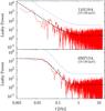 |
Fig. 1 Examples of individual PDS. Dashed lines show the corresponding best–fitting model. Dotted lines show the 3σ threshold for periodic pulsations. Top: the PDS of 110119A can be fitted with a simple pl model and background. Bottom: fitting the PDS of 050713A significantly improves with a bpl model. |
3. Results
Table 2 reports for each of the 215 selected GRBs the means and standard deviations of the posterior distributions of the parameters of the corresponding model and the p-values of each of the relevant statistics introduced in Appendix A, in the 15−150 keV band. Likewise, Tables 3 and 4 report the analogous information for the energy channels 15−50 and 50−150 keV, respectively. Given that we did not re-bin the PDS along frequency and extracted the PDS out of a single time interval, we minimised the log-likelihood of Eq. (A.7) with M = 1. The number of GRBs whose PDS are best fit with bpl is 75, 60, and 75 for the total band, the 15−50 and the 50−150 keV channels, respectively, that is, about one-third of the sample.
To limit the effects of poorly constrained parameters in the parameters’ distributions, we selected the GRBs with well-constrained power-law indexes, σ(α) < 0.5 (both models), and an analogous condition on log (fb), σ(log (fb)) < 0.3, corresponding to a factor-of-2 uncertainty on fb for the total band. The sample of 215 GRBs shrank to a sub-sample of 198 with well-constrained parameters. Within this restricted sample, the fraction of GRBs best fit with bpl is 67/198, which is still one-third.
We first assessed the individual and global goodness of the best-fitting models through the distributions of the p-values associated with the Anderson-Darling (AD) and Kolmogorov-Smirnov (KS) statistics (Appendix A), finding a mean and standard deviation of pAD = 0.69 ± 0.26 and pKS = 0.66 ± 0.26, respectively. The distributions of both p-values are incompatible with a uniform one in the [ 0:1 ] interval, being skewed towards 1. The explanation likely lies in the shortcomings of the procedure (Sect. A.1). The lowest individual p-values are a few percent, in agreement with what is expected of a sample of 200 elements, except for 140209A, for which both p-values were ~0.1%. Likewise, the p-values associated with the TR statistic that were used to search for periodic features (see V10; Appendix A) are compatible with being uniformly distributed, as indicated by the p-value of 0.51 of a KS test.
Best–fitting model along with means and standard deviations of the parameters’ posterior distributions for each GRB of the sample of 215 events in the total 15−150 keV energy band.
Best–fitting model along with means and standard deviations of the parameters’ posterior distributions for each GRB of the sample of 215 events in the 15−50 keV energy band.
Best–fitting model along with means and standard deviations of the parameters’ posterior distributions for each GRB of the sample of 215 events in the 50−150 keV energy band.
We investigated whether the samples that were fit with different models exhibited a significantly different S/N: a KS test on the two S/N distributions gave an 11% probability of being drawn from a common population. We were led to adopt the threshold of S/N ≥ 30 for the sample selection because when we had included GRBs below it in a previous attempt, the fraction of pl–best fit GRBs increased notably and the two S/N distributions became very different. This was interpreted as evidence that GRBs with S/N< 30 were just too noisy and that the stronger preference for pl was a mere S/N artefact. Similarly, no evidence for a different T90 distribution was found between the two classes. We found a very weak indication that bpl GRBs on average have fewer pulses per GRB, given a KS-test probability of 7% that the two classes have the same number of pulses. The number of pulses of each GRB, reported in Table 1, had preliminarily been determined by applying the MEPSA code (Guidorzi 2015) to the 15−150 keV band profiles.
3.1. White noise
For the prior of the white-noise level B we adopted a Gaussian distribution centred on 2, expected for pure Poissonian noise, with σ = 0.2, thus allowing deviations as large as ~10%. This is a conservative approach, given the relatively little extra-Poissonian noise that affects BAT as a result of the detector itself and of its electronics (Rizzuto et al. 2007). Another possible source of variance suppression is the detector dead time for particularly bright GRBs. In this case the variance is suppressed by a factor (1 − μτ)2, where μ is the average count rate in an individual detector unit and τ ~ 100 μs3 is the BAT dead time. A 10% dead-time suppression would imply an average rate of several thousand counts/s in each BAT detector module, which is way higher than the 700 events/s of the brightest events (Barthelmy et al. 2005). Therefore, our choice for the B prior is very conservative, but is nonetheless useful to avoid unphysical values.
The resulting distribution is shown in Fig. 2 along with the prior distribution.
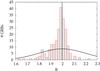 |
Fig. 2 Distribution of the white-noise level B. The vertical dashed line shows the pure Poissonian case. The solid Gaussian shows the prior distribution on B. |
The distribution is centred on 2, as expected. Furthermore, because relatively few cases have significantly lower values, it is skewed towards the smaller end. Most of the B values are compatible with 2 with 1 or 2σ (σ is here the individual uncertainty on B as obtained for each given GRB), while for the remaining cases the dead time can hardly account for this, as argued above. While the cause for this appears unclear, the other model parameters are insensitive within uncertainties to it from the comparison with the results obtained in an independent run with B = 2 fixed. Thus, while important in itself, the choice for the B prior had little effect on the other parameters of both models. For the same reasons, we adopted the same prior for the analyses of two energy channels and saw no noticeable different behaviour from the total band.
3.2. Parameter distributions
Figure 3 displays the power-law index distribution for both models. As expected, on average, α is higher for bpl than for pl because in the former model it describes the slope above the break frequency. The median and mean values are 2.0 and 2.1 for the pl, and 2.7 and 2.9 for the bpl samples.
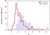 |
Fig. 3 Distribution of α for both models. |
Figure 4 shows the distribution of the dominant timescale, defined as τ = 1/(2πfb), where fb is the break frequency as determined by Eq. (2) for the bpl model.
 |
Fig. 4 Distribution of the dominant timescale for the bpl model. |
Although within several individual light curves we do observe sub–second variability, when the overall variance is dominated by a specific timescale, this mostly ranges between 0.2 and 30 s, with a logarithmic average of 4.1 s with a dispersion factor of 3.
3.3. Dominant timescale vs. duration
The 75 GRBs with a break frequency, or equivalently, with a dominant timescale τ, exhibit an interesting and unexpected property: τ is found to correlate with the overall duration expressed in terms of T90 (top panel of Fig. 5). Its significance is reliable: 7 × 10-15, 7 × 10-15, and 2 × 10-12 according to Pearson’s linear, Spearman’s, and Kendall’s coefficients, respectively. We modelled this relation with either a simple proportionality or with a power-law using the D’Agostini method (D’Agostini 2005) which naturally accounts for the extrinsic scatter (i.e. additional to the measurement uncertainties affecting each point). We conservatively assumed a 10% uncertainty on each value of T90. In the former case we obtained 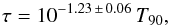 (3)with an extrinsic scatter σ(log τ) = 0.25 ± 0.05 (best-fitting parameter errors are given with 90% confidence throughout this section). Equivalently, on average the dominant timescale is about 20 times shorter than the overall duration, with a dispersion of nearly 0.3 dex. In the latter case, modelling with a power-law yields a slightly shallower dependence of τ on T90 than Eq. (3),
 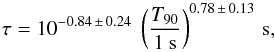 (4)with an extrinsic scatter σ(log τ) = 0.24 ± 0.04.
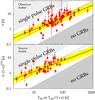 |
Fig. 5 Dominant timescale τ vs. duration T90 for the GRBs that are best fit with a bpl model in both the observer’s (top panel) and in the source rest frames (bottom panel). Solid and dashed lines show the best-fitting power-law and the best-fitting proportionality case, respectively. |
For 41 GRBs the redshift is known. For this subset we could study the analogous relation in the GRB source rest frame. The corresponding intrinsic quantities, denoted with subscript i, were calculated as follows: τi = τ/ (1 + z)0.6, which combines the cosmological dilation and the narrowing of pulses with energy as modelled by Fenimore et al. (1995); T90,i = T90/ (1 + z). In the latter case we did not apply the narrowing of pulses to the overall duration of the burst: this is correct especially in the presence of waiting times. The reason is that our sample of GRBs mostly consists of profiles with multiple pulses interspersed with waiting times. However, we verified that the results were not very sensitive to whether a = 0.6 or a = 1 is assumed, where the correction factor is parametrised as (1 + z)a. The bottom panel of Fig. 5 shows the result. The correlation is still significant: the p-values are 9 × 10⁻⁸, 1 × 10⁻⁶, and 8 × 10⁻⁷ according to Pearson’s linear, Spearman’s, and Kendall’s coefficients, respectively. Fitting the correlation with the same two models as in the observer’s frame case, we found almost identical values with larger uncertainties that are due to the lower number of points. 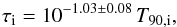 (5)with an extrinsic scatter σ(log τi) = 0.25 ± 0.07. Modelling this with a power-law, we obtain
 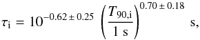 (6)with an extrinsic scatter σ(log τi) = 0.23 ± 0.05.
The average ratio between T90 and τ is higher than one order of magnitude. This rules out that the correlation has an obvious origin. Even for the few GRBs in our sample whose light curves consist of a single featureless pulse, no dominant timescale is identified. The reason is that the time interval chosen for the PDS calculation is not long enough to associate the break with the pulse duration itself that appears in the PDS so as to demand a bpl instead of pl. To illustrate why the two quantities are connected in no obvious way, Fig. 6 displays the time profile of 060117 as an example.
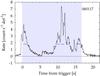 |
Fig. 6 Example of a light curve with a dominant timescale. This is the 15−150 keV profile of 060117, whose PDS is fit with bpl with τ = 1.0 s. Horizontal solid bars are as long as τ and emphasise the relevance of this timescale within the overall variability. The shaded area shows the T90 = 16.9–s interval. |
The top left region of the T90–τ space appears to be empty; we know it is populated by the obvious cases, such as that of a single smooth pulse, in which the only characteristic timescale is given by the pulse duration itself. Instead, the dearth of long-lasting GRBs with a short dominant timescale, such as T90/τ ≫ 1, has no explanation. To ensure that this is not an artefact of our procedure, we constructed a synthetic light curve by replicating and appending a real GRB profile with a short dominant timescale, so as to obtain an arbitrarily long GRB. As a result, our procedure did identify the same short dominant timescale within uncertainties, whereas the duration increased by construction. This fake GRB lay in the empty region. This rules out any selection bias in our procedure against this type of GRBs, and it raises the question as to why they are rarely seen. In conclusion, instead of a true correlation between τ and T90, the property that demands an explanation is the observed dearth of short-timescale-dominated long-T90 GRBs.
It might be wondered whether this holds for so-called ultra-long events (Levan et al. 2014; Gendre et al. 2013; Stratta et al. 2013; Virgili et al. 2013; Zhang et al. 2014; Boer et al. 2015). We therefore report our results on 130925A (Evans et al. 2014; Piro et al. 2014), although Swift-BAT data do not cover it in its entirety. Because of this, we did not include it in our selected sample from which the above ensemble properties have been drawn. In particular, the dominant timescale found by us, ~22 s (Table 1), was inevitably extracted from the first 103 s and is therefore not descriptive of the several-ks-long profile, so the issue remains unsettled.
In Fig. 3 of D16 we illustrated the difference between the two groups of PDS that are best fit with either bpl or pl and the meaning of dominant timescale, wherever one exists. In the most general case, the PDS concerns a light curve that is the result of superposing a number of pulses with different timescales. Whenever the total variance is mostly dominated by some specific timescale, this shows itself as the break in the PDS, which is best fit with bpl. Otherwise, when several different timescales have similar weights in the total variance, the resulting PDS exhibits no clear break and appears to be remarkably shallower (αpl ≲ 2) than that of individual pulses (αbpl> 2). If this interpretation is correct, profiles of GRBs with αpl ≲ 2 on average should have more pulses. This is indeed the case, as shown in Fig. 7.
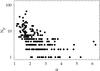 |
Fig. 7 Number of pulses as a function of the PDS slope α. GRBs that consist of a large number of pulses are more likely to exhibit a shallower PDS. |
3.4. PDS and peak energy Ep,i
We searched for possible relations between the properties of the PDS and intrinsic quantities of the prompt emission. In particular, from the sample with known redshift, we selected the GRBs with a well-constrained peak energy Ep,i of the time–averaged energy spectrum EF(E).
No correlation between Ep,i and τi was found for the subsample of GRBs with both observables. Conversely, we found a link between the PDS power-law index α for both models and Ep,i as shown in Fig. 8 (bottom panel), which displays the two quantities for a sample of 83 GRBs. Peak energy and redshift measures for this sample were taken from D16, where this correlation was studied in more detail with a larger data sample from several spacecraft. The power-law index of the PDS refers to the 15−150 keV light curve. On average, GRBs with higher peak energies exhibit lower PDS indexes. The p-values associated with Pearson’s, Spearman’s, and Kendall’s coefficients are 3.7 × 10⁻⁶, 3.9 × 10⁻⁷, and 8.6 × 10⁻⁷, respectively. These values do not account for the measurement uncertainties. Although these centroids are already the result of a scattering that is due to the individual uncertainties, we conservatively estimated their effect through MC simulations: we independently scattered each point assuming a log-normal distribution along Ep,i and using the marginal posterior distribution obtained for α for each GRB (Appendix A). We generated 1000 synthetic sets of 83 GRBs each and calculated the corresponding correlation coefficients. The 90% quantiles of the p-value distributions of the above-mentioned correlation coefficients are 3.5 × 10⁻⁴, 1.6 × 10⁻⁵, and 1.5 × 10⁻⁵, respectively. Hence, the significance of the correlation according to non–parametric tests lies in the range 10-5−10-4.
The top panel of Fig. 8 shows the same correlation in the observer frame for the same sample, where the observed peak energy Ep replaces Ep,i. This is useful to determine where Ep lies with respect to the BAT energy passband, in which light curves were extracted to evaluate its effect. Even considering only the GRBs whose Ep lies above the BAT passband, there are still a few cases for both models with α> 2. This rules out that the Ep,i–α correlation is the result of a bias connected with the energy band in which temporal profiles are extracted. In the observer plane, the correlation is slightly less significant: the same 90% quantiles are 4.2 × 10⁻⁴, 7.6 × 10⁻⁵, and 7.7 × 10⁻⁵, respectively. However, if the narrower range α< 4.5 is considered, the correlation is almost one order of magnitude more significant in the source rest frame than in the observer frame. The same property of a more significant correlation in the source rest frame than in the observer frame holds for the larger sample of D16.
We refer to D16 for an exhaustive analysis of the Ep,i − α correlation and its implications in the framework of different models proposed in the literature. As shown in D16, this correlation is found to hold and extend to GRBs detected with other current and past experiments with far better significance.
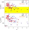 |
Fig. 8 Top panel: observed peak energy Ep vs. the power-law index α of the PDS (15−150 keV) for a sample of GRBs with known redshift and well-constrained time–averaged energy spectrum. The shaded area highlights the BAT energy passband. Bottom panel: same plot in the intrinsic plane, i.e. where the peak energy Ep,i refers to the GRB comoving frame. Circles (triangles) correspond to pl (bpl) model. Median errors are shown (top right). The dashed line shows the case α = 2. |
We studied the same relation for the PDS of each energy channel and show the result in Fig. 9.
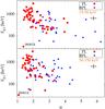 |
Fig. 9 Same as Fig. 8, except that α was obtained for each energy channel: 15−50 (top), and 50−150 keV (bottom). |
The same correlation seen in the total energy band is also evident in the individual energy channels with some notable differences, however. For the lower energy channel 15−50 keV, the correlation is even more significant than the full passband (3 × 10⁻⁷, 3 × 10⁻⁹, and 6 × 10⁻⁹ significance). Conversely, in the harder energy band the correlation is much weaker and more scattered (9 × 10⁻⁴, 2 × 10⁻⁴, and 1 × 10⁻⁴ significance).
More generally, if the sample is split into two subsets, depending on whether it is α< 2, the correlation is no more significant in each subset. This suggests that the correlation might mainly be due to the existence of two different classes of GRBs that are characterised by a shallow or a steep PDS.
To gain further insight, we performed some KS tests on the Ep,i distributions of the two classes: in the total energy band case we split the sample assuming α = 2 as the dividing line. The resulting p-value of a common Ep,i is 1.7 × 10⁻⁵ (5.9 × 10⁻⁶ when 060614 is excluded). Analogous tests on the samples of the two energy channels yield p-values of 4 × 10⁻⁶ and 6 × 10⁻³ for the 15−50 and the 50−150 keV band, respectively. Dropping 060614, these p-values decrease to 2 × 10⁻⁶ and 4 × 10⁻³. 060614 can be treated as an anomalous source for independent reasons: it shares properties with both long and short GRBs: its duration and its consistency with the Ep–Eiso favour the long classification (Amati et al. 2007); the negligible temporal lag of its initial spike, along with the significant absence of any typical SN associated to other long GRBs (Gehrels et al. 2006; Della Valle et al. 2006; Fynbo et al. 2006), and the possible evidence for an associated macronova (Yang et al. 2015; Kisaka et al. 2016; Jin et al. 2015), would place it in the short group, so that this GRB is still singular. See D16 for a thorough discussion of 060614.
That the dividing line is around α = 2 may hide a profound meaning in the theory of PDS formation (Titarchuk et al. 2007).
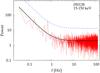 |
Fig. 10 PDS of 050128 in the 15−150 keV band. The solid (dashed) line shows the pl best–fitting model (3σ level above the continuum). |
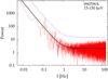 |
Fig. 11 PDS of 090709A in the 15−150 keV band. The solid (dashed) line shows the pl best–fitting model (3σ level above the continuum). |
3.5. Search for periodic signal
We searched the total and individual energy channel PDS of each GRB for periodic features above a 3σ (Gaussian) significance threshold and found none.
We then adopted an alternative approach: we split the 3 × T7σ interval into three equal sub–intervals, calculated the PDS for each, and averaged out the resulting PDS. We then minimised the log–likelihood of Eq. (A.7) with M = 3. The most obvious benefit of summing different PDS is a reduced statistical noise. Performing the search for periodic pulsations over these average PDS for each individual GRB in the total passband and in the two energy channels allowed us to pick up three GRBs with > 3σ significance. In the total passband 050128 (Fig. 10) and 090709A (Fig. 11) show a feature at f = 0.696 ± 0.035 Hz and at f = 0.123 ± 0.006 Hz, respectively. 070220 shows an excess in the 50−150 keV band at f = 0.321 ± 0.006 Hz (Fig. 12).
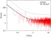 |
Fig. 12 PDS of 070220 in the 50−150 keV band. The solid (dashed) line shows the pl best–fitting model (3σ level above the continuum). |
The significance of each feature was determined by the p-value associated with the TR statistic in each case: the three corresponding p-values amount to 1.4 × 10⁻³, 2.3 × 10⁻³, and 2.6 × 10⁻³ for 050128, 090709A, and 070220, respectively. In units of Gaussian σ’s, they correspond to 3.2, 3.0, and 3.0. For 090709A similar searches gave analogous results (de Luca et al. 2010; Cenko et al. 2010). Because of the reasons explained in Appendix A, the significance accounts for the multi-trial search over the whole range of explored frequencies in each individual spectrum. The question we addressed instead concerns the probability that at least three GRBs out of 200 show features equal to or more significant than the observed ones by chance. To this aim, we took the smallest significance, that is, p = 1.4 × 10⁻³, as the success probability of a single trial. We used a binomial distribution with N = 200 trials and determined the probability of having n ≥ 3 successful events by chance, which is 0.2%. We might question whether this underestimates the true value. Instead, when we took the highest p-value as the success probability for the single trial, that is, p = 2.6 × 10⁻³, the resulting probability for the multi-trial was a mere 1%. Thus, the true value lies between 0.2 and 1%. This value does not allow us to make a strong statement about the evidence for coherent pulsations in some GRBs. However, there is a further, more subtle but nonetheless crucial caveat we did not mention so far, and which lies in the procedure with which we calculated the PDS for this search. Unlike for the previous parts of the present investigation, here we sliced the light curves into sub-intervals and averaged the PDS of each of them out. This is common practice for steady sources because it implicitly relies on the assumption of an ergodic process (e.g. Guidorzi 2011). While this is reasonable for a steady source, this is unlikely to be the case for the GRB signal. Therefore, in spite of the possible detection of coherent pulsation with ≲1% confidence, its interpretation is undermined by the implicit assumption of the GRB light curve thought of as an ergodic process, which can hardly make physical sense. We conclude that there is no unambiguous evidence for periodic features in this Swift-BAT GRB data set.
4. Summary and discussion
For the first time, a systematic analysis of individual PDS of long GRBs has been carried out using a statistical treatment that allowed us to properly model the continuum and search for possible periodic or QPOs in a self-consistent way. An analogous investigation based on the same technique was carried out by us (Dichiara et al. 2013b) on a sample of short GRBs, where we compared the derived distribution of the PDS slopes α with the preliminary one for a sample of long GRBs, finding no striking difference.
This technique, described in detail in Appendix A, has opened up the possibility to search for correlations between PDS and other key properties, the most significant and remarkable of which is Ep,i–α. In D16 we thoroughly studied this correlation over an enlarged sample of GRBs detected with different spacecraft and discussed its physical implications in the context of some prompt emission models. In particular, we linked the PDS slope to the relative strength of the fast component (timescale ≲ 1 s) in the light curve: when this is clearly present, the PDS is shallow (α ≲ 2) and shows no break. By contrast, when it is either weak or missing, the PDS is steeper (α> 2) with or without a break in the range 0.01−1 Hz. While a KS test between the T90 distributions of the two groups of PDS models reveals no difference (p-value of 65%), the bpl group on average possibly has fewer peaks/GRB (KS p-value of 7%), as also shown in Fig. 7 considering that they have higher αs than the pl group. Almost all of GRBs with N> 10 peaks have PDS slopes α< 2. This agrees with our interpretation of the PDS: GRBs with many peaks are more likely to cover a broader range of timescales, so that the resulting PDS is shallow and has no dominant timescale (see Fig. 3 in D16). The interpretation in terms of two independent components in GRB light curves is in accord with the results of previous investigations based on different techniques (Shen & Song 2003; Vetere et al. 2006; Gao et al. 2012).
As we discussed in D16, in the context of some of the GRB prompt emission models the observed variability tracks the intrinsic inner engine behaviour. If the engine is a newly formed black hole (BH) accreting from a disk, as predicted in the collapsar model (Woosley 1993; MacFadyen & Woosley 1999), it is interesting to compare our results with the PDS properties of other astrophysical sources that are known to be powered by accreting BHs. Specifically, accretion around BHs is known to be characterised by some scalings between BH mass, timescales, and accretion luminosity (relative to the Eddington limit). These scalings hold for Galactic stellar BHs (GBHs) and for super-massive BH (SMBH) that power active galactic nuclei (AGNs), according to the fundamental plane of BH activity (Merloni et al. 2003; Falcke et al. 2004). We took the sample of AGN PDS obtained by González-Martín & Vaughan (2012), who fit them either with a pl or with a so-called bending power-law, which differs from our bpl model only in the low-frequency regime, where power scales as f-1 instead of f0 for f ≪ fb. Our choice of f0 for GRBs is a consequence of the time finiteness of the GRB signal, which entails a constant power at f ≪ 1 /T, where T is the GRB duration. On the other hand, AGNs and GBHs are stationary sources that do not undergo irreversible processes like the sequence of events that make up the GRB phenomenon. As such, their red noise power extends to f ≪ 1 /T, where T is the duration of the observation window. This explains why f-1 is more appropriate for these sources than f0 at f ≪ 1 /T. We also considered the analogous distribution for a sample of magnetar bursts from Huppenkothen et al. (2013), who fitted the PDS with a similar and more general broken power-law model as an alternative to a simple pl. In terms of stochastic processes, the magnetar burst sample is more similar to that of GRBs because of the non-stationary character and even shorter duration.
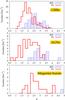 |
Fig. 13 Distribution of the PDS slope for both models (solid is pl, filled is bpl) for three classes of astrophysical sources: GRBs (top, this work), AGNs (middle, from González-Martín & Vaughan 2012), and magnetar bursts (bottom, from Huppenkothen et al. 2013). |
Figure 13 shows the comparison between the PDS slope distribution of our GRB set, that of AGNs, and that of magnetar outbursts. Although all of the distributions span very similar ranges, the distributions that appear more alike are those of GRBs and AGNs: the distributions for both models look remarkably similar, at least as far as their respective ranges are concerned.
Furthermore, analogous trends with the photon energy are observed: PDS are shallower for harder energy channels, as observed for AGNs (González-Martín & Vaughan 2012), for GBHs (Nowak et al. 1999), and for the average PDS of GRBs (Beloborodov et al. 2000; Guidorzi et al. 2012; Dichiara et al. 2013a). PDS of GBHs are generally more complicated and strongly depend on the source state: in the soft state, they are typically modelled with a bending pl with a high-frequency index α> 2, whereas α can vary in the range between 1 and 2 (Cui et al. 1997; Nowak et al. 1999; Remillard & McClintock 2006). By contrast, unlike for GRBs, some AGN and GBH PDS are also characterised by QPOs. Evidence for QPOs has recently been found in the PDS of a few magnetar bursts (Huppenkothen et al. 2014a,b).
Concerning the dominant timescales τ identified in the PDS, we found no correlation between τ and other intrinsic properties, such as Ep,i, or Eiso. In the AGN case, the timescale corresponding to the break frequency is known to scale with the BH mass (e.g., Markowitz et al. 2003). In GRBs the origin of dominant timescales is likely different: on average, most low-Ep,i GRBs, which also have correspondingly low peak luminosities, have a several-second-long dominant timescale and either weak or absent subsecond variability, as indicated by the Ep,i–α correlation (Figs. 8 and 9; see also D16). Assuming the BH scaling, we would infer higher masses for these GRBs than for the bulk of GRBs. However, they look like they can hardly be associated with the most massive BHs among the possible GRB progenitor candidates, given their lower luminosities.
Overall, we have to be cautious in building upon these analogies between GRBs and AGNs purely based on the PDS slopes, firstly because of the strong non-stationary character of GRBs, secondly because the BH nature of GRB inner engines is not yet established beyond doubt. Nonetheless, regardless of the origin of GRB variability (see D16), the result illustrated in Fig. 13 might stem from a common process that rules accreting BH across different mass scales.
Concerning the presence of dominant timescales, an unexpected result from our analysis is the absence or dearth of subsecond-dominant timescales (τ ≲ 1 s) in long GRBs (T90 ≳ 10–20 s in the rest frame; see bottom panel of Fig. 5). To our knowledge, this type of constraint for long GRBs is not predicted in any prompt emission model that appeared thus far in the literature. We showed that this dearth is a genuine property of real light curves and not an artefact of our technique. In other words, when short-timescale variability dominates the light-curve variance, the overall duration of the prompt emission cannot last longer than a few tens of seconds. Equivalently, very long GRBs cannot have dominant timescales as short as τ ≲ 1 s, that is, a significant fraction of the temporal power must lie in the slow (> 1 s) component. This unexpected constraint between short-timescale variability and overall duration of GRBs should be taken into account in prompt emission models.
Although we found three GRBs with some evidence (~3σ significance) for coherent pulsations, the overall multi-trial probability that these are mere statistical flukes is about 1%, that is, not negligible. The overall lack of unambiguous evidence for periodic signal in GRB prompt light curves does not clash with models in which the GRB progenitor injects energy following a periodic or quasi-periodic pattern, such as in the newly born millisecond magnetar model (Usov 1992; Thompson et al. 2004; Metzger et al. 2011), or due to the viscous spindown of a BH (van Putten & Gupta 2009). The reason is that a localised release of a comparable amount of energy entails the formation of an e± and gamma-ray fireball (Cavallo & Rees 1978), which may quench the imprinted temporal pattern, unlike what occurs for the possibly associated gravitational-wave signal (van Putten 2009). Our conclusion assumes that all GRBs are different realisations of a common stochastic process. If we drop this assumption, we cannot exclude that the periodic patterns observed in these three GRBs are real (Zhang et al. 2016) and that for some unknown reasons they are intrinsically different from the bulk of GRBs.
The LRT based on the posterior predictive distribution naturally accounts for the dependence of the posterior distribution over the whole parameter space; however, unlike for the Bayes factor, this is true only for the simpler model pl and not for the more complex bpl. This means that while its usage is reliable in excluding the simpler hypothesis of pl, this is not necessarily evidence for bpl. The case for bpl as a plausible alternative to pl is supported by independent reasons discussed in Sect. A.1.1 (Appendix A), however.
Acknowledgments
We are grateful to the anonymous referee for insighful comments that improved the paper, and to Filippo Frontera, Lev Titarchuk, and Chris Koen for useful discussions. We acknowledge support by PRIN MIUR project on “Gamma Ray Bursts: from progenitors to physics of the prompt emission process”, P. I. F. Frontera (Prot. 2009 ERC3HT).
References
- Amati, L., Frontera, F., Tavani, M., et al. 2002, A&A, 390, 81 [NASA ADS] [CrossRef] [EDP Sciences] [Google Scholar]
- Amati, L., Della Valle, M., Frontera, F., et al. 2007, A&A, 463, 913 [NASA ADS] [CrossRef] [EDP Sciences] [Google Scholar]
- Anderson, T. W., & Darling, D. A. 1952, Ann. Math. Stat., 23, 193 [CrossRef] [Google Scholar]
- Baldeschi, A., & Guidorzi, C. 2015, A&A, 573, L7 [NASA ADS] [CrossRef] [EDP Sciences] [Google Scholar]
- Barret, D., & Vaughan, S. 2012, ApJ, 746, 131 [NASA ADS] [CrossRef] [Google Scholar]
- Barthelmy, S. D., Barbier, L. M., Cummings, J. R., et al. 2005, Space Sci. Rev., 120, 143 [NASA ADS] [CrossRef] [Google Scholar]
- Belli, B. M. 1992, ApJ, 393, 266 [NASA ADS] [CrossRef] [Google Scholar]
- Beloborodov, A. M. 2010, MNRAS, 407, 1033 [NASA ADS] [CrossRef] [Google Scholar]
- Beloborodov, A. M., Stern, B. E., & Svensson, R. 1998, ApJ, 508, L25 [NASA ADS] [CrossRef] [Google Scholar]
- Beloborodov, A. M., Stern, B. E., & Svensson, R. 2000, ApJ, 535, 158 [NASA ADS] [CrossRef] [Google Scholar]
- Beniamini, P., & Granot, J. 2015, MNRAS submitted, [arXiv:1509.02192] [Google Scholar]
- Boer, M., Gendre, B., & Stratta, G. 2015, ApJ, 800, 16 [NASA ADS] [CrossRef] [Google Scholar]
- Cavallo, G., & Rees, M. J. 1978, MNRAS, 183, 359 [NASA ADS] [CrossRef] [Google Scholar]
- Cenko, S. B., Butler, N. R., Ofek, E. O., et al. 2010, AJ, 140, 224 [NASA ADS] [CrossRef] [Google Scholar]
- Cui, W., Zhang, S. N., Focke, W., & Swank, J. H. 1997, ApJ, 484, 383 [NASA ADS] [CrossRef] [Google Scholar]
- D’Agostini, G. 2005, ArXiv e-prints [arXiv:physics/0511182] [Google Scholar]
- de Luca, A., Esposito, P., Israel, G. L., et al. 2010, MNRAS, 402, 1870 [NASA ADS] [CrossRef] [Google Scholar]
- Della Valle, M., Chincarini, G., Panagia, N., et al. 2006, Nature, 444, 1050 [NASA ADS] [CrossRef] [PubMed] [Google Scholar]
- Derishev, E. V., Kocharovsky, V. V., & Kocharovsky, V. V. 1999, ApJ, 521, 640 [NASA ADS] [CrossRef] [Google Scholar]
- Dichiara, S., Guidorzi, C., Amati, L., & Frontera, F. 2013a, MNRAS, 431, 3608 [NASA ADS] [CrossRef] [Google Scholar]
- Dichiara, S., Guidorzi, C., Frontera, F., & Amati, L. 2013b, ApJ, 777, 132 [NASA ADS] [CrossRef] [Google Scholar]
- Dichiara, S., Guidorzi, C., Amati, L., Frontera, F., & Margutti, R. 2016, A&A, 589, A97 (D16) [NASA ADS] [CrossRef] [EDP Sciences] [Google Scholar]
- Evans, P. A., Willingale, R., Osborne, J. P., et al. 2014, MNRAS, 444, 250 [NASA ADS] [CrossRef] [Google Scholar]
- Falcke, H., Körding, E., & Markoff, S. 2004, A&A, 414, 895 [NASA ADS] [CrossRef] [EDP Sciences] [Google Scholar]
- Fenimore, E. E., in ’t Zand, J. J. M., Norris, J. P., Bonnell, J. T., & Nemiroff, R. J. 1995, ApJ, 448, L101 [NASA ADS] [CrossRef] [Google Scholar]
- Frontera, F., & Fuligni, F. 1979, ApJ, 232, 590 [NASA ADS] [CrossRef] [Google Scholar]
- Fynbo, J. P. U., Watson, D., Thöne, C. C., et al. 2006, Nature, 444, 1047 [NASA ADS] [CrossRef] [PubMed] [Google Scholar]
- Gao, H., Zhang, B.-B., & Zhang, B. 2012, ApJ, 748, 134 [NASA ADS] [CrossRef] [Google Scholar]
- Gehrels, N., Chincarini, G., Giommi, P., et al. 2004, ApJ, 611, 1005 [NASA ADS] [CrossRef] [Google Scholar]
- Gehrels, N., Norris, J. P., Barthelmy, S. D., et al. 2006, Nature, 444, 1044 [NASA ADS] [CrossRef] [PubMed] [Google Scholar]
- Gendre, B., Stratta, G., Atteia, J. L., et al. 2013, ApJ, 766, 30 [NASA ADS] [CrossRef] [Google Scholar]
- Giannios, D. 2008, A&A, 480, 305 [NASA ADS] [CrossRef] [EDP Sciences] [Google Scholar]
- Giannios, D. 2012, MNRAS, 422, 3092 [NASA ADS] [CrossRef] [Google Scholar]
- González-Martín, O., & Vaughan, S. 2012, A&A, 544, A80 [NASA ADS] [CrossRef] [EDP Sciences] [Google Scholar]
- Groth, E. J. 1975, ApJ, 29, 285 [Google Scholar]
- Guidorzi, C. 2011, MNRAS, 415, 3561 [NASA ADS] [CrossRef] [Google Scholar]
- Guidorzi, C. 2015, Astronomy and Computing, 10, 54 [Google Scholar]
- Guidorzi, C., Margutti, R., Amati, L., et al. 2012, MNRAS, 422, 1785 [NASA ADS] [CrossRef] [Google Scholar]
- Hjorth, J. 2013, Phil. Trans. Roy. Soc. London Ser. A, 371, 20275 [Google Scholar]
- Hjorth, J., Malesani, D., Jakobsson, P., et al. 2012, ApJ, 756, 187 [NASA ADS] [CrossRef] [Google Scholar]
- Huppenkothen, D., Watts, A. L., Uttley, P., et al. 2013, ApJ, 768, 87 [NASA ADS] [CrossRef] [Google Scholar]
- Huppenkothen, D., D’Angelo, C., Watts, A. L., et al. 2014a, ApJ, 787, 128 [NASA ADS] [CrossRef] [Google Scholar]
- Huppenkothen, D., Heil, L. M., Watts, A. L., & Göğüş, E. 2014b, ApJ, 795, 114 [NASA ADS] [CrossRef] [Google Scholar]
- Israel, G. L., & Stella, L. 1996, ApJ, 468, 369 [NASA ADS] [CrossRef] [Google Scholar]
- Jin, Z.-P., Li, X., Cano, Z., et al. 2015, ApJ, 811, L22 [NASA ADS] [CrossRef] [Google Scholar]
- Kass, R. E., & Raftery, A. 1995, J. Am. Stat. Assoc., 90, 773 [Google Scholar]
- Kisaka, S., Ioka, K., & Nakar, E. 2016, ApJ, 818, 104 [NASA ADS] [CrossRef] [Google Scholar]
- Lazzati, D. 2002, MNRAS, 337, 1426 [NASA ADS] [CrossRef] [Google Scholar]
- Leahy, D. A., Darbro, W., Elsner, R. F., et al. 1983, ApJ, 266, 160 [NASA ADS] [CrossRef] [Google Scholar]
- Levan, A. J., Tanvir, N. R., Starling, R. L. C., et al. 2014, ApJ, 781, 13 [NASA ADS] [CrossRef] [Google Scholar]
- Lyutikov, M., & Blandford, R. 2003, ArXiv e-prints [arXiv:astro-ph/0312347] [Google Scholar]
- MacFadyen, A. I., & Woosley, S. E. 1999, ApJ, 524, 262 [NASA ADS] [CrossRef] [Google Scholar]
- Markowitz, A., Edelson, R., Vaughan, S., et al. 2003, ApJ, 593, 96 [NASA ADS] [CrossRef] [Google Scholar]
- Merloni, A., Heinz, S., & di Matteo, T. 2003, MNRAS, 345, 1057 [NASA ADS] [CrossRef] [Google Scholar]
- Mészáros, P., & Rees, M. J. 2011, ApJ, 733, L40 [NASA ADS] [CrossRef] [Google Scholar]
- Metzger, B. D., Giannios, D., Thompson, T. A., Bucciantini, N., & Quataert, E. 2011, MNRAS, 413, 2031 [NASA ADS] [CrossRef] [Google Scholar]
- Narayan, R., Paczynski, B., & Piran, T. 1992, ApJ, 395, L83 [NASA ADS] [CrossRef] [Google Scholar]
- Norris, J. P., & Bonnell, J. T. 2006, ApJ, 643, 266 [NASA ADS] [CrossRef] [Google Scholar]
- Norris, J. P., Nemiroff, R. J., Bonnell, J. T., et al. 1996, ApJ, 459, 393 [NASA ADS] [CrossRef] [Google Scholar]
- Nowak, M. A., Vaughan, B. A., Wilms, J., Dove, J. B., & Begelman, M. C. 1999, ApJ, 510, 874 [NASA ADS] [CrossRef] [Google Scholar]
- Papoulis, A., & Pillai, S. U. 2002, Probability, Random Variables, and Stochastic Processes, Fourth Edition (McGraw-Hill Higher Education) [Google Scholar]
- Pe’er, A., Mészáros, P., & Rees, M. J. 2006, ApJ, 642, 995 [NASA ADS] [CrossRef] [Google Scholar]
- Piro, L., Troja, E., Gendre, B., et al. 2014, ApJ, 790, L15 [NASA ADS] [CrossRef] [Google Scholar]
- Rees, M. J., & Meszaros, P. 1994, ApJ, 430, L93 [NASA ADS] [CrossRef] [Google Scholar]
- Rees, M. J., & Mészáros, P. 2005, ApJ, 628, 847 [NASA ADS] [CrossRef] [Google Scholar]
- Remillard, R. A., & McClintock, J. E. 2006, ARA&A, 44, 49 [NASA ADS] [CrossRef] [Google Scholar]
- Rizzuto, D., Guidorzi, C., Romano, P., et al. 2007, MNRAS, 379, 619 [NASA ADS] [CrossRef] [Google Scholar]
- Rossi, E. M., Beloborodov, A. M., & Rees, M. J. 2006, MNRAS, 369, 1797 [NASA ADS] [CrossRef] [Google Scholar]
- Ryde, F., Borgonovo, L., Larsson, S., et al. 2003, A&A, 411, L331 [NASA ADS] [CrossRef] [EDP Sciences] [Google Scholar]
- Sakamoto, T., Barthelmy, S. D., Baumgartner, W. H., et al. 2011, ApJS, 195, 2 [NASA ADS] [CrossRef] [Google Scholar]
- Shen, R.-F., & Song, L.-M. 2003, PASJ, 55, 345 [NASA ADS] [CrossRef] [Google Scholar]
- Stratta, G., Gendre, B., Atteia, J. L., et al. 2013, ApJ, 779, 66 [NASA ADS] [CrossRef] [Google Scholar]
- Thompson, T. A., Chang, P., & Quataert, E. 2004, ApJ, 611, 380 [NASA ADS] [CrossRef] [Google Scholar]
- Thompson, C., Mészáros, P., & Rees, M. J. 2007, ApJ, 666, 1012 [NASA ADS] [CrossRef] [Google Scholar]
- Titarchuk, L., Shaposhnikov, N., & Arefiev, V. 2007, ApJ, 660, 556 [NASA ADS] [CrossRef] [Google Scholar]
- Titarchuk, L., Farinelli, R., Frontera, F., & Amati, L. 2012, ApJ, 752, 116 [NASA ADS] [CrossRef] [Google Scholar]
- Usov, V. V. 1992, Nature, 357, 472 [NASA ADS] [CrossRef] [Google Scholar]
- van der Klis, M. 1989, in Timing Neutron Stars, eds. H. Ögelman, & E. P. J. van den Heuvel (Dordrecht: Kluwer), 27 [Google Scholar]
- van Putten, M. H. P. M. 2009, MNRAS, 396, L81 [NASA ADS] [CrossRef] [Google Scholar]
- van Putten, M. H. P. M., & Gupta, A. C. 2009, MNRAS, 394, 2238 [NASA ADS] [CrossRef] [Google Scholar]
- Vaughan, S. 2010, MNRAS, 402, 307 [NASA ADS] [CrossRef] [Google Scholar]
- Vaughan, S. 2013, Roy. Soc. London Philos. Trans. Ser. A, 371, 20110549 [Google Scholar]
- Vetere, L., Massaro, E., Costa, E., Soffitta, P., & Ventura, G. 2006, A&A, 447, 499 [NASA ADS] [CrossRef] [EDP Sciences] [Google Scholar]
- Virgili, F. J., Mundell, C. G., Pal’shin, V., et al. 2013, ApJ, 778, 54 [NASA ADS] [CrossRef] [Google Scholar]
- Woosley, S. E. 1993, ApJ, 405, 273 [NASA ADS] [CrossRef] [Google Scholar]
- Woosley, S. E., & Bloom, J. S. 2006, ARAA, 44, 507 [NASA ADS] [CrossRef] [Google Scholar]
- Yang, B., Jin, Z.-P., Li, X., et al. 2015, Nat. Comms., 6, 7323 [Google Scholar]
- Zhang, B., & Yan, H. 2011, ApJ, 726, 90 [NASA ADS] [CrossRef] [Google Scholar]
- Zhang, B.-B., Zhang, B., Murase, K., Connaughton, V., & Briggs, M. S. 2014, ApJ, 787, 66 [NASA ADS] [CrossRef] [Google Scholar]
- Zhang, B. B., Zhang, B., & Castro-Tirado, A. J. 2016, ApJ, 820, L32 [NASA ADS] [CrossRef] [Google Scholar]
Appendix A: PDS modelling
We start from the general assumption that a time series is the outcome of a stochastic process. A broad class of processes is the result of a linear system that operates linearly on an input process x(t) and yields another stochastic process y(t) = L [ x(t) ]. One example is given by the shot noise, which results from an input z(t) of Poisson impulses, 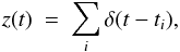 (A.1)where ti are Poisson points along the time axis with a given average rate λ, and the output shot noise process is
 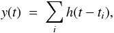 (A.2)where h(t) is a given deterministic function of time, so that the linear operator is in this example the convolution with the chosen deterministic function, y = h ∗ z. The expected PDS Syy(ω) of y(t) at ω> 0 is given by
 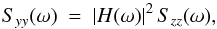 (A.3)where Szz(ω) is the PDS of the Poisson process, so it is ruled by the characteristic
  white-noise distribution, and | H(ω) | 2 is the square modulus of the Fourier transform of the deterministic function acting like a scaling factor at any given frequency. From Eq. (A.3) the PDS of the output process inherits the same distribution, where the expected power at ω is | H(ω) | 2 (Israel & Stella 1996). We can complicate this further, for example, by considering shot noise derived from a generalised Poisson process4, in which the input process is given by an impulse train with variable intensity, which can be itself another random variable ci:
 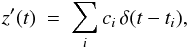 (A.4)and/or consider a Poisson process with variable rate λ(t) (e.g. for the study of shot noise in the PDS of solar X-ray flares, Frontera & Fuligni 1979) and/or the combination of different deterministic functions. Therefore, for this type of processes the coloured part of the PDS is mostly determined by the shape of the average deterministic profile that is convolved with the point process, with possible contribution from ci when this is characterised by correlated noise as well.
These processes yield a satisfactory description of the observed PDS of many astrophysical time series that can be treated as stationary (or, at least, locally stationary) processes, where the deterministic function h(t) describes the shape of a single shot. Our procedure assumes that GRB time profiles can be described by a process obtained by convolving the typical shape h(t) of an individual pulse with a generalised Poisson process like that of Eq. (A.4). At first glance, this assumption appears to be plausible for both the deterministic and the stochastic sides of the process: a typical pulse shape has indeed been identified in the form of a fast-rise exponential decay (FRED; Norris et al. 1996); the sequence of pulses, treated as a point process, is compatible with a Poisson process as long as long quiescent times are neglected (Baldeschi & Guidorzi 2015). In Sect. A.1 we discuss the shortcomings of this assumption and implications on the results.
For sums of independent PDS, the power in each frequency bin distributes like a , where the degrees of freedom, 2 M, is given by two times M, that is, the number of original spectra that are summed (van der Klis 1989). Let Pj be the observed power at frequency bin j and Sj its model value. The corresponding probability density function for Pj given the expected value Sj is given by 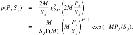 (A.5)where Γ() is the gamma function.
The joint likelihood function, p(P | S,H), for a given PDS P = { P1,P2,...,PN/ 2−1 }, given a generic model H with expected values S = { S1,S2,...,SN/ 2−1 }, is given by 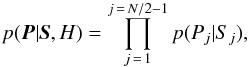 (A.6)where N is the number of bins in the light curves. We excluded the Nyquist frequency bin (j = N/ 2), since this follows a different distribution,
  (van der Klis 1989).
Maximising Eq.(A.6) is equivalent to minimising the corresponding un–normalised negative log–likelihood, L(P,S,H),  (A.7)So far, the dependence of the joint log–likelihood in Eq. (A.7) on model H is implicit through the model values, Sj (see also Barret & Vaughan 2012).
We determine the best–fitting model and the relative best–fitting parameters in the Bayesian context. From the Bayes theorem, the posterior probability density function of the parameters of a given model H and for a given observed PDS P is  (A.8)where the first term in the numerator of the right-hand side of Eq. (A.8) is the likelihood function of Eq. (A.6), p(S,H) is the prior distribution of the model parameters, in addition to the normalising term at the denominator.
We assumed uninformative prior distributions, except for the white-noise level, for which we used a conservative Gaussian centred on the pure Poissonian value of 2 with σ = 0.2 (Sect. 3.1). For the normalisation term N we adopted Jeffrey’s prior (see V10) given that it spans several decades, whereas a flat prior was used for the remaining parameters. The question of uninformative priors is the matter of on-going research in statistics, and the choice could depend on the specific problem. Finding the mode of the posterior probability of Eq. (A.8) is therefore equivalent to minimising the negative log–likelihood (A.7).
For each PDS we adopted the following fitting procedure. First, we tried to fit the PDS with a simple pl model described by Eq. (1) where the free parameters are the normalisation constant N, the power-law index α (> 0), and the white-noise level B. The logarithm of the normalisation was used instead of N itself because its posterior is more symmetric and easier to handle.
For a sizable part of our sample the PDS required the more complex model described by bpl (Eq. (2)). The reasons for the choice of this particular model are explained in Sect. 2.3.
We adopted the Bayesian procedure presented by V10 for estimating the posterior density of the model parameters through a Markov chain Monte Carlo (MCMC) algorithm such as the random–walk Metropolis–Hastings in the implementation of the R package MHadaptive5 (v.1.1-2). V10 treated the case M = 1, whereas we considered a more general M ≥ 1. We started by approximating the posterior using a multivariate normal distribution centred on the mode and whose covariance matrix is that obtained by minimisation of Eq. (A.7). For a given PDS, we generated 5.1 × 10⁴ sets of simulated parameters and retained one every five MCMC iterations after excluding the first 1000. The remaining 104 sets of parameters were therefore used to approximate the posterior density. To check the quality of the fit results and search for interesting features, such as QPO or periodic signatures superposed to the continuum spectrum, we used each set of simulated parameters of the PDS model to generate as many synthetic PDS from the posterior predictive distribution. Hence for a given observed PDS, this procedure allowed us to directly calculate 104 simulated PDS and use them to infer the probability density function of all the statistics we are interested in.
Let Ŝj be the model value at frequency bin j obtained with the best-fit parameters at the mode of the posterior. Following V10, we define the following quantity, Rj = 2MPj/Ŝj. If the true model Sj were known, Rj would be exactly -distributed. However, estimating it through Ŝj affects its distribution. The advantage of using the posterior predictive distribution is that no assumption on the nature of the distribution of Rj is required when we need to determine the corresponding p-values, since its probability density function (hereafter pdf) is sampled through the simulated spectra and the uncertainties in the model are automatically included. Let  be the jth bin power of the kth simulated PDS. Correspondingly, we also define
  . We chose three different statistics:
-
 (k = 1,...,104). This statistic picks up the maximum deviation from the continuum spectrum for each simulated PDS. The observed value TR = maxj(2MPj/Ŝj) is then compared with the simulated distribution and the significance is evaluated directly. By construction, it implicitly accounts for the multitrial search performed all over the frequencies.
 -
Ak is the Anderson–Darling (AD) statistic (Anderson & Darling 1952) obtained for the kth set of
 compared with a distribution.
 -
Analogously, KSk is the Kolmogorov–Smirnov (KS) statistic obtained for the kth set of
compared with a distribution.
For each of the three statistics, comparing the values obtained from the observed PDS with the corresponding distribution of simulated values immediately yields the significance of possible deviations such as that of a QPO, or the goodness of the fit, as indicated by the AD and KS statistics. As in G12, in addition to the KS, we chose the AD statistic because it is sensitive to a few outliers from the expected distribution.
For each GRB the choice between the two competing models was determined by the likelihood ratio test (LRT) in the Bayesian implementation described by V10. As for the aforementioned statistics, from the posterior predictive distribution we sampled the pdf of the TLRT statistic defined as ![Mathematical equation: \appendix \setcounter{section}{1} \begin{eqnarray} \label{eq:T_LRT} T_{\rm LRT} &=& -\log{\frac{p(\vec{P}|{\vec{\hat{S}}_{\rm PL}}, {\rm PL})}{p(\vec{P}|{\vec{\hat{S}}_{\rm BPL}}, {\rm BPL})}}\nonumber\\[3mm] &=& L(\vec{P},{\vec{\hat{S}}_{\rm PL}},{\rm PL}) - L(\vec{P},{\vec{\hat{S}}_{\rm BPL}},{\rm BPL}), \end{eqnarray}](/articles/aa/full_html/2016/05/aa27642-15/aa27642-15-eq436.png) (A.9)where ŜH denotes the model obtained with the parameters at the mode of the posterior distribution of a generic model H. The statistics in Eq. (A.9) is then sampled using the simulated PDS
(A.9)where ŜH denotes the model obtained with the parameters at the mode of the posterior distribution of a generic model H. The statistics in Eq. (A.9) is then sampled using the simulated PDS  (k = 1,...,104) and compared with the observed value. For the LRT test, we performed 103 simulations and accepted the bpl model when the probability of chance improvement was lower than 1% (see Sect. 2.3). As remarked in Sect. 2.3, while this type of LRT accounts for the whole parameter space of the simpler model, the same does not hold for the alternative one, as is the case when we use the Bayes factor. Consequently, the rejection of pl does not necessarily imply that bpl is a better option. However, for the limited scope of this investigation, on independent grounds bpl represents a sensible alternative (Sect. A.1.1).
Finally, after we determined the best–fitting model, we sampled through the MCMC simulation the joint posterior distribution of the model parameters and provided mean and standard deviation for each of them. As an example, Fig. A.1 shows the marginal posterior distributions of all the pairs of parameters of the bpl model for 050713A.
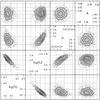 |
Fig. A.1 Example of marginal posterior distributions for the pairs of parameters of the bpl model obtained from 104 simulated posterior simulations for 050713A (only 2000 points are shown for clarity). Solid lines show the contour levels. |
The goodness of fit is established by the p-values associated to the AD and KS statistics. In addition, we also compare the distribution of Rj of the observed PDS against the expected distribution, as shown in Fig. A.2 for 050713A.
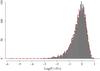 |
Fig. A.2 Distribution of log (Pj/Ŝj) for 050713A (Fig. 1). The dashed line shows the relative renormalised |
Appendix A.1: Shortcomings of the procedure and implications
The procedure relies on the assumption that GRB light curves can be described by stochastic processes resulting from the convolution of deterministic pulse shape with Poisson point processes. However, this is challenged by the short-lived and non-stationary nature of GRBs. Specifically, the following assumed properties somehow come into question:
-
1.
Are the pl and bpl models appropriate to GRBs?
-
2.
Is the unbinned power distributed around the model according to
? -
3.
Is the power at different frequency bins distributed in an uncorrelated way?
Appendix A.1.1: Are the PDS models appropriate?
Assuming a rough and simplistic pulse shape such as that of a simple exponential with a negligible rise time, h(t) = U(t) e− t/τ, where U(t) is the step function (1 at t> 0, 0 otherwise), the expected PDS is calculated in a straightforward way,  (A.10)which is included in our bpl model for α = 2 and νb = (2 πτ)-1. This description was adopted in the past to estimate the characteristic time of a typical shot in GRBs (Belli 1992) and in solar X-ray flares (Frontera & Fuligni 1979). Accounting for more realistic pulse-shape profiles yields complicated, wobbling PDS with a broad range of slopes at high frequencies (Lazzati 2002). This justifies the choice of a general shape like that of bpl, whereas the pl is given by the superposition of multiple shots with a range of different characteristic times as described in Sect. 3.3 and illustrated by D16. An even more general model was succesfully adopted for the PDS of magnetar outbursts (Huppenkothen et al. 2013).
Appendix A.1.2: Is the power  -distributed?
We start by considering the results of previous investigations that focused on the average PDS of a sample of GRBs and on how the power is distributed around it at each given frequency. While the distribution also depends on the adopted normalisation between different GRBs, the hypothesis was found to be acceptable for a peak-count-rate-normalised sample of BATSE GRBs (Beloborodov et al. 1998) and for a net-variance-normalised sample of Swift-BAT GRBs (Guidorzi et al. 2012). The assumption of a GRB as a stochastic process like that of a generalised shot noise convolved with one or more deterministic pulse shapes provides a theoretical justification for the distribution of power. However, in practice the sequence of pulses making up one GRB is limited, and only a few pulses are often observed. As a consequence, the PDS is dominated by the deterministic structure of the few shots (in addition to the uncorrelated noise that is due to the counting statistics) instead of the stochastic character brought in by the random point process. In this limit, the power is therefore seen to fluctuate significantly less than what we would expect from a . This is more evident in the low-frequency bins, where the signal power dominates the white-noise level (Huppenkothen et al. 2013). This is best illustrated by the limiting case of a single pulse, in which the PDS can be seen as the combination of a deterministic signal plus uncorrelated noise that is due to counting statistics: in the Leahy normalisation the power is distributed according to a non-central  , where Ps is the expected signal power (Groth 1975; Guidorzi 2011).
This complication is connected with the degeneracy of the problem: we can hardly identify what is due to a deterministic (typically unknown) signal as opposed to what is due to undersampling (because of the finiteness of the signal itself) of the stochastic side of the process. This directly brings us to the next question.
Appendix A.1.3: Is the PDS autocorrelated?
In the ideal case of a sufficiently long sequence of pulses, the resulting PDS -oscillates around the average expected PDS of the deterministic pulses. The PDS of a single pulse can be seen as single realisation of the process, where the power in each frequency bin is a single realisation of a -distributed variable, whose expected value is given by the model. However, as noted in the previous section, the PDS of a single pulse fluctuates around the deterministic model of that specific pulse less than a at low frequencies. Both properties combined imply that the PDS of a single pulse presents some degree of autocorrelation: as an example, if the power lies below the model at a given low frequency where the signal power is much greater than white noise, then a number of adjacent bins will lie below the model values as well. This undermines the assumption of independence between different frequency bins upon which the joint likelihood of Eq. (A.6) is based.
In the attempt of evaluating the effect of this problem on the results, it is worth noting that only the relatively few low-frequency bins are affected. On the other hand, this is precisely the frequency range where the comparison between the two competing models mostly matters. In addition, it is reassuring that the preference for bpl over pl, as established by a likelihood that overestimates the null-hypothesis variance, works conservatively so that bpl cannot be mistakenly preferred and is better a fortiori. As an illustrative case, we show the PDS of 140209A (Fig. A.3), which has the lowest p-value of the best-fit models of all our samples (Sect. 3). The quality of the fit is very poor, as assessed by the compatibility with the assumption that the PDS oscillates around the model as a . However, although the uncertainties on the best-fit parameters are to be taken with caution, the overall shape of the PDS is clearly very well described by the preferred model (bpl in this case).
To summarise, we conclude that despite the problems at low-frequencies, the assumptions upon which our procedure relies are acceptable and the breakdown of the statistical independence of the power at low frequencies does not alter its conservative character as for the preference for the more complicate model of bpl over the simple pl.
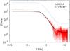 |
Fig. A.3 PDS and best-fit model of 140209A, the GRB with the lowest p-value of the preferred model (a bpl). The poor quality is mainly due to the low-frequency correlated power, which oscillates less than a |
All Tables
Best–fitting model along with means and standard deviations of the parameters’ posterior distributions for each GRB of the sample of 215 events in the total 15−150 keV energy band.
Best–fitting model along with means and standard deviations of the parameters’ posterior distributions for each GRB of the sample of 215 events in the 15−50 keV energy band.
Best–fitting model along with means and standard deviations of the parameters’ posterior distributions for each GRB of the sample of 215 events in the 50−150 keV energy band.
All Figures
|
Fig. 1 Examples of individual PDS. Dashed lines show the corresponding best–fitting model. Dotted lines show the 3σ threshold for periodic pulsations. Top: the PDS of 110119A can be fitted with a simple pl model and background. Bottom: fitting the PDS of 050713A significantly improves with a bpl model. |
| In the text | |
|
Fig. 2 Distribution of the white-noise level B. The vertical dashed line shows the pure Poissonian case. The solid Gaussian shows the prior distribution on B. |
| In the text | |
|
Fig. 3 Distribution of α for both models. |
| In the text | |
|
Fig. 4 Distribution of the dominant timescale for the bpl model. |
| In the text | |
|
Fig. 5 Dominant timescale τ vs. duration T90 for the GRBs that are best fit with a bpl model in both the observer’s (top panel) and in the source rest frames (bottom panel). Solid and dashed lines show the best-fitting power-law and the best-fitting proportionality case, respectively. |
| In the text | |
|
Fig. 6 Example of a light curve with a dominant timescale. This is the 15−150 keV profile of 060117, whose PDS is fit with bpl with τ = 1.0 s. Horizontal solid bars are as long as τ and emphasise the relevance of this timescale within the overall variability. The shaded area shows the T90 = 16.9–s interval. |
| In the text | |
|
Fig. 7 Number of pulses as a function of the PDS slope α. GRBs that consist of a large number of pulses are more likely to exhibit a shallower PDS. |
| In the text | |
|
Fig. 8 Top panel: observed peak energy Ep vs. the power-law index α of the PDS (15−150 keV) for a sample of GRBs with known redshift and well-constrained time–averaged energy spectrum. The shaded area highlights the BAT energy passband. Bottom panel: same plot in the intrinsic plane, i.e. where the peak energy Ep,i refers to the GRB comoving frame. Circles (triangles) correspond to pl (bpl) model. Median errors are shown (top right). The dashed line shows the case α = 2. |
| In the text | |
|
Fig. 9 Same as Fig. 8, except that α was obtained for each energy channel: 15−50 (top), and 50−150 keV (bottom). |
| In the text | |
|
Fig. 10 PDS of 050128 in the 15−150 keV band. The solid (dashed) line shows the pl best–fitting model (3σ level above the continuum). |
| In the text | |
|
Fig. 11 PDS of 090709A in the 15−150 keV band. The solid (dashed) line shows the pl best–fitting model (3σ level above the continuum). |
| In the text | |
|
Fig. 12 PDS of 070220 in the 50−150 keV band. The solid (dashed) line shows the pl best–fitting model (3σ level above the continuum). |
| In the text | |
|
Fig. 13 Distribution of the PDS slope for both models (solid is pl, filled is bpl) for three classes of astrophysical sources: GRBs (top, this work), AGNs (middle, from González-Martín & Vaughan 2012), and magnetar bursts (bottom, from Huppenkothen et al. 2013). |
| In the text | |
|
Fig. A.1 Example of marginal posterior distributions for the pairs of parameters of the bpl model obtained from 104 simulated posterior simulations for 050713A (only 2000 points are shown for clarity). Solid lines show the contour levels. |
| In the text | |
|
Fig. A.2 Distribution of log (Pj/Ŝj) for 050713A (Fig. 1). The dashed line shows the relative renormalised |
| In the text | |
|
Fig. A.3 PDS and best-fit model of 140209A, the GRB with the lowest p-value of the preferred model (a bpl). The poor quality is mainly due to the low-frequency correlated power, which oscillates less than a |
| In the text | |
Current usage metrics show cumulative count of Article Views (full-text article views including HTML views, PDF and ePub downloads, according to the available data) and Abstracts Views on Vision4Press platform.
Data correspond to usage on the plateform after 2015. The current usage metrics is available 48-96 hours after online publication and is updated daily on week days.
Initial download of the metrics may take a while.