| Issue |
A&A
Volume 589, May 2016
|
|
|---|---|---|
| Article Number | A97 | |
| Number of page(s) | 10 | |
| Section | Astrophysical processes | |
| DOI | https://doi.org/10.1051/0004-6361/201527635 | |
| Published online | 19 April 2016 | |
Correlation between peak energy and Fourier power density spectrum slope in gamma-ray bursts⋆
1
Department of Physics and Earth SciencesUniversity of Ferrara,
via Saragat 1,
44122
Ferrara,
Italy
e-mail:
This email address is being protected from spambots. You need JavaScript enabled to view it.
2
ICRANet, P.zza della Repubblica 10, 65122
Pescara,
Italy
3
INAF–Istituto di Astrofisica Spaziale e Fisica Cosmica Bologna,
via Gobetti 101, 40129
Bologna,
Italy
4
Harvard-Smithsonian Center for Astrophysics, 60 Garden
St., Cambridge,
MA
02138,
USA
5
New York University, Physics department, 4 Washington Place,
New York, NY
10003,
USA
Received: 24 October 2015
Accepted: 7 March 2016
Abstract
Context. The origin of the gamma–ray burst (GRB) prompt emission still defies explanation, in spite of recent progress made, for example, on the occasional presence of a thermal component in the spectrum along with the ubiquitous non-thermal component that is modelled with a Band function. The combination of finite duration and aperiodic modulations make GRBs hard to characterise temporally. Although correlations between GRB luminosity and spectral hardness on one side and time variability on the other side have long been known, the loose and often arbitrary definition of the latter makes the interpretation uncertain.
Aims. We characterise the temporal variability in an objective way and search for a connection with rest-frame spectral properties for a number of well-observed GRBs.
Methods. We studied the individual power density spectra (PDS) of 123 long GRBs with measured redshift, rest-frame peak energy Ep,i of the time-averaged ν Fν spectrum, and well-constrained PDS slope α detected with Swift, Fermi and past spacecraft. The PDS were modelled with a power law either with or without a break adopting a Bayesian Markov chain Monte Carlo technique.
Results. We find a highly significant Ep,i–α anti-correlation. The null hypothesis probability is ~10-9.
Conclusions. In the framework of the internal shock synchrotron model, the Ep,i–α anti-correlation can hardly be reconciled with the predicted Ep,i ∝ Γ-2, unless either variable microphysical parameters of the shocks or continual electron acceleration are assumed. Alternatively, in the context of models based on magnetic reconnection, the PDS slope and Ep,i are linked to the ejecta magnetisation at the dissipation site, so that more magnetised outflows would produce more variable GRB light curves at short timescales (≲1 s), shallower PDS, and higher values of Ep,i.
Key words: gamma-ray burst: general / methods: statistical
Full Table 1 is only available at the CDS via anonymous ftp to cdsarc.u-strasbg.fr (130.79.128.5) or via http://cdsarc.u-strasbg.fr/viz-bin/qcat?J/A+A/589/A97
© ESO, 2016
1. Introduction
The nature of the prompt gamma-ray emission remains one of the most elusive aspects of gamma-ray bursts (GRBs). Most important questions concern the nature of the emitting ejecta and its magnetisation degree, where and how energy dissipation takes place, and the dissipation mechanism(s) (see Kumar & Zhang 2015; Zhang 2014; Pe’er 2015; Zhang & Mészáros 2002b, for reviews).
Typically, 1051–1053 erg are released as gamma-rays in a few seconds within a region of about 107 cm. The energy spectrum is highly non-thermal and is usually described empirically by the Band function (Band et al. 1993), a smoothly joined broken power-law whose νFν spectrum peaks at Ep of a few hundred keV (Preece et al. 2000; Kaneko et al. 2006; Guidorzi et al. 2011; Goldstein et al. 2012; Gruber et al. 2014; Bošnjak et al. 2014), in some cases accompanied by a mostly subdominant thermal component (e.g. Guiriec et al. 2011, 2015; see Pe’er 2015 for a review). An ultra-relativistic outflow (with Lorentz factor Γ of a few 102) is required to reduce the pair production opacity and explain why a non-thermal spectrum extending to the MeV and GeV ranges is observed (e.g. Mészáros & Gehrels 2012; Pe’er 2015). Generally, the different proposed dissipation processes can be classified based on the distance from the source: i) the dissipation into gamma-rays takes place well above the Thomson photosphere but still below the deceleration radius, as in the case of the internal shock (IS) model (Rees & Meszaros 1994; Narayan et al. 1992); ii) the dissipation occurs near the photosphere and the emerging blackbody-like spectrum is distorted by additional heating and Compton scattering. In either case the dissipation details depend on the ejecta magnetisation, σ = B2/ 4πΓρc2, defined as the ratio between the magnetic field and matter energy densities, because it can affect the dynamic evolution of the outflow. In models i) a fraction of energy is dissipated into radiation directly through IS, or through magnetic reconnection in the case of a magnetised jet (Usov 1992; Thompson 1994; Lyutikov & Blandford 2003; McKinney & Uzdensky 2012). In the case of classical IS the dissipated energy is kinetic of the baryon load; instead, for the magnetised outflows it is mostly Poynting flux (i.e. σ ≥ 1 in the dissipation region). In the ICMART model (Zhang & Yan 2011) magnetic reconnection is a consequence of the distortion of the magnetic field lines entrained in the ejecta and triggered by IS (see Kagan et al. 2015 for a recent review on relativistic magnetic reconnection). For models ii), energy dissipation takes place at or below the photosphere, either for baryonic-dominated outflows (Rees & Mészáros 2005; Pe’er et al. 2006; Thompson et al. 2007; Derishev et al. 1999; Rossi et al. 2006; Beloborodov 2010; Titarchuk et al. 2012), or for magnetically dominated outflows (Giannios 2008; Mészáros & Rees 2011; Giannios 2012). See Zhang (2014), Pe’er (2015) and Granot et al. (2015) for recent reviews of the different models of prompt emission.
In this context, timing analysis and its spectral characterisation can provide insights into the size and distance of the dissipation region, and consequently on the jet composition, the radiative processes and the geometry of the prompt emission, since all these issues are intertwined (e.g. Beniamini & Piran 2014). A classical way of characterising time variability of stochastic processes is offered by Fourier analysis, and astrophysical time series are no exception (e.g. see van der Klis 1989; Vaughan 2013, for reviews). The study of the continuum of the power density spectrum (PDS), corresponding to the Fourier transform of the auto-correlation function (ACF) of a time series, and the possible presence of periodic features in it can constrain the spatial distribution of sources contributing to the observed flux (e.g. Titarchuk et al. 2007). As found in several independent data sets (Beloborodov et al. 2000; Ryde et al. 2003; Guidorzi et al. 2012; Dichiara et al. 2013a; van Putten et al. 2014), the average PDS of long GRBs is described by a power law extending over two frequency decades, from a few 10-2 to 1–2 Hz. The power-law index lies in the range 1.5–2 with a small but significant dependence on photon energy, with steeper slopes corresponding to softer energy bands. Evidence for a break around 1–2 Hz for the harder (≳100 keV) energy channels was also found (Beloborodov et al. 2000; Dichiara et al. 2013a).
Whilst the average PDS over a large number of GRB exhibits small fluctuations and is easier to characterise in terms of a general stochastic process, it provides no clues on the variety of properties of individual GRBs. In this work we model the individual PDS and study the statistical properties of an ensemble of GRBs that were detected by different past and present spacecraft, and have measured redshift and a well-constrained intrinsic (i.e. rest-frame) time-averaged spectral peak energy Ep,i. The difficulty of a proper statistical treatment of the PDS of an individual, highly non-stationary, and short-lived stochastic process such as that of a GRB time series, is properly overcome with the aid of a Bayesian Markov chain Monte Carlo (MCMC) technique, which is described in detail in a companion paper (Guidorzi et al. 2016; hereafter, G16) and is essentially the same as that outlined by Vaughan (2010), except for a few minor but important changes. The same technique has recently been adopted for studying a selected sample of bright short GRBs (Dichiara et al. 2013b) and outbursts from soft-gamma ray repeaters (Huppenkothen et al. 2013), for which Fourier analysis faces the same formal problems of short-lived, non-stationary time series.
The key point of studying individual vs. averaged PDS is that we can investigate the possible connection between PDS and other key properties of the prompt emission, such as Ep,i, or the isotropic-equivalent radiated energy, Eiso, involved in the eponymous correlation (Amati et al. 2002). Establishing a connection between hydrodynamical and geometric quantities and observables that characterise the spectral formation provides a powerful test to constrain the prompt emission models.
The paper is organised as follows: the data selection and analysis are described in Sect. 2. Section 3 reports the results, which are discussed in Sect. 4. The description of the technique adopted for the PDS modelling is detailed in G16. Uncertainties on the best-fitting parameters are 1σ confidence for one parameter of interest, unless stated otherwise.
2. Data analysis
2.1. Data selection
From the data sets obtained with the main past and present experiments we selected the GRBs with measured redshift and well-constrained Ep,i. Spectral parameters (Ep,i in particular) of past GRBs were taken from the literature. For Fermi-catalogued GRBs we took the best-fit parameters obtained by the team (Goldstein et al. 2012; Gruber et al. 2014) when available. For recent GRBs and/or Fermi GRBs with a shallow high-energy power-law index βB< −21, as modelled with the Band function (Band et al. 1993), the parameters were taken instead either from Konus-WIND, or, if not available, from the Fermi-GBM GCN. We also calculated the isotropic-equivalent radiated energy Eiso in the rest-frame 1–104 keV band adopting H0 = 70 km s-1 Mpc-1, ΩΛ = 0.70, ΩM = 0.30.
To ensure the best signal-to-noise (S/N) ratio and lessen the effects of a limited energy passband, we took for each instrument the time profile in the broadest energy range available. For a subsample of GRBs detected with both Fermi and Swift we discuss the impact of different energy bands and detectors. GRBs whose light curves were hampered by gaps in the time profiles were excluded. We imposed a minimum threshold of 30 to the S/N as measured from the net count fluence in the time interval selected for the PDS extraction of each GRB. Finally, GRBs whose uncertainty on the PDS power-law index α was >0.5 were rejected, except for five events for which the 90%-confidence lower limit to α is nonetheless very informative (Sect. 2.2).
2.1.1. Swift-BAT data
From an initial sample of 961 GRBs detected by BAT from January 2005 to May 2015 we selected those whose time profiles are entirely covered in burst mode, that is, those with the finest time resolution available. As a consequence, the ground-discovered GRBs were excluded. We then extracted mask-weighted, background-subtracted light curves with a uniform binning time of 4 ms in the total passband 15–150 keV with the HEASOFT package (v6.13) following the BAT team threads2. Mask-weighted light curves were extracted using the ground-refined coordinates provided by the BAT team for each burst through the tool batbinevt. We built the BAT detector quality map of each GRB by processing the next earlier enable or disable map of the detectors.
We selected the long bursts by requiring T90> 3 s, where T90 were taken from the second BAT catalogue (Sakamoto et al. 2011) or from the corresponding BAT-refined circulars for the most recent GRBs not included in the catalogue. We verified that no short GRB with extended emission (Norris & Bonnell 2006; Sakamoto et al. 2011) with T90> 3 s slipped into the long-duration sample. We ended up with 75 long Swift-BAT GRBs with measured redshift z and Ep,i. Hereafter, we refer to these 75 long GRBs with measured quantities (PDS, z, and Ep,i) as the Swift-BAT sample.
For complementary analysis we also considered the short GRB class. Only one short GRB, 051221A (Burrows et al. 2006; Soderberg et al. 2006; Jin et al. 2007), matched all our criteria. We therefore considered it separately, for comparison reasons.
2.1.2. Fermi-GBM data
We selected a sub-sample of 102 GRBs detected by Fermi-GBM from July 2008 to May 1, 2015 with measured redshift. For each GRB we took the time-tagged event (TTE) files of the two most illuminated NaI detectors and extracted the corresponding light curves with 64 ms resolution in the 8–1000 keV band using the gtbin tool. We then summed them to increase the S/N. We excluded all the GRBs that either had no TTE file or whose TTE data did not cover the whole event. We excluded short-duration bursts by requiring T90> 3 s, and again we made sure not to include those with extended emission. Another selection was applied to remove all the light curves affected by spikes caused by high-energy particles interacting with the spacecraft (Meegan et al. 2009).
Data were processed by following the Fermi team threads3. By virtue of its exceptional S/N, the light curve of 130427A was extracted with 10 ms resolution. After further selection based on the PDS best-fit parameters (Sect. 2.2), we ended up with 44 GRBs with redshift and Ep,i that hereafter constitute the Fermi sample.
2.1.3. Data from past experiments
Likewise, for the BeppoSAX/GRBM sample we started from the GRB catalogue (Frontera et al. 2009) by selecting the GRBs covered with 7.8 ms resolution, available in the 40–700 keV energy band only for those that triggered the GRBM on-board logic. In one case (010222) the time profile was not entirely covered with high resolution; by comparing the high-resolution PDS with the one extracted over the full profile at lower (1 s) resolution, no remarkable difference was noted in the common frequency range, so we used the high-resolution PDS because of the better sampled high-frequency tail.
For other experiments we took the time profiles in the following energy bands: 50–300 keV (CGRO-BATSE; 64 ms resolution)4, >7 keV (energy channels A+C+D of HETE2-FREGATE; 328 ms)5; and 50–200 keV (Konus-WIND; 64 ms)6. For all these instruments background subtraction was carried out through interpolation with up to second-order polynomials.
We ended up with valuable data for 8, 7, 6, and 3 GRBs detected with BeppoSAX, BATSE, HETE2, and Konus/WIND, respectively.
2.2. PDS calculation
The time interval over which the PDS were calculated depended on the experiment. For Swift-BAT we followed the same procedure as in Guidorzi et al. (2012): we chose the T7σ interval, that is, the time interval whose boundaries correspond to the first and last time bins whose rates exceed the background level by ≥7σ. The PDS was then calculated on a 3 × T7σ time interval that had the same central time. As explained in Guidorzi et al. (2012), this choice is a good trade-off between the need for a full coverage of the GRB profile and that for an optimal S/N. For most of the Swift GRBs T7σ is very similar to the more popular T90. Detailed examples of these individual PDS are shown in Fig. 1 of G16. For the non-Swift data we calculated the PDS for each GRB in the T5σ time interval (Dichiara et al. 2013a). The reason for the different choice lies in the more reliable Swift-BAT background subtraction as a mask detector, whereas background subtraction such as is obtained by interpolating counts of open-sky detectors over long intervals is likely to bias the low-frequency power of the PDS. The Fermi-Swift common sample allows us to evaluate the effect of selecting different time intervals (Sect. 3).
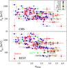 |
Fig. 1 Peak energy vs. PDS slope in the observer (top) and in the source rest-frame (bottom). Different colours correspond to different experiments. Filled squares (empty circles) correspond to power-law (broken power-law) models. Lower limits on α are given at 90% confidence. The only short available is also shown for comparison (diamond). |
All the PDS were calculated adopting the Leahy normalisation, in which the constant power due to uncorrelated statistical noise has a value of 2 for pure Poissonian noise (Leahy et al. 1983).
For each light curve we initially calculated the PDS by keeping the original minimum binning time for each experiment. After we made sure that no high-frequency (f ≳ 10 Hz) periodic feature stood out from the continuum, we decided to cut down the long computational time demanded by Monte Carlo simulations by binning up the light curves of Swift-BAT to 32 ms, equivalent to a Nyquist frequency fNy = 15.625 Hz. We did not adopt the potential alternative approach of binning up along frequency, after we noted that the corresponding distribution of power at high frequencies significantly deviated from the expected  , where M is the re-binning factor (van der Klis 1989). Unless stated otherwise, the PDS hereafter discussed were calculated in this way. Neither white-noise subtraction nor frequency re-binning was applied to the original PDS. Table 1 reports the time intervals used for the PDS calculation.
2.3. PDS modelling
We modelled the observed PDS following the procedure presented in the method paper (G16) based on a Bayesian MCMC technique, where two competing models are considered. The simpler one is a mere power-law (pl) plus the white-noise constant, 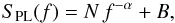 (1)where the following parameters were left free to vary: the normalisation constant N, the power-law index α (>0), and the white-noise level B. The PDS of several GRBs showed evidence of a break in the power law. For such cases, the procedure considers a model of a power law with a break, below which the PDS is asymptotically constant, which we here call bent power-law (bpl) model,
 ![Mathematical equation: \begin{equation} S_{\rm BPL}(f) = N\,\left[1 + \Big(\frac{f}{f_{\rm b}}\Big)^{\alpha}\right]^{-1} + B, \label{eq:mod_bpl} \end{equation}](/articles/aa/full_html/2016/05/aa27635-15/aa27635-15-eq49.png) (2)which reduces to the simple pl model of Eq. (1) in the limit f ≫ fb (α> 0). fb is the break frequency, below which the power density flattens. The preference for this model over the broken power-law model, such as that of Eq. (1) of Guidorzi et al. (2012) used for the average PDS, is provided in paper G16. A justification for the specific choice of Eq. (2) is that it provides a good description of the typical PDS of a fast rise exponential decay (FRED) pulse (e.g. Lazzati 2002).
(2)which reduces to the simple pl model of Eq. (1) in the limit f ≫ fb (α> 0). fb is the break frequency, below which the power density flattens. The preference for this model over the broken power-law model, such as that of Eq. (1) of Guidorzi et al. (2012) used for the average PDS, is provided in paper G16. A justification for the specific choice of Eq. (2) is that it provides a good description of the typical PDS of a fast rise exponential decay (FRED) pulse (e.g. Lazzati 2002).
A likelihood ratio test is used to establish whether a bpl provides a statistically significant improvement in the fit of a given PDS, with a 1% threshold on probability. We refer to G16 for a detailed description and justification of this method.
For GRBs with very good S/N and poor time resolution, such as HETE2-FREGATE whose Nyquist frequency is a mere 1.5 Hz, the white-noise level cannot be guessed from the GRB PDS. We therefore preliminarily estimated it from the PDS extracted over a different time interval adjacent to that of the GRB, including only background counts. Under the reasonable assumption that the temporal properties of background counts did not change, we constrained the white-noise level in the GRB PDS by means of a prior distribution for B.
3. Results
We rejected all the GRBs with σ(α) > 0.5, except for five GRBs (970508, 980425, 990712, 021211, and 030528) for which the 90%-confidence lower limit to α yielded a useful constraint. The selection on α was decided considering its observed range (1.3 <α< 3.9). This threshold allowed us to constrain the PDS slopes in a meaningful way. We ended up with 123 different GRBs with all measured and constrained Ep,i, Eiso, and α (and log fb for the GRBs with a break in the PDS), plus just one short from the Swift sample (Sect. 2.1.1). Twenty GRBs detected with both Fermi and Swift passed the PDS selection with both data sets. We used this sample to explore the effects of different energy bands and different time intervals. Best-fitting parameters are reported in Table 1. Some GRBs that were detected by both spacecraft are not classified as common, since only the data of one of the detectors matched our selection criteria. In these cases we reported the experiment whose data gave a useful PDS.
Sample of 123 GRBs.
Out of the observables and best-fitting parameters available we found a highly significant correlation between Ep,i and α, as displayed in the bottom panel of Fig. 1. Unsurprisingly, α also correlates with Eiso; however, the scatter is significantly larger, therefore hereafter we focus on Ep,i–α. For comparison, we also studied the observed peak energy, Ep = Ep,i/ (1 + z), vs. α, shown in the top panel of Fig. 1. For the 20 common GRBs we systematically chose the Fermi values for the broader energy passband. On average, the GRBs with higher Ep,i exhibit lower PDS indices. The p-values associated with Pearson, Spearman, and Kendall coefficients are 9 × 10⁻⁸, 1 × 10⁻⁸, and 2 × 10⁻⁸, respectively. These values do not account for the measurement uncertainties. We conservatively estimated their effect through MC simulations: we independently scattered each point assuming a log-normal distribution along Ep,i and using the marginal posterior distribution obtained for α for each GRB (see G16). We generated 1000 synthetic sets of 123 GRBs each and calculated the corresponding correlation coefficients. The 90% percentile values of the corresponding p-value distribution are reported in Table 2 both for the rest- and for the observer frame. The PDS index significantly correlates with both Ep,i and Ep. However, the significance of the correlation moves from 10-5 to 10-7–10-8 passing from observed to intrinsic plane, improving by almost three orders of magnitudes. We applied the same analysis to the subsample of pl GRBs alone to investigate whether the correlation still holds. We found that it does, with a p-value of the order of 10-6 in the source frame. Like for the overall sample, moving from the source to the observer frame the correlation becomes less significant by almost two orders of magnitude in this case (see Table 2).
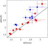 |
Fig. 2 PDS slope as measured with Swift-BAT and and with Fermi-GBM data for the common GRBs. Equality is shown for comparison (solid line). The GRBs whose best-fit models are equal (different) for both data sets are shown with squares (circles). |
Ep,i-(Ep-) α correlation significance.
Gamma-ray burst 060614 is worth mentioning. This is a clear outlier in a region of its own. This GRB is known to be peculiar for other observationally independent reasons: although it is classified as a long GRB, its nature yet remains ambiguous, since it shares some properties with short bursts, such as the absence of any associated supernova despite the small distance, the temporal lag of the initial spike (Gehrels et al. 2006; Della Valle et al. 2006; Fynbo et al. 2006), and the possible evidence for a macronova in the afterglow (Yang et al. 2015; Kisaka et al. 2016; Jin et al. 2015). Its prompt light curve consists of an initial hard spike followed by a soft variable tail, and it was shown to be consistent with the Ep,i-Eiso relation satisfied by most long GRBs only when the whole event is considered (Amati et al. 2007). By contrast, when only the negligible-lag spike is considered, its spectral and temporal properties are more reminiscent of short GRBs (Gehrels et al. 2006; Amati et al. 2007). If 060614 is excluded, the significance of the α-Ep,i correlation improves by a factor of a few (Table 2).
We also studied the covariance of the PDS slope with the spectral indices associated with the peak energy, derived from either a Band function or a cutoff power-law, and found no departure from statistical independence.
3.1. Dependence of PDS on energy band and on time interval
Figure 2 compares α as measured with Fermi and with Swift for the common sample of 20 GRBs.
The two main differences between Fermi-GBM and Swift-BAT are the broader and harder energy band for the former, along with a shorter time interval for the PDS calculation (Sects. 2.1 and 2.2). The role of the energy passband on determining the slope of GRB PDS is already known on the average PDS, with harder channels having lower α’s because of the more pronounced narrowness of their time profiles (Dichiara et al. 2013a). We therefore studied whether there is any link between the diversity of the two measures and the GRB hardness, as measured with Ep,i. We found no clear evidence for it. Rather than the GRB hardness itself, it is the combination of a longer time interval and a softer energy band of Swift-BAT that in most cases turns into the identification of a low-frequency break in the PDS. To clearly show this dependence, Fig. 2 displays the pairs of estimates with two different symbols, depending on whether the two best-fit models coincide. In all cases with different models, Swift data are best fit with a bpl while Fermi with a pl. These events, shown with circles in Fig. 2, deviate on average from equality more than the other GRBs, with higher values for Swift, as expected from the properties of average PDS (Dichiara et al. 2013a).
Yet, while the previously known average behaviour of PDS with energy is confirmed in the bulk properties of our common sample, we cannot infer a universal behaviour for all individual cases: for most common GRBs in Fig. 2Fermi and Swift PDS slopes are equal within uncertainties. This validates our choice of merging results obtained with different experiments into a unique set (Fig. 1). In conclusion, merging results obtained in different energy bands does not wash out the Ep,i − α correlation, but probably contributes to the observed scatter.
3.2. Selection effects
Since the correlation is highly scattered, we investigated the impact of selection effects that are due to S/N on the observed distribution of data on the Ep,i − α plane. Ideally, the S/N should be independent of both Ep,i and α. We therefore split the full sample into three different classes of S/N of 39 GRBs each with low (S/N< 52; hereafter SSN1), medium (52 <S/N< 121; SSN2), and high (S/N> 121; SSN3) values, and compared the distributions for the two variables in each subsample. We left out the five cases with lower limits derived for α plus one GRB from SSN3 to ensure that all samples had the same statistical accuracy from the same number of GRBs. We used the non-parametric Epps–Singleton (ES) test (Epps & Singleton 1986) to compute the probability that the Ep,i and α distributions of each sub-sample were drawn from a common one. We opted for ES instead of the more popular KS, because the latter is less sensitive than the former, especially for small samples. For Ep,i we found probabilities of 2%, 30%, and 43% for the comparisons SSN1-SSN2, SSN1-SSN3, and SSN2-SSN3 sub-sets, respectively. Thus we can state that the three Ep,i distributions are consistent with being drawn from a common population. Similar conclusions are drawn about α, with 82%, 38%, and 12% analogues probabilities, respectively. Finally, we computed the Ep,i − α correlation for the three samples (see Table 2) and found that the higher the S/N, the more significant the correlation. In other words, the better the signal, the less scattered the correlation, which means that the observed scatter is not entirely intrinsic to the sources, but is also due to the uncertainties affecting the individual measurements. This is clearly illustrated in Fig. 3 where we show the Ep,i − α distribution for the three S/N sub-samples along with their corresponding marginal distributions. We therefore conclude that the correlation is not spurious and cannot artificially be caused by S/N effects.
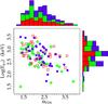 |
Fig. 3 Ep,i − α for three different classes of the light curve S/N. Blue circles, green diamonds, and red squares have high, middle, and low S/N, respectively. The corresponding histograms are shown along both axes. Error bars are not shown for the sake of clarity. |
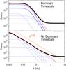 |
Fig. 4 Top panel: sketch of a bpl PDS (thick solid line) as the result of the superposition of PDS of different pulses (thin dashed lines). The overall variance is dominated by pulses with similar timescales (thick dashed lines), whose frequency break there corresponds to the dominant time. The white-noise level is also shown (dotted line). Bottom panel: the pl PDS is the result of the superposition of different pulses with different timescales, so that no break stands out in the total PDS, which looks like a power-law with a shallow index (α = 1.5 in this example, thick dashed line). |
4. Discussion
The choice of focusing on GRBs with well-measured Ep,i is driven by the key role of this observable in understanding the mechanism of the prompt emission. This is supported by a number of correlations in which Ep,i is involved: its correlation with Eiso (Amati et al. 2002), its time-resolved analogue (Golenetskii et al. 1983; Yonetoku et al. 2004; Ghirlanda et al. 2011; Lu et al. 2012; Frontera et al. 2012), with the collimation-corrected energy Eγ (Ghirlanda et al. 2004) for long GRBs, and both Eiso and the energy released in the X-ray band, EX,iso, in the three-parameter correlation, which holds for both long and short GRBs (Bernardini et al. 2012; Margutti et al. 2013). Thus, investigating the connection between Ep,i and temporal properties can provide clues on the physics of the prompt emission.
In Fig. 4 we illustrate our interpretation of the difference between the two groups of PDS best fit with either bpl or pl and the meaning of dominant timescale, wherever there exists one. Generally, a light curve is the result of superposing a number of pulses with different timescales. Whenever the total variance is dominated by some specific timescale, this stands out and determines the break in the PDS, which is best fit with bpl (top panel of Fig. 4). By contrast, when several different timescales have similar weights in the total variance, the resulting PDS exhibits no clear break, and appears to be remarkably shallower (αpl ≲ 2) than that of individual pulses (αbpl> 2). Most of the break frequency values correspond to timescales that are several second long. This suggests that most GRBs with a break in the PDS lack power at sub-second scales, which is not the case for the light curves of the pl group. Therefore, we interpret the two groups based on the relative strength of the short-timescale (<1 s; fast) component with respect to the long-timescale (>1 s; slow): GRBs of the bpl group exhibit weak or absent sub-second variability, whereas this is stronger in the pl group. Past works have reported evidence for two distinct (fast and slow) components in GRB light curves, with the fast component being stronger in the harder energy bands (Shen & Song 2003; Vetere et al. 2006; Gao et al. 2012). The correlation we found between PDS slope and Ep,i shows that GRBs with pronounced sub-second variability in addition to the slow component have, on average, higher peak energies.
The implications of our result can be discussed in the framework of some of the main prompt emission models. Considering the IS model, at given shell widths d and separations D, the higher the typical Lorentz factor, the correspondingly larger the IS radius ris ~ Γ2D, while the observed timescales still reflect the intrinsic inner engine variability. The easiest interpretation of our result is to invoke the bulk Lorentz factor as the key observable that explains the correlation between PDS and Ep,i. On the temporal side, we need to determine how Γ may be related to the fast component in the observed light curves. In early attempts to explain the luminosity-variability correlation (Fenimore & Ramirez-Ruiz 2000; Reichart et al. 2001; Guidorzi et al. 2005; Rizzuto et al. 2007), it was shown that the e± pair photosphere created by the IS synchrotron photons contributes to suppress the short-timescale variability in GRBs with lower Lorentz factors (Kobayashi et al. 2002; Mészáros et al. 2002). The radius of this photosphere is  (Γmin and Γmax are the Lorentz factors of the slowest and of the fastest shell). As a result, for
  (Dmin and Dmax are the smallest and the largest separation between shells) the first collisions for most shells take place below the pair photosphere. This turns into a wind of shells with ordered values of Γ that come out of the photosphere and can no longer effectively collide and produce bright and short pulses. On the other side, for
  most collisions occur above the photosphere, thus preserving the possibility of bright and short pulses in the observed light curve. The natural radiation mechanism in the optically thin region is synchrotron; in this case, Ep,i is the synchrotron peak energy and scales as
  , where γe and B are the electron Lorentz factor and the magnetic field in the fluid comoving frame, and L the luminosity. Since ris ∝ Γ2, the IS synchrotron model predicts Ep,i ∝ Γ-2 (Zhang & Mészáros 2002a; Ramirez-Ruiz & Lloyd-Ronning 2002), which clashes with our result. However, if Γ correlates with the jet-viewing angle, so that L ∝ Γmax, it is Ep,i ∝ Γ−3/2 as long as the fractions of internal energy taken by the magnetic field, ϵB, and by the accelerated electrons, ϵe, and the relative Lorentz factor of the colliding shells are constant. By letting them vary, it is possible to produce Ep,i ∝ Γ1/2 (Ramirez-Ruiz & Lloyd-Ronning 2002). Therefore, while our result cannot rule out the IS synchrotron model, its interpretation dictates specific constraints either in terms of continual acceleration of electrons in the shocked region, or on the dependence of ϵB and ϵe on Γ.
In the photospheric models the dissipation takes place below the photospheric radius at optical depths of a few to a few tens. Without going into the details of the various dissipation processes, we can identify two different origins for the prompt emission variability: (i) imprinted by the inner engine and (ii) resulting from the interaction of the jet with the stellar envelope and the cocoon (MacFadyen & Woosley 1999; Zhang et al. 2003; Lazzati & Begelman 2005; Morsony et al. 2010). The basic idea to explain our result still relies on the possibility that the inner engine can produce variable winds on sub-second timescales. If the spread in the observed Ep,i distribution is mainly driven by a geometric effect caused by different viewing angles θv and, therefore, correspondingly different photospheric radii, then lower peak energies, on average, correspond to larger θv (Lazzati et al. 2011, 2013). Our result suggests that the more off axis the observer, the weaker the expected high-frequency (>1 Hz) temporal power in the light curves. From detailed simulations that follow the jet propagation from inside the star all the way out to the photospheric radius, while the peak luminosity decreases at increasing θv, the high-frequency continuum power is generally described by a ν-2 behaviour and seemingly insensitive to θv (López-Cámara et al. 2014).
When at large distances (e.g. ~1015 cm in the ICMART model) the magnetisation is still high (σ ≳ 1), magnetic reconnection is more efficient than shocks in dissipating energy and accelerating non-thermal particles, as shown by recent particle-in-cell simulations (Sironi et al. 2015).
In the context of magnetic reconnection models for the GRB prompt emission, the essential idea that explains the observed variability is the relativistic motion (γ′ ≲ 10) of emitting clumps (or eddies, or fundamental emitters) within the bulk comoving frame. Since magnetic reconnection can be the source of turbulence (e.g. Lazarian et al. 2015), the emitting eddies have turbulent motions within the comoving frame of the outflow, as prescribed in the relativistic turbulence model (Lazar et al. 2009; Narayan & Kumar 2009; Kumar & Narayan 2009), At variance with the previous models, fast variability originates in the emission region (Lyutikov & Blandford 2003; Lyutikov 2006). The relative strength of the fast over the slow component reflects the filling factor of the eddies in the jet. Within this picture, our result suggests that GRBs with a large (low) filling factor, correspond to the high (low) Ep,i values. A possible problem with relativistic turbulence is that a large part of energy has to be continuously maintained in turbulent motion (Inoue et al. 2011). Moreover, since in its the original formulation this model assumes the eddy motions to be isotropically distributed in the shell frame, another problem concerns the pulse shape, which is expected to be symmetric and thereby at odds with observations, in which the decay is on average ~2–3 times longer than the rise (Norris et al. 1996). This problem can be solved when reconnection takes place in ordered thin layers between anti-parallel regions in the outflow (Beniamini & Granot 2015, hereafter BG15). In this model, magnetic reconnection is anisotropic in the shell comoving frame and isotropic in the emitter rest frame: the plasma in the reconnection region is accelerated to γ′ along the reconnection layer in the shell comoving frame, so that the higher γ′> 1, the more anisotropic the emission in the shell frame. They consider a thin shell as a reconnection layer that emits between R0 and R0 + ΔR. The duration of the pulse is given by T = max(ΔTr,ΔTθ), where ΔTr = ΔR/ 2cΓ2 and ΔTθ = R0/ 2cΓ2γ′ are the radial and the angular spreading times, respectively. For 1 /γ′ ≲ ΔR/R0, higher values of γ′ yield narrower, more symmetric, and more luminous (for a given total radiated energy) pulses. Hence, the higher γ′, the stronger the weight of short-timescales on the PDS. On the spectral side, the radiation process is mainly synchrotron, and the expected synchrotron frequency, in the observer frame, is ν ∝ ΓB′γ′2(1 − η) /η (where B′ is the magnetic field in the comoving shell frame). BG15 estimated η ~ 0.5 to explain the narrowing of pulses with energy, Δt ∝ E-0.4 (Fenimore et al. 1995), which implies ν ∝ ΓB′γ′2. Assuming that Ep,i scales as the synchrotron frequency, it is Ep,i ∝ ΓB′γ′2. Our result can be interpreted as follows: soft GRBs with a steep PDS are dominated by the slow component as the result of a relatively low relativistic magnetisation of the outflow at the dissipation site. Consequently, emitters are accelerated to only mildly relativistic energies in the shell comoving frame. By contrast, GRBs with shallower PDS mostly fit with pl model are the result of more energetic magnetic reconnection events to γ′ ~ 10. The large scatter of the Ep,i–α correlation can be attributed to the distribution of bulk Lorentz factor Γ, which varies from one GRB to another independently of γ′. That the correlation is mainly driven by γ′ rather than Γ can be explained by the quadratic dependence on γ′ (provided that B′ is independent). Moreover, a relatively narrow distribution in Γ further helps to enhance γ′ over Γ. This possibility seems plausible from the ≲0.2 dex scatter of the Γ distribution obtained from the afterglow peak interpreted as the fireball deceleration (Ghirlanda et al. 2012).
A similar conclusion can be derived considering another model that invokes a magnetically dominated dissipation. In the ICMART model (Zhang & Yan 2011) magnetised shells (σ> 1) collide at typical distances of classical IS (R ≳ 1015 cm), thus triggering cascades of turbulent reconnection. Here each broad pulse corresponds to a single cascade of mini-emitters triggered by the collision of two magnetised shells. The overall light curve of a multi-pulse GRB is explained by the occurrence of multiple independent shocks after the fashion of classical IS. As such, the time history on timescales of several seconds is ruled by the emission history of the inner engine. Each reconnection event behaves like a mini-emitter with a given  with respect to the outflow frame (Zhang & Zhang 2014). Interestingly, the calculated PDS of the individual light curves are fit with power laws, with occasional breaks at high frequencies. The simulated PDS slopes span from α ~ 1.1 to α ~ 2.1. Spikier curves have shallower PDS, as expected since high frequencies carry relatively more power than smoother light curves. Furthermore, the PDS slope is related in a simple way to the Lorentz factor contrast γ′/ Γ for a fixed Γ: for low contrasts (~0.01) the PDS slope is around 2, while for γ′/ Γ ~ 0.1 the PDS slope is around 1.1–1.2. On average, a more magnetised outflow (higher σ means higher γ′) seems to show a stronger fast or spiky component. On the other hand, Ep,i depends on γ′ as well (assuming the same spectrum in the emitter comoving frame), and is therefore correlated with the PDS slope.
5. Conclusions
We studied for the first time the individual PDS of a sample of 123 long GRBs with known distance and well-measured time-average spectrum. Using Bayesian MCMC techniques, we modelled the individual PDS with either a pl or a bpl model, depending on whether a break is required by a likelihood ratio test. We found a highly significant correlation between time-average rest-frame peak energy Ep,i and the PDS slope α, so that shallower PDS are associated with high Ep,i values. Moreover, GRBs with a break in the PDS, determined by the dominant timescale in the light curve, tend to be relatively soft (i.e. low values of Ep,i) and have steep PDS (above the frequency break). We interpret this to mean that the variety of PDS is mainly driven by the relative strength of a fast component in the light curves: the more variable the light curve at sub-second timescales, the shallower the PDS and the less likely a break in the explored range 0.01–1 Hz.
The only outlier GRB 060614 is noteworthy. This is known to be a peculiar nearby GRB with no associated SN that eludes the long-vs.-short classification. Future data of bright short GRBs together with a more detailed investigation of 060614 will help to clarify the behaviour of short GRBs in the Ep,i–α plane and add a new piece to the 060614 jigsaw.
We considered the main models that have been proposed in the literature to explain how or where GRB prompt emission originates, with emphasis on the distance from the progenitor. Overall, the most natural way to explain the Ep,i–α correlation is invoking a common (kinematic) origin, such as Doppler boosting. For photospheric models in which the dissipation takes place relatively close to the photosphere (1012–1013 cm), the fast component (when observed) keeps the memory of the variability imprinted by the inner engine. One possible interpretation suggested by our results is related to the viewing angle, so that the more off axis the observer, the weaker the fast (<1 s) variability component in the light curves, and the lower Ep,i.
Moving outwards to distances in the range from 1014 up to 1016 cm, there are different mechanisms, one of which is given by IS. Within the framework of the IS model, sub-second variability still reflects the inner engine character through the distribution of bulk Lorentz factor Γ of the wind of shells. The presence of an e± photosphere acts like a low-pass filter for a wind of shells with relatively low values of Γ (≈a few tens), whereas for a wind of fast shells (e.g. Γ of several hundreds) this would not be the case. Unless a dependence on Γ of microphysical parameters of the shock physics is invoked or specific assumptions are made, such as continuous electron acceleration in the shock region, the IS-predicted scaling Ep,i ∝ Γ-2 seems hardly compatible with the observed Ep,i–α correlation.
Magnetic reconnection as the dissipation mechanism of the GRB prompt emission is another option. The distance from the progenitor is comparably large as for the IS model, but in this case, the fast component originates in situ and the source of energy is magnetic rather than kinetic. The key to obtain sub-second variability at such large distance is the relativistic (γ′≲ 10) motion of emitters within the comoving frame of relativistic (Γ) shells. The details depend on the specific model: magnetic reconnection episodes could be triggered by shocks between magnetised shells after the fashion of the baryonic shells of the IS model, as envisaged in the ICMART model (Zhang & Yan 2011), or according to an anisotropic emission within the comoving frame of the reconnection layer (Beniamini & Granot 2015). In either case, the relative strength of the fast component in the observed curves relates to the average Lorentz factor γ′ of the emitters within the comoving shell frame, and hence to the magnetisation σ itself of the shell, rather than its bulk Lorentz factor Γ.
In summary, the relative strength of the fast component, which positively correlates with Ep,i and determines a shallow PDS, can probe the magnetisation of the outflow. In principle, this connection can be further tested by investigating other independent observables that may be affected by high values of σ, such as a reverse shock in the early afterglow (Zhang & Kobayashi 2005; Japelj et al. 2014), or large-scale magnetic fields entrained in the ejecta as revealed by prompt and early polarisation measurements (Mundell et al. 2007, 2013; Steele et al. 2009; Götz et al. 2009, 2014; Yonetoku et al. 2012; Uehara et al. 2012; Kopač et al. 2015). Ultimately, evidence for a highly magnetised jet can provide further support to scenarios where the GRB progenitor is a newly born millisecond magnetar.
To ensure a finite maximum in the νFν spectrum.
Acknowledgments
We thank the anonymous referee for helpful comments that improved the paper. S.D., C.G., L.A., F.F. acknowledge support by PRIN MIUR project on “Gamma Ray Bursts: from progenitors to physics of the prompt emission process”, P. I. F. Frontera (Prot. 2009 ERC3HT).
References
- Amati, L., Frontera, F., Tavani, M., et al. 2002, A&A, 390, 81 [NASA ADS] [CrossRef] [EDP Sciences] [Google Scholar]
- Amati, L., Della Valle, M., Frontera, F., et al. 2007, A&A, 463, 913 [NASA ADS] [CrossRef] [EDP Sciences] [Google Scholar]
- Amati, L., Guidorzi, C., Frontera, F., et al. 2008, MNRAS, 391, 577 [NASA ADS] [CrossRef] [MathSciNet] [Google Scholar]
- Band, D., Matteson, J., Ford, L., et al. 1993, ApJ, 413, 281 [NASA ADS] [CrossRef] [Google Scholar]
- Beloborodov, A. M. 2010, MNRAS, 407, 1033 [NASA ADS] [CrossRef] [Google Scholar]
- Beloborodov, A. M., Stern, B. E., & Svensson, R. 2000, ApJ, 535, 158 [NASA ADS] [CrossRef] [Google Scholar]
- Beniamini, P., & Granot, J. 2015, MNRAS, submitted [arXiv:1509.02192] [Google Scholar]
- Beniamini, P., & Piran, T. 2014, MNRAS, 445, 3892 [NASA ADS] [CrossRef] [Google Scholar]
- Bernardini, M. G., Margutti, R., Zaninoni, E., & Chincarini, G. 2012, MNRAS, 425, 1199 [NASA ADS] [CrossRef] [Google Scholar]
- Bošnjak, Ž., Götz, D., Bouchet, L., Schanne, S., & Cordier, B. 2014, A&A, 561, A25 [NASA ADS] [CrossRef] [EDP Sciences] [Google Scholar]
- Burrows, D. N., Grupe, D., Capalbi, M., et al. 2006, ApJ, 653, 468 [NASA ADS] [CrossRef] [Google Scholar]
- Della Valle, M., Chincarini, G., Panagia, N., et al. 2006, Nature, 444, 1050 [NASA ADS] [CrossRef] [PubMed] [Google Scholar]
- Derishev, E. V., Kocharovsky, V. V., & Kocharovsky, V. V. 1999, ApJ, 521, 640 [NASA ADS] [CrossRef] [Google Scholar]
- Dichiara, S., Guidorzi, C., Amati, L., & Frontera, F. 2013a, MNRAS, 431, 3608 [NASA ADS] [CrossRef] [Google Scholar]
- Dichiara, S., Guidorzi, C., Frontera, F., & Amati, L. 2013b, ApJ, 777, 132 [NASA ADS] [CrossRef] [Google Scholar]
- Epps, T. W., & Singleton, K. J. 1986, J. Statist. Comput. Sim., 26, 177 [CrossRef] [Google Scholar]
- Fenimore, E. E., & Ramirez-Ruiz, E. 2000, ArXiv e-prints [arXiv:astro-ph/0004176] [Google Scholar]
- Fenimore, E. E., in ’t Zand, J. J. M., Norris, J. P., Bonnell, J. T., & Nemiroff, R. J. 1995, ApJ, 448, L101 [NASA ADS] [CrossRef] [Google Scholar]
- Frontera, F., Guidorzi, C., Montanari, E., et al. 2009, ApJS, 180, 192 [NASA ADS] [CrossRef] [Google Scholar]
- Frontera, F., Amati, L., Guidorzi, C., Landi, R., & in’t Zand, J. 2012, ApJ, 754, 138 [NASA ADS] [CrossRef] [Google Scholar]
- Fynbo, J. P. U., Watson, D., Thöne, C. C., et al. 2006, Nature, 444, 1047 [NASA ADS] [CrossRef] [PubMed] [Google Scholar]
- Gao, H., Zhang, B.-B., & Zhang, B. 2012, ApJ, 748, 134 [NASA ADS] [CrossRef] [Google Scholar]
- Gehrels, N., Norris, J. P., Barthelmy, S. D., et al. 2006, Nature, 444, 1044 [NASA ADS] [CrossRef] [PubMed] [Google Scholar]
- Ghirlanda, G., Ghisellini, G., & Lazzati, D. 2004, ApJ, 616, 331 [NASA ADS] [CrossRef] [Google Scholar]
- Ghirlanda, G., Ghisellini, G., & Nava, L. 2011, MNRAS, 418, L109 [Google Scholar]
- Ghirlanda, G., Nava, L., Ghisellini, G., et al. 2012, MNRAS, 420, 483 [NASA ADS] [CrossRef] [Google Scholar]
- Giannios, D. 2008, A&A, 480, 305 [NASA ADS] [CrossRef] [EDP Sciences] [Google Scholar]
- Giannios, D. 2012, MNRAS, 422, 3092 [NASA ADS] [CrossRef] [Google Scholar]
- Goldstein, A., Burgess, J. M., Preece, R. D., et al. 2012, ApJS, 199, 19 [NASA ADS] [CrossRef] [Google Scholar]
- Golenetskii, S. V., Mazets, E. P., Aptekar, R. L., & Ilinskii, V. N. 1983, Nature, 306, 451 [NASA ADS] [CrossRef] [Google Scholar]
- Götz, D., Laurent, P., Lebrun, F., Daigne, F., & Bošnjak, Ž. 2009, ApJ, 695, L208 [NASA ADS] [CrossRef] [Google Scholar]
- Götz, D., Laurent, P., Antier, S., et al. 2014, MNRAS, 444, 2776 [NASA ADS] [CrossRef] [Google Scholar]
- Granot, J., Piran, T., Bromberg, O., Racusin, J. L., & Daigne, F. 2015, Space Sci. Rev., 191, 471 [NASA ADS] [CrossRef] [Google Scholar]
- Gruber, D., Goldstein, A., Weller von Ahlefeld, V., et al. 2014, ApJS, 211, 12 [NASA ADS] [CrossRef] [Google Scholar]
- Guidorzi, C., Frontera, F., Montanari, E., et al. 2005, MNRAS, 363, 315 [NASA ADS] [CrossRef] [Google Scholar]
- Guidorzi, C., Lacapra, M., Frontera, F., et al. 2011, A&A, 526, A49 [NASA ADS] [CrossRef] [EDP Sciences] [Google Scholar]
- Guidorzi, C., Margutti, R., Amati, L., et al. 2012, MNRAS, 422, 1785 [NASA ADS] [CrossRef] [Google Scholar]
- Guidorzi, C., Dichiara, S., & Amati, L. 2016, A&A, 589, A98 (G16) [NASA ADS] [CrossRef] [EDP Sciences] [Google Scholar]
- Guiriec, S., Connaughton, V., Briggs, M. S., et al. 2011, ApJ, 727, L33 [NASA ADS] [CrossRef] [Google Scholar]
- Guiriec, S., Kouveliotou, C., Daigne, F., et al. 2015, ApJ, 807, 148 [NASA ADS] [CrossRef] [Google Scholar]
- Huppenkothen, D., Watts, A. L., Uttley, P., et al. 2013, ApJ, 768, 87 [NASA ADS] [CrossRef] [Google Scholar]
- Inoue, T., Asano, K., & Ioka, K. 2011, ApJ, 734, 77 [NASA ADS] [CrossRef] [Google Scholar]
- Japelj, J., Kopač, D., Kobayashi, S., et al. 2014, ApJ, 785, 84 [NASA ADS] [CrossRef] [Google Scholar]
- Jin, Z. P., Yan, T., Fan, Y. Z., & Wei, D. M. 2007, ApJ, 656, L57 [NASA ADS] [CrossRef] [Google Scholar]
- Jin, Z.-P., Li, X., Cano, Z., et al. 2015, ApJ, 811, L22 [NASA ADS] [CrossRef] [Google Scholar]
- Kagan, D., Sironi, L., Cerutti, B., & Giannios, D. 2015, Space Sci. Rev., 191, 545 [NASA ADS] [CrossRef] [Google Scholar]
- Kaneko, Y., Preece, R. D., Briggs, M. S., et al. 2006, ApJS, 166, 298 [NASA ADS] [CrossRef] [Google Scholar]
- Kisaka, S., Ioka, K., & Nakar, E. 2016, ApJ, 818, 104 [NASA ADS] [CrossRef] [Google Scholar]
- Kobayashi, S., Ryde, F., & MacFadyen, A. 2002, ApJ, 577, 302 [NASA ADS] [CrossRef] [Google Scholar]
- Kopač, D., Mundell, C. G., Japelj, J., et al. 2015, ApJ, 813, 1 [NASA ADS] [CrossRef] [Google Scholar]
- Kumar, P., & Narayan, R. 2009, MNRAS, 395, 472 [NASA ADS] [CrossRef] [Google Scholar]
- Kumar, P., & Zhang, B. 2015, Phys. Rep., 561, 1 [NASA ADS] [CrossRef] [Google Scholar]
- Lazar, A., Nakar, E., & Piran, T. 2009, ApJ, 695, L10 [NASA ADS] [CrossRef] [Google Scholar]
- Lazarian, A., Eyink, G., Vishniac, E., & Kowal, G. 2015, Phil. Trans. Roy. Soc. London Ser. A, 373, 40144 [NASA ADS] [CrossRef] [Google Scholar]
- Lazzati, D. 2002, MNRAS, 337, 1426 [NASA ADS] [CrossRef] [Google Scholar]
- Lazzati, D., & Begelman, M. C. 2005, ApJ, 629, 903 [NASA ADS] [CrossRef] [Google Scholar]
- Lazzati, D., Morsony, B. J., & Begelman, M. C. 2011, ApJ, 732, 34 [NASA ADS] [CrossRef] [Google Scholar]
- Lazzati, D., Morsony, B. J., Margutti, R., & Begelman, M. C. 2013, ApJ, 765, 103 [NASA ADS] [CrossRef] [Google Scholar]
- Leahy, D. A., Darbro, W., Elsner, R. F., et al. 1983, ApJ, 266, 160 [NASA ADS] [CrossRef] [Google Scholar]
- López-Cámara, D., Morsony, B. J., & Lazzati, D. 2014, MNRAS, 442, 2202 [NASA ADS] [CrossRef] [Google Scholar]
- Lu, R.-J., Wei, J.-J., Liang, E.-W., et al. 2012, ApJ, 756, 112 [NASA ADS] [CrossRef] [Google Scholar]
- Lyutikov, M. 2006, MNRAS, 369, L5 [NASA ADS] [CrossRef] [Google Scholar]
- Lyutikov, M., & Blandford, R. 2003, ArXiv e-prints [arXiv:astro-ph/0312347] [Google Scholar]
- MacFadyen, A. I., & Woosley, S. E. 1999, ApJ, 524, 262 [NASA ADS] [CrossRef] [Google Scholar]
- Margutti, R., Zaninoni, E., Bernardini, M. G., et al. 2013, MNRAS, 428, 729 [NASA ADS] [CrossRef] [Google Scholar]
- McKinney, J. C., & Uzdensky, D. A. 2012, MNRAS, 419, 573 [Google Scholar]
- Meegan, C., Lichti, G., Bhat, P. N., et al. 2009, ApJ, 702, 791 [NASA ADS] [CrossRef] [Google Scholar]
- Mészáros, P., & Gehrels, N. 2012, Res. Astron. Astrophys., 12, 1139 [NASA ADS] [CrossRef] [Google Scholar]
- Mészáros, P., & Rees, M. J. 2011, ApJ, 733, L40 [NASA ADS] [CrossRef] [Google Scholar]
- Mészáros, P., Ramirez-Ruiz, E., Rees, M. J., & Zhang, B. 2002, ApJ, 578, 812 [NASA ADS] [CrossRef] [Google Scholar]
- Morsony, B. J., Lazzati, D., & Begelman, M. C. 2010, ApJ, 723, 267 [NASA ADS] [CrossRef] [Google Scholar]
- Mundell, C. G., Steele, I. A., Smith, R. J., et al. 2007, Science, 315, 1822 [NASA ADS] [CrossRef] [PubMed] [Google Scholar]
- Mundell, C. G., Kopac, D., Arnold, D. M., et al. 2013, Nature, 504, 119 [NASA ADS] [CrossRef] [Google Scholar]
- Narayan, R., & Kumar, P. 2009, MNRAS, 394, L117 [NASA ADS] [CrossRef] [Google Scholar]
- Narayan, R., Paczynski, B., & Piran, T. 1992, ApJ, 395, L83 [NASA ADS] [CrossRef] [Google Scholar]
- Norris, J. P., & Bonnell, J. T. 2006, ApJ, 643, 266 [NASA ADS] [CrossRef] [Google Scholar]
- Norris, J. P., Nemiroff, R. J., Bonnell, J. T., et al. 1996, ApJ, 459, 393 [NASA ADS] [CrossRef] [Google Scholar]
- Pe’er, A. 2015, Adv. Astron., 2015, 22 [NASA ADS] [Google Scholar]
- Pe’er, A., Mészáros, P., & Rees, M. J. 2006, ApJ, 642, 995 [NASA ADS] [CrossRef] [Google Scholar]
- Preece, R. D., Briggs, M. S., Mallozzi, R. S., et al. 2000, ApJS, 126, 19 [NASA ADS] [CrossRef] [Google Scholar]
- Ramirez-Ruiz, E., & Lloyd-Ronning, N. M. 2002, New Astron., 7, 197 [NASA ADS] [CrossRef] [Google Scholar]
- Rees, M. J., & Meszaros, P. 1994, ApJ, 430, L93 [NASA ADS] [CrossRef] [Google Scholar]
- Rees, M. J., & Mészáros, P. 2005, ApJ, 628, 847 [NASA ADS] [CrossRef] [Google Scholar]
- Reichart, D. E., Lamb, D. Q., Fenimore, E. E., et al. 2001, ApJ, 552, 57 [NASA ADS] [CrossRef] [Google Scholar]
- Rizzuto, D., Guidorzi, C., Romano, P., et al. 2007, MNRAS, 379, 619 [NASA ADS] [CrossRef] [Google Scholar]
- Rossi, E. M., Beloborodov, A. M., & Rees, M. J. 2006, MNRAS, 369, 1797 [NASA ADS] [CrossRef] [Google Scholar]
- Ryde, F., Borgonovo, L., Larsson, S., et al. 2003, A&A, 411, L331 [NASA ADS] [CrossRef] [EDP Sciences] [Google Scholar]
- Sakamoto, T., Barthelmy, S. D., Baumgartner, W. H., et al. 2011, ApJS, 195, 2 [NASA ADS] [CrossRef] [Google Scholar]
- Shen, R.-F., & Song, L.-M. 2003, PASJ, 55, 345 [NASA ADS] [CrossRef] [Google Scholar]
- Sironi, L., Petropoulou, M., & Giannios, D. 2015, MNRAS, 450, 183 [NASA ADS] [CrossRef] [Google Scholar]
- Soderberg, A. M., Berger, E., Kasliwal, M., et al. 2006, ApJ, 650, 261 [NASA ADS] [CrossRef] [Google Scholar]
- Steele, I. A., Mundell, C. G., Smith, R. J., Kobayashi, S., & Guidorzi, C. 2009, Nature, 462, 767 [NASA ADS] [CrossRef] [PubMed] [Google Scholar]
- Thompson, C. 1994, MNRAS, 270, 480 [NASA ADS] [CrossRef] [Google Scholar]
- Thompson, C., Mészáros, P., & Rees, M. J. 2007, ApJ, 666, 1012 [NASA ADS] [CrossRef] [Google Scholar]
- Titarchuk, L., Shaposhnikov, N., & Arefiev, V. 2007, ApJ, 660, 556 [NASA ADS] [CrossRef] [Google Scholar]
- Titarchuk, L., Farinelli, R., Frontera, F., & Amati, L. 2012, ApJ, 752, 116 [NASA ADS] [CrossRef] [Google Scholar]
- Uehara, T., Toma, K., Kawabata, K. S., et al. 2012, ApJ, 752, L6 [NASA ADS] [CrossRef] [Google Scholar]
- Usov, V. V. 1992, Nature, 357, 472 [NASA ADS] [CrossRef] [Google Scholar]
- van der Klis, M. 1989, in Timing Neutron Stars, eds. H. Ögelman, & E. P. J. van den Heuvel, 27 [Google Scholar]
- van Putten, M. H. P. M., Guidorzi, C., & Frontera, F. 2014, ApJ, 786, 146 [NASA ADS] [CrossRef] [Google Scholar]
- Vaughan, S. 2010, MNRAS, 402, 307 [NASA ADS] [CrossRef] [Google Scholar]
- Vaughan, S. 2013, Roy. Soc. London Phil. Trans. Ser. A, 371, 20110549 [NASA ADS] [CrossRef] [Google Scholar]
- Vetere, L., Massaro, E., Costa, E., Soffitta, P., & Ventura, G. 2006, A&A, 447, 499 [NASA ADS] [CrossRef] [EDP Sciences] [Google Scholar]
- Yang, B., Jin, Z.-P., Li, X., et al. 2015, Nature Commun., 6, 7323 [Google Scholar]
- Yonetoku, D., Murakami, T., Nakamura, T., et al. 2004, ApJ, 609, 935 [NASA ADS] [CrossRef] [Google Scholar]
- Yonetoku, D., Murakami, T., Gunji, S., et al. 2012, ApJ, 758, L1 [NASA ADS] [CrossRef] [Google Scholar]
- Zhang, B. 2014, Int. J. Mod. Phys. D, 23, 30002 [Google Scholar]
- Zhang, B., & Kobayashi, S. 2005, ApJ, 628, 315 [NASA ADS] [CrossRef] [Google Scholar]
- Zhang, B., & Mészáros, P. 2002a, ApJ, 581, 1236 [NASA ADS] [CrossRef] [Google Scholar]
- Zhang, B., & Mészáros, P. 2002b, ApJ, 571, 876 [NASA ADS] [CrossRef] [Google Scholar]
- Zhang, B., & Yan, H. 2011, ApJ, 726, 90 [NASA ADS] [CrossRef] [Google Scholar]
- Zhang, B., & Zhang, B. 2014, ApJ, 782, 92 [CrossRef] [Google Scholar]
- Zhang, W., Woosley, S. E., & MacFadyen, A. I. 2003, ApJ, 586, 356 [NASA ADS] [CrossRef] [Google Scholar]
All Tables
All Figures
|
Fig. 1 Peak energy vs. PDS slope in the observer (top) and in the source rest-frame (bottom). Different colours correspond to different experiments. Filled squares (empty circles) correspond to power-law (broken power-law) models. Lower limits on α are given at 90% confidence. The only short available is also shown for comparison (diamond). |
| In the text | |
|
Fig. 2 PDS slope as measured with Swift-BAT and and with Fermi-GBM data for the common GRBs. Equality is shown for comparison (solid line). The GRBs whose best-fit models are equal (different) for both data sets are shown with squares (circles). |
| In the text | |
|
Fig. 3 Ep,i − α for three different classes of the light curve S/N. Blue circles, green diamonds, and red squares have high, middle, and low S/N, respectively. The corresponding histograms are shown along both axes. Error bars are not shown for the sake of clarity. |
| In the text | |
|
Fig. 4 Top panel: sketch of a bpl PDS (thick solid line) as the result of the superposition of PDS of different pulses (thin dashed lines). The overall variance is dominated by pulses with similar timescales (thick dashed lines), whose frequency break there corresponds to the dominant time. The white-noise level is also shown (dotted line). Bottom panel: the pl PDS is the result of the superposition of different pulses with different timescales, so that no break stands out in the total PDS, which looks like a power-law with a shallow index (α = 1.5 in this example, thick dashed line). |
| In the text | |
Current usage metrics show cumulative count of Article Views (full-text article views including HTML views, PDF and ePub downloads, according to the available data) and Abstracts Views on Vision4Press platform.
Data correspond to usage on the plateform after 2015. The current usage metrics is available 48-96 hours after online publication and is updated daily on week days.
Initial download of the metrics may take a while.