| Issue |
A&A
Volume 588, April 2016
|
|
|---|---|---|
| Article Number | A61 | |
| Number of page(s) | 14 | |
| Section | Cosmology (including clusters of galaxies) | |
| DOI | https://doi.org/10.1051/0004-6361/201527431 | |
| Published online | 18 March 2016 | |
Quasar host environments: The view from Planck
1
DSM/Irfu/SPP, CEA-Saclay,
91191
Gif-sur-Yvette Cedex,
France
e-mail: This email address is being protected from spambots. You need JavaScript enabled to view it.
; This email address is being protected from spambots. You need JavaScript enabled to view it.
2
APC, AstroParticule et Cosmologie, Université Paris Diderot,
CNRS/IN2P3, CEA/lrfu, Observatoire de Paris, Sorbonne Paris Cité, 10 rue Alice Domon et Léonie
Duquet, 75205
Paris Cedex 13,
France
e-mail:
This email address is being protected from spambots. You need JavaScript enabled to view it.
3
Jet Propulsion Laboratory, California Institute of
Technology, 4800 Oak Grove
Drive, Pasadena,
California,
USA
Received: 23 September 2015
Accepted: 20 January 2016
Abstract
We measure the far-infrared emission of the general quasar (QSO) population using Planck observations of the Baryon Oscillation Spectroscopic Survey QSO sample. By applying multi-component matched multi-filters to the seven highest Planck frequencies, we extract the amplitudes of dust, synchrotron, and thermal Sunyaev-Zeldovich (SZ) signals for nearly 300 000 QSOs over the redshift range 0.1 <z< 5. We bin these individual low signal-to-noise measurements to obtain the mean emission properties of the QSO population as a function of redshift. The emission is dominated by dust at all redshifts, with a peak at z ~ 2, the same location as the peak in the general cosmic star formation rate. Restricting analysis to radio-loud QSOs, we find synchrotron emission with a monochromatic luminosity at 100 GHz (rest-frame) rising from  to 0.2 L⊙ Hz-1 between z = 0 and 3. The radio-quiet subsample does not show any synchrotron emission, but we detect thermal SZ between z = 2.5 and 4; no significant SZ emission is seen at lower redshifts. Depending on the supposed mass for the halos hosting the QSOs, this may or may not leave room for heating of the halo gas by feedback from the QSO.
Key words: cosmology: observations / large-scale structure of Universe / quasars: general / galaxies: clusters: general / methods: data analysis / methods: statistical
© ESO, 2016
1. Introduction
Quasars (or quasi stellar objects, QSOs) occupy a special place in large-scale structure and galaxy evolution (Kormendy & Richstone 1995). They are among the most luminous extra-galactic sources, and, as such, have become the focus of many cosmological surveys such as the 2dF Quasar Redshift Survey (2QZ; Croom et al. 2001) or the successive iterations of the Sloan Digital Sky Survey (SDSS I-IV; York et al. 2000; Eisenstein et al. 2011), where they provide a unique insight into the formation of structure on large scales and at high redshift (White et al. 2012). Quasars are likely powered (Salpeter 1964; Lynden-Bell 1969) by accretion of nearby matter onto supermassive black holes (SMBH, Rees 1984), whose evolution appears closely linked to the general cosmic star formation rate (Madau & Dickinson 2014), in particular in galaxies that contain a massive bulge (and therefore a massive central black hole) and a gas reservoir (Nandra et al. 2007; Silverman et al. 2008). The link is a clue to galaxy formation, its significance emphasized by the observed relation between the SMBH mass and galaxy properties (Ferrarese & Merritt 2000; Gebhardt et al. 2000). In addition, galaxy formation models must evoke strong feedback from active galactic nucleus (AGN) to explain the observed properties of massive galaxies and to avoid the overcooling catastrophe (Croton et al. 2006; Bower et al. 2006; McNamara & Nulsen 2007; Somerville et al. 2008; Fabian 2012; Blanchard et al. 1992)
Quasar environments give us a look at these powerful engines, and millimeter/submillimeter observations can offer a particularly revealing view of their effects: at these frequencies it is possible to study the cooler dust emission associated with star formation in the host, look for synchrotron emission from energetic particles, and, perhaps most pertinently, to measure energy feedback through observation of the thermal Sunyaev-Zeldovich (tSZ, Sunyaev & Zeldovich 1970, 1972) effect, a direct probe of the thermal energy contained in surrounding gas. Samples observed in this waveband with large ground-based facilities typically consist of, at most, several tens of objects (Omont et al. 2001, 2003, 2013; Isaak et al. 2002; Priddey et al. 2003; Beelen et al. 2006; Wang et al. 2007). Operating at these same frequencies, cosmic microwave background (CMB) surveys cover large sky areas and present the opportunity of studying much larger samples, albeit with much less detail of individual objects. We can, however, determine the average properties of large representative populations, a valuable compliment to the more detailed examinations.
The Wilkinson Microwave Anisotropy Probe (WMAP, Bennett et al. 2003) and Planck missions (Tauber et al. 2010; Planck Collaboration I 2011) are ideal for this purpose because of their all-sky coverage, including the entire SDSS (York et al. 2000) area. Cross-correlating WMAP data with photometric QSOs from SDSS data release 3 (DR3), Chatterjee et al. (2010) finds evidence at 2.5σ for the tSZ effect from QSO environments. Ruan et al. (2015) improved the significance using a publicly available tSZ map (Hill & Spergel 2014) constructed from the Planck mission dataset and 26 686 spectroscopic QSOs from SDSS DR7. They concluded that the total thermal energy feedback into surrounding gas was significantly larger than expected according to galaxy formation models, which is consistent with the findings of Chatterjee et al. (2010). Planck’s wide frequency coverage, from 30 GHz to 857 GHz, is a distinct advantage for disentangling the different sources of emission from the QSO environment, and was implicitly exploited by Ruan et al. (2015) when using the tSZ map published by Hill & Spergel (2014).
Although not all-sky, the Atacama Cosmology Telescope (ACT) surveyed several hundred square degrees near the celestial equator, overlapping AGN and QSO samples in the North. Gralla et al. (2014) stacked millimeter maps from ACT over this area of radio-loud AGN seen in the FIRST and NVSS radio surveys to find a tSZ signal at 5σ significance. More recently, and in parallel to our present study, Crichton et al. (2015) combined ACT and Herschel data of radio-quiet quasars in the SDSS DR7 and DR10 samples, detecting the tSZ signal at 3−4σ significance.
In this paper, we use the full-mission Planck frequency maps to examine the emission properties of the SDSS-III Baryon Acoustic Oscillation (BOSS, Dawson et al. 2013) DR12 QSO sample. We extract not only the tSZ signal from the population, but also dust and synchrotron emission by stacking measurements made with a set of matched filters directly applied to the seven highest frequency Planck channels. The joint extraction enables us to study not only the gas thermal environment, but star formation conditions and the production of energetic particles. Moreover, it improves analysis robustness by giving information on correlations between the observed signals, compared to the use of a tSZ map. Ruan et al. (2015) were in fact faced with the difficulty of correcting the SZ map for contamination from dust emission.
We extend our multi-matched filter (MMF, Melin et al. 2006; see also Herranz et al. 2002) formalism to simultaneously extract two or three emission components, following development started in Planck Collaboration Int. XI (2013). Stacking the various signals to study their evolution with redshift, we reconstruct for the first time a picture of the evolution of the dust signal, the synchrotron emission, and the tSZ effect between z ~ 0 and z ~ 5 for the general QSO population.
In Sect. 2, we describe the BOSS and Planck datasets. We detail the analysis methods and tools in Sect. 3. In Sect. 4, we apply them on simulations. Results on Planck data are given in Sect. 5. We discuss our results in Sect. 6 and conclude in Sect. 7. Throughout, we use the spatially flat base ΛCDM cosmology from Planck Collaboration XIII (2015): H0 = 67.27 = h100 km s-1/Mpc, Ωm = 0.3156, Ωbh2 = 0.02225 and σ8 = 0.831.
2. Data
2.1. BOSS quasars
One of the major goal of the SDSS-III Baryon Oscillation Spectroscopic Survey (BOSS) is the production of a QSO catalogue to detect the BAO scale in the Lyman-α forests at redshift z ~ 2.5. A first detection was made on the DR9 QSO catalogue (Pâris et al. 2012) by Busca et al. (2013), confirmed latter by Delubac et al. (2015). In this study, we use the recently published DR12 QSO catalogue1 (Alam et al. 2015).
The sources are detected and selected with the CCD imaging Camera installed in the Sloan Foundation 2.5 m Telescope at Apache Point observatory, New Mexico. The spectra of each source is measured with the BOSS spectrograph which covers wavelength between 3600 Å and 10 000 Å. Spectra measurement leads to the computation of the spectroscopic redshift and the checking of the nature of the source.
The DR12 QSO catalogue contains 297 301 objects. We remove 5880 QSO falling outside the Planck 65% mask, in a region strongly contaminated by the Milky Way dust. Finally, we also reject 256 QSO because they are at low redshift z< 0.1 so may be partially resolved by Planck , because they belong to the high redshift (z> 5) population or because they have a bad estimate of the magnitude in g band (g< 0) . We thus use a catalogue of 291 165 QSO in the redshift range 0.1 <z< 5. The distribution of the QSO in term of redshift is not flat and reach two notable maxima at z = 0.8 and z = 2.3 (Fig. 1).
The target selection was developed to select quasars with an observable Ly-α forest (i.e. quasars with z> 2.2). However, degeneracies in the color-redshift relation of quasars led to the selection of low-z quasars in BOSS (Fig. 1). The quasars at z ~ 0.8 have MgII λ2800 line at the same wavelength as Ly-α at redshift z ~ 3.1, giving these objects similar broadband colors, while the large number of objects at z ~ 1.6 is due to the confusion between λ1549 C-IV line and Ly-α at z ≈ 2.3 (Ross et al. 2012). In contrast, the selection based on the intrinsic variability of quasars gives a more uniform distribution in redshift (Palanque-Delabrouille et al. 2011).
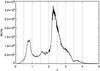 |
Fig. 1 Redshift distribution of the BOSS DR12 QSO sample. The distribution presents two peaks, at z ~ 0.8 and z ~ 2.3, due to the QSO target selection process (see text). The regular binning used throughout this paper (Δz = 0.5) is shown as the vertical dotted lines. |
2.2. Planck maps
The Planck satellite was launched in May 2009 (Tauber et al. 2010). After traveling to the Earth-Sun Lagrange point L2, it scanned the entire sky continuously from August 2009 to October 2013 in nine frequency bands ranging from 30 to 857 GHz. The primary goal of the mission was to study the primary CMB anisotropies, but its large frequency coverage also enables unique Galactic and extra-galactic astrophysical studies. In particular, the High Frequency Instrument (HFI, Lamarre et al. 2010; Planck HFI Core Team IV. 2011), covering bands from 100 to 857 GHz, is ideally suited for Sunyaev-Zeldovich science. Moreover, the three highest frequencies (353 to 857 GHz) of the instrument pick up Galactic and extra-galactic dust emission. The Low Frequency Instrument (LFI, Bersanelli et al. 2010; Mennella et al. 2011), with channels at 30, 44, 70 GHz, is sensitive to synchrotron, free-free, and spinning dust emission.
We use the seven highest frequency (70, 100, 143, 217, 353, 545, and 857 GHz) full-sky maps from the 2015 data release (Planck Collaboration I 2015; Planck Collaboration VIII 2015; Planck Collaboration VI 2015). These bands are the best suited to study the dust, gas, and synchrotron emission from high redshift QSO environments. The substantially larger beams of the remaining 30 and 40 GHz channels make them less well adapted for studying what are essentially point sources. We divide each Planck HEALPix2 all-sky map into 504 overlapping flat tangential patches of 10 × 10 degrees with a 1.72 arcmin pixel scale in order to apply our extraction algorithms described in Sect. 3.2.
3. Analysis
Determining the physical properties of the QSO environment from the Planck maps faces two major challenges. The first is the faint QSO flux in the Planck maps, far below the noise level; individual detection is not possible. We thus have to use a statistical approach similar to the one developed in Melin et al. (2011) and subsequently in Planck Collaboration X (2011), Planck Collaboration XII (2011), Planck Collaboration Int. XI (2013). Details of the approach are given in Sect. 3.4.1.
The second challenge arises from the superposition of different emission sources from the QSO in the Planck beams: emission from dust located inside the host galaxy or possibly at larger scale in the host halo of the QSO; synchrotron emission from the host galaxy or from relativistic outflows of the central AGN; and the tSZ effect due to the hot gas surrounding the QSO and within the host halo. Planck does not have the spatial resolution to separate these components, but its good spectral coverage enables us to disentangle these sources of emission.
We separate the signals using multi-component matched multi-filters (MMF), an extension of the approach used in Planck Collaboration Int. XI (2013). The detailed description is given in Sect. 3.2.2. We will see that the QSO signal in Planck is dominated by dust emission, but that we also detect both synchrotron and tSZ signals. In practice, we proceed as follows:
-
1.
assume that the QSO signal is a mixture of one, two or three components;
-
2.
apply the adapted multi-component MMF at each QSO position to obtain the amplitude of each component;
-
3.
bin average (as a function of redshift or magnitude) these amplitudes over the QSO sample;
-
4.
evaluate the ability of our model to describe the data using a χ2-test (see Sect. 3.4.2).
Our notation in the subsequent sections is as follows. We use the letter p as index to denote individual QSOs in the catalogue and the indices i and j to denote observation frequencies. The Greek indices λ and μ specify the nature of the emission components, e.g., λ and μ have as possible values dust, synch, and tSZ for dust, synchrotron, and tSZ signals, respectively.
3.1. Model of the QSO emission
We model the QSO emission as a sum of dust, synchrotron, and tSZ signals. The seven-frequency column vector map, m(x), at position x on the sky is written as 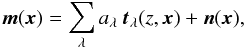 (1)where aλ is the amplitude of the λ component, tλ(z,x) is the associated, normalized emission vector, z the redshift of the QSO, and n(x) is the astrophysical and instrumental noise. We center the QSO in the map to simplify the expressions. The ith component of each emission vector is the signal profile, τλ (normalized to unity at the origin), convolved by the Planck beam, bi (normalized to unity at the origin), at frequency νi, and then scaled by the expected frequency dependance
  :
: . \end{eqnarray}](/articles/aa/full_html/2016/04/aa27431-15/aa27431-15-eq54.png) (2)We describe the dust emission frequency dependence by a modified blackbody, the synchrotron emission by a power law, and we use the non-relativistic calculation for the tSZ (e.g., Birkinshaw 1999; Carlstrom et al. 2002):
(2)We describe the dust emission frequency dependence by a modified blackbody, the synchrotron emission by a power law, and we use the non-relativistic calculation for the tSZ (e.g., Birkinshaw 1999; Carlstrom et al. 2002): ![Mathematical equation: \begin{eqnarray} &&\left(S_{\rm d}\right)_i(z) = \left ({\nui \over 857~{\rm GHz}} \right )^{\beta_{\rm d}} {B_{\nui}[T_{\rm d}/(1+z)] \over B_{857~{\rm GHz}} \, [T_{\rm d}/(1+z)]}, \\ &&\left(S_{\rm s}\right)_i= \left ( {100~{\rm GHz} \over \nu_i } \right )^{\alpha_{\rm s}},\\ &&\left(S_{\rm sz}\right)_i= B_{\nui}(T_{\rm cmb}){x_i e^{x_i} \over e^{x_i}-1} \left [ {x_i \over \tanh(x/2)} - 4 \right], \end{eqnarray}](/articles/aa/full_html/2016/04/aa27431-15/aa27431-15-eq55.png) where xi = hνi/kTcmb with Tcmb the temperature of the CMB today, Bν(T) represents the Planck spectrum, Td and βd are the dust temperature and emissivity index, and αs = 0.7 for the synchrotron index. It is the typical value for radio galaxies (Condon 1992; Peterson 1997). We note that the first two expressions are unitless, so that adust and asynch carry units of brightness; on the other hand, StSZ carries brightness units while atSZ is unitless and corresponds to the central Compton-y parameter.
where xi = hνi/kTcmb with Tcmb the temperature of the CMB today, Bν(T) represents the Planck spectrum, Td and βd are the dust temperature and emissivity index, and αs = 0.7 for the synchrotron index. It is the typical value for radio galaxies (Condon 1992; Peterson 1997). We note that the first two expressions are unitless, so that adust and asynch carry units of brightness; on the other hand, StSZ carries brightness units while atSZ is unitless and corresponds to the central Compton-y parameter.
We adopt the same spatial profile for all signal templates, τλ = τ(x/θf), where τ is taken from Arnaud et al. (2010) based on the observed cluster halos gas pressure profile. We fix θf = 0.27 arcmin, the value corresponding to a halo of mass M500 = 1013M⊙ at z = 2. This value is smaller than the smallest Planck beam (fwhm = 4.2 arcmin at 857 GHz): the bulk of the QSO remain unresolved by Planck. We study the sensitivity of our results to this fixed size in Sect. 5.5. The profiles are cut at θ> 5θ500.
In the following we therefore denote this universal QSO profile by τqso. We are then able to define the QSO brightness, f, as the sum over the different components as 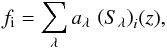 (6)and rewrite the map at frequency i as
 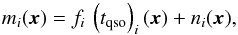 (7)where
 $}](/articles/aa/full_html/2016/04/aa27431-15/aa27431-15-eq78.png) .
.
3.2. Matched filters
3.2.1. Single frequency matched filter
We use single frequency matched filters to extract individual QSO signals (at S/N ≪ 1) at each Planck frequency. The individual signals are necessary to compute the χ2 statistic described in Sect. 3.4.2. We also average them to obtain the mean QSO spectrum in Sect. 5.
The single frequency matched filter is a linear filter designed to return an unbiased signal estimate with minimal error (Haehnelt & Tegmark 1996; Sanz et al. 2001). No assumption is made concerning the frequency dependance of the signal. The estimated value,  , of the true signal, fi, is
  (8)where Ψi(x) is the matched filter for frequency νi. The filter Ψi is expressed in Fourier space as
 ![Mathematical equation: \begin{equation} \Psi_{\rm i}(\vec{k}) = \sigma^2[ \hat{f}_{\rm i}] \frac{\left(t_{\rm qso}^{*}\right)_i(\vec{k}) }{P_{ii}(\vec{k})}, \end{equation}](/articles/aa/full_html/2016/04/aa27431-15/aa27431-15-eq85.png) (9)with the error on the estimated signal
(9)with the error on the estimated signal ![Mathematical equation: \begin{eqnarray} \label{eq:sigt_flux} \sigma[\hat{f}_{\rm i} ] && \equiv \sqrt{ \langle{ \hat{f}_{\rm i}^2 \rangle} - \langle{ \hat{f}_{\rm i} \rangle}^2} \nonumber\\ & = & \left[\int {\rm d}^2k\; \frac{ \left| \left(t_{\rm qso}\right)_i(\vec{k}) \right|^2}{P_{ii}(\vec{k})}\right]^{-1/2}, \end{eqnarray}](/articles/aa/full_html/2016/04/aa27431-15/aa27431-15-eq86.png) (10)where Pii(k) is the noise power spectrum of the ith Planck map, mi(k). Because the signal-to-noise of an individual QSO signal is smaller than unity, we estimate Pii(k) directly as the power spectrum of the map.
(10)where Pii(k) is the noise power spectrum of the ith Planck map, mi(k). Because the signal-to-noise of an individual QSO signal is smaller than unity, we estimate Pii(k) directly as the power spectrum of the map.
3.2.2. Matched multi-filters
The MMF were first introduced by Herranz et al. (2002) for SZ detection. They were further developed by Melin et al. (2006) and extensively used to construct the successive Planck SZ cluster catalogs (Planck Collaboration VIII 2011; Planck Collaboration XXIX 2014; Planck Collaboration XXVII 2015). The MMF target the extraction of a single component across a set of maps, assuming a known frequency dependance and a spatial distribution. The filtered map returns a unbiased estimate, âλ, of aλ with minimal variance:  (11)Similarly to the single frequency case, the MMF for the λ emission, Ψλ(x), is expressed in Fourier space as
 ![Mathematical equation: \begin{equation} \vec{{\Psi}}_{\lambda}(\vec{k}) = \sigma^2[\hat{a}_{\lambda}] \, \mathbf{P}^{-1}(\vec{k})\cdot \vec{t_{\lambda}^{*}}(z,\vec{k}). \end{equation}](/articles/aa/full_html/2016/04/aa27431-15/aa27431-15-eq92.png) (12)The error on the amplitude is now given as
(12)The error on the amplitude is now given as ![Mathematical equation: \begin{eqnarray} \label{eq:sigt} \sigma[\hat{a}_{\lambda}] && \equiv \sqrt{ \langle{ \hat{a}_{\lambda}^2 \rangle} - \langle{ \hat{a}_{\lambda} \rangle}^2} \nonumber\\ &=& \left[\int {\rm d}^2k\; \vec{t_{\lambda}^{*}}^{t}(z,\vec{k})\cdot \mathbf{P}^{-1}(\vec{k}) \cdot \vec{t_{\lambda}}(z,\vec{k})\right]^{-1/2}, \end{eqnarray}](/articles/aa/full_html/2016/04/aa27431-15/aa27431-15-eq93.png) (13)with P(k) being the inter-band cross-power spectrum matrix with contributions from (non-λ) sky signal and instrumental noise. It is the effective noise matrix for the MMF and, as for the single frequency power spectrum, can be estimated directly on the data, since the λ signal (dust, synchrotron or tSZ) is small compared to other astrophysical signals over the sky patch.
(13)with P(k) being the inter-band cross-power spectrum matrix with contributions from (non-λ) sky signal and instrumental noise. It is the effective noise matrix for the MMF and, as for the single frequency power spectrum, can be estimated directly on the data, since the λ signal (dust, synchrotron or tSZ) is small compared to other astrophysical signals over the sky patch.
Introduced in Planck Collaboration Int. XI (2013) for a mixture of dust and tSZ signals, multi-component filtering deals with different MMF to separate dust and tSZ signals. Multi-component filtering has also been successfully used to jointly extract the tSZ and kinetic SZ (kSZ) effects in Planck Collaboration Int. XIII. (2014). For these filters, the recovered amplitude of each component is unbiased with minimal variance if the assumption on the number and type of the components is correct.
We consider three multi-component filtering schemes: 1) dust + tSZ; 2) dust + synchrotron; and 3) dust + tSZ + synchrotron filters. The amplitudes aλ are estimated using a linear combination of the partial MMFs, ![Mathematical equation: \begin{equation} \hat{a}_{\lambda} = \sum_{\mu}{ \left[\vec{D}^{-1} \right]_{\lambda, \mu}\, \int {\rm d}^2x \; \vec{{\Phi}}_{\mu}^t(\vec{x}) \cdot \vec{m}(\vec{x})}, \end{equation}](/articles/aa/full_html/2016/04/aa27431-15/aa27431-15-eq96.png) (14)with the partial MMF defined in Fourier space by
(14)with the partial MMF defined in Fourier space by  (15)and the matrix D computed as
 ![Mathematical equation: \begin{equation} D_{\lambda, \mu} = \left[\int {\rm d}^2k\; \vec{t_{\lambda}^{*}}^t(z,\vec{k})\cdot \mathbf{P}^{-1}(\vec{k}) \cdot \vec{t_{\mu}}(z,\vec{k})\right]. \end{equation}](/articles/aa/full_html/2016/04/aa27431-15/aa27431-15-eq99.png) (16)The estimated amplitudes are combined together in a N-component vector (N being the number of signal components considered),
(16)The estimated amplitudes are combined together in a N-component vector (N being the number of signal components considered),  . They are correlated with covariance matrix
 ![Mathematical equation: \begin{eqnarray} \label{eq:sigt_cross} C[\hat{\vec{a}}]_{\lambda, \mu} & & \equiv \langle{ \hat{a}_{\lambda} \hat{a}_{\mu} \rangle} - \langle{ \hat{a}_{\lambda} \rangle}\langle{ \hat{a}_{\mu}\rangle} \nonumber\\ & = &\left[\vec{D}^{-1} \right]_{\lambda, \mu}. \end{eqnarray}](/articles/aa/full_html/2016/04/aa27431-15/aa27431-15-eq102.png) (17)In summary, we use the single frequency matched filter plus the following five filters in our study:
(17)In summary, we use the single frequency matched filter plus the following five filters in our study:
-
single component MMF for dust;
-
single component MMF for tSZ;
-
two-component MMF for dust + tSZ;
-
two-component MMF for dust + synchrotron;
-
three-component MMF for dust + tSZ + synchrotron.
3.3. From observed signals to physical QSO properties
The amplitudes âλ (determined with profiles cut at θ< 5θ500) are converted into spherically integrated quantities within R500 by  (18)where the factor Cλ(5R500 → R500) is the conversion from the volume within 5R500 to R500, given the adopted profile. Similarly, we obtain the source flux density vector,
  , as
, as  (19)We express the quantities
  ,
,  , and
, and  in mJy and
  in arcmin2.
Following Beelen et al. (2006) we estimate the total dust mass of the QSO from  as
as ![Mathematical equation: \begin{equation} \estMd=\widehat{A}_{\rm dust}{D_{\rm L}(z)^2 \over (1+z)}\kappa^{-1}\left[857\,{\rm GHz}(1+z)\right] B_{857~{\rm GHz}(1+z)}^{-1}(T_{d}), \label{eq:mdust} \end{equation}](/articles/aa/full_html/2016/04/aa27431-15/aa27431-15-eq116.png) (20)with
(20)with  , κ0 = 0.4 g-1 cm2 and DL(z) the luminosity distance. From the synchrotron flux density at 100 GHz, we compute the monochromatic synchrotron luminosity according to
  (21)which is referenced to the rest-frame frequency of 100 GHz assuming our power law with αs.
We define the intrinsic Compton parameter,  , as the quantity
  from Planck Collaboration Int. XI (2013),
  (22)DA(z) being the angular distance to the QSO in Mpc. Applying Eq. (22) of Arnaud et al. (2010), we estimate the total mass of the halo as
 ![Mathematical equation: \begin{equation} \estMfive = (1-b) \widehat{M}_{500,{\rm true}} = 3 \times 10^{14} \left ( {h \over 0.7} \right ) ^{-1} {\left[{\widehat{\rm A}_{\rm tSZ} E(z)^{-2/3} \over A_{\rm x}(z)}\right]}^{1/\alpha} M_{\odot} , \label{eq:mhalo} \end{equation}](/articles/aa/full_html/2016/04/aa27431-15/aa27431-15-eq126.png) (23)with α = 1.78 and
(23)with α = 1.78 and  . The so-called mass bias parameter, b, accounts for any bias between the estimated mass and the true halo mass, M500,true, for example from violation of hydrostatic equilibrium and/or X-ray instrument calibration. Planck SZ cluster counts require high values of the mass bias, (1 − b) ~ 0.6−0.7, for consistency with the base ΛCDM model favored by Planck’s measurements of the primary CMB anisotropies (see Planck Collaboration XX 2014; Planck Collaboration XXIV 2015, and references therein).
The  relation can be derived from the last two equations:
 ![Mathematical equation: \begin{equation} \frac{\estMfive}{10^{13} \, M_{\odot}}= \left( \frac{h}{0.7}\right)^{1/\alpha-1} \left[\frac{\widehat{Y}_{500} }{2.00 \times 10^{-6} \, {\rm arcmin}^2}\right]^{1/\alpha}\cdot \label{eq:ymhalo} \end{equation}](/articles/aa/full_html/2016/04/aa27431-15/aa27431-15-eq133.png) (24)
(24)
3.4. Statistics
3.4.1. Average values for the full QSO sample
As described before, the individual QSO signals are expected to be faint, so we need to average them over the population. Here, we detail the computation of this average. We adopt the generic notation ŵλ for  ,
,  ,
,  , or
, or  , arranging them into a vector
  , and assume that they are Gaussian distributed.
If these different components of are not correlated, we employ the usual inverse-variance weighted average: ![Mathematical equation: \begin{eqnarray} &&\langle \hat{w}_{\rm \lambda} \rangle= \left[\sum_{p}{\frac{1}{\sigma^2[\left(\hat{w}_{\lambda}\right)_{p}]}}\right]^{-1} \left[\sum_{p}{\frac{\left(\hat{w}_{\lambda}\right)_{p}}{\sigma^2[\left(\hat{w}_{\lambda}\right)_{p}]}}\right], \\ &&\sigma[\langle{\hat{w}_{\lambda}\rangle}]= \sqrt{\left[\sum_{p}{\frac{1}{\sigma^2[\left(\hat{w}_{\lambda}\right)_{p}]}}\right]^{-1}} , \end{eqnarray}](/articles/aa/full_html/2016/04/aa27431-15/aa27431-15-eq140.png) with p the index over the QSO catalogue.
with p the index over the QSO catalogue.
In the correlated case, the average values are obtained according to ![Mathematical equation: \begin{eqnarray} \label{eq:average_correlation} &&\langle{\vec{\hat{w}} \rangle}= \left[\sum_{p}{\vec{C}^{-1}[\left(\hat{\vec{w}}\right)_{p}]}\right]^{-1} \cdot \left[\sum_{p}{\vec{C}^{-1}[\left(\hat{\vec{w}}\right)_{p}] \cdot \left(\hat{\vec{w}}\right)_{p}} \right], \\ \label{eq:sigma_average_correlation} &&\vec{C}[\langle{\vec{\hat{w}} \rangle}]= \left[\sum_{p}{\vec{C}^{-1}[\left(\hat{\vec{w}}\right)_{p}]}\right]^{-1}. \end{eqnarray}](/articles/aa/full_html/2016/04/aa27431-15/aa27431-15-eq141.png)
3.4.2. χ2-test for the hypothesis
If the assumptions on the nature and number of components are correct, the measured flux densities,  , and the reconstructed model flux densities,
  , must be consistent within the uncertainties. We introduce the residual flux density for a given QSO as
  (29)Correlation between the measured flux densities, , and the model amplitudes,
  , leads to the following expression for the variance of the residuals:
 ![Mathematical equation: \begin{eqnarray} C[\vec{R}]_{i j} && \equiv \langle{{R_{i}} {R_{j}} \rangle} -\langle{{R_{i}} \rangle}\langle{{R_{j}} \rangle}\nonumber \\ & =& C[\widehat{\vec{F}}]_{i j} - \sum_{\lambda, \mu}{ \left({S}_{\lambda}\right)_{i}(z) C[\vec{\widehat{A}}]_{\lambda, \mu} \left({S}_{\mu}\right)_{j}(z)}, \end{eqnarray}](/articles/aa/full_html/2016/04/aa27431-15/aa27431-15-eq147.png) (30)where
(30)where ![Mathematical equation: \begin{eqnarray} C[\widehat{\vec{F}}]_{i j} & & \equiv \langle{{\widehat{F}_{i}} {\widehat{F}_{j}} \rangle}- \langle{{\widehat{F}_{i}} \rangle}\langle{{\widehat{F}_{j}} \rangle} \nonumber\\ & = & N_{R_{500}} \left[\int {\rm d}^2k\; \frac{ \left({t_{\rm qso}^{*}}\right)_{i}(\vec{k}) \, \left({t_{\rm qso}}\right)_{j}(\vec{k}) \, {P_{i j}(\vec{k})} }{{P_{ii}(\vec{k})} \, {P_{jj}(\vec{k})}}\right]^{-1}, \end{eqnarray}](/articles/aa/full_html/2016/04/aa27431-15/aa27431-15-eq148.png) (31)with NR500 = ∫r<R500dr4πr2τqso(r). The residuals Ri are expected to be Gaussian distributed with zero mean. We employ Eqs. (27) and (28) with R, instead of ŵ, to compute the average value, and define the χ2 for the average residual as
(31)with NR500 = ∫r<R500dr4πr2τqso(r). The residuals Ri are expected to be Gaussian distributed with zero mean. We employ Eqs. (27) and (28) with R, instead of ŵ, to compute the average value, and define the χ2 for the average residual as ![Mathematical equation: \begin{equation} \label{eq:chi2} \chi^{2}= \langle{\vec{R} \rangle}^t \cdot \vec{C}^{-1}[\langle{\vec{R} \rangle}] \cdot \langle{\vec{R} \rangle}. \end{equation}](/articles/aa/full_html/2016/04/aa27431-15/aa27431-15-eq154.png) (32)The average residual vector ⟨ R ⟩ has seven components, one per frequency. We expect the χ2 to follow Student’s law with seven degrees of freedom, illustrated with simulations in Sect. 4.2. The value of χ2 depends on the number of components and their frequency dependance. In particular, the dust emission is parametrized by Td and βd, so the χ2 also depends on their values. If we leave these two parameters free, the χ2 would be expected to follow Student’s law with 7−2 = 5 degrees-of-freedom.
(32)The average residual vector ⟨ R ⟩ has seven components, one per frequency. We expect the χ2 to follow Student’s law with seven degrees of freedom, illustrated with simulations in Sect. 4.2. The value of χ2 depends on the number of components and their frequency dependance. In particular, the dust emission is parametrized by Td and βd, so the χ2 also depends on their values. If we leave these two parameters free, the χ2 would be expected to follow Student’s law with 7−2 = 5 degrees-of-freedom.
We study the average residual vector, ⟨ R ⟩, because it is the most useful quantity for identifying deviations between observed signals and model predictions (dust, dust + tSZ, dust + synchrotron or dust + tSZ + synchrotron). Individual  obtained from the residuals Ri can also be computed, but given the large measurement uncertainties, study of the individual distributions do not efficiently discriminate models.
3.5. Marginalization over dust properties
The previous section considered computation of ⟨ ŵλ ⟩ and χ2 for fixed dust properties, described by the parameters Td and βd. Although is only weakly dependent on these parameters, the derived dust mass, (Eq. (20)), is more sensitive to them. We use Powell’s algorithm to minimize the χ2 relative to Td, βd to find their best-fit values. We also marginalize over Td, βd when determining the physical properties of the QSO environment, , and  .
.
By “data” in the following, we will mean the combination of the Planck maps and the BOSS QSO positions. The ⟨ ŵλ ⟩ being Gaussian distributed (Sec. 3.4.1), we write ![Mathematical equation: \begin{equation} P({\hat{w}}_{\lambda} | T_{d}, \beta_{d}, {\rm data}) \propto \exp\left(-\frac{1}{2} \left(\frac{{\hat{w}}_{\lambda}-\langle{{\hat{w}_{\lambda}} \rangle}}{\sigma[\langle{\hat{{w}}_{\lambda}\rangle}]} \right)^2\right)\cdot \end{equation}](/articles/aa/full_html/2016/04/aa27431-15/aa27431-15-eq160.png) (33)With
(33)With  , Bayes’ theorem gives
  (34)Assuming a flat prior on P(Td,βd), we compute the probability of ŵλ, Td, and βd given the data as,
  (35)Averages are now calculated by marginalizing over Td and βd and via an integration over ŵλ:
  (36)with variance
 ![Mathematical equation: \begin{equation} \sigma^2[{\overline{w}}_{\lambda}]= \iiint ({\hat{w}}_{\lambda}-\overline{{w}}_{\lambda})^2 P({\hat{w}}_{\lambda}, T_{\rm d}, \beta_{\rm d} | {\rm data}) {\rm d}T_{\rm d} {\rm d}\beta_{\rm d} {\rm d}{\hat{w}}_{\lambda}. \end{equation}](/articles/aa/full_html/2016/04/aa27431-15/aa27431-15-eq167.png) (37)
(37)
4. Simulations
We validate our methods by injecting simulated QSOs into the Planck maps and re-extracting their properties. The simulations are described in Sect. 4.1. Section 4.2 shows that our χ2 statistic carries the expected number of degrees-of-freedom. We demonstrate that the MMFs properly recover the properties of the mock catalogs in Sect. 4.3, and in Sect. 4.4 we examine the sensitivity our results to the dust model.
4.1. Mock catalogs and injected maps
We build mock catalogs directly from the original BOSS sample, keeping the same QSO redshift distribution (Fig. 1) but drawing the sky positions at random outside the Planck point-source mask. We fix the QSO host halo mass M500 = 2.7 × 10¹³M⊙, close to the value found from the data in Sect. 5.4. We then compute the expected tSZ flux for each host from (z,M500) using Eq. (23).
We assign to each host halo a constant dust mass (Mdust)input = 2.5 × 10⁸M⊙ emitting with a modified blackbody spectrum at (Td)input = 25 K, (βd)input = 2.5. When specified, we also implement variations in the dust temperature (Td)input using a Gaussian distribution with mean (Td)input = 25 K and standard deviation (σT)input = 5K.
With this model we compute the signal of each QSO in the Planck bands (from tSZ and dust) and we inject them directly into the maps using our source profile, τqso, convolved with the individual channel beams. We artificially fix θs to 0.27 arcmin for the injected profile to avoid possible biases due to the mismatch between the extraction profile and the halo profile at low redshift. The sensitivity of our result to this assumption is studied in Sect. 5.5.
4.2. Degrees of freedom
We test the number of degrees-of-freedom for the χ2 statistic defined in Sect. 3.4.2 by injecting into the Planck maps a mock catalogue with only dust emission from the QSOs and then extracting the signal with the dust-only MMF at fixed Td = (Td)input and βd = (βd)input. We bin our catalogue into 148 sub-catalogs of 2000 QSOs each to compute 148 independent χ2 values. The cumulative distribution of these values is given in the top panel of Fig. 2 as the solid red line. Student’s cumulative distribution with varying degrees-of-freedom (d.o.f.) are shown as the dashed lines. The red line follows Student’s law with seven degrees-of-freedom, corresponding to the seven Planck maps. When leaving Td and βd free and choosing their best-fit values as the point minimizing the χ2, we obtain the solid blue line with 7−2 = 5 degrees-of-freedom, as expected.
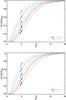 |
Fig. 2 Cumulative χ2 distributions when Td and βd are fixed in the filtering (solid red curve) or when they are left free (solid blue curve). Top panel: distribution for a dust-only filtering on a dust-only mock catalogue. Bottom panel: distribution for a dust + tSZ filtering on a dust + tSZ mock catalogue. In both cases (dust-only or dust + tSZ), fixing Td and βd leads to a χ2 distribution with seven degrees-of-freedom (corresponding to our seven maps), while leaving them free reduces the number of degrees-of-freedom to five. |
We next inject a mock catalogue with both dust and tSZ emission and re-extract the QSO signals using a dust + tSZ filter to compute the χ2. The results are shown in the bottom panel of Fig. 2.
Null test performed at fixed (Td = 25 K, βd = 2.5).
Fixing Td and βd to the input values also leads to a χ2 with seven d.o.f. Leaving the two dust parameters free lowers the χ2 to five d.o.f., as for the dust-only case. Although we are searching for an additional component in the data between the first and the second tests, the χ2 conserves 7/5 d.o.f. for (Td, βd) fixed/free respectively. This is because the correlations between our residuals are taken into account in the covariance matrix C [ ⟨ R ⟩ ] in Eq. (32). In other words, C [ ⟨ R ⟩ ] changes when considering the dust-only MMF or the dust + tSZ MMF, so the χ2 statistic defined in Eq. (32) does not depend on the number of components assumed for the MMF.
4.3. Extraction of simulated QSO
We first consider null tests where the signals are extracted at random positions in the Planck maps. Table 1 shows the output for three filters (dust, dust + tSZ, dust + synch) assuming fixed values of Td = 25 K and βd = 2.5 in the extraction. The output dust masses, SZ masses and synchrotron luminosities are compatible with zero, as expected, and the χ2 do not show any significant deviation from Student’s law with the expected seven d.o.f.
Results of the extraction on mock catalogs injected into the Planck maps are summarized in Table 2. The recovered dust masses, SZ masses, and synchrotron luminosities are marginalized over Td and βd as described in Sect. 3.5.
For the injected dust + tSZ catalogue, the dust + tSZ filter recovers a unbiased estimate of the input dust temperature and spectral index. The input dust mass and the halo mass from the tSZ are also recovered at S/N ~ 8 and S/N ~ 14. The dust mass recovered using the dust-only filter is biased by + 3.4σ due to contamination of the dust emission by the tSZ. The recovered dust spectral index is also biased by −3.7σ. Adopting the dust + synch filter leads to a significant detection of negative synchrotron luminosity at + 4.6σ, which mimics the tSZ effect at low frequencies.
The dust-only extraction provides a reduced χ2/ 5 value of 12.1, larger than the dust + tSZ value of 1.1, indicating that the dust + tSZ model must be preferred over the dust-only model. The dust + synch model provides a better χ2/ 5 than the dust-only case (4.0), but the significantly negative value for the synchrotron luminosity discards the model. The (Td,βd) contours for the three filters are displayed in Fig. 3. The dust + tSZ filter shows contours enclosing the input values while the two other filters are biased.
We also implemented the triple dust + tSZ + synch filter and applied it to the dust + tSZ simulation. The triple filter transforms part of the tSZ emission into a negative (i.e., unphysical) synchrotron emission, as shown in Table 2. It recovers biased Td, βd, and Mdust. The reduced χ2/ 5 increases with respect to the dust + tSZ filter, showing that the dust + tSZ fit must be preferred over the dust + tSZ + synch fit. We show in Sect. 5 that the triple filter exhibits the same behavior on the data. We will thus present our main results using the dust, the dust + tSZ, and the dust + synch filters, depending on the value of the reduced χ2/ 5.
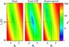 |
Fig. 3 Contours of χ2 for the mock QSO dust + tSZ catalogue using the dust, the dust + tSZ, and the dust + synch filters. The solid black line indicates the 1σ deviation from the minimal χ2 and the dotted black line the 2σ deviation. The horizontal and vertical dashed lines mark the position of the input Td and βd. |
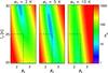 |
Fig. 4 Contours of χ2 for the mock QSO dust (σT = 5 K) + tSZ catalogue, obtained using the dust(σT = 2 K) + tSZ, the dust (σT = 5 K) + tSZ, and the dust (σT = 10 K) + tSZ filters. The solid black line indicates the 1σ deviation from the minimal χ2, and the dotted black line the 2σ deviation. The horizontal and vertical dashed lines mark the position of the input Td and βd. |
4.4. Possible systematics due to the dust characteristics
We test the sensitivity of the extraction method to improper modeling of the dust by injecting mock QSOs with a dust temperature following a Gaussian distribution, described in Sect. 4.1, and then recovering the parameters with the different MMF. Results are shown in the bottom part of Table 2. The dust (σT = xK) + tSZ filters are a dust + tSZ filter for which a Gaussian scatter of x Kelvin in the dust temperature is added. As expected, the dust (σT = 5 K) + tSZ filter provides an unbiased estimate of the parameters. The derived dust and SZ masses are not very sensitive to the dispersion in the dust temperature: the dust + tSZ filter returns a satisfactory estimate of the two quantities. However, for this latter filter the recovered dust parameters Td and βd are significantly biased. This sensitivity is illustrated in Fig. 4 displaying the (Td, βd) contours for the three last filters of Table 2.
5. Results
We apply the method described in Sect. 3 to the real Planck data. In Sect. 5.1, we show the average total flux of the QSO sample across the Planck channels. We then estimate the contribution of the various components in Sects. 5.2 (dust), 5.3 (synchrotron), and 5.4 (hot gas).
5.1. The QSO signal at Planck frequencies
We first estimate the mean flux density,  , of the 291 165 QSOs selected in Sect. 2.1 by averaging the individual flux densities in each band as extracted with a single frequency matched filter centered on the QSO positions. The average total flux is shown as the black diamonds in Fig. 5 (main panel and inset). It is strictly positive in all Planck bands above 100 GHz, and positive but compatible with zero at 70 GHz. The signal continuously increases from the lowest to the highest frequencies: emission in the direction of the QSO is dominated by dust. Since none of the frequencies below 217 GHz presents a negative flux, there is no obvious indication of strong tSZ emission.
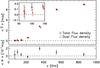 |
Fig. 5 Average flux density for the QSO population across Planck channels (black diamonds), and dust signal estimated with the dust-only filter (red triangles) for Td and βd at the minimum χ2. The bottom panel shows the average residuals. |
Using the dust-only MMF with Td and βd adjusted to minimize the χ2 defined in Eq. (32) (Td = 18.7 K, βd = 2.79), we compute the mean dust flux density and plot the resulting mean dust spectrum as the red triangles in Fig. 5. Dust accounts for essentially all the observed signal. The residual (difference between the black diamonds and the red triangles) is shown in the bottom panel of the figure, and is consistent with zero except at 353 GHz. This deviation explains why the reduced χ2/ 5 highlighted in the first gray line of Table 3 is not good (χ2/ 5 = 5.2).
By marginalizing over Td and βd, we obtain an average dust mass, 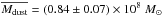 . This value is ~25 times smaller than the estimated dust mass in optically-selected clusters, around 2 × 10⁹M⊙ (Gutiérrez & López-Corredoira 2014). It is also five times smaller than the lowest estimated QSO dust mass of the Beelen et al. (2006) sample. We note, however, that our average mass is dominated by low redshift objects (z ~ 0.5), as shown in Fig. 7, while the QSO sample studied in Beelen et al. (2006) resides at higher redshift.
The recovered dust mass also depends strongly on the assumed value for Td and βd. If we fix βd = 1.6, as in Beelen et al. (2006), we find 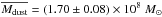 , in better agreement with the above-cited study, but the χ2/ 5 increases to 16.3, as shown in Table 3. This result demonstrates that the bulk of the BOSS QSO population contains significantly less dust than QSOs examined in these previous studies.
Average properties of different QSO samples in Planck data, marginalized over Td and βd (see Sect. 3.5), except for line 1 and 6 marginalized over Td only, βd being fixed to 1.6 as in Beelen et al. (2006).
For the dust temperature, we find a marginalized Td = 19.1 ± 0.8 K, close to the dust temperature of normal galaxies (e.g., Clemens et al. 2013). This is significantly lower than the temperature found by Beelen et al. (2006) and Dai et al. (2012), ranging between 33 and 55 K, and 18.1 and 79.7 K respectively. We note that Dai et al. (2012) use the two component model from Blain et al. (2003) with βd = 2, and Beelen et al. (2006) fix βd = 1.6 for the majority of their QSOs. We find βd = 2.71 ± 0.13, significantly higher than these values. When fixing βd = 1.6 in our analysis, our result moves along the degeneracy line in the (Td, βd)-plane to reach Td = 28.2 ± 0.5 K, in better agreement with the values published in the previously mentioned analyses. Restricting this test to high redshift QSOs leaves our conclusions unchanged (line 6 of Table 3).
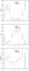 |
Fig. 6 Top panel: average Td as a function of redshift z. Middle panel: average βd as a function of redshift z. There is a clear evolution between the low-z (z< 1.5) , high-temperature and low-β and the high-z, low-temperature and high-β QSO populations. Bottom panel: average dust |

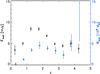 |
Fig. 7 Average dust flux density after marginalization over Td and βd (black diamonds) as a function of redshift z. The corresponding dust mass is shown as blue triangles (Eq. (20)). The extraction is achieved using the dust-only filter. |
5.2. Redshift dependence of the dust properties
In order to adapt the MMF to a possible variation of the QSO dust properties across redshift, we divide our QSO sample into nine regular bins of size Δz = 0.5, shown as the vertical dashed lines in Fig. 1. We include in the last bin the QSOs with 4 <z< 5 because there are not enough statistics to fill a tenth bin.
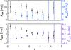 |
Fig. 8 Top panel: average dust flux density (black diamonds) for QSOs with a radio counterpart in the FIRST catalogue. The signal is extracted with the dust + synch filter and marginalized over Td and βd. The corresponding dust mass is shown as the blue triangles. Bottom panel: average synchrotron flux density at 100 GHz observed frequency (black diamonds) and the corresponding monochromatic luminosity (magenta triangles). |
We minimize the χ2 for each bin individually and plot the value for the combination  in Fig. 6. This quantity follows the degeneracy line for the dust parameters. There is no evidence for significant evolution across redshift between z = 0 and 2. For z> 2, increases with redshift. If we suppose that βd remains constant, this implies that the dust was hotter at high redshift and cooled until z = 2 before stabilizing at the current values.
The dust flux density extracted using the dust-only MMF is shown in Fig. 7 as the black diamonds. It varies with redshift, increasing from z = 0 to z = 2 (~8 mJy within R500 at 857 GHz) and decreasing with redshift for z> 2. The corresponding dust mass (Eq. (20)) is shown by the blue diamonds and follows the same trend as the flux density, reaching a maximum of ~5 × 10⁸M⊙ at z ~ 2. This is of the same order as dust masses determined from high signal-to-noise observations of individual QSOs (e.g., Beelen et al. 2006; Wang et al. 2007).
The IR luminosity, or equivalently the dust mass (Eq. (20)), is a tracer of star formation, and it is remarkable that the dust mass evolution in Fig. 7 follows that of the general star formation rate with a peak around z ~ 2 (see, e.g., Fig. 9 in Madau & Dickinson 2014). The accretion rate onto AGN SMBHs follows the same trend (Hopkins et al. 2007; Shankar et al. 2009; Aird et al. 2010; Delvecchio et al. 2014). This is strong evidence that star formation in QSO environments is typical of the general galaxy population, and also that it is linked to the QSO central engines. Our result clearly shows this trend for a large, representative sample of QSOs, and is consistent with the study by Wang et al. (2015) of the correlation between QSOs and Herschel measurements of the cosmic infrared background.
Table 3 also contains results for the dust + tSZ, dust + synch, and the dust + tSZ + synch filters on the full QSO population (0.1 <z< 6.5). All three of the multiple component filters increase the χ2 with respect to the dust-only filter.
5.3. Synchrotron emission
We now select only QSOs with at least one FIRST3 radio source counterpart at 1.4 GHz using the FIRST_MATCH keyword in the DR12 catalogue (FIRST_MATCH = 1). This provides a sub-catalogue of 9983 QSOs. Applying the dust + synch filter to this sub-catalogue using the same redshift binning, we plot the average dust and synchrotron flux densities,  and
and  , in Fig. 8. Dust emission from the sub-catalogue is compatible with that of the full catalogue, although with larger uncertainties due to the smaller sample (blue diamonds).
This population of radio-loud QSOs exhibits strong synchrotron emission, as shown in the lower panel. The monochromatic synchrotron luminosity (green diamonds) increases from 0 to reach 0.2 L⊙ Hz-1 at the higher redshifts; We note that this is the luminosity at the rest-frame frequency 100 GHz, assuming our power-law in Eq. (21).
Figure 9 compares the synchrotron emission determined from Planck (expressed at 100 GHz) to the FIRST measurements at 1.4 GHz. For this comparison, we bin-average the FIRST signal with the same MMF weights used to extract the synchrotron signal. The emission seen by Planck steadily decreases with redshift relative to the signal measured by FIRST, demonstrating a variation in synchrotron index with redshift.
We show the effective spectral index (for an assumed power law) between FIRST and Planck in Fig. 10. The spectrum is quite flat at low redshift with values for the spectral index that are much smaller than our adopted value of 0.7. However, these are values describing the emission over a very large frequency range, while our adopted value is assumed to describe the emission around 100 GHz.
We also see that the effective spectral index steepens with redshift. This could be due to evolution intrinsic to the sources, or more simply the effect of curvature in the synchrotron spectrum. It is important to note in this light that although our synchrotron luminosity measurements (Eq. (21)) are referenced to 100 GHz rest-frame, assuming our adopted power law, the effective index shown in Fig. 10 is taken between the observed 1.4 and 100 GHz bands. In other words, it is the effective index between rest-frame frequencies of 1.4(1 + z) and 100(1 + z) GHz. The apparent evolution with redshift in the figure could therefore be steepening in the synchrotron emission with frequency that would be expected given the greater energy loss of the higher energy electrons contributing to the signal as we move up in rest-frame frequency.
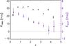 |
Fig. 9 Average FIRST flux density at 1.4 GHz observed frequency compared to the average synchrotron flux density at 100 GHz observed frequency as a function of redshift z. The magenta triangles correspond to the black diamonds in the bottom panel of Fig. 8. |
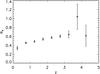 |
Fig. 10 Effective spectral index of power law in frequency between 1.4 GHz (FIRST) and 100 GHz (Planck) observation frequencies. |
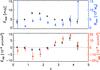 |
Fig. 11 Top panel: average dust flux density (black diamonds) of the radio-quite QSO subsample, i.e., without a radio counterpart in the FIRST catalogue. The signal is obtained with the dust + tSZ filter and is marginalized over Td and βd. The corresponding dust mass is shown by the blue triangles. Bottom panel: average Compton parameter (black diamonds) and corresponding integrated Compton parameter (red triangles) as a function of redshift. |
5.4. Hot halo gas
The strong synchrotron emission of QSOs with FIRST counterparts complicates extraction of the tSZ signal from the hot gas in the host halo. We therefore construct a sub-sample without FIRST counterparts (FIRST_MATCH = 0) of 252 888 QSOs and apply the dust + tSZ filter. Results are shown in Fig. 11, and summarized in the bottom segment of Table 3 for this and other filters.
Average properties from a SZ filtering for several samples of QSO.
Average properties of the 2.5 <z< 4 QSO sample without FIRST counterpart for three filtering sizes θs.
Applied to the same redshift range, the other filters yield larger χ2 values. In particular, the dust + synch and dust + tSZ + synch filters show the same behavior as on simulations: they convert part of the tSZ signal into negative synchrotron luminosity. The dust(σT = x K) + tSZ filters presented in Sect. 4.4 also increase the χ2, favoring a low scatter in the dust temperature.
The filter does not detect the tSZ effect at z< 2.5. The tSZ signal at z< 1.5 is slightly negative at ~2σ, pointing towards a possible contamination of the extracted signal at low z by a weak synchrotron emission. The filter does show a clear signal rising with redshift over the range 2.5 <z< 4. The global significance of the signal in the latter redshift range is 7.4σ when expressed in terms of the population mean,  .
.
The dust + tSZ + synch filter applied on the radio-loud sub-catalogue, i.e., with at least one FIRST source (third segment of Table 3), provides a slightly better fit (χ2/ 5 = 0.3) than the dust + synch filter (χ2/ 5 = 0.4) over the 2.5 <z< 4 range. The recovered SZ signal remains compatible with the value derived from the radio-quiet sub-catalogue, but the uncertainties are large with the signal appearing at only 1.5σ.
When applying the tSZ-only filter to the 2.5 <z< 4 population, we find SZ-based masses that are twice as large as the mass provided by the dust + tSZ filter; the fit, however, is quite bad at χ2/ 7 > 100. (We note that there are seven degrees-of-freedom in this case because the dust temperature and emissivity do not come into play.) This simply reflects the fact that a tSZ-only signal is a poor description of the spectrum of the source. Details of these results are given in Table 4.
We stacked the ROSAT All-Sky Survey maps4 of the radio-quiet QSO sub-sample to find a significant signal, corresponding to a population mean luminosity of L500 = (3.30 ± 0.30) × 1044erg / s in the [0.1–2.4] keV band, the error taken as the standard deviation of the stacked maps. Pratt et al. (2009) established a power-law scaling relation between X-ray luminosity and halo mass based on analysis of a representative sample of X-ray galaxy clusters employing Bivariate Correlated Errors and intrinsic Scatter estimators with a minimization of the residuals in X-ray luminosity (BCES (YlX)). If we adopt their Malmquist-bias corrected relation between L500, in this energy band, and mass (line 6 of their Table B.2), we infer a mean halo mass of M500 = 5.87 × 10¹³M⊙. This is 2.3 times higher than our SZ-based mass; alternatively, it implies an expected  , or 4.7 times larger than our measurement. In other words, the tSZ and X-ray signals do not follow the empirical relation for thermal halo gas emission seen at low redshift (Planck Collaboration XI 2011). This is not a surprise given that we expect a non-negligible contribution to the X-ray emission from the central engine of the QSO itself.
5.5. Sensitivity to the assumed size θs
We fix θs = 0.27 arcmin throughout our analysis. The value corresponds to a halo mass of M500 = 1013M⊙ at z = 2. To test the robustness of our results to this assumption, we fix alternatively the size to θs = 0.12 and θs = 0.57 arcmin, corresponding to halos of mass M500 = 1012M⊙ and M500 = 1014M⊙, respectively, at z = 2. Results are shown in Table 5. Changing the filtering scale slightly increases the χ2, and only weakly impacts the derived parameters (<0.5σ), leaving our results essentially unchanged.
6. Discussion
Submillimeter observations are a valuable source of information on the physical conditions in QSO environments because they probe star formation in and around the hosts and energy injection into the surrounding medium by the SMBHs. Due to atmospheric absorption, this waveband is however difficult to access from the ground, and this has limited studies to relatively small samples of several tens of objects (Omont et al. 2001, 2013; Isaak et al. 2002; Priddey et al. 2003; Beelen et al. 2006; Wang et al. 2007).
The space-based platforms WMAP, Planck and Herschel now open this window for much more extensive studies. Taking advantage of Planck’s all-sky and wide-frequency coverage, we have determined several mean characterstics of the QSO population through binning measurements of dust, synchrotron and tSZ signals from the very large BOSS QSO sample.
6.1. Dust emission
We find that the QSO spectrum is dominated by graybody dust emission with a temperature of Td = 19.1 ± 0.8 K and an emissivity spectral index of βd = 2.71 ± 0.13 when averaged over the entire sample spanning the full redshift range, 0.1 <z< 5; these are the one-dimensional marginalized constraints for the dust-only filter that gives the best χ2 (see Table 3). While there is no clear evidence that these quantities evolve with redshift at z< 2, there is a rise at higher redshifts in the product  , describing the degeneracy direction, at higher redshifts (Fig. 6).
Curiously, the temperature is notably lower than found in ground-based observations of high-redshift quasars, which find temperatures of 40–50 K, while our value is more typical of ordinary galaxies like the Milk Way. Our dust emissivity index is significantly steeper than the values of 1–2 for normal Galactic dust, and should be compared to the value of 1.6 found in the ground-based surveys. It is notably steeper than the limiting case of β = 2 for ideal insulators and conductors far from a resonance. These characteristics remain in the other sub-samples and component filters summarized in Table 3, apart the unusual behaviour of the radio-loud sub-sample with FIRST counterparts. Fixing βd = 1.6, we obtain a somewhat higher mean temperature, Tdust = 28.2 ± 0.5 K, but at the cost of a much worse spectral fit according to the large increase in χ2 (see Table 3).
We calculate dust mass using the simple prescription of Eq. (20), which can also be viewed as a measure of far-IR luminosity. An important result is our finding that the dust mass, a tracer of local star formation, evolves with redshift in the same way as the global cosmic star formation rate, peaking at z ~ 2 (see e.g. Fig. 9 in Madau & Dickinson 2014). Star formation in QSO environments apparently does not distinguish itself from others. It is also known, from measures of AGN luminosity functions, that the SMBH accretion rate follows the same evolutionary track (Hopkins et al. 2007; Shankar et al. 2009; Aird et al. 2010; Delvecchio et al. 2014).
6.2. Synchrotron emission
A subsample of our QSOs are radio loud with counterparts at 1.4 GHz in the FIRST catalogue. We detect synchrotron emission from this subsample with an monochromatic luminosity, referenced to rest frame frequency 100 GHz (adopting our power-law of Eq. (21)), increasing with redshift between z = 0 and z = 3. Comparing the FIRST and Planck flux densities, we find an effective spectral index between the two corresponding rest-frame frequencies that increases with redshift from αs = 0.3 to αs = 0.7. This steepening is likely the result of curvature in the spectrum as we observe progressively higher rest-frame frequencies.
6.3. tSZ and feedback
Restricting analysis to the radio-quite sub-sample, we detect the tSZ effect (with the dust + tSZ filter) at S/N ~ 7.4 over the redshift range 2.5 <z< 4, with an integrated Compton-y parameter of  (one-dimensional, marginalized over dust properties). We do not, however, find evidence of tSZ signal at the lower redshifts. At z< 1.5, we obtain a mean value of
  arcmin2, which we convert simply into an upper limit at two sigma above zero as
  (38)Similarly, we find an upper limit at z< 2.5 of
  (39)even stronger, as expected given the behaviour seen in Fig. 11.
Ruan et al. (2015) recently reported a detection of the tSZ signal by stacking the Hill & Spergel (2014) tSZ map, constructed from the Planck frequency maps, on 26 686 spectroscopic DR7 QSOs. For their low redshift bin at z< 1.5, they find  arcmin2, quoted in terms of the Compton-y parameter integrated along the line-of-sight cylinder. The conversion factor between the cylindrical and spherical integrated Compton-y parameters for our adopted profile is
  , which translates the upper limit of Eq. (38) to
  arcmin2 (2σ), well below their detection level.
One possible explanation for the difference is dust contamination. Ruan et al. (2015) took particular pains to correct for any contamination by dust in the tSZ map. Our filters directly measure the individual local signals from dust and tSZ, as well as any covariance between them, allowing us to separate and marginalize over the dust influence when quoting our tSZ signal strengths. The importance of separating out the dust signal is easily appreciated from the results of applying the tSZ-only filter given in Table 4. Contamination by dust in the tSZ-only filter can produce tSZ signals ~3 times larger.
The tSZ signal directly measures the thermal energy stored in diffuse ionized gas in the QSO environment. We expect a signal from the intra-halo gas at the virial temperature of the QSO host halo, and there may be additional heating powered by feedback from the SMBH. Chatterjee et al. (2010) and Ruan et al. (2015) both interpreted their tSZ signals as evidence for feedback into the surrounding gas.
To look for this, we estimate the tSZ signal expected from intra-halo gas using the scaling relation between halo mass and tSZ signal in Eq. (23). We first establish a mean mass scale for the sample of 77 655 QSOs in 2.5 <z< 4 over the 14 555 sq. deg. SDSS footprint. Using the Tinker et al. (2008) mass function, we find the lower mass bound above which there are as many predicted halos as observed QSOs in this redshift range and for this sky area. We then calculate the mean mass by integrating over the mass function above this mass limit and over this redshift range. This gives us an estimate of the maximum mean mass characterizing the sample; QSOs could be hosted by lower mass halos if the QSO selection function is not 100% complete, as is most certainly the case.
We find a mean halo mass of M500,true = 2.18 × 10¹³M⊙, a value in reasonable agreement with Richardson et al. (2012), who found a QSO halo mass  at z ~ 3.2 for the SDSS sample. Our characteristic mass corresponds to a predicted tSZ signal of Y500 = 8.47(1 − b)1.78 × 10⁻⁶ arcmin2, only one sigma below our measured signal of Y500 = (10.02 ± 1.34) × 10-6 arcmin2 if b = 0. This would not leave much room for additional heating by feedback. With the higher mass bias values suggested by Planck’s cluster counts, e.g., (1 − b) = 0.6, we instead have Y500 = 3.4 × 10⁻⁶ arcmin2, implying that ~60% of the gas’s thermal energy is generated by feedback.
X-ray emission from the hot gas is also expected. Stacking the RASS maps at the QSO position, we find a luminosity L500 = (3.30 ± 0.30) × 1044 erg / s in the [0.1–2.4] keV band. The tSZ – X-ray luminosity scaling relation established by Planck Collaboration X (2011) says that this should correspond to an SZ signal of  , much higher than our actual tSZ measurement, a conclusion that is independent of the mass bias.
The cluster halo gas scaling relations appear therefore to be violated in the QSO environment. This could be due to feedback from the QSO SMBH. It is likely that X-ray emission from the QSO itself also affects our X-ray measurements. Moreover, we are extrapolating the relation to redshifts much higher than those used to establish its validity. The redshift evolution of these relations is in fact not well known, and we have adopted self-similar evolution as a reasonable assumption given the lack of empirical constraints. Measurements of these relations on non-QSO systems at the same redshifts would provide a valuable comparison sample to judge if the QSO’s activity is in fact responsible for violating the scaling relations.
Finally, we note that interpretation of the measured tSZ signal is also clouded by possible contribution from gas in structures correlated with the QSO halos and falling with the relatively large effective beam of Planck, as suggested by Cen & Safarzadeh (2015). We leave careful modeling of this effect to future work.
7. Conclusion
Planck’s coverage of the SDSS survey area gives us the opportunity for in-depth study of quasar environments through submillimeter observations of optically selected QSOs. This spectral band provides valuable information on star formation and energy production by the QSO central engines. Filtering Planck’s seven spectral bands from 70–857 GHz with multi-component MMFs, we have measured dust, synchrotron and tSZ signals from the large BOSS QSO sample spanning redshifts out to 0.1 <z< 5. While measurements of individual QSOs are well below Planck’s sensitivity, the MMFs enable us to determine the population’s mean properties as a function of redshift.
Dust emission dominates the average QSO spectrum, and its evolution with redshift suggests that star formation in QSO environments follows the general cosmic star formation rate with a peak at z ~ 2. We did not detect a tSZ signal from QSOs at z< 2.5, but did find a signal at higher redshifts. The signal is clearly seen out to z ~ 4, the highest redshift to which the tSZ signal has been measured to date. A non-negligible fraction of the gas’s thermal energy could be supplied by QSO feedback, but interpretation is difficult because of modeling uncertainties associated with halo gas scaling relations. Finally, we observe synchrotron emission from a radio-loud sub-sample at rest-frame frequencies ν> 100 GHz and whose luminosity rises monotonically with redshift.
These results are based on a large sample of nearly 300 000 BOSS spectroscopic QSOs falling outside of the Planck mask. Our findings present a fresh and representative view of the average properties characterizing the QSO population.
Acknowledgments
Some of the results in this paper have been derived using the HEALPix (Górski et al. 2005) package. Part of this research was carried out at the Jet Propulsion Laboratory, California Institute of Technology, under a contract with the National Aeronautics and Space Administration. We thank T. Marriage for helpful discussions.
References
- Aird, J., Nandra, K., Laird, E. S., et al. 2010, MNRAS, 401, 2531 [NASA ADS] [CrossRef] [Google Scholar]
- Alam, S., Albareti, F. D., Allen de Prieto, C., et al. 2015, ApJS, 219, 12 [NASA ADS] [CrossRef] [Google Scholar]
- Arnaud, M., Pratt, G. W., Piffaretti, R., et al. 2010, A&A, 517, A92 [NASA ADS] [CrossRef] [EDP Sciences] [Google Scholar]
- Beelen, A., Cox, P., Benford, D. J., et al. 2006, ApJ, 642, 694 [NASA ADS] [CrossRef] [Google Scholar]
- Bennett, C. L., Bay, M., Halpern, M., et al. 2003, ApJ, 583, 1 [NASA ADS] [CrossRef] [Google Scholar]
- Bersanelli, M., Mandolesi, N., Butler, R. C., et al. 2010, A&A, 520, A4 [NASA ADS] [CrossRef] [EDP Sciences] [Google Scholar]
- Birkinshaw, M. 1999, Phys. Rep., 310, 97 [NASA ADS] [CrossRef] [Google Scholar]
- Blain, A. W., Barnard, V. E., & Chapman, S. C. 2003, MNRAS, 338, 733 [NASA ADS] [CrossRef] [Google Scholar]
- Blanchard, A., Valls-Gabaud, D., & Mamon, G. A. 1992, A&A, 264, 365 [NASA ADS] [Google Scholar]
- Bower, R. G., Benson, A. J., Malbon, R., et al. 2006, MNRAS, 370, 645 [NASA ADS] [CrossRef] [Google Scholar]
- Busca, N. G., Delubac, T., Rich, J., et al. 2013, A&A, 552, A96 [NASA ADS] [CrossRef] [EDP Sciences] [Google Scholar]
- Carlstrom, J. E., Holder, G. P., & Reese, E. D. 2002, ARA&A, 40, 643 [NASA ADS] [CrossRef] [Google Scholar]
- Cen, R., & Safarzadeh, M. 2015, ApJ, 809, L32 [NASA ADS] [CrossRef] [Google Scholar]
- Chatterjee, S., Ho, S., Newman, J. A., & Kosowsky, A. 2010, ApJ, 720, 299 [NASA ADS] [CrossRef] [Google Scholar]
- Clemens, M. S., Negrello, M., De Zotti, G., et al. 2013, MNRAS, 433, 695 [NASA ADS] [CrossRef] [Google Scholar]
- Condon, J. J. 1992, ARA&A, 30, 575 [NASA ADS] [CrossRef] [MathSciNet] [Google Scholar]
- Crichton, D., Gralla, M. B., Hall, K., et al. 2015, MNRAS, in press [arXiv:1510.05656] [Google Scholar]
- Croom, S. M., Shanks, T., Boyle, B. J., et al. 2001, MNRAS, 325, 483 [NASA ADS] [CrossRef] [Google Scholar]
- Croton, D. J., Springel, V., White, S. D. M., et al. 2006, MNRAS, 365, 11 [NASA ADS] [CrossRef] [Google Scholar]
- Dai, Y. S., Bergeron, J., Elvis, M., et al. 2012, ApJ, 753, 33 [NASA ADS] [CrossRef] [Google Scholar]
- Dawson, K. S., Schlegel, D. J., Ahn, C. P., et al. 2013, AJ, 145, 10 [Google Scholar]
- Delubac, T., Bautista, J. E., Busca, N. G., et al. 2015, A&A, 574, A59 [NASA ADS] [CrossRef] [EDP Sciences] [Google Scholar]
- Delvecchio, I., Gruppioni, C., Pozzi, F., et al. 2014, MNRAS, 439, 2736 [NASA ADS] [CrossRef] [Google Scholar]
- Eisenstein, D. J., Weinberg, D. H., Agol, E., et al. 2011, AJ, 142, 72 [Google Scholar]
- Fabian, A. C. 2012, ARA&A, 50, 455 [NASA ADS] [CrossRef] [Google Scholar]
- Ferrarese, L., & Merritt, D. 2000, ApJ, 539, L9 [NASA ADS] [CrossRef] [Google Scholar]
- Gebhardt, K., Bender, R., Bower, G., et al. 2000, ApJ, 539, L13 [NASA ADS] [CrossRef] [Google Scholar]
- Górski, K. M., Hivon, E., Banday, A. J., et al. 2005, ApJ, 622, 759 [NASA ADS] [CrossRef] [Google Scholar]
- Gralla, M. B., Crichton, D., Marriage, T. A., et al. 2014, MNRAS, 445, 460 [NASA ADS] [CrossRef] [Google Scholar]
- Gutiérrez, C. M., & López-Corredoira, M. 2014, A&A, 571, A66 [NASA ADS] [CrossRef] [EDP Sciences] [Google Scholar]
- Haehnelt, M. G., & Tegmark, M. 1996, MNRAS, 279, 545 [NASA ADS] [CrossRef] [Google Scholar]
- Herranz, D., Sanz, J. L., Hobson, M. P., et al. 2002, MNRAS, 336, 1057 [NASA ADS] [CrossRef] [Google Scholar]
- Hill, J. C., & Spergel, D. N. 2014, J. Cosmol. Astropart. Phys., 2, 30 [Google Scholar]
- Hopkins, P. F., Richards, G. T., & Hernquist, L. 2007, ApJ, 654, 731 [NASA ADS] [CrossRef] [Google Scholar]
- Isaak, K. G., Priddey, R. S., McMahon, R. G., et al. 2002, MNRAS, 329, 149 [NASA ADS] [CrossRef] [Google Scholar]
- Kormendy, J., & Richstone, D. 1995, ARA&A, 33, 581 [NASA ADS] [CrossRef] [Google Scholar]
- Lamarre, J., Puget, J., Ade, P. A. R., et al. 2010, A&A, 520, A9 [NASA ADS] [CrossRef] [EDP Sciences] [Google Scholar]
- Lynden-Bell, D. 1969, Nature, 223, 690 [NASA ADS] [CrossRef] [Google Scholar]
- Madau, P., & Dickinson, M. 2014, ARA&A, 52, 415 [NASA ADS] [CrossRef] [Google Scholar]
- McNamara, B. R., & Nulsen, P. E. J. 2007, ARA&A, 45, 117 [NASA ADS] [CrossRef] [MathSciNet] [Google Scholar]
- Melin, J.-B., Bartlett, J. G., & Delabrouille, J. 2006, A&A, 459, 341 [NASA ADS] [CrossRef] [EDP Sciences] [Google Scholar]
- Melin, J.-B., Bartlett, J. G., Delabrouille, J., et al. 2011, A&A, 525, A139 [NASA ADS] [CrossRef] [EDP Sciences] [Google Scholar]
- Mennella, A., Butler, R. C., Curto, A., et al. 2011, A&A, 536, A3 [NASA ADS] [CrossRef] [EDP Sciences] [Google Scholar]
- Nandra, K., Georgakakis, A., Willmer, C. N. A., et al. 2007, ApJ, 660, L11 [NASA ADS] [CrossRef] [Google Scholar]
- Omont, A., Cox, P., Bertoldi, F., et al. 2001, A&A, 374, 371 [NASA ADS] [CrossRef] [EDP Sciences] [Google Scholar]
- Omont, A., Beelen, A., Bertoldi, F., et al. 2003, A&A, 398, 857 [NASA ADS] [CrossRef] [EDP Sciences] [Google Scholar]
- Omont, A., Willott, C. J., Beelen, A., et al. 2013, A&A, 552, A43 [NASA ADS] [CrossRef] [EDP Sciences] [Google Scholar]
- Palanque-Delabrouille, N., Yeche, C., Myers, A. D., et al. 2011, A&A, 530, A122 [NASA ADS] [CrossRef] [EDP Sciences] [Google Scholar]
- Pâris, I., Petitjean, P., Aubourg, É., et al. 2012, A&A, 548, A66 [NASA ADS] [CrossRef] [EDP Sciences] [Google Scholar]
- Peterson, B. M. 1997, An Introduction to Active Galactic Nuclei (Cambridge, New York: Cambridge University Press) [Google Scholar]
- Planck Collaboration I. 2011, A&A, 536, A1 [NASA ADS] [CrossRef] [EDP Sciences] [Google Scholar]
- Planck Collaboration VIII. 2011, A&A, 536, A8 [NASA ADS] [CrossRef] [EDP Sciences] [Google Scholar]
- Planck Collaboration XI. 2011, A&A, 536, A11 [NASA ADS] [CrossRef] [EDP Sciences] [Google Scholar]
- Planck Collaboration X. 2011, A&A, 536, A10 [NASA ADS] [CrossRef] [EDP Sciences] [Google Scholar]
- Planck Collaboration XII. 2011, A&A, 536, A12 [NASA ADS] [CrossRef] [EDP Sciences] [Google Scholar]
- Planck Collaboration Int. XI. 2013, A&A, 557, A52 [NASA ADS] [CrossRef] [EDP Sciences] [Google Scholar]
- Planck Collaboration Int. XIII. 2014, A&A, 561, A97 [NASA ADS] [CrossRef] [EDP Sciences] [Google Scholar]
- Planck Collaboration XX. 2014, A&A, 571, A20 [NASA ADS] [CrossRef] [EDP Sciences] [Google Scholar]
- Planck Collaboration XXIX. 2014, A&A, 571, A29 [NASA ADS] [CrossRef] [EDP Sciences] [Google Scholar]
- Planck Collaboration I. 2015, ArXiv e-prints [arXiv:1502.01582] [Google Scholar]
- Planck Collaboration VI. 2015, ArXiv e-prints [arXiv:1502.01585] [Google Scholar]
- Planck Collaboration VIII. 2015, ArXiv e-prints [arXiv:1502.01587] [Google Scholar]
- Planck Collaboration XIII. 2015, ArXiv e-prints [arXiv:1502.01589] [Google Scholar]
- Planck Collaboration XXIV. 2015, ArXiv e-prints [arXiv:1502.01597] [Google Scholar]
- Planck Collaboration XXVII. 2015, ArXiv e-prints [arXiv:1502.01598] [Google Scholar]
- Planck HFI Core Team IV. 2011, A&A, 536, A4 [NASA ADS] [CrossRef] [EDP Sciences] [Google Scholar]
- Pratt, G. W., Croston, J. H., Arnaud, M., & Böhringer, H. 2009, A&A, 498, 361 [NASA ADS] [CrossRef] [EDP Sciences] [Google Scholar]
- Priddey, R. S., Isaak, K. G., McMahon, R. G., Robson, E. I., & Pearson, C. P. 2003, MNRAS, 344, L74 [NASA ADS] [CrossRef] [Google Scholar]
- Rees, M. J. 1984, ARA&A, 22, 471 [NASA ADS] [CrossRef] [Google Scholar]
- Richardson, J., Zheng, Z., Chatterjee, S., Nagai, D., & Shen, Y. 2012, ApJ, 755, 30 [NASA ADS] [CrossRef] [Google Scholar]
- Ross, N. P., Myers, A. D., Sheldon, E. S., et al. 2012, ApJS, 199, 3 [NASA ADS] [CrossRef] [Google Scholar]
- Ruan, J. J., McQuinn, M., & Anderson, S. F. 2015, ApJ, 802, 135 [NASA ADS] [CrossRef] [Google Scholar]
- Salpeter, E. E. 1964, ApJ, 140, 796 [CrossRef] [Google Scholar]
- Sanz, J. L., Herranz, D., & Martínez-Gónzalez, E. 2001, ApJ, 552, 484 [NASA ADS] [CrossRef] [Google Scholar]
- Shankar, F., Weinberg, D. H., & Miralda-Escudé, J. 2009, ApJ, 690, 20 [NASA ADS] [CrossRef] [Google Scholar]
- Silverman, J. D., Green, P. J., Barkhouse, W. A., et al. 2008, ApJ, 679, 118 [NASA ADS] [CrossRef] [Google Scholar]
- Somerville, R. S., Hopkins, P. F., Cox, T. J., Robertson, B. E., & Hernquist, L. 2008, MNRAS, 391, 481 [NASA ADS] [CrossRef] [Google Scholar]
- Sunyaev, R. A., & Zeldovich, Y. B. 1970, Comments Astrophys. Space Phys., 2, 66 [NASA ADS] [Google Scholar]
- Sunyaev, R. A., & Zeldovich, Y. B. 1972, Comments Astrophys. Space Phys., 4, 173 [NASA ADS] [EDP Sciences] [Google Scholar]
- Tauber, J. A., Mandolesi, N., Puget, J.-L., et al. 2010, A&A, 520, A1 [NASA ADS] [CrossRef] [EDP Sciences] [Google Scholar]
- Tinker, J., Kravtsov, A. V., Klypin, A., et al. 2008, ApJ, 688, 709 [NASA ADS] [CrossRef] [Google Scholar]
- Wang, L., Viero, M., Ross, N. P., et al. 2015, MNRAS, 449, 4476 [NASA ADS] [CrossRef] [Google Scholar]
- Wang, R., Carilli, C. L., Beelen, A., et al. 2007, AJ, 134, 617 [NASA ADS] [CrossRef] [Google Scholar]
- White, M., Myers, A. D., Ross, N. P., et al. 2012, MNRAS, 424, 933 [NASA ADS] [CrossRef] [Google Scholar]
- York, D. G., Adelman, J., Anderson, Jr., J. E., et al. 2000, AJ, 120, 1579 [Google Scholar]
All Tables
Average properties of different QSO samples in Planck data, marginalized over Td and βd (see Sect. 3.5), except for line 1 and 6 marginalized over Td only, βd being fixed to 1.6 as in Beelen et al. (2006).
Average properties of the 2.5 <z< 4 QSO sample without FIRST counterpart for three filtering sizes θs.
All Figures
|
Fig. 1 Redshift distribution of the BOSS DR12 QSO sample. The distribution presents two peaks, at z ~ 0.8 and z ~ 2.3, due to the QSO target selection process (see text). The regular binning used throughout this paper (Δz = 0.5) is shown as the vertical dotted lines. |
| In the text | |
|
Fig. 2 Cumulative χ2 distributions when Td and βd are fixed in the filtering (solid red curve) or when they are left free (solid blue curve). Top panel: distribution for a dust-only filtering on a dust-only mock catalogue. Bottom panel: distribution for a dust + tSZ filtering on a dust + tSZ mock catalogue. In both cases (dust-only or dust + tSZ), fixing Td and βd leads to a χ2 distribution with seven degrees-of-freedom (corresponding to our seven maps), while leaving them free reduces the number of degrees-of-freedom to five. |
| In the text | |
|
Fig. 3 Contours of χ2 for the mock QSO dust + tSZ catalogue using the dust, the dust + tSZ, and the dust + synch filters. The solid black line indicates the 1σ deviation from the minimal χ2 and the dotted black line the 2σ deviation. The horizontal and vertical dashed lines mark the position of the input Td and βd. |
| In the text | |
|
Fig. 4 Contours of χ2 for the mock QSO dust (σT = 5 K) + tSZ catalogue, obtained using the dust(σT = 2 K) + tSZ, the dust (σT = 5 K) + tSZ, and the dust (σT = 10 K) + tSZ filters. The solid black line indicates the 1σ deviation from the minimal χ2, and the dotted black line the 2σ deviation. The horizontal and vertical dashed lines mark the position of the input Td and βd. |
| In the text | |
|
Fig. 5 Average flux density for the QSO population across Planck channels (black diamonds), and dust signal estimated with the dust-only filter (red triangles) for Td and βd at the minimum χ2. The bottom panel shows the average residuals. |
| In the text | |
|
Fig. 6 Top panel: average Td as a function of redshift z. Middle panel: average βd as a function of redshift z. There is a clear evolution between the low-z (z< 1.5) , high-temperature and low-β and the high-z, low-temperature and high-β QSO populations. Bottom panel: average dust |
| In the text | |
|
Fig. 7 Average dust flux density after marginalization over Td and βd (black diamonds) as a function of redshift z. The corresponding dust mass is shown as blue triangles (Eq. (20)). The extraction is achieved using the dust-only filter. |
| In the text | |
|
Fig. 8 Top panel: average dust flux density (black diamonds) for QSOs with a radio counterpart in the FIRST catalogue. The signal is extracted with the dust + synch filter and marginalized over Td and βd. The corresponding dust mass is shown as the blue triangles. Bottom panel: average synchrotron flux density at 100 GHz observed frequency (black diamonds) and the corresponding monochromatic luminosity (magenta triangles). |
| In the text | |
|
Fig. 9 Average FIRST flux density at 1.4 GHz observed frequency compared to the average synchrotron flux density at 100 GHz observed frequency as a function of redshift z. The magenta triangles correspond to the black diamonds in the bottom panel of Fig. 8. |
| In the text | |
|
Fig. 10 Effective spectral index of power law in frequency between 1.4 GHz (FIRST) and 100 GHz (Planck) observation frequencies. |
| In the text | |
|
Fig. 11 Top panel: average dust flux density (black diamonds) of the radio-quite QSO subsample, i.e., without a radio counterpart in the FIRST catalogue. The signal is obtained with the dust + tSZ filter and is marginalized over Td and βd. The corresponding dust mass is shown by the blue triangles. Bottom panel: average Compton parameter (black diamonds) and corresponding integrated Compton parameter (red triangles) as a function of redshift. |
| In the text | |
Current usage metrics show cumulative count of Article Views (full-text article views including HTML views, PDF and ePub downloads, according to the available data) and Abstracts Views on Vision4Press platform.
Data correspond to usage on the plateform after 2015. The current usage metrics is available 48-96 hours after online publication and is updated daily on week days.
Initial download of the metrics may take a while.