| Issue |
A&A
Volume 588, April 2016
|
|
|---|---|---|
| Article Number | A107 | |
| Number of page(s) | 13 | |
| Section | Astronomical instrumentation | |
| DOI | https://doi.org/10.1051/0004-6361/201527313 | |
| Published online | 25 March 2016 | |
Comparison of absolute gain photometric calibration between Planck/HFI and Herschel/SPIRE at 545 and 857 GHz
1 Institut d’Astrophysique Spatiale (IAS), CNRS (UMR 8617), Université Paris-Sud 11, Bât. 121, 91405 Orsay, France
2 Aix Marseille Université, CNRS, LAM (Laboratoire d’Astrophysique de Marseille) UMR 7326, 13388 Marseille, France
e-mail: This email address is being protected from spambots. You need JavaScript enabled to view it.
3 Canadian Institute for Theoretical Astrophysics, University of Toronto, 60 St. George Street, Toronto, ON M5S 3H8, Canada
4 NASA Herschel Science Center, IPAC, 770 South Wilson Avenue, Pasadena, CA 91125, USA
5 European Space Astronomy Centre (ESAC)/ESA, Villanueva de la Canada, 28691 Madrid, Spain
6 APC, Université Paris 7 Denis Diderot, 10 rue Alice Domon et Léonie Duquet, 75205 Paris Cedex 13, France
7 CNRS, IRAP, 9 Av. Colonel Roche, BP 44346, 31028 Toulouse Cedex 4, France
8 Université de Toulouse, UPS-OMP, IRAP, 31028 Toulouse Cedex 4, France
9 Department of Physics, and Jet Propulsion Laboratory, California Institute of Technology, 4800 Oak Grove Drive, Pasadena, CA, USA
10 School of Physics and Astronomy, Cardiff University, Queens Buildings, The Parade, Cardiff CF24 3AA, UK
11 Department of Physics, Princeton University, Princeton, NJ 08544, USA
12 LESIA, Observatoire de Paris, CNRS, UPMC, Université Paris-Diderot, 5 place J. Janssen, 92195 Meudon, France
13 Laboratoire de l’Accélérateur Linéaire, Université Paris-Sud, CNRS/IN2P3, 91898 Orsay, France
Received: 5 September 2015
Accepted: 21 January 2016
Abstract
We compare the absolute gain photometric calibration of the Planck/HFI and Herschel/SPIRE instruments on diffuse emission. The absolute calibration of HFI and SPIRE each relies on planet flux measurements and comparison with theoretical far-infrared emission models of planetary atmospheres. We measure the photometric cross calibration between the instruments at two overlapping bands, 545 GHz/500 μm and 857 GHz/350 μm. The SPIRE maps used have been processed in the Herschel Interactive Processing Environment (Version 12) and the HFI data are from the 2015 Public Data Release 2. For our study we used 15 large fields observed with SPIRE, which cover a total of about 120 deg2. We have selected these fields carefully to provide high signal-to-noise ratio, avoid residual systematics in the SPIRE maps, and span a wide range of surface brightness. The HFI maps are bandpass-corrected to match the emission observed by the SPIRE bandpasses. The SPIRE maps are convolved to match the HFI beam and put on a common pixel grid. We measure the cross-calibration relative gain between the instruments using two methods in each field, pixel-to-pixel correlation and angular power spectrum measurements. The SPIRE/HFI relative gains are 1.047 (±0.0069) and 1.003 (±0.0080) at 545 and 857 GHz, respectively, indicating very good agreement between the instruments. These relative gains deviate from unity by much less than the uncertainty of the absolute extended emission calibration, which is about 6.4% and 9.5% for HFI and SPIRE, respectively, but the deviations are comparable to the values 1.4% and 5.5% for HFI and SPIRE if the uncertainty from models of the common calibrator can be discounted. Of the 5.5% uncertainty for SPIRE, 4% arises from the uncertainty of the effective beam solid angle, which impacts the adopted SPIRE point source to extended source unit conversion factor, highlighting that as a focus for refinement.
Key words: methods: data analysis
© ESO, 2016
1. Introduction
The Planck1 and Herschel2 satellites have an interconnected history, including their launch together in 2009. Although operating with different scientific goals across many frequencies, Planck and Herschel have in common two very similar passbands, 545 GHz/500 μm and 857 GHz/350 μm. This redundancy is very important for complementary studies. For example, the combination of Planck large-scale and Herschel small-scale observations is valuable to the study of the cosmic infrared background anisotropies (e.g., Planck Collaboration XVIII 2011; Viero et al. 2013) and to understanding the interplay between interstellar medium structures and their environment (e.g., Planck Collaboration XXII 2011; Juvela et al. 2011). With the 2015 public data release 2 (PR2) of the Planck data and the growing public availability of processed Herschel observations, this is an opportune time to address the important question of the compatibility of measurements carried out by both instruments.
The Planck High Frequency Instrument (HFI, Planck Collaboration VI 2014) is composed of a set of 52 bolometers observing the sky at six frequencies (100, 143, 217, 353, 545, and 857 GHz). It provided full-sky maps with an angular resolution ranging from  to
to  . The Spectral and Photometric Imaging Receiver (SPIRE, Griffin et al. 2010)3 provided photometric capabilities at 250, 350, and 500 μm (PSW, PMW, and PLW bands, respectively) to the Herschel Space Observatory (Pilbratt et al. 2010). The three arrays contain 139, 88, and 43 detectors with angular resolution of 18
 2, 249, and 363, respectively, and a common field of view of 4′ × 8′. Larger fields were scanned and maps made from the time-stream data using software available in Version 12 of the Herschel interactive processing environment (HIPE)4.
In this paper we compare the absolute photometric calibration of the HFI and SPIRE instruments in the overlapping bandpasses (Fig. 1), focusing on the relative calibration (the cross-calibration relative gain) for emission that is extended on the sky, i.e., the so-called diffuse emission. The relative offset calibration will be presented separately (Schulz et al., in prep.)5.
The paper is organized as follows. In Sect. 2 and Appendix A we briefly summarize the calibration schemes of Planck/HFI and Herschel/SPIRE frequency maps with relevant details concerning beams, bandpasses, and absolute calibrators. In Sect. 3 we describe the fields that we selected to study the cross calibration of the diffuse emission. In Sect. 4 we discuss the factors that have to be taken into account to compare the intensity of a given source of emission in the different bandpasses of the two instruments. We then carry out two independent assessments of the relative gain using maps of diffuse emission: a direct correlation analysis in Sect. 5 and a power spectrum comparison in Sect. 6. We conclude in Sect. 7.
2. Absolute photometric calibration
Following the tradition of infrared and submillimetre experiments, pipeline processed Planck and Herschel measurements are calculated, calibrated, and reported as surface brightnesses (or monochromatic flux densities) denoted  6, adopting as a reference spectrum a power law of index −1 (i.e., νSref(ν) = constant). Thus
 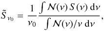 (1)where ν0 is the adopted nominal frequency of the filter. For the standard HFI and SPIRE pipelines, ν0 is chosen to be equal to 545 and 857 GHz, and to correspond to wavelengths of 350 and 500 μm, respectively. The parameter
  is the net spectral response in terms of absorbed power including the aperture efficiency, the filter spectral response, and for surface brightness the spectral dependence of the beam across the band (see, e.g., details in Griffin et al. 2013 and the SPIRE Handbook, Chap. 5). Its normalization is unimportant because the response is used only in ratios. Absolute calibration therefore requires precise knowledge of the instrument properties, particularly bandpasses and beams, and there are related uncertainties summarized here. See Appendix A for more details.
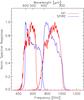 |
Fig. 1 Spectral response for the Planck/HFI 545 and 857 GHz filters (red) and the Herschel/SPIRE PLW and PMW filters (blue), respectively, each normalized relative to a maximum at unity. For SPIRE these include the spectral dependence of the beam across the band as is appropriate for extended emission (compare Figs. 5.16 to 5.5 in the SPIRE Handbook v2.5). No correction is needed for HFI. |
Recovering the true monochromatic brightness (or flux density), Sν0, from requires an instrument-dependent colour correction that depends on the shape of the SED, which varies over the sky. Because we are only interested in the relative calibration of the two instruments, these colour corrections are not needed explicitly. However, because of the different shapes of the spectral response functions for the pairs of bandpasses of the two instruments we are comparing (Fig. 1) and the different values of ν0, a bandpass correction dependent on the shape of the SED is needed for the cross-calibration analysis (see Sect. 4).
SPIRE fields selected for the SPIRE–HFI cross-calibration study.
The Planck/HFI calibration scheme for the 2015 PR2 data is described in Planck Collaboration VIII (2016). The 545 and 857 GHz channels were calibrated by comparing measurements of Uranus and Neptune flux densities with predictions based on models of their emissivities (the so-called Uranus ESA 2 and Neptune ESA 3 models produced by Moreno 2010 updating Moreno 1998). The statistical uncertainty of the measurements is 1.1% and 1.4% at 545 and 857 GHz, respectively, and the model predictions have an absolute uncertainty of 5%. Combining the statistical and systematic uncertainties linearly, the overall HFI absolute calibration uncertainty for PR2 data is 6.1% and 6.4% at 545 and 857 GHz, respectively.
The relative planet model uncertainty between these two HFI bands, however, is expected to be of order 2%. Combining the statistical uncertainties in quadrature (thus 1.8%) with this relative planet model uncertainty linearly, the relative uncertainty between the two bands would be about 3.8%.
As small bolometer to bolometer differences and variations over the sky have a negligible effect on our results (Appendix A.1), we used a Gaussian beam with a full width half maximum (FWHM) of  and
and  at 545 and 857 GHz, respectively (Planck Collaboration VII 2016).
The spectral responses shown in Fig. 1 are part of the Planck data release. We do not consider their uncertainties in this study; reported uncertainties on planet colour correction factors (Mars, Jupiter, Saturn, Uranus, Neptune) derived from these spectral responses are about 0.01% and 0.014% at 545 and 857 GHz, respectively (Planck Collaboration IX 2014).
Planck Collaboration XXX (in prep.) found that, with respect to the very accurate planet-independent calibration of the 100 and 143 GHz channels, the relative photometric calibration of the 545 GHz channel is + 2.3%±1.6% using the solar dipole and + 1.5%±1.8% using the first two cosmic microwave background (CMB) acoustic peaks (Appendix A.1). This suggests that the uncertainty of the planet-based absolute calibration of the 545 GHz channel is not as great as the value of 6.1% cited above, of which 5% arose from the absolute uncertainty of the planet model.
The photometric calibration of the Herschel/SPIRE instrument is described in detail in Bendo et al. (2013) and in the SPIRE Handbook. Calibration on the ESA 4 model of Neptune (Moreno 2012) introduces a 4% systematic uncertainty from model predictions. The statistical uncertainty on SPIRE photometry of the calibrators is about 1.5% (cf. Bendo et al. 2013) in the 350 μm (PMW) and 500 μm (PLW) bands. These two contributions add linearly to produce a 5.5% uncertainty in the point source calibration.
The pipeline processing used to produce the SPIRE maps needed in this paper made use of a conversion from point source flux density [Jy beam-1] to extended source surface brightness [ MJy sr-1] (Griffin et al. 2013), again for a reference spectrum νSref(ν) = constant. In the notation used in the SPIRE Handbook v2.5 the conversion factor may be written as KPtoE = (K4E/K4P)/Ωeff to highlight the inverse dependence on Ωeff, which is the so-called effective beam solid angle7 for that bandpass accounting for the frequency dependence of the beam and calculated for the reference spectrum. The ratio K4E/K4P of monochromatic conversion factors defined in the Handbook, also calculated for this reference spectrum, is close to unity. Following Table 5.2 of the SPIRE Handbook v2.5 as incorporated in the HIPE Version 12, the values of this ratio and Ωeff that we used are 1.0015 and 0.9993 and 822.58 arcsec2 and 1768.66 arcsec2, so that KPtoE is 51.799 and 24.039 MJy sr-1 Jy-1 for PMW and PLW, respectively. Underlying spectral responses of SPIRE for extended emission are shown in Fig. 1.
The uncertainty of KPtoE is dominated by the 4% uncertainty of the effective beam solid angles (Griffin et al. 2013). Adding this to the 5.5% uncertainty of the point source calibration, the total uncertainty of the extended source brightness calibration amounts to 9.5%. Ongoing efforts to improve the modelling of the radial beam profile are described in Appendix A.2 and the implication of any change is quantified in Sect. 7.
Although Neptune is the reference calibrator in common with both instruments (Uranus is also used for HFI), two different versions of the ESA model have been used. As described in Appendix A.3, the net effect of using the ESA4 model for the HFI calibration, combined with the absolute photometric calibration derived from Uranus model, would be an increase of HFI brightness of 0.31% and 0.16% at 545 and 857 GHz, respectively. Compared to the estimated uncertainties in cross-calibration relative gains found below in Sect. 5.2, this systematic uncertainty is not a major concern.
3. Field selection and map preparation
From the Herschel Science Archive (HSA)8 we selected 15 fields covering an appropriate range of average surface brightness and dynamics: two Science Demonstration Phase Hi-GAL fields at b = 0° (L59 centred at l = 59° and L30 at l = 30°), ten other fields in the Galactic plane from the Hi-GAL survey (Molinari et al. 2010), and three fields at higher latitude; these are Aquila (Könyves et al. 2010), Polaris (Miville-Deschênes et al. 2010), and Spider (in the North Celestial Pole Loop; e.g., Martin et al. 2015). Table 1 lists the field name, centre coordinates, size, and average surface brightness in the two Planck/HFI bands of interest.
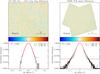 |
Fig. 2 Left: HFI 545 GHz noise map of the Polaris field obtained from the difference of the two independent half-ring maps of the same field (see text). The bottom panel shows the normalized histogram of brightnesses in the difference map (black) and a Gaussian fit to the distribution (red), with the mean μ, dispersion σ, and coefficient of determination R2 as an estimator of the “goodness of fit”9. Right: SPIRE PLW (500 μm) Polaris field noise map and histogram obtained from the difference between maps produced from scans in the nominal and orthogonal orientation, appropriately reweighted by the coverage map. The individual 3° × 3° and |

The SPIRE observations were carried out by mapping the field with a series of scans in one (the nominal) orientation and then a second time (with a different obsid) with a nearly orthogonal orientation (the cross-scan). Maps were made by processing simultaneously the data from scans in both the nominal and orthogonal orientations. For each field, we used the Level 0 SPIRE timelines products from the HSA. The observations are then processed with HIPE to produce PMW and PLW maps with pixel sizes 10′′ and 14′′, respectively. Destriping was applied using the Herschel/HIPE destriper module. A constant offset was also removed that is equal to the median flux level of the map, because SPIRE (like HFI) only measures relative fluxes, but this is of no consequence for the relative gain comparison.
The HFI maps of the same fields were produced as cutouts of the 545 and 857 GHz whole-sky HEALPix10 maps, corrected for zodiacal light, from the 2015 Planck data release (PR2; Planck Collaboration VIII 2016). We reprojected them on the SPIRE maps coordinates with a pixel size of 3′ × 3′.
Because the SPIRE beams are much smaller than those of HFI, we convolved the SPIRE maps with the HFI effective Gaussian beams (Sect. 2). We checked that the approximation of ignoring slight beam variations over the sky has a negligible impact on our analysis. Finally, we interpolated the convolved SPIRE maps to the HFI pixel grid.
3.1. Estimated noise maps
To estimate the high-frequency statistical noise for the HFI observations we took advantage of the redundancy of Planck observations during a stable pointing period (referred to as a ring; see Planck Collaboration VIII 2014). Among the products in the PR2 release there are two independent HFI maps produced by splitting each ring into two equal duration parts, the so-called half-ring maps (Planck Collaboration VIII 2016, Appendix A.1). The noise is assessed using the difference of cutouts from the two half-ring maps, following the method described in Miville-Deschênes et al. (2002) and Miville-Deschênes & Lagache (2005) in which the noise is assumed to be stationary. The histogram of the brightnesses in these difference maps is very well described by a Gaussian in all the fields (see, e.g., the fit in Fig. 2, lower left, for the HFI Polaris field). The final estimated noise map (e.g., Fig. 2, upper left) is weighted using the coverage. We note that this estimate is consistent with realizations based on the PR2 variance map (Planck Collaboration VIII 2016).
The procedure for SPIRE was similar. We made separate maps from data for scans in each of the two orthogonal orientations (the two separate obsids) separately, creating a difference map that was then weighted by the coverage. In some SPIRE fields the histograms for the difference maps showed distributions that are slightly broader than the central Gaussian core with low amplitude tails at high and low values of brightness difference. These are mostly due to 1 /f noise (see also Sect. 6.1 below) that is not perfectly removed when a map is produced from data in only a single scan orientation, as opposed to both (this is the fundamental reason for this observational strategy). Varying spatial coverage between the orthogonal sets of observations, which is especially apparent along the map edges, also contributes to broadening the histogram. However these effects, which are already small at the SPIRE angular resolution, become completely negligible when the fields are brought to the HFI angular resolution. Similarly, the values shown here for the SPIRE difference maps are not directly comparable to the noise estimates discussed in Sect. 5.1 because the HFI 545 and 857 GHz beams encompass roughly 450 and 870 pixels in the corresponding SPIRE map, respectively. At the same resolution and pixelization the distribution of SPIRE noise has a much smaller variance than is found for the noise in the HFI map.
The SPIRE Polaris field (Fig. 2, right, and Fig. 8 below) is a special case, since it is the result of mapping two overlapping subfields11 (hence two pairs obsids), and the effect of weighting by the coverage is clearly seen in the estimated noise map.
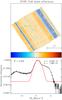 |
Fig. 3 Same as Fig. 2 but for a SPIRE difference map dominated by systematic effects (Hi-GAL field 37_0, |

Finally, we note that several additional fields were initially part of the analysis but were discarded because they displayed strong residual effects. An example of such a field is shown in Fig. 3. As a result of these residual systematic effects, adding such fields would not improve the accuracy of the joint estimate of the cross-calibration relative gain. Similarly, lower brightness fields are not useful because the instrumental noise limits the accuracy of the comparison.
4. Bandpass corrections
To compare flux density or brightness measurements from two different instruments, it is necessary to apply a correction that takes the differences in their respective net spectral responses into account. This bandpass correction should not to be confused with the standard colour correction that, for a given bandpass, converts the brightness obtained at the nominal frequency from a given SED to that from another SED. A bandpass correction converts, for a given SED, the brightness obtained at the nominal frequency from a given bandpass to the brightness that would be obtained from another bandpass. Because the SED varies both within a given field and from field to field, bandpass corrections are essential in preparing the data for assessment of the cross-calibration relative gain; a corollary is that there is no unique bandpass conversion factor between the uncorrected HFI and SPIRE data.
Although the two pairs of HFI and SPIRE bandpasses are similar, they are nevertheless sufficiently different that bandpass corrections are required, especially in the case of the 545 GHz and 500 μm bandpasses which overlap by only about two-thirds (see Fig. 1). Only after the bandpass correction has been applied can one compare the two independent brightness measurements to investigate whether the absolute calibrations are consistent within their uncertainties. Technically, this comparison gives the desired measurement of the cross-calibration relative gain, which is expected to be independent of the SED and field on the sky.
4.1. Definition
As described in Sect. 2, Herschel/SPIRE and Planck/HFI each provides maps of monochromatic surface brightnesses , at their individual reference frequency ν0, assuming a reference spectrum νSref(ν) = constant (see Eq. (1)). We need a bandpass correction KHFI− > SPIRE to convert the observed brightness from HFI (at ν0H) to that which would be observed in the paired SPIRE bandpass (at ν0S), so that the bandpass-corrected HFI map can be compared to the SPIRE map. Thus 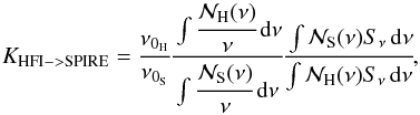 (2)where
  and
and  are the net spectral responses for extended emission for HFI and SPIRE, respectively (as shown in Fig. 1).
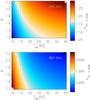 |
Fig. 4 Correction factors from measurements with HFI to what would be observed by SPIRE, KHFI− > SPIRE (Eq. (2)), for MBB spectra (Eq. (3)) with a range of temperatures, TBB, and emissivity indices, β, at the two HFI frequencies. We decreased the resolution along the temperature axis by a factor of 10 compared to the tabulated values to a step of 1 K. The anti-correlation between TBB and β can produce the same MBB SED shape across the bandpass and, hence, the same correction. |
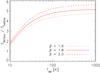 |
Fig. 5 Planck/HFI 857 to 545 GHz brightness ratio versus MBB spectrum temperature, TBB, for three different values of the emissivity index (β = 1.6, 1.8, and 2.0). For our application, dust temperatures would be in the low end of the range, allowing some discrimination of TBB. |
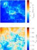 |
Fig. 6 Top: HFI 545 GHz spanning the Polaris field. Bottom: KHFI− > SPIRE bandpass correction, K545 at 545 GHz (Eq. (4)), for the same field. |
4.2. Evaluating the bandpass correction
Equation (2)shows that KHFI− > SPIRE depends on the shape of the source SED, Sν. In rare cases Sν is well known beforehand (e.g., for a calibration source) but in general its shape has to be estimated (or assumed).
A simple and robust model of the SED of thermal emission by Galactic dust in the submillimetre range is a modified blackbody (MBB) spectrum with a temperature, TBB, and emissivity index, β, in the form  (3)Typical TBB and β values for diffuse dust emission, which is the dominant component in the selected maps, range from 10 to 40 K and 1.4 to 2.5, respectively (e.g. Planck Collaboration XI 2014; Paradis et al. 2010).
We used Eqs. (2)and (3)to produce tables of the KHFI− > SPIRE bandpass-correction factors  (4)for a range of TBB from 10 to 40 K with a step of 0.1 K, and a range of β from 1.2 to 2.2 with a step of 0.05. These are shown in Fig. 4.
Several approaches can be used to estimate TBB and β from the data, one of which is to fix the emissivity index at an appropriate value deduced from previous studies and deduce the temperature from the measured ratio Planck/HFI 857 to 545 GHz brightness ratio (Fig. 5). This ratio could be obtained from standard linear regression between the two entire maps, but this would not take local temperature variations into account, and these variations can be important. Alternatively, the temperature can be deduced from the brightness ratio at each pixel. This is implemented in the HIPE pipeline developed to determine SPIRE maps offsets, with 8′-resolution Planck maps.
We implemented a second option, exploiting full-sky maps of TBB and β produced from multi-frequency data as part of the Planck products (Planck Collaboration XI 2014; Planck Collaboration 2013). Neither TBB and β are individually important as long as, together in Eq. (3), they describe the slope of the SED that are fit in the data. Thus at every HFI pixel we can readily estimate the bandpass correction by interpolation in the above tables of K, producing bandpass-correction maps. An example is shown in Fig. 6 for the Polaris field at 545 GHz. We note that the bandpass corrections are different from pixel to pixel, with a range that is large compared to the uncertainty that we find for the cross-calibration relative gain below. Thus accurately computing and applying bandpass corrections is essential.
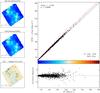 |
Fig. 7 Correlation and pixel-to-pixel comparison between HFI and SPIRE observations of the Hi-GAL L59 field at 545 GHz. Top left: HFI and SPIRE maps of the L59 field. Top right: SPIRE–HFI pixel-to-pixel correlation. The linear fit from the unweighted “X on Y” regression is plotted in red, with the 1-to-1 line in black for reference. The offset removed from the SPIRE map during the map-making has been obtained from the fit and added back. Bottom right: horizontal residuals from the fit, as a function of brightness. Bottom left: map of the horizontal residuals, with a colour range that is ten times finer (centred on 0), to enhance the details. |
5. Pixel-to-pixel comparison
After bandpass correction with KHFI− > SPIRE an observation of a field with HFI should yield brightnesses equal to those measured with SPIRE (but the latter is missing an offset). This appears to be the case, as illustrated in Fig. 7. Any difference in slope compared to unity should be consistent with (or lower than) the combination of reported absolute calibration errors.
5.1. Degree of correlation
The Pearson correlation coefficient between the pixel brightnesses in the two maps ( in map i, in MJy sr-1) is the ratio of their covariance to the product of their standard deviations σi (not to be confused with statistical uncertainties), i.e.
 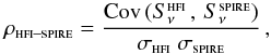 (5)which is unaffected by potential difference between the two calibrations. Therefore, we use the Pearson correlation coefficient to assess the degree of linear correlation between the SPIRE and HFI surface brightnesses in a map. In the presence of noisy variables, the computed correlation coefficient,
  , always underestimates the true value (see Sect. 5.3).
Estimated correlation coefficients for each field at the two frequency bands are reported in Table 2. They average to 0.9986 (± 0.08%) and 0.9985 (± 0.07%) at 545 and 857 GHz, respectively. This high degree of linear correlation between the SPIRE and HFI signals, although expected, confirms that the SPIRE/HFI relative gain does not depend on brightness and is a useful validation that a simple linear fit procedure can be used to derive the cross-calibration relative gain and the SPIRE map offsets (Sect. 5.2).
5.2. Relative gain measurements
We used scatter plots to estimate the relative gain (GScat) between the two instruments. Following the hypothesis of linearity as demonstrated in Sect. 5.1, the relative gain is the slope of the correlation, independent of the zero levels. However, the same procedure can be used to find and restore the offset that has been removed from the SPIRE map during the map-making. Thus, the relationship is  (6)Because the noise in the HFI map is considerably larger than in the convolved SPIRE map (Sect. 3.1), in practice we carried out the unweighted fit to the data in the sense of a regression of “X on Y” rather than “Y on X” and then inverted the slope to correspond to GScat as written in Eq. (6).
An example of the SPIRE–HFI scatter plot and computed linear fit is shown in Fig. 7 for the L59 field of the Hi-GAL survey. This analysis has been carried out for the 15 selected fields for the two frequency bands. Results for the relative gains, the slopes of the linear fits, are given in Table 2. The average and standard deviation of the estimated values of GScat is 1.047 (± 0.0069) and 1.003 (± 0.0080) at 545 and 857 GHz, respectively.
Estimates of the relative gains, GScat, and Pearson correlation coefficients,  , at 545 and 857 GHz.
5.3. Comparison of estimates of the uncertainty in the HFI maps
Considering that the uncertainties in the convolved SPIRE maps are very small in comparison to the uncertainties in the HFI maps, we can attribute the dispersion about the regression line to the HFI uncertainties alone. We can estimate the 1σ uncertainty,  , from the dispersion of the residuals in the horizontal direction:
  . For the example L59 field, these residuals are shown in the lower panels of Fig. 7.
Under the assumption of Gaussianity of the noise in our maps, which is reasonable here as shown in Sect. 3.1, the Pearson correlation coefficient allows us to make an alternative estimate, a posteriori, of the noise in the HFI maps. Assuming that the measured signal can be written as Smeas = Strue + Snoise, which is a reasonable assumption, the computed correlation coefficient reads ![Mathematical equation: \begin{equation} \hat{\rho}_\text{\sc hfi--spire} = \left[\left(1 + \frac{u_{\text{\sc hfi}}^2}{\sigma_{\text{\sc hfi}}^2} \right) \ \left(1 + \frac{u_{\text{\sc spire}}^2}{\sigma_{\text{\sc spire}}^2} \right) \right]^{-1/2} \ \rho_\text{\sc hfi--spire} , \label{eqn:rho_tilde} \end{equation}](/articles/aa/full_html/2016/04/aa27313-15/aa27313-15-eq105.png) (7)where ui are 1σ uncertainties of the brightnesses characterizing Snoise. In our selected fields, the signal variance
(7)where ui are 1σ uncertainties of the brightnesses characterizing Snoise. In our selected fields, the signal variance  is much higher than that of the uncertainty, i.e.
  in both SPIRE and HFI maps. Furthermore, as discussed above,
  . Thus Eq. (7) simplifies to
 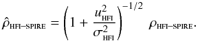 (8)Because
  , we can use the variance of the measured HFI brightness as a first order estimate of
  (the variance of the true, noiseless signal). Furthermore, we can assume that ρhfi–spire = 1 on the RHS. Using the computed Pearson correlation coefficients
  in Table 2 on the LHS, we solve Eq. (8)for uHFI, designating this a posteriori estimate as
  .
.
In the last two columns (for the two frequency bands) of Table 2, we tabulate the percentage difference of these two estimates for each field:  . As expected, we find these to be in very good agreement (better than 0.4%). The overall consistency further demonstrates that the gain does not depend on brightness and is consistent with the HFI brightness uncertainties dominating over those of SPIRE.
5.4. Contributions to the error budget for GScat
The relative gains in Table 2 show that at 857 GHz the SPIRE and HFI photometric calibrations agree to within 1%. However, at 545 GHz there is a 4.7% discrepancy that is statistically significant (6.8σ). Each instrument has absolute calibration errors that were discussed in Sect. 2. As we showed in Appendix A.3, the Neptune models used for calibration of the two instruments are very close and can only explain at most a 0.31% departure from unity. Furthermore, the statistical measurement error from each instrument combined quadratically amount to an uncertainty of 1.86% and 2.06% in the relative gain at 545 and 857 GHz. However, the SPIRE effective beam solid angle has an uncertainty of 4% (Griffin et al. 2013), acting as a systematic effect on the SPIRE photometric calibration and thus on the gain estimates as well. This dominates the Planck/Herschel cross-calibration error budget presented here and could account for the observed 4.7% discrepancy at 545 GHz; the potential revision of the value of the solid angle discussed in Appendix A.2 would reduce the discrepancy to 2.7%.
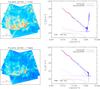 |
Fig. 8 Left: SPIRE PLW and PMW maps of the Polaris field. The black square outlines the region of the map that is used to compute the power spectra shown on the right. Right: power spectra of SPIRE map (blue) and bandpass-corrected HFI (red) map for PLW (top) and PMW (bottom) in the Polaris field. The solid lines are the dust power spectra obtained from the image power spectra (dashed line), from which the noise spectra (dotted line) are subtracted followed by division by the effective beam power spectra (dash dotted line; arbitrarily shifted on the y-axis). |
6. Cross calibration with power spectrum measurements
Power spectra offer a means of probing the spatial structure of diffuse emission. In our context, we can use power spectra to search for any scale dependence of the relative gain. This scale dependence is not expected, but can be introduced artificially by the data processing (any filtering process and the map-making). It is therefore of particular interest to check the level of agreement between power spectra of bandpass-corrected maps produced by Planck/HFI and those from Herschel/SPIRE.
However, the HFI and SPIRE spatial resolutions differ greatly and that of HFI limits the largest spatial frequency (lowest spatial scale) for comparison to about k = 0.3 arcmin-1. As a result of map pixelization effects, we actually limit our power spectrum comparison to k< 0.1 arcmin-1. Furthermore, the SPIRE fields are limited in sky coverage, which limits the smallest spatial frequency to about k = 0.007 arcmin-1 (proportionately lower for the three larger fields). At those scales, variations in the power spectra are dominated by cosmic variance but because cosmic variance is the same for the two maps it need not be considered in the comparison. This is not a large range in scale but thanks to the number of fields the power spectrum comparison still allows us to check for any systematic scale dependence of the gain.
6.1. Implementation
We implement the estimation of the power spectrum based on the methodology presented in Miville-Deschênes et al. (2002) via the IDL FFT routine. In overview, the power spectrum of an image Sx,y whose Fourier transform is  is computed from the map of the amplitude Akx,ky defined by
  (9)The power spectrum P(k) dk is an angular average of Akx,ky between k and k + dk, where
  .
.
To compare the power spectra of the dust signal we need to take the noise contamination and the effect of beam convolution into account. Formally,  (10)where bn(k) is the noise power spectrum and B(k) the beam power spectrum. The noise power spectrum is computed from the estimated noise maps produced from redundant observations, as described in Sect. 3.1. As mentioned, there is a 1 /f noise component in the SPIRE estimate, which is clearly visible in the noise power spectra in Fig. 8. This component is not in the SPIRE power spectra computed on the total map, but because this component is about 20−50 times smaller than signal power spectrum at low k it does not impact our analysis.
In Fig. 8 we show how the deconvolved SPIRE power spectrum at full resolution compares to that from HFI. This comparison is qualitatively interesting; as in the pixel-to-pixel comparison, we see a very good agreement across the range of spatial frequencies common to both instruments. Furthermore, the same power-law exponent appears to apply at the higher spatial frequencies accessible only to SPIRE, which is consistent with the study by Miville-Deschênes et al. (2010).
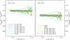 |
Fig. 9 Relative gain, from the square root of the SPIRE-to-HFI power spectrum ratio, for each field at 545 GHz (left) and 857 GHz (right). The mean gain GPSD from the power spectrum analysis (solid line) is in close agreement with the mean gain GScat from pixel-to-pixel analysis (dotted line), which is well within the 1σ dispersion of the latter (shaded in grey). |
6.2. Relative gain from power spectra
To compare SPIRE and HFI photometric calibrations quantitatively, we compute P(k) on the bandpass-corrected HFI maps and on the SPIRE maps brought to the HFI resolution. This mitigates against errors due to beam accuracy and differences in pixel window functions.
The HIPE pipeline does not optimize the orientation of the final image to be used in the power spectrum analysis and so our maps feature zero coverage on the corners. Rather than rotating the WCS, which would lead to significant distortion at small scales in the power spectrum, or cropping our data to small full-coverage insets (which was sufficient for the purposes of Fig. 8), which would reduce the range of overlapping scales, we zero-averaged our images and padded them with zeros. This masking operation in the image, which corresponds to a convolution of the true power spectrum in Fourier space, is carried out on both SPIRE and HFI maps, and so does not affect the power spectrum ratio and thus the relative gain determination.
The relative gain is the square root of ratio of the two power spectra, i.e.  (11)The relative gain is shown in Fig. 9 for each field, where it is seen that there is good agreement from field to field. The average (and rms) GPSD over the spatial scales analysed is 1.043 (± 0.012) and 0.995 (± 0.015) at 545 and 857 GHz, respectively. These estimates are in very good agreement (better than 1σ) with the pixel-to-pixel average gains GScat in Table 2.
To search for any variation with spatial scale, we calculated the average GPSD(k) in five bins of k across the range 0.007−0.1 arcmin-1. For both frequencies we found the relative gains GPSD(k) to be stable with scale with rms variations lower than about 1.5%.
7. Conclusion
We performed a detailed comparison of the Herschel/SPIRE and Planck/HFI absolute photometric calibration. We produced SPIRE maps for 15 fields that contain bright diffuse emission using publicly released Herschel data. These maps were corrected for bandpass differences, reprocessed to match the HFI angular resolution and pixelization, and then compared to their Planck counterparts from publicly released data. The comparison was carried out using two methods: a pixel-to-pixel comparison and a power spectrum analysis. We discarded several fields that were originally in the study to limit systematic effects arising from significant SPIRE processing residuals and to maintain a high signal-to-noise ratio in the maps and a high accuracy in the comparison.
The pixel-to-pixel comparison revealed the expected very high degree of linearity between the two datasets, and allowed for a robust estimate of the relative gain between the two instruments in each of the overlapping bands. The power spectrum analysis provided gain estimates with similar values and comparable statistical uncertainties. The good agreement of the relative calibration measured on distinct fields shows robustness to a number of potential systematic errors in either instrument, including nonlinear response, uncorrected time variability in the gain, and variation of the effective beam.
We found that the estimated relative gains are well inside the absolute photometric uncertainties quoted for the two instruments of about 6.4% and 9.5% for HFI and SPIRE, respectively. However, because both instruments use the same planetary calibrator, that contribution to the relative uncertainty can be reduced to the very small difference between the ESA 3 and ESA 4 models of Neptune. Then the deviations are comparable to the remaining uncertainty values of 1.4% and 5.5% for HFI and SPIRE. The difference in the ESA 3 and ESA 4 Neptune models used in the HFI and SPIRE calibrations, respectively, decreases the two relative gain estimates by only a very small fraction (0.31% at 545 GHz and 0.16% at 857 GHz).
At 545 GHz the departure of the relative gain from unity is statistically significant, which raises the question of whether a systematic calibration correction should be applied prior to any comparative analysis between HFI maps at 545 GHz and SPIRE maps at 500 μm. However, this departure could be accounted for by the 4% systematic uncertainty of the SPIRE beam solid angle. Because this dominates the error budget of the SPIRE–HFI cross calibration, we provide here the SPIRE/HFI relative gains with their explicit dependence on the SPIRE unit conversion factor KPtoE as follows:  (12)and
  (13)at 545 and 857 GHz (or PLW and PMW), respectively, where the normalizations of KPtoE are our adopted values in MJy sr-1 Jy-1. These formulae would be useful for any future analysis that might make use of an updated version of the SPIRE KPtoE (see e.g. Appendix A.2).
We used two methods of comparison, both based on extended emission, but did not make a comparison based on point sources. There are SPIRE counterparts for many extragalactic sources of the Planck point source catalogue (e.g., in the fields of H-ATLAS; Eales et al. 2010), but confusion noise at the Planck/HFI channels induces uncertainties in point source photometry that are too large for an accurate estimate of the cross calibration of the two instruments, especially compared to the level of precision that can be achieved with maps of diffuse emission.
Planck (http://www.esa.int/Planck) is a project of the European Space Agency (ESA) with instruments provided by two scientific consortia funded by ESA member states and led by Principal Investigators from France and Italy, telescope reflectors provided through a collaboration between ESA and a scientific consortium led and funded by Denmark, and additional contributions from NASA (USA).
Herschel (http://www.esa.int/Herschel) is an ESA space observatory with science instruments provided by European-led Principal Investigator consortia and with important participation from NASA.
The SPIRE Handbook is available at http://herschel.esac.esa.int/Docs/SPIRE/spire_handbook{.}pdf.
For a preview, see http://herschel.esac.esa.int/TheUniverseExploredByHerschel/posters/B23_SchulzB{.}pdf
The spectral energy distribution (the SED) is often denoted Iν in the case of surface brightness and Fν in the case of point source flux densities. In this paper we will use Sν for both, the distinction being clear from the context. The pipeline product that we denote is called Spip in the SPIRE Handbook.
This solid angle results from integration of the beam over 4π steradians, as distinct from the main beam solid angle for the main lobe, and hence corresponds to what elsewhere is called the antenna beam solid angle (see, e.g., http://ipnpr.jpl.nasa.gov/progress_report/42-64/64T{.}PDF).
The coefficient of determination provides a measure of the fraction of variance of the data explained by the model.
The structural and statistical properties of the subfield extending to the upper left were studied by Miville-Deschênes et al. (2010) using a power spectrum analysis.
Acknowledgments
We thank Jean-Loup Puget for insightful discussions. B.B. is particularly thankful to Marc-Antoine Miville-Deschênes for providing us pre-release access to the Spider SPIRE data. B.B. acknowledges the support of a CNES post-doctoral research grant. We thank the referee, Bernard Lazareff, for helpful comments that have led to improvements in the manuscript. The Planck Collaboration acknowledges the support of: ESA; CNES, and CNRS/INSU-IN2P3-INP (France); ASI, CNR, and INAF (Italy); NASA and DoE (USA); STFC and UKSA (UK); CSIC, MINECO, JA and RES (Spain); Tekes, AoF, and CSC (Finland); DLR and MPG (Germany); CSA (Canada); DTU Space (Denmark); SER/SSO (Switzerland); RCN (Norway); SFI (Ireland); FCT/MCTES (Portugal); ERC and PRACE (EU). A description of the Planck Collaboration and a list of its members, indicating which technical or scientific activities they have been involved in, can be found at http://www.cosmos.esa.int/web/planck/planck-collaboration.
References
- Bendo, G. J., Griffin, M. J., Bock, J. J., et al. 2013, MNRAS, 433, 3062 [NASA ADS] [CrossRef] [Google Scholar]
- Eales, S., Dunne, L., Clements, D., et al. 2010, PASP, 122, 499 [NASA ADS] [CrossRef] [Google Scholar]
- Górski, K. M., Hivon, E., Banday, A. J., et al. 2005, ApJ, 622, 759 [NASA ADS] [CrossRef] [Google Scholar]
- Griffin, M. J., Abergel, A., Abreu, A., et al. 2010, A&A, 518, L3 [Google Scholar]
- Griffin, M. J., North, C. E., Schulz, B., et al. 2013, MNRAS, 434, 992 [NASA ADS] [CrossRef] [Google Scholar]
- Juvela, M., Ristorcelli, I., Pelkonen, V.-M., et al. 2011, A&A, 527, A111 [NASA ADS] [CrossRef] [EDP Sciences] [Google Scholar]
- Könyves, V., André, P., Men’shchikov, A., et al. 2010, A&A, 518, L106 [NASA ADS] [CrossRef] [EDP Sciences] [Google Scholar]
- Lindal, G. F. 1992, AJ, 103, 967 [NASA ADS] [CrossRef] [Google Scholar]
- Martin, P. G., Blagrave, K. P. M., Lockman, F. J., et al. 2015, ApJ, 809, 153 [NASA ADS] [CrossRef] [Google Scholar]
- Miville-Deschênes, M.-A., & Lagache, G. 2005, ApJS, 157, 302 [NASA ADS] [CrossRef] [Google Scholar]
- Miville-Deschênes, M.-A., Lagache, G., & Puget, J.-L. 2002, A&A, 393, 749 [NASA ADS] [CrossRef] [EDP Sciences] [Google Scholar]
- Miville-Deschênes, M.-A., Martin, P. G., Abergel, A., et al. 2010, A&A, 518, L104 [NASA ADS] [CrossRef] [EDP Sciences] [Google Scholar]
- Molinari, S., Swinyard, B., Bally, J., et al. 2010, A&A, 518, L100 [NASA ADS] [CrossRef] [EDP Sciences] [Google Scholar]
- Moreno, R. 1998, Ph.D. Thesis, Université Paris 6, France [Google Scholar]
- Moreno, R. 2010, Technical Report, Neptune and Uranus planetary brightness temperature tabulation, ftp://ftp.sciops.esa.int/pub/hsc-calibration/PlanetaryModels/ESA2, and 3 (ESA) [Google Scholar]
- Moreno, R. 2012, Technical Report, Neptune and Uranus planetary brightness temperature tabulation, ftp://ftp.sciops.esa.int/pub/hsc-calibration/PlanetaryModels/ESA4 (ESA) [Google Scholar]
- Paradis, D., Veneziani, M., Noriega-Crespo, A., et al. 2010, A&A, 520, L8 [NASA ADS] [CrossRef] [EDP Sciences] [Google Scholar]
- Pilbratt, G. L., Riedinger, J. R., Passvogel, T., et al. 2010, A&A, 518, L1 [CrossRef] [EDP Sciences] [Google Scholar]
- Planck Collaboration XVIII. 2011, A&A, 536, A18 [NASA ADS] [CrossRef] [EDP Sciences] [Google Scholar]
- Planck Collaboration XXII. 2011, A&A, 536, A22 [NASA ADS] [CrossRef] [EDP Sciences] [Google Scholar]
- Planck Collaboration 2013, The Explanatory Supplement to the Planck 2013 results, http://wiki.cosmos.esa.int/planckpla/index.php/CMB_and_astrophysical_co mponent_maps#Thermal_dust_emission (ESA) [Google Scholar]
- Planck Collaboration VI. 2014, A&A, 571, A6 [NASA ADS] [CrossRef] [EDP Sciences] [Google Scholar]
- Planck Collaboration VIII. 2014, A&A, 571, A8 [NASA ADS] [CrossRef] [EDP Sciences] [Google Scholar]
- Planck Collaboration IX. 2014, A&A, 571, A9 [NASA ADS] [CrossRef] [EDP Sciences] [Google Scholar]
- Planck Collaboration XI. 2014, A&A, 571, A11 [NASA ADS] [CrossRef] [EDP Sciences] [Google Scholar]
- Planck Collaboration VII. 2016, A&A, in press, DOI: 10.1051/0004-6361/201525844 [Google Scholar]
- Planck Collaboration VIII. 2016, A&A, in press, DOI: 10.1051/0004-6361/201525820 [Google Scholar]
- Viero, M. P., Wang, L., Zemcov, M., et al. 2013, ApJ, 772, 77 [NASA ADS] [CrossRef] [Google Scholar]
Appendix A: Notes regarding absolute photometric calibration
The absolute calibration of the two instruments is described in Sect. 2. Some supplementary details are provided here.
Appendix A.1: Planck/HFI
HFI is a scanning instrument and its effective beams relevant to the frequency maps are the convolution of (i) the optical response of the telescope and feeds; (ii) the processing of the time-ordered data and deconvolution of the time response; and (iii) the merging of several surveys to produce frequency maps. While accurate effective beams can be recovered at each sky position, this is a time-consuming process. However, the rms variations of the effective beam solid angle across the sky are 0.79% and 0.49% at 545 and 857 GHz, respectively (see Table 3 in Planck Collaboration VII 2016), which are negligible with respect to the calibration uncertainty, and so ignoring the spatial variation has a negligible effect for our study of diffuse emission calibration. Therefore, for convenience of implementation in our processing pipeline we decided to use an effective Gaussian beam instead, as cited in Sect. 2.
Accurate knowledge of the spectral response is essential for comparing surface brightness obtained through different filters or for computing colour corrections. Spectral responses for Planck/HFI were measured pre-flight for each detector and checked with ground and in-flight data (see Planck Collaboration IX 2014). As noted in Sect. 2, these are known with sufficient accuracy not to impact the results in this paper.
The photometric calibration for the Planck/HFI channels which are CMB dominated (100, 143, and 217 GHz) or have a strong enough CMB signal (353 GHz) is achieved through observations of the dipole arising from the orbital motion of the Planck spacecraft around the Sun (the orbital dipole). The calibration accuracy is very high, 0.09% and 0.07% at 100 and 143 GHz, respectively (Planck Collaboration VIII 2016).
The 545 GHz channel and even more so the 857 GHz channel cannot be calibrated on the orbital dipole, which is too weak with respect to Galactic dust emission, and so, as described above, these were calibrated using Uranus and Neptune. Nevertheless, given the high absolute calibration accuracy at 100 and 143 GHz, the relative photometric calibration of the 545 GHz channel with respect to those two channels can be used to assess the accuracy of the 545 GHz planet-based absolute calibration.
Planck Collaboration XXX (in prep.) have used the dipole generated by the solar system motion with respect to the CMB (the solar dipole) and the first two acoustic peaks of the CMB fluctuations to measure the relative calibration of all Planck/HFI channels, except 857 GHz, adopting the average of 100 and 143 GHz as reference. As summarized in Sect. 2, it was found that the planet-calibrated data at 545 GHz has a relative calibration of + 2.3%±1.6% using the solar dipole and + 1.5%±1.8% using the first two CMB peaks. This is remarkable and suggests that the uncertainty of the planet-based absolute calibration of the 545 GHz channel is not as great as the value of 6.1% cited in Sect. 2. Recall that 5% arose from the estimated absolute uncertainty of the planet model predictions, (Planck Collaboration VIII 2016) which relates mostly to uncertainties on the thermal profiles from Lindal (1992). Even if the uncertainty were that large, the relative planet model uncertainty between these two HFI bands is expected to be of order 2%.
The previous Planck 2013 data release (PR1) also relied on the Neptune and Uranus models for absolute calibration. Improvements in the data processing and calibration procedure shifted the final absolute calibration of frequency maps by −1.8% and −3.3% at 545 and 857 GHz, respectively (the 2015 PR2 maps are fainter).
Appendix A.2: Herschel/SPIRE
The uncertainty of the conversion factor KPtoE (Sect. 2) is dominated by the 4% uncertainty of the effective beam solid angles, Ωeff. We adopted values from Griffin et al. (2013) (HIPE Version 12).
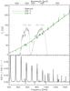 |
Fig. A.1 Top: comparison of the ESA 3 (dashed black) and ESA 4 (green) Neptune models. Corresponding flux densities in the 545 and 857 GHz HFI bands are shown as triangles (ESA 3) and squares (ESA 4). Bottom: relative difference of the two model spectra and the flux densities. |
Ongoing efforts to improve the modelling of the radial beam profile have revised the values of Ωeff to 1804.3 ± 13 arcsec2 (±0.7%) and 831.4 ± 3.8 arcsec2 (±0.5%) for PLW and PMW, respectively. These amount to increases of just 2.0% and 1.1%; furthermore, we note that the stated uncertainties in Ωeff are now considerably less than the 4% cited above. Adopting the revised values of Ωeff would decrease the above conversion factors KPtoE and thus decrease the brightness of the SPIRE maps and the SPIRE/HFI relative gains estimated in this paper (Eqs. (12) and (13)).
Although these values have been incorporated in HIPE Version 1412, nevertheless, until such time as revised beam solid angles are adopted officially in the SPIRE Handbook, and to facilitate tracking of dependencies and changes, we felt it prudent to frame our results in terms of the cited values from the version of HIPE that we used (Version 12), consistent with the values from the latest SPIRE Handbook, v2.5.
Appendix A.3: Neptune models
As seen in Fig. A.1, the main differences between the ESA 3 model of Nepture used for the HFI calibration, and the ESA 4 model of Nepture used for the SPIRE calibration rest in an updated treatment of the CO absorption features and HCN emission lines. Several of these features fall within the HFI and SPIRE bands and so affect estimates of the cross-calibration
factor as a systematic error. We computed HFI equivalent Neptune flux densities for both models and find that, if calibrated on ESA 4 rather than ESA 3, the HFI absolute calibration factors on Neptune would increase by 0.63% and 0.31% at 545 and 857 GHz, respectively (see bottom panel of Fig. A.1). Combined with the absolute photometric calibration of HFI derived from Uranus model, these drop down to an increase of 0.31% and 0.16% at 545 and 857 GHz, respectively. We note that an increase of the HFI calibration factors translates into an increase of HFI brightness and thus a decrease of the SPIRE / HFI relative gains that we estimate in this paper (Eqs. (12) and (13)).
All Tables
Estimates of the relative gains, GScat, and Pearson correlation coefficients, , at 545 and 857 GHz.
All Figures
|
Fig. 1 Spectral response for the Planck/HFI 545 and 857 GHz filters (red) and the Herschel/SPIRE PLW and PMW filters (blue), respectively, each normalized relative to a maximum at unity. For SPIRE these include the spectral dependence of the beam across the band as is appropriate for extended emission (compare Figs. 5.16 to 5.5 in the SPIRE Handbook v2.5). No correction is needed for HFI. |
| In the text | |
|
Fig. 2 Left: HFI 545 GHz noise map of the Polaris field obtained from the difference of the two independent half-ring maps of the same field (see text). The bottom panel shows the normalized histogram of brightnesses in the difference map (black) and a Gaussian fit to the distribution (red), with the mean μ, dispersion σ, and coefficient of determination R2 as an estimator of the “goodness of fit”9. Right: SPIRE PLW (500 μm) Polaris field noise map and histogram obtained from the difference between maps produced from scans in the nominal and orthogonal orientation, appropriately reweighted by the coverage map. The individual 3° × 3° and |
| In the text | |
|
Fig. 3 Same as Fig. 2 but for a SPIRE difference map dominated by systematic effects (Hi-GAL field 37_0, |
| In the text | |
|
Fig. 4 Correction factors from measurements with HFI to what would be observed by SPIRE, KHFI− > SPIRE (Eq. (2)), for MBB spectra (Eq. (3)) with a range of temperatures, TBB, and emissivity indices, β, at the two HFI frequencies. We decreased the resolution along the temperature axis by a factor of 10 compared to the tabulated values to a step of 1 K. The anti-correlation between TBB and β can produce the same MBB SED shape across the bandpass and, hence, the same correction. |
| In the text | |
|
Fig. 5 Planck/HFI 857 to 545 GHz brightness ratio versus MBB spectrum temperature, TBB, for three different values of the emissivity index (β = 1.6, 1.8, and 2.0). For our application, dust temperatures would be in the low end of the range, allowing some discrimination of TBB. |
| In the text | |
|
Fig. 6 Top: HFI 545 GHz spanning the Polaris field. Bottom: KHFI− > SPIRE bandpass correction, K545 at 545 GHz (Eq. (4)), for the same field. |
| In the text | |
|
Fig. 7 Correlation and pixel-to-pixel comparison between HFI and SPIRE observations of the Hi-GAL L59 field at 545 GHz. Top left: HFI and SPIRE maps of the L59 field. Top right: SPIRE–HFI pixel-to-pixel correlation. The linear fit from the unweighted “X on Y” regression is plotted in red, with the 1-to-1 line in black for reference. The offset removed from the SPIRE map during the map-making has been obtained from the fit and added back. Bottom right: horizontal residuals from the fit, as a function of brightness. Bottom left: map of the horizontal residuals, with a colour range that is ten times finer (centred on 0), to enhance the details. |
| In the text | |
|
Fig. 8 Left: SPIRE PLW and PMW maps of the Polaris field. The black square outlines the region of the map that is used to compute the power spectra shown on the right. Right: power spectra of SPIRE map (blue) and bandpass-corrected HFI (red) map for PLW (top) and PMW (bottom) in the Polaris field. The solid lines are the dust power spectra obtained from the image power spectra (dashed line), from which the noise spectra (dotted line) are subtracted followed by division by the effective beam power spectra (dash dotted line; arbitrarily shifted on the y-axis). |
| In the text | |
|
Fig. 9 Relative gain, from the square root of the SPIRE-to-HFI power spectrum ratio, for each field at 545 GHz (left) and 857 GHz (right). The mean gain GPSD from the power spectrum analysis (solid line) is in close agreement with the mean gain GScat from pixel-to-pixel analysis (dotted line), which is well within the 1σ dispersion of the latter (shaded in grey). |
| In the text | |
|
Fig. A.1 Top: comparison of the ESA 3 (dashed black) and ESA 4 (green) Neptune models. Corresponding flux densities in the 545 and 857 GHz HFI bands are shown as triangles (ESA 3) and squares (ESA 4). Bottom: relative difference of the two model spectra and the flux densities. |
| In the text | |
Current usage metrics show cumulative count of Article Views (full-text article views including HTML views, PDF and ePub downloads, according to the available data) and Abstracts Views on Vision4Press platform.
Data correspond to usage on the plateform after 2015. The current usage metrics is available 48-96 hours after online publication and is updated daily on week days.
Initial download of the metrics may take a while.