| Issue |
A&A
Volume 588, April 2016
|
|
|---|---|---|
| Article Number | A63 | |
| Number of page(s) | 14 | |
| Section | Galactic structure, stellar clusters and populations | |
| DOI | https://doi.org/10.1051/0004-6361/201526121 | |
| Published online | 18 March 2016 | |
The embedded clusters DBS 77, 78, 102, and 160−161, and their link with the interstellar medium ⋆,⋆⋆
1
Facultad de Ciencias Astronómicas y Geofísicas, Universidad Nacional de La
Plata,
Paseo del Bosque s/n, B1900,
FWA La Plata,
Argentina
e-mail:
This email address is being protected from spambots. You need JavaScript enabled to view it.
2
Instituto Argentino de Radioastronomía (CCT-La Plata, CONICET),
C.C. No.
5, 1894
Villa Elisa,
Argentina
3
Instituto de Astrofísica de La Plata (CCT-La Plata, CONICET –
UNLP), Paseo del Bosque s/n,
B1900 FWA La Plata,
Argentina
4
Instituto de Física y Astronomía, Universidad de Valparaíso,
Av. Gran Bretaña 1111, Playa
Ancha, Casilla
5030, Chile
5
Millennium Institute of Astrophysics (MAS),
Av. Gran Bretaña 1111, Playa
Ancha, Casilla
5030, Chile
6
Gemini Observatory, Northern Operations Centre, 670 North A’ohoku
Place, Hilo,
HI
96720,
USA
Received: 17 March 2015
Accepted: 7 January 2016
Abstract
Aims. We report on a study of the global properties of some embedded clusters that are found in the fourth quadrant of the Milky Way. We aim to clarify some issues that relate to their location in the Galaxy and their stellar formation processes.
Methods. We performed BVI photometric observations in the region of DBS 77, 78, 102, 160, and 161 clusters, and infrared spectroscopy in the DBS 77 region. These were complemented with JHK data from the VVV survey combined with the 2MASS catalogue, and used mid-infrared information from the GLIMPSE catalogue. We also searched for HI data from the SGPS and PMN radio surveys, and previous spectroscopic stellar classifications. The spectroscopic and photometric information enabled us to estimate the spectral classification of the brightest stars for each of the studied regions. On the other hand, we used radio data to investigate the interstellar material parameters and the continuum sources that are probably associated with the respective stellar components.
Results. We estimated the basic physical parameters of the clusters (reddening, distance, age, and initial mass function). We searched for HII regions located near to the studied clusters and we analyzed the possible links between them. In the particular case of the DBS 160−161 clusters, we identified the HI bubble B332.5-0.1-42 that is located around them. We found that the mechanical energy injected in to the interstellar medium by the more massive stars of this couple of clusters was enough to generate the bubble.
Key words: stars: early-type / stars: pre-main sequence / stars: formation / Galaxy: structure / ISM: structure / radio lines: ISM
The catalogues (Tables 4a–d) are only available at the CDS via anonymous ftp to cdsarc.u-strasbg.fr (130.79.128.5) or via http://cdsarc.u-strasbg.fr/viz-bin/qcat?J/A+A/588/A63
Based on observations gathered as part of observing programs: 179.B-2002,VIRCAM, VISTA at ESO, Paranal Observatory; 087.D-0490A, NTT at ESO, La Silla Observatory and CN2012A-045, SOAR telescope at NOAO, CTIO.
© ESO, 2016
1. Introduction
Embedded clusters provide an important tool for investigating stellar properties, the interstellar medium (ISM), and the structure of the Galaxy (Pinheiro et al. 2012). In particular, several embedded clusters include massive stars and present important pre-main-sequence (PMS) populations (Chené et al. 2013). They enable us to study early-type stars, their impact on the surrounding environment, and help us to outline the path of the spiral arms. The O and B type stars of these clusters emit large amounts of energy, which modify the properties of the surrounding ISM. These interactions cause photodissociation in regions like the HII regions (Lequeux 2005). The winds of the early stars can also create bubbles, identified as a minimum in the distribution of HI emissions that are surrounded by regions of higher emissivity. These HI structures and HII regions are signatures of star formation.
Main parameters of the embedded clusters studied.
Since embedded clusters are immersed in a large amount of gas and dust, they are affected by high visual extinction. This makes necessary to use infrared (IR) observations for a thorough study. However, optical data are an important resource for obtaining reliable values for the corresponding color excesses, absorptions and reddening behavior, at least for the brightest cluster members.
During the last few years, several systematic searches of embedded clusters have been developed, which are based on new infrared sky surveys. In particular, there are works that use Vista Variables in the Vía Láctea (VVV)1 survey (e.g., Borissova et al. 2011, 2014; Barba et al. 2015). Our goal is to obtain the characteristic parameters of a large sample of embedded clusters using homogeneous data and analysis methods. Results for four known clusters have been presented by Chené et al. (2012) and for six of the new VVV cluster candidates with Wolf-Rayet (WR) stars in Chené et al. (2013). In this paper we follow similar analytical methods to those papers, but we applied these methods to a sample of clusters of the DBS catalogue (Dutra et al. 2003) and we complemented them with optical and radio data.
In the current work we investigate the regions of the embedded clusters DBS 77, DBS 78, DBS 102, and DBS 160−161. To estimate the fundamental parameters of the clusters and their interaction with the ISM, we perform a multifrequency study using optical, infrared, and radio data. All the selected regions are located in the galactic plane in the fourth quadrant of the Galaxy (see Table 1). They are probably associated with identified HII regions and some particular objects. In the following we present a brief description of them:
-
Embedded cluster DBS 77 is placed near the recently identified clusters VVV 15 and VVV 16 (Borissova et al. 2012) using the VVV survey. These three clusters are located close to the dark nebula Dobashi 5898 (Dobashi 2011), which was revealed from near-infrared (NIR) observations from 2MASS data. The clusters seem to be associated with the IRAS source 12320-6122 and placed inside the HII region RCW 65 = Gum 43. All the complex is inside the molecular cloud G301.0+1.2. They are almost in the same line of sight as the foreground open cluster Ruprecht 105, which is located at 950 pc (Kharchenko et al. 2005).
-
Embedded cluster DBS 78 is associated with the IRAS source 12 331–6134 and located inside the ultra compact HII region GRS G301.11+00.97 (Bronfman et al. 1996). They are located in the molecular cloud G301.1+1.0 (Russeil & Castets 2004) and close to the dark nebula Dobashi 5905.
-
Embedded cluster DBS 102 is in the core of the HII region G333.0+0.8 (Kuchar & Clark 1997) which is surrounded by several (~20) dark and molecular clouds that have been identified by the analysis of mid-infrared images produced by Spitzer, available via Galactic Legacy Infrared Midplane Survey Extraordinaire (GLIMPSE)2. The analysis of the Multiband Infrared Photometer for Spitzer Galactic survey (MIPSGAL)3 data (Peretto & Fuller 2009) is another information source. These molecular clouds were also identified by the CO observations (Russeil & Castets 2004). The dark nebula Dobashi 6419 is located close to the cluster. In all these clouds, young stellar objects (YSOs) have been identified from GLIMPSE data (Robitaille et al. 2008).
-
Embedded clusters DBS 160 and DBS 161 form a couple that are located at the center of the HII region G332.5−00.1 (Kuchar & Clark 1997; Bronfman et al. 1996) and are identified with the IRAS source 16132-5039, which is also surrounded by about 20–30 dark and molecular clouds, as identified by CO observations (Russeil & Castets 2004). The analysis of mid-infrared images produced by Spitzer and MIPSGAL data is another information source. There are also three sources with IR excess according to the Midcourse Space Experiment (MSX) data (Egan et al. 2003). This whole region is part of the extended star formation complex RCW 106 (Bains et al. 2006). These two clusters have been studied by Roman-Lopes & Abraham (2004) using NIR photometric observations and by Roman-Lopes et al. (2009) through the spectral classification of three stars in the region. Two of them identified as early main-sequence (MS) stars and the third one classified as a YSO.
This paper is organized as follows: Sect. 2 reports on the different sources for the data that were analyzed and the way they were processed. Section 3 describes the multifrequency study carried out on the described data. Section 4 presents a description of the characteristics found on each cluster region. In Sect. 5.1 we discuss the interpretation of some particular results and in Sect. 6 we present our first conclusions.
2. Data
This study makes use of the following material:
-
BVIC images obtained by us with the Southern Astrophysical Research (SOAR)4 telescope.
-
Data from the following surveys/catalogs: a) the VVV survey (Minniti et al. 2010; Saito et al. 2012); b) the APASS5 catalog (Henden et al. 2010) of the American Association of Variable Star Observers (AAVSO); c) the Two Micron All-Sky Survey (2MASS)6, (Skrutskie et al. 2006); d) the GLIMPSE catalog from Spitzer Space Telescope (SST) data; e) infrared spectroscopy gathered from New Technology Telescope (NTT)7 at the European Southern Observatory (ESO), La Silla Observatory and f) The Southern Galactic Plane Survey (SGPS)8 (McClure-Griffiths et al. 2005) and the Parkes-MIT-NRAO (PMN).9
2.1. Images
2.1.1. Optical data
We used BVIC images that we acquired using the SOAR Optical Imager (SOI) mounted on the SOAR 4.1 m telescope at Cerro Tololo Inter-American Observatory (CTIO, Chile). This camera has a mini-mosaic of two thinned and back-illuminated E2V 2k × 4k CCDs. We set a binning factor of 2 × 2 and then we obtained a scale value of  /pix, and, approximately, a field of view (FOV) of
  for the mosaic covers. We obtained three shifted images in each field for each filter (see also Table 2). Images were acquired during the night of 15 May 2012. The typical full width at half maximum (FWHM) was ~2″ and airmass values were about 1.3–1.5.
Detail of optical and IR scientific frames.
All frames were preprocessed in the standard way using the IRAF10 task ESOWFI/MSCRED. That is, instrumental effects were corrected with calibration images (bias and sky-flats taken during the same observing night). The exposures for each band were combined using the IRAF MSCIMAGE task. This procedure allowed us to fill the inter-chip gaps of the individual images. It was also useful for removing cosmic rays and to improve the signal to noise (S/N) for the final images.
2.1.2. Infrared data
To study the photometric behavior of the selected clusters (see Table 1), we used the stacked images of the individual  exposures, which contain the selected clusters from the VISTA Science Archive (VSA website11; see Saito et al. 2012, for more details about VVV data).
2.1.3. Astrometry
World Coordinate System (WCS) header information was only available for VVV images. Therefore we used the ALADIN tool and 2MASS data to obtain this information for our optical images. Our adopted procedure for performing the astrometric calibration of our data is explained in Baume et al. (2009). This allowed us to obtain a reliable astrometric calibration. The root mean squre (rms) of the residuals in the positions were ~0 , which is about the astrometric precision of the 2MASS catalog (~0
 ).
).
2.1.4. Photometry
Instrumental magnitudes were obtained using the IRAF DAOPHOT package. We search for stars on the optical and infrared images using DAOFIND task. For the optical images, this task was performed over a white image that was obtained by adding all the images for the individual filters. We employed the point spread function (PSF) method (Stetson 1987) on the BVI and JHK images. The PSF for each image was obtained from several isolated, spatially well-distributed, bright stars (~10). The PSF photometry was aperture-corrected for each filter. Aperture corrections were computed by performing aperture photometry of the same stars that were used as PSF models. All resulting tables were combined using DAOMASTER code (Stetson 1992), obtaining one set for BVI bands and other for JHK ones.
Unfortunately, the night of the optical images was not photometric. Therefore our BVIC data were calibrated using the photometric values provided by APASS catalogue, that is B band and Sloan gri bands for ~10−20 stars in each cluster region. We transformed the gri data to the VIC system using the equations provided by Jester et al. (2005). To tie our observations to the standard system, we used transformation equations of the form: 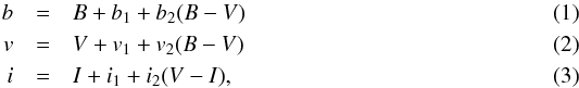 where BVI and bvi are the transformed APASS and instrumental magnitudes, respectively.
The calibration of infrared JHK data was performed on each cluster region using the information on common stars in the 2MASS catalog. To join the magnitudes obtained from the VVV images, we tried to use transformations using the form given by Soto et al. (2013). However we noticed, in some cases, a dependence on the residuals with stellar magnitude. Therefore we adopted the following dependencies:  where JHK and jhk are, respectively, 2MASS and instrumental VVV magnitudes.
The calibration coefficients of optical and infrared calibration equations were computed using the FITPARAMS task of IRAF PHOTCAL package. The values obtained are shown in Table 3.
To complete our data for saturated stars in VVV images, we simply adopted the 2MASS magnitudes for the brightest objects (K< 11).
Regarding the errors of our photometry for the BV and JHK bands, these can be estimated from their corresponding rms values, as obtained in the fittings (see Table 3) and complemented with the error values that were provided by DAOPHOT and DAOMASTER codes for each particular object (see Sect. 2.1.6). For the special case of I band, these errors must also be complemented with the system transformation error (~0.03; Jester et al. 2005).
Calibration coefficients used for optical and infrared observations.
2.1.5. Mid-infrared data
We cross-correlated our photometric data with mid-IR data (in the regions where these data are available) with the purpose of detecting PMS stars (see also Sect 3.4).
We then used, the MSX data (Egan et al. 2003) and SST data. MSX mapped the galactic plane and other regions that were missed or were identified as of particularly interest by the Infrared Astronomical Satellite (IRAS) at wavelengths of 4.29, 4.35, 8.28, 12.13, 14.65, and 21.3 μm. On the other hand, the Infrared Array Camera (IRAC) on board the SST was used to obtain images in four channels (3.6, 4.5, 5, 8, and 8.0 μm) and the GLIMPSE catalogue was produced using several of these photometric data points.
We the used then the all matches option in ALADIN since this option gave us all counterparts within the searching radius. Following these criteria, we found about ten counterparts in MSX and GLIMPSE data in each cluster region (see Sect. 4 for more details).
2.1.6. Final catalogs
We used the STILTS12 tool to manipulate tables and to cross-correlate the optical and IR data. We then obtained four catalogs with astrometric/photometric information of about 55 000 objects covering approximately a FOV of  around each cluster studied (see Fig. 1). The corresponding photometric errors (BVIJHK bands) in these catalogs are those provided by the DAOPHOT and DAOMASTER codes. The full catalogues (Tables 4a–d) are only available at the CDS.
2.2. Spectroscopic data
 |
Fig. 1 JHK false-color VVV images of the four regions studied. Selected clusters areas are indicated by big solid yellow circles. Comparison fields are also indicated with dotted circles in panels c) and d). Identified stars are those ones with NIR spectroscopy data or adopted brightest cluster members. Stars inside circles are adopted clusters members (see text and Table A.1). |
We performed spectroscopic observations on eight stars in the region of the embedded cluster DBS 77, which is distributed in three slit positions. We used the infrared spectrograph SofI13 on the NTT at La Silla Observatory ESO, Chile, in long-slit mode, during the night of 2011 April 17. Using the medium resolution grism in the 3rd order, we covered the whole KS band, 2.00–2.30 μm, with a resolution of Δλ4.66Å·pix-1. We used a 1 arcmin slit to match the seeing, which gives a resolving power of R ≃ 1320. For optimal subtraction of the atmospheric OH emission lines, we used 15 s (ID stars: 5; 8 and 3; slit 1); 100 s (ID stars: 17 and 27; slit 2) and 150 s (ID stars: 103; 21; and 39; slit 3) while nodding along the slit in an ABBA pattern: the star was observed before (A) and after (B) a first nod along the slit, then in position B a second time before returning to position A for a final exposure. The S/N for each spectrum is given in Table A.1. As a measure of atmospheric absorption, we observed bright stars of spectral type G. We used the standard procedures to reduce the data. For more details of our reduction procedures see Moorwood et al. (1998) and Chené et al. (2012, 2013).
2.3. Radio data
We consulted the HI SGPS data from the Australia Telescope Compact Array (ATCA) and the PMN survey that was carried out with the Parkes 64 m radio telescope and the NRAO seven-beam receiver with the aim of investigating the ISM in which star clusters are forming.
The SGPS is a survey of 21-cm HI spectral line emission and continuum. The HI data were obtained using a channel separation of Δv = 0.82 km s-1 and the final rms noise of a single profile is ~1.6 K on the brightness temperature (Tb) scale. The sensitivity of the radio continuum data is below 1 mJy beam-1 and the angular resolution of the SGPS is  .
.
The 21-cm HI spectral line survey provides data covering 253°≤l ≤ 358° and −1 5 ≤b ≤+15, and a small region in the first Galactic quadrant between 5°≤l ≤ 20° and −15 ≤b ≤+15 (SGPS I and SGPS II, respectively, see McClure-Griffiths et al. 2005 for details). The continuum survey only provides data for the 253°≤l ≤ 358° and −10 <b <+10 region (see Haverkorn et al. 2006 for details). We processed the SGPS continuum data using the NOD2 package (Haslam 1974).
The PMN is a southern sky survey at a frequency of ν = 4.8 GHz. The angular resolution is 5′ and the rms sensitivity is ~8 mJy beam -1. The survey provides several parameters (flux density, coordinates, angular size, orientation, etc.) of the H I distribution for −87° ≤ δ ≤ 10°.
3. Analysis
The methods employed to determine the fundamental parameters of the young stellar clusters, (sizes, extinctions, distances, ages, members, and masses) have already been described in several previous papers (see e.g., Chené et al. 2012, 2013; Baume et al. 2014). Here, we provide a brief summary and highlight what we did differently in this study.
3.1. Centers and sizes
The selected clusters are very faint and apparently have few members, which makes it difficult to apply the radial-density profile method. We then considered the coordinates that were given in the DBS catalog as the center coordinates as an initial point and for the visual inspection of the infrared images, together with the resulting photometric diagrams using different centers and radii. We finally adopted the values that contain the brightest stars and revealed the presence of the probable PMS population in the diagrams (see Table 1).
3.2. Kinematic study
Proper motions and radial velocities are very useful tools to assign cluster memberships. Unfortunately, the VVV database currently contains observations that cover four years and thus it is only possible to determine the proper motions for nearby Sun objects. On the other hand, the low-resolution of the spectra, combined with the small wavelength coverage, does not allow a very accurate measurement of the radial velocities. Consequently, our data were not reliable for providing membership probability from the kinematic behavior of the objects.
In this situation, we made use of kinematic information from HII regions, molecular and dark clouds projected at a distance of (~10′) from each cluster. We transformed their radial velocities (RV) referred to the local standard of rest (LSR) in kinematic distances. For this procedure we used the adjusted linear model (AL) and the law potential model (LP) given by Fich et al. (1989), or the Galactic rotation model of Brand & Blitz (1993) (see Sect. 4). The error in the determination of these kinematic distances arises because of an uncertainty of 10 km s-1 which is due to non-circular motion (Burton 1988). The HI maps, RV vs. b (Figs. 3 to 6), for each of the studied regions allowed us to resolve the distance-ambiguity problem present in the fourth Galactic quadrant. The kinematic distances that we obtained, provide a starting point for analyzing our photometric diagrams (see Sect. 3.4).
3.3. Spectrophotometric analysis
Spectrophotometric color excesses and distances were calculated for the stars for which we know their spectral classification from our spectra or from the bibliography. Our spectroscopic data include some of the brightest stars in the DBS 77 region and we used them to determine their spectral classification, verifying their cluster-membership situation. Spectral classification was performed using atlases of K-band spectra that feature spectral types stemming from optical studies (Rayner et al. 2009; Liermann et al. 2009; Meyer et al. 1998; Wallace & Hinkle 1997) (see Fig. 2).
We used the optical (BVI) and infrared (JHK) data and the calibrations given by Schmidt-Kaler (1982) and Koornneef (1983), respectively. Additionally, we evaluated the absorption values in the V and K bands as: AV = 3.1 EB − V and AK = 0.674 EJ − K, which are valid for a normal reddening law (see Sect. 3.4). For each cluster, we selected the stellar members where we are confident of their spectral type. We estimated individual stellar distances through the mean value of the computed V0 − MV and K0 − MK values.
3.4. Photometric diagrams
We checked the loci of the stars in all the possible color-magnitude diagrams and two-color diagrams (CMDs and TCDs, respectively) that were obtained from our catalog and located inside the adopted clusters regions (see adopted centers and radii for each cluster in Table 1). We present the corresponding diagrams in Figs. 7 to 10. Of note, optical data are available for all selected regions, except the DBS 160−161 region. These data were used to check a consistent fit of the MS over all the diagrams. To save space, we only present the optical diagrams for DBS 77 + VVV 16 regions. In general, the photometric diagrams reveal the presence of two stellar populations: a) the field population, usually late-type MS stars, represented by the group placed on the left in all the CMDs (gray symbols throughout the diagrams); and b) the cluster populations that experience high and differential reddening and mixed with possible field red giants. To separate both populations, we used (when available) the spectrophotometric analysis previously described, obtaining the corresponding color excesses and spectrophotometric distances. For stars without spectral classification, we used all the photometric diagrams and the reddening-free photometric parameter QNIR = (J − H) − 1.7(H − K) (Negueruela et al. 2007) to avoid the intrinsic degeneracy between reddening and spectral type. In particular, it was possible to use the (J − H) vs. (H − K) and/or the K vs. QNIR diagrams to distinguish different stellar populations.
 |
Fig. 2 Stellar spectra in the DBS 77 region. Several chemical components of each star are indicated with vertical lines. The spectral type of each star is indicated in Table A.1. |
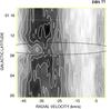 |
Fig. 3 Tb HI distribution at DBS 77 region (l ~ 301°). Black curved lines indicate the place of the HII region (RV = −46 km s-1) and the HI absorption in the line of sight. Lowest and highest contours are 12.4 K and 124 K, respectively. Contour spacing is 6 K until 50 K and 12 K from there onwards. Lighter gray color corresponds to the lowest temperature value. |
 |
Fig. 4 a) Same as for Fig. 3 but at DBS 78 region (l ~ 301°). Lowest and highest contours are 15 K and 152 K, respectively. Contour spacing is 15 K. b) Radio continuum emission at 1.42 GHz. Lowest and highest contours are 0.018 and 2.6 Jy beam-1, respectively, without a constant step. Lighter gray color corresponds to the lowest flux value. Dashed pattern circle drawn in the upper left-hand corner indicates the angular resolution of the HI data. |
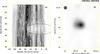 |
Fig. 5 a) Same as Fig.4 but at DBS 102 region (l ~ 333°). Here the HII region has RV = −52 km s-1. Lowest and highest contours are 30 K and 114 K, respectively. Contour spacing is 12 K. b) Lowest and highest contours in radio continuum emission are 0.1 and 2.7 Jy beam-1, respectively, without a constant step. |
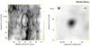 |
Fig. 6 a) Mean Tb HI distribution at DBS 160/161 region between the longitude range from |

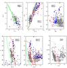 |
Fig. 7 Photometric diagrams for the stars in the DBS 77 + VVV 16 region and their corresponding comparison field (panel f)). Squares and circles represent stars with and without known spectral classification, respectively. Light gray symbols indicate a field population whereas blue and red represent different cluster populations selected by our photometric method (see text in Sect. 3.4). The solid (red) and dotted (green) curves are the ZAMS or MS (see text) shifted according to the distance modulus adopted with and without absorption/reddening, respectively. Dashed (red) lines indicate the normal reddening path (RV = 3.1). Dashed curves are Siess et al. (2000) isochrones for z = 0.02. |
In our procedure, we adopted as cluster members those stars that were placed approximately redder than an adopted consistent MS (red curve) along all the photometric diagrams. We adopted the MS calibrations given by Schmidt-Kaler (1982), Cousins (1978) and Koornneef (1983). Their locations were computed using the adopted distances and color excesses presented in Table 1 and a normal reddening behavior (see Sect. 3.3), as was suggested by the TCDs diagrams. This fact allowed us to use the absorption ratios (rX = AX/AV) given by Johnson (1968) van der Hulst curve 15 and Cambrésy et al. (2002). Then, following Borissova et al. (2012) and Messineo et al. (2012) we separated the selected stars among the early normal MS stars (−0.1 <QNIR< 0.15; blue symbols) and, stars with emission features or revealing IR excess (QNIR< −0.1; red symbols), including, for example, PMS stars and YSOs. We noticed that some spectroscopically confirmed OB stars in the DBS 77 and DBS 160 regions (see Figs. 7 and 10) have high QNIR values, but this could be a binarity effect. To confirm the reliability of our procedure, we conducted a similar analysis over a comparison field region for each cluster. In each case, as expected, we found almost no objects that could be considered as cluster members. We note, however, that we do not provide an unambiguous membership diagnostic, but we defined a uniform approach for selecting the likely member stars that were used to calculate the clusters parameters.
To estimate the absolute magnitudes and spectral types for the adopted MS cluster stars without spectroscopic observations, we de-reddened their location over the CMDs following a normal path until their intersection with the MS. In Table A.1, we present our adopted values and computations for stars studied with spectroscopic data and the more relevant ones (K< 13 or 14 depending on the cluster).
3.5. Individual stellar masses and IMF computation
We obtained the stellar mass for the adopted cluster members using the computed absolute magnitude values (see Sect. 3.4). We employed the ZAMS obtained from Bressan et al. (2012), Chen et al. (2014, 2015), Tang et al. (2014) and we interpolated the stellar mass using the algorithm given by Steffen (1990). This procedure is valid only for MS stars. For adopted PMS stars it only provides an approximate upper estimation of the real mass values.
The initial mass function (IMF) for massive stars can be modeled as a power law. This is  (7)where N is the number of stars per logarithmic mass bin Δ(log m). Since the computed spectral type depends upon the used photometric bands, we obtained several possible mass values for each star. Therefore, to build the IMF, we adopted the mean mass value obtained from Martins et al. (2005) for O-spectral types and, for B and later spectral types, from Pecaut & Mamajek (2013).
For each stellar group that we studied, we built two IMFs, taking only the adopted MS stars into account and adding the adopted PMS stars. We note that the uncertainly in their mass values was minimized by the width of the bins used in the IMF estimation. Our results are presented in Fig. 11, together with the least-squares fit for the most massive stars (>3 M⊙), avoiding the very probably incomplete less massive bins. We noticed that, except in the case of the DBS 77 region, the presence of PMS has a significant effect on the obtained slope values (see Table 1 and Fig. 11).
3.6. Estimating cluster ages
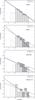 |
Fig. 11 Distribution of stellar masses for the embedded clusters studied. Gray bars (light and dark) indicate more massive bins employed to compute the IMF slopes (Γ). Light gray bars and blue solid lines refer only to MS stars, whereas dark gray bars and black dashed lines refer to MS+PMS stars. |
Since all the clusters presented strong differential reddening, it was very difficult to estimate their ages using the classical method of fitting the observed CMD with isochrone sets. We therefore took the early spectral type of the stars adopted as cluster members into account and the Ekström et al. (2012) evolutionary models to calculate the MS duration from the mass of the star. When spectroscopic data were not available, we used the estimated spectral classification from the photometric data (see Sect. 3.4 and Table A.1). We note that the estimated age values are upper limits since the high amount of PMS candidates that were revealed suggest an active star formation process in all the clusters studied.
3.7. Studying the radio maps
Main parameters of the HII regions linked with the embedded clusters studied.
The selected radio data (see Sect. 2.3) provide HI spectral line information over all the selected regions but, unfortunately, the continuum survey only provides data until b = 1°. For this reason we could not analyze the HI distribution at 1.4 GHz for DBS 77 region. We derived the angular diameters and flux densities (Sν) of the radio continuum point sources found in the direction of DBS 160−161 and DBS 78 using a bidimenssional gaussian fit to the SGPS continuum data. The error in the fit was about 2% and we determined a rms flux noise level of 0.013 Jy beam-1 from a source-free region located in the neighborhood. The fitted parameters that we obtained are presented in Table 5.
In the direction of DBS 102 we found an extended source (for the angular resolution of the SGPS survey), with an angular size of 7 3 × 69. We calculated the integrated flux density of the source using the method of polygon integrations and we subtracted the background with a lineal baseline fit. The quoted error reflected the uncertainties in determining the background levels, which added up to a total of about 5%.
The emission mechanism of the radio sources detected could be identified using the spectral index α (S ~ ν− α). This index was obtained from the measured flux density at two different frequencies, ν1 and ν2 (α = log (S1/S2) / log (ν2/ν1)). We computed the corresponding spectral indices for the radio sources found in the direction of the clusters DBS 78, DBS 102, and DBS 160−161 using the SGPS data (1.4 GHz) and the PMN data (4.85 GHz). The α ≃ 0.1 values found with both frequencies revealed a spectra whose behavior was as expected for an optically thin plasma. The values obtained are presented in Table 5.
The bidimensional gaussian fit and the method of polygon integration (for point or extended sources, respectively) also provided the peak brightness temperature (TC) for each source at 1.4 GHz. The parameter (TC), for these regions, was also computed by Brown et al. (2014) obtaining different values, however they employed the “on-off method” (see Kolpak et al. 2003). The TC values obtained by us and by Brown et al. (2014) are shown in Table 5.
The analysis of the observations in the radio continuum spectrum of the optically thin nebula enabled us to estimate the excitation parameter ![Mathematical equation: \hbox{${\it u}\,[{\rm pc\,cm}^{-2}]= R_{\rm s} N^{2/3}_{\rm e}$}](/articles/aa/full_html/2016/04/aa26121-15/aa26121-15-eq182.png) . This value represents the Lyman photon number that might be absorbed by the H region to be ionized and become in one HII region. The linear Strömgren radio, Rs, was obtained as the geometric mean of the angular size of the source and Ne is the electronic density. This latter value was computed for each region using a geometric model and employing the expression given by Mezger & Henderson (1967):
. This value represents the Lyman photon number that might be absorbed by the H region to be ionized and become in one HII region. The linear Strömgren radio, Rs, was obtained as the geometric mean of the angular size of the source and Ne is the electronic density. This latter value was computed for each region using a geometric model and employing the expression given by Mezger & Henderson (1967): ![Mathematical equation: \begin{eqnarray} \label{Ne} \nonumber N_{\rm e}[{\rm cm}^{-3}] &=& c_1 a^{1/2} 635.1 (T_{\rm e} [10^4~{\rm k}])^{0.175} (\nu[{\rm GHz}])^{0.05} (S_{\nu}[{\rm Jy}])^{1/2}\\ &&\quad \times (1/d[{\rm kpc}])^{1/2}(\theta_{\rm G}[{\rm arc min}])^{-1.5}, \end{eqnarray}](/articles/aa/full_html/2016/04/aa26121-15/aa26121-15-eq184.png) (8)where c1 = 0.775 is the conversion factor employed for the spheric geometric model adopted for the nebula, a = 1 is the recombination coefficient at all levels, Te is the electronic temperature obtained from the model of Quireza et al. (2006), Sν is the flux density measured in the HII region at ν = 1.42 GHz and θG is the observed apparent half-power beam width (HPBW), obtained as
(8)where c1 = 0.775 is the conversion factor employed for the spheric geometric model adopted for the nebula, a = 1 is the recombination coefficient at all levels, Te is the electronic temperature obtained from the model of Quireza et al. (2006), Sν is the flux density measured in the HII region at ν = 1.42 GHz and θG is the observed apparent half-power beam width (HPBW), obtained as  (9)with θsph1 and θsph2 being the geometric mean of the observed size of the source in two perpendicular coordinates.
Moreover, using models of stellar atmospheres, it is possible to determine the total number (NLy) of ionizing photons in the Lyman continuum of the hydrogen that is emitted by the exciting star. We adopted the NLy values given by Smith et al. (2002). They calculated non-LTE, line-blanketed model atmospheres for several metallicities that cover the entire upper Hertzprung-Russell diagram for massive stars with stellar winds. We then computed NLy for adopted cluster members stars earlier than B 2.0, since they provide almost all these photons.
Thus, the ionization parameter could be calculated as ![Mathematical equation: \begin{eqnarray} \label{photons} U\,[{\rm pc\,cm}^{-2}] = [3 N_{\rm Ly} / 4 \pi a(2)]^{1/3}, \end{eqnarray}](/articles/aa/full_html/2016/04/aa26121-15/aa26121-15-eq193.png) (10)where a(2) = 2.76 × 10⁻¹³ [ cm3 s-1 ] represents the probability of recombination at all levels except the ground level. We then compared the excitation parameter u with the parameter U calculated with Eq. (10) for all the exciting stars. Thus, we compared the observational results of density and radius of the nebula with the flow of ionizing photons emitted by the exciting stars. The comparison enabled us to determine whether the HII region deviates from the ideal conditions and what might be the causes. The obtained results of these comparisons are discussed in Sect. 5.2 and are presented in Table 5.
(10)where a(2) = 2.76 × 10⁻¹³ [ cm3 s-1 ] represents the probability of recombination at all levels except the ground level. We then compared the excitation parameter u with the parameter U calculated with Eq. (10) for all the exciting stars. Thus, we compared the observational results of density and radius of the nebula with the flow of ionizing photons emitted by the exciting stars. The comparison enabled us to determine whether the HII region deviates from the ideal conditions and what might be the causes. The obtained results of these comparisons are discussed in Sect. 5.2 and are presented in Table 5.
An optically thin HII region also allowed us to estimate the mass of ionized hydrogen in the region following the expression given by Mezger & Henderson (1967): ![Mathematical equation: \begin{eqnarray} \label{MHII} \nonumber M_{\rm H\,II}[M_\odot] &=& c_2 a^{1/2}\! 0.3864 (T_{\rm e} [10^4~{\rm k}])^{0.175} (\nu[{\rm GHz}])^{0.05} \!(S_{\nu}[{\rm Jy}])^{1/2}\\ &&\quad \times (d[{\rm kpc}])^{2.5}(\theta_G[{\rm arc min}])^{1.5}, \end{eqnarray}](/articles/aa/full_html/2016/04/aa26121-15/aa26121-15-eq195.png) (11)where c2 = 1.291 is the conversion factor employed for the spheric geometric model adopted for the nebula, and the other observable quantities are the same as those used in Eq. (8).
(11)where c2 = 1.291 is the conversion factor employed for the spheric geometric model adopted for the nebula, and the other observable quantities are the same as those used in Eq. (8).
The 21-cm line emission maps of the studied regions (see Figs. 3 to 6) show zones with low values of Tb. For DBS 77, DBS 78, and DBS 102 regions, these minima could be interpreted as the result of the absorption of the HI distribution, which indicates that Tc>Tb. On the other hand, the DBS 160−161 region presents a minimum in the HI emission distribution surrounded by enhanced HI emission, revealing the presence of a bubble. Interstellar bubbles are cavities with a minimum in the center of its HI distribution, which is expanding at relatively low velocities (≤10 km s-1) (Cappa et al. 2003).
4. Describing clusters regions
4.1. DBS 77, VVV 15, and VVV 16
Since these three clusters are placed at the same studied region and their photometric diagrams revealed similar properties, they were only studied as one stellar group. We performed spectral classification of eight stars in this region (see Sect. 2.2), determining that three of them could be considered cluster members and gave us a spectrophotometric distance of 4.6 kpc (see Table 1). The 21-cm line emission map in this region (see Fig. 3) shows that the largest HI absorption signature corresponds with a velocity value of −46 km s-1. The value in this Galactic region has no distance associated with the kinematic rotation models of the Galaxy (see Fig. 11), which means that this velocity is a “forbidden value” for these models and that the perturbations of the rotation of the Galaxy could be causing it. The radial velocity of the region, according to the Brand & Blitz (1993) model would be approximately −33 km s-1, which corresponds to the tangential point that is linked to a distance of ≃4.6 ± 0.5 kpc. This value is similar to the spectrophotometric one previously indicated and is consistent with other kinematic determinations (Fich et al. 1989; Bronfman et al. 1996). We therefore adopted 4.6 kpc as the most reliable distance for the studied stellar group in this region.
Our photometric analysis indicated the presence of an important amount of early MS stars (four O-type stars and 40 B-type stars) and 13 probable PMS stars. In this region we found six MSX source candidates to YSOs, (Mottram et al. 2007) with eight possible IR counterparts.
We could not calculate the excitation parameter u of this region because there are no maps with HI emission distribution data in the continuum at 1.4 GHz for this region.
4.2. DBS 78
There are no stars with spectral classification in this region, so we employed the 21-cm HI emission of the DBS 78 region to obtain its kinematic distance (see Fig. 4). We found that the largest HI absorption signature corresponds with a velocity value of −46 km s-1 (near to −41 km s-1, as given by Bronfman et al. 1996). The regions of DBS 77 and DBS 78 are relatively near (~15′) in the same location of the Galaxy so, for DBS 78, we used the same rotation curves as in the previous case (see Fig. 12) and we therefore also adopted the same distance value (4.6 kpc).
The corresponding photometric diagrams reveal that DBS 78 is experiencing a stronger absorption than DBS 77 (see Table 1). Our photometric analysis indicated the presence of 15 B-type stars and ~20 probable PMS stars for DBS 78. In the region of this cluster there are two GLIMPSE sources with three possible IR counterparts and one MSX source with four possible IR counterparts.
 |
Fig. 12 Galactic rotation models applied at l = 301° to our Galaxy. The arrow indicates the adopted distance to the radial velocity of the radio sources according to the model. |
4.3. DBS 102
In this instance, we analyzed our photometric data centering on two regions:
-
DBS 102a: this region is centered at the coordinates given for Dutra et al. (2003) for the cluster and is also associated with IRAS source 16112-4943.
-
DBS 102b: this region is centered near the location of MSX6C G333.0058+00.7707 and IRAS 16115-4941 sources where JHK images revealed the presence of a small HII region.
Since there are not available stars with spectral classification in these regions, we employed the 21-cm HI emission of the DBS 102 region to obtain the kinematic distance. We adopted the distance provided for the Galactic kinematic models using Fich et al. (1989) data. As can be seen in Fig. 5, that the main HI absorption feature in this line of sight is present from ≃−52 km s-1 to 0 km s-1. The former value is consistent with that associated with the HII region G333.0+0.8 given by Kuchar & Clark (1997). In this way it was possible to resolve the ambiguity in distance of the adopted kinematic model and to assign a kinematic distance of 3.6 ± 0.4 kpc. If the HII region would be at the other distance (≃12 kpc) that was obtained with this rotation model of the Galaxy, HI absorption would have to be observed at radial velocity values lower than −60 km s-1 and this is not the case.
Applying our photometric analysis, we could identify one O-type star, nine B-type stars and approximately 13 PMS stars in all 102 DBS region. There are eight GLIMPSE sources with nine possible IR counterparts.
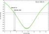 |
Fig. 13 Galactic rotation models applied at l = 333° to our Galaxy. Arrows indicate the corresponding distance to the radial velocity of the radio sources according to the model. |
4.4. DBS 160 and DBS 161
Working with the MS stars in the region that have spectral classification (Roman-Lopes et al. 2009), we obtained a spectrophotometric distance of 2.9 kpc, which is consistent with the kinematic one obtained by Fich et al. (1989) data (3 ± 0.3 kpc) and close to the spectrophotometric mean value of 2.4 ± 0.5 kpc that was obtained by Roman-Lopes et al. (2009). The analysis of the Galactic rotation curve is similar to that performed for the DBS 102 region.
Our photometric study revealed one O-type star, 28 B-type stars and approximately 20 PMS stars for both clusters, DBS 160 and DBS 161. Thus, in the whole DBS 160−161 region we found fewer OB-type stars than Roman-Lopes & Abraham (2004). They indicated the presence of three O-type stars and 55 B-type stars. Probably, this difference is the consequence of the spectral classification that was performed with photometric analysis.
The HI emission in this region (see Fig. 6a) revealed the presence of a bubble located at (RV,b) ~ (−42 km s-1,−0.̊14). Figure 14b shows a cross-cut of Fig. 6a along b = −0.̊14, where the presence of two peaks in the Tb at −45.9 (vm) and −38 (vM) km s-1 could be observed, which defines the walls of the bubble. Based on the assumption of a symmetric expansion of the bubble, it will attain its maximum dimension at the systemic velocity (v0). The value of v0 corresponds to the velocity between the two peaks where the minimum value of Tb is observed. At intermediate velocities the dimension of the bubble shrinks as vM (or vm) is approached. The expansion velocity (vexp) is estimated as half the total velocity range (vexp = 0.5 | vM − vm |) covered by the HI emission that is related to the feature. Figure 14a shows the HI emission distribution in the velocity range from −44.5 to −40.4 km s-1, where the bubble is easily recognizable. We will refer to this bubble as B332.5−0.1−42.
To estimate the main physical parameters of B332.5−0.1−42, we characterized the ellipse obtained from the least-squares fit to the local maxima around the cavity. The parameters derived from this fit were the symmetry center of the ellipsoidal HI distribution (l0,b0), the length of both the semi-major (a) and semi-minor (b) axes of the ellipse, and the inclination angle (φ) between the major axis and the galactic longitude axis (measured positively toward the north Galactic pole).
We also estimated the total gaseous mass associated with B332.5−0.1−42 as MH I [ gr ] = NH I [ cm-2 ] mH I [ gr ] AH I [ cm2 ], where NH I is the H I column density,  , and AH I is the area covered by the bubble, which was computed from the solid angle covered by the structure at the adopted distance to the Sun. Adopting solar abundances, the total gaseous mass of the bubble is Mt = 1.34 MHI.
Another important parameter that characterizes the bubble is its kinetic energy, which is given by ![Mathematical equation: \hbox{$E_k [{\rm erg}] = 0.5\,M_{\rm t}[{\rm gr}]\, v^2_{\exp}[{\rm cm}^2\,{\rm s}^{-2}]$}](/articles/aa/full_html/2016/04/aa26121-15/aa26121-15-eq223.png) . The dynamic age of the bubble could be estimated from tdyn [ Myr ] = αRef [ pc ] /vexp [ km s-1 ], where α = 0.6 for a stellar wind bubble (Weaver et al. 1977).
. The dynamic age of the bubble could be estimated from tdyn [ Myr ] = αRef [ pc ] /vexp [ km s-1 ], where α = 0.6 for a stellar wind bubble (Weaver et al. 1977).
All the parameters computed for the bubble B332.5−0.1−42 are presented in Table 6 in self-explanatory format.
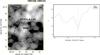 |
Fig. 14 DBS 160−161: a) Mean Tb of the H I emission distribution associated with the B332.5−0.1−42 in the velocity range from −44.5 to −40.4 km s-1. Contour levels are from 80 to 110 K in steps of 5 K. Best-fitted ellipse to the bubble is indicated with dashed lines and the circle inside it indicates the ultra compact HII region GRS332.5−00.10. b) H I brightness temperature profile along |

Main parameters of the B332.5−0.1−42.
5. Specific discussions
5.1. Was the HI bubble (B332.5−0.1−42) created by the stars of DBS 160 and DBS 161 clusters?
According with our analysis, it seems that the clusters DBS 160−161 are located inside the bubble B332.5−0.1−42. Is it possible that these stars could have created the bubble with their winds? To answer this question we calculated the total mechanical energy (Ew) injected by each star in the course of its entire evolutionary stage. This value was estimated as EW = Lwτ, where τ is the age of the star and Lw is the stellar mechanical luminosity (Lw = 0.5 Mv ), which was obtained from the stellar mass loss rate (Ṁ) and the wind terminal velocity (v∞). We estimated these latter two parameters by using the atmosphere models derived by Vink et al. (2001). They predict the rate at which mass is lost due to stellar winds from massive O- and B-type stars as a function of metal abundance. We employed the results presented in their Table 3 using solar metallicity and the corresponding Teff for each star that were assigned by Schmidt-Kaler (1982) from spectral classification.
The stellar mass for each spectral type was obtained according to the analysis developed in Sect. 3.5. In these computations, we adopted a model of a single stellar population for the massive cluster stars. Therefore, the estimated age of the cluster could be considered as the same value (τ) for the whole cluster’s brightest members (MS stars). As a result, we obtained an upper limit for the total mechanical energy injected by the cluster stars into the ISM. To avoid field stellar contamination of the cluster stars, we applied the above procedure to the stars located in the clusters region and to the stars in the adopted comparison field to compute the total energy, and finally we subtracted both results. Thus the net total mechanical energy was (1.43 ± 0.52) × 1050 erg.
The theoretical models predict that only 20% of the wind-injected energy is converted into mechanical energy of an expanding shell (Weaver et al. 1977). The energy conversion efficiency seems to be as low as 2–5% (Cappa et al. 2003) from an observational viewpoint. In this way, the energy used to originate the bubble may have been (2.9 or 7.1) × 1048 erg.
Both these values are greater than the kinetic energy that would actually have generated the G332.5−0.1−42 bubble. With this result, the stars possible members of DBS 160 and DBS 161 clusters could have generated the bubble.
5.2. The evolutionary state of the studied HII regions
All the embedded clusters analyzed in this paper share their location in the Galaxy with HII regions. For DBS 77, DBS 102ab and DBS 160−161 clusters, we obtained that U>u, so, the neutral gas cloud where the HII region is immersed is completely ionized, therefore the region is limited by density. Beyond this material, there is no ionizable material or there is dust mixed with the ionized gas that absorbs the UV photons emitted by the cluster stars and then re-emits them in the IR wavelength. The photons are consumed and are not useful to ionize the gas, resulting only in an increase in temperature of the interstellar dust. This result proves that the short formation phase during which the central cluster rapidly ionizes the neutral medium is over. Therefore, all the studied HII regions are in a long expansion phase, where the pressure in the warm ionized gas (Te ~ 104 K, see Table 5) is higher than Tb in the cold neutral medium that surrounds the HII regions (Tb ≤ 150 K). In this way, the electron density of the HII regions will decrease.
For DBS 78 we found that U<u, therefore the region is limited by ionization. That is, part of the gas that surrounds the embedded cluster has been ionized by exciter stars and the other part of the gas has not yet been ionized. This may be due to the absence in the cluster of O-type stars, or by not considering the Lyman photon emission that is produced by the PMS stars, which are present in DBS 78.
The infrared emission from dust around developed HII regions present a strong case that most HII regions do form inside dusty HI regions. A small HII region develops around the star, probably with material rather denser than average for the cloud, owing to the local concentration that produced the star initially.
6. Conclusions
We studied the embedded clusters DBS 77, 78, 102, 160, and 161 that were positioned behind dust clouds in the fourth quadrant of the Vía Láctea. We grouped these clusters into four regions according to their spatial location and we computed their fundamental parameters, revealing the nature of their brightest members and the probable presence of PMS stars in all of them (see Tables 1 and A.1 for details).
We found that the DBS 160−161 clusters are located inside the HI bubble, referred to by us as B332.5−0.1−42, and we estimated the main parameters of this bubble (see Table 6 for details). The stellar winds of DBS 160−161 clusters members may well have been the creators of B332.5−0.1−42.
We also obtained the IMF for massive star members for each cluster. The slope value obtained for DBS 77 cluster (Γ = −1.44) was similar to Γ = −1.35 given by Salpeter (1955). The slope values obtained for the DBS 160−161 clusters (Γ = −0.71), for DBS 102ab (Γ = −0.75) and for DBS 78 (Γ = −1.19), were a little less steep than the Salpeter (1955) value. This behavior was also found in some young stellar clusters (see Baume et al. 2003) and could be a signature for this type of object.
In addition to the clusters mentioned above, we studied the HII regions that are associated with each of them. We estimated the main parameters of these HII regions (see Table 5). We computed their mean LSR radial velocity (RV(LSR)) to obtain a kinematic distance and to compare their values with spectrophotometric ones. With regard to the angular diameter, θsph, we were able to identify that the HII region in the DBS 102 cluster was an extended one. We were also able to estimate the excitation parameter u of each HII region and the ionization parameter U of each cluster that is linked to these H II regions. The comparison of u with U is a basic tool in the study of relations between HII regions and exciting stars. We found that the regions that are linked to the embedded clusters DBS 77, DBS 102ab, and DBS 160−161 are limited by density. This result indicates that the central cluster has already ionized all the interstellar material and the HII regions we studied are in a long expansion phase, where the pressure in the warm ionized gas is higher than the equivalent in the cold neutral medium that surrounds the H II regions. The region linked to the embedded cluster DBS 78 is limited by ionization. This result indicates that, at the moment, only a part of the region has been ionized.
IRAF is distributed by NOAO, which is operated by AURA under cooperative agreement with the NSF.
Acknowledgments
M.A.C., G.L.B., J.A.P., L.A.S. y J.C.T. acknowledge support from CONICET (PIPs 112-201201-00226 y 112-201101-00301). The authors are much obliged for the use of the NASA Astrophysics Data System, of the SIMBAD database and ALADIN tools (Centre de Donnés Stellaires – Strasbourg, France). This publication also made use of data from: a) the Two Micron All Sky Survey, which is a joint project of the University of Massachusetts and the Infrared Processing and Analysis Center/California Institute of Technology, funded by the National Aeronautics and Space Administration and the National Science Foundation; b) the AAVSO Photometric All-Sky Survey (APASS), funded by the Robert Martin Ayers Sciences Fund; c) the Midcourse Space Experiment (MSX). Processing of the data was funded by the Ballistic Missile Defense Organization, with additional support from NASA Office of Space Science. Support for J.B., S.R.A., and R.K. is provided by the Ministry of Economy, Development, and Tourism’s Millennium Science Initiative through grant IN 120009, awarded to The Millennium Institute of Astrophysics, MAS. J.B. is supported by FONDECYT No.1120601, R.K. is supported by Fondecyt Reg. No. 1130140, SRA by Fondecyt No. 3140605. We thank R. Martínez and H. Viturro for technical support and E. Marcelo Arnal for many useful comments which improved this paper. Finally, we wish to thank the anonymous referee for their suggestions and comments, which improved the original version of this work.
References
- Bains, I., Wong, T., Cunningham, M., et al. 2006, MNRAS, 367, 1609 [NASA ADS] [CrossRef] [Google Scholar]
- Barba, R. H., Roman-Lopes, A., Nilo Castellon, J. L., et al. 2015, A&A, 581, A120 [NASA ADS] [CrossRef] [EDP Sciences] [Google Scholar]
- Baume, G., Vázquez, R. A., Carraro, G., & Feinstein, A. 2003, A&A, 402, 549 [NASA ADS] [CrossRef] [EDP Sciences] [Google Scholar]
- Baume, G., Carraro, G., & Momany, Y. 2009, MNRAS, 398, 221 [NASA ADS] [CrossRef] [Google Scholar]
- Baume, G., Rodríguez, M. J., Corti, M. A., Carraro, G., & Panei, J. A. 2014, MNRAS, 443, 411 [NASA ADS] [CrossRef] [Google Scholar]
- Borissova, J., Bonatto, C., Kurtev, R., et al. 2011, A&A, 532, A131 [NASA ADS] [CrossRef] [EDP Sciences] [Google Scholar]
- Borissova, J., Georgiev, L., Hanson, M. M., et al. 2012, A&A, 546, A110 [NASA ADS] [CrossRef] [EDP Sciences] [Google Scholar]
- Borissova, J., Chené, A.-N., Ramírez Alegría, S., et al. 2014, A&A, 569, A24 [NASA ADS] [CrossRef] [EDP Sciences] [Google Scholar]
- Brand, J., & Blitz, L. 1993, A&A, 275, 67 [NASA ADS] [Google Scholar]
- Bressan, A., Marigo, P., Girardi, L., et al. 2012, MNRAS, 427, 127 [NASA ADS] [CrossRef] [Google Scholar]
- Bronfman, L., Nyman, L.-A., & May, J. 1996, A&AS, 115, 81 [NASA ADS] [Google Scholar]
- Brown, C., Dickey, J. M., Dawson, J. R., & McClure-Griffiths, N. M. 2014, ApJS, 211, 29 [NASA ADS] [CrossRef] [Google Scholar]
- Burton, W. B. 1988, in Galactic and Extragalactic Radio Astronomy (Springer-Verlag), 295 [Google Scholar]
- Cambrésy, L., Beichman, C. A., Jarrett, T. H., & Cutri, R. M. 2002, AJ, 123, 2559 [NASA ADS] [CrossRef] [Google Scholar]
- Cappa, C. E., Arnal, E. M., Cichowolski, S., Goss, W. M., & Pineault, S. 2003, in A Massive Star Odyssey: From Main Sequence to Supernova, eds. K. van der Hucht, A. Herrero, & C. Esteban, IAU Symp., 212 [Google Scholar]
- Chen, Y., Girardi, L., Bressan, A., et al. 2014, MNRAS, 444, 2525 [NASA ADS] [CrossRef] [Google Scholar]
- Chen, Y., Bressan, A., Girardi, L., et al. 2015, MNRAS, 452, 1068 [NASA ADS] [CrossRef] [Google Scholar]
- Chené, A.-N., Borissova, J., Clarke, J. R. A., et al. 2012, A&A, 545, A54 [NASA ADS] [CrossRef] [EDP Sciences] [Google Scholar]
- Chené, A.-N., Borissova, J., Bonatto, C., et al. 2013, A&A, 549, A98 [NASA ADS] [CrossRef] [EDP Sciences] [Google Scholar]
- Cousins, A. W. J. 1978, The Observatory, 98, 54 [NASA ADS] [Google Scholar]
- Dobashi, K. 2011, PASJ, 63, 1 [NASA ADS] [CrossRef] [Google Scholar]
- Dutra, C. M., Bica, E., Soares, J., & Barbuy, B. 2003, A&A, 400, 533 [NASA ADS] [CrossRef] [EDP Sciences] [Google Scholar]
- Egan, M. P., Price, S. D., Kraemer, K. E., et al. 2003, VizieR Online Data Catalogs: V/114 [Google Scholar]
- Ekström, S., Georgy, C., Eggenberger, P., et al. 2012, A&A, 537, A146 [NASA ADS] [CrossRef] [EDP Sciences] [Google Scholar]
- Fich, M., Blitz, L., & Stark, A. A. 1989, ApJ, 342, 272 [NASA ADS] [CrossRef] [Google Scholar]
- Haslam, C. G. T. 1974, A&AS, 15, 333 [NASA ADS] [Google Scholar]
- Haverkorn, M., Gaensler, B. M., McClure-Griffiths, N. M., Dickey, J. M., & Green, A. J. 2006, ApJS, 167, 230 [CrossRef] [Google Scholar]
- Henden, A. A., Terrell, D., Welch, D., & Smith, T. C. 2010, BAAS, 42, 515 [NASA ADS] [Google Scholar]
- Jester, S., Schneider, D. P., Richards, G. T., et al. 2005, AJ, 130, 873 [NASA ADS] [CrossRef] [Google Scholar]
- Johnson, H. L. 1968, in Nebulae and interstellar matter, eds. B. M. Middlehurst, & L. H. Aller (University of Chicago Press), 167 [Google Scholar]
- Kharchenko, N. V., Piskunov, A. E., Röser, S., Schilbach, E., & Scholz, R.-D. 2005, A&A, 438, 1163 [NASA ADS] [CrossRef] [EDP Sciences] [MathSciNet] [Google Scholar]
- Kolpak, M. A., Jackson, J. M., Bania, T. M., Clemens, D. P., & Dickey, J. M. 2003, ApJ, 582, 756 [NASA ADS] [CrossRef] [Google Scholar]
- Koornneef, J. 1983, A&A, 128, 84 [NASA ADS] [Google Scholar]
- Kuchar, T. A., & Clark, F. O. 1997, ApJ, 488, 224 [NASA ADS] [CrossRef] [Google Scholar]
- Lequeux, J. 2005, The Interstellar Medium (Berlin: Springer) [Google Scholar]
- Liermann, A., Hamann, W.-R., & Oskinova, L. M. 2009, A&A, 494, 1137 [NASA ADS] [CrossRef] [EDP Sciences] [Google Scholar]
- Martins, F., Schaerer, D., & Hillier, D. J. 2005, A&A, 436, 1049 [NASA ADS] [CrossRef] [EDP Sciences] [Google Scholar]
- McClure-Griffiths, N. M., Dickey, J. M., Gaensler, B. M., et al. 2005, ApJS, 158, 178 [NASA ADS] [CrossRef] [Google Scholar]
- Messineo, M., Menten, K. M., Churchwell, E., & Habing, H. 2012, A&A, 537, A10 [NASA ADS] [CrossRef] [EDP Sciences] [Google Scholar]
- Meyer, M. R., Edwards, S., Hinkle, K. H., & Strom, S. E. 1998, ApJ, 508, 397 [NASA ADS] [CrossRef] [Google Scholar]
- Mezger, P. G., & Henderson, A. P. 1967, ApJ, 147, 471 [NASA ADS] [CrossRef] [Google Scholar]
- Minniti, D., Lucas, P. W., Emerson, J. P., et al. 2010, New A, 15, 433 [Google Scholar]
- Moorwood, A., Cuby, J.-G., & Lidman, C. 1998, The Messenger, 91, 9 [NASA ADS] [Google Scholar]
- Mottram, J. C., Hoare, M. G., Lumsden, S. L., et al. 2007, A&A, 476, 1019 [NASA ADS] [CrossRef] [EDP Sciences] [Google Scholar]
- Negueruela, I., Marco, A., Israel, G. L., & Bernabeu, G. 2007, A&A, 471, 485 [NASA ADS] [CrossRef] [EDP Sciences] [Google Scholar]
- Pecaut, M. J., & Mamajek, E. E. 2013, ApJS, 208, 9 [NASA ADS] [CrossRef] [Google Scholar]
- Peretto, N., & Fuller, G. A. 2009, A&A, 505, 405 [NASA ADS] [CrossRef] [EDP Sciences] [Google Scholar]
- Pinheiro, M. C., Abraham, Z., Copetti, M. V. F., et al. 2012, MNRAS, 423, 2425 [NASA ADS] [CrossRef] [Google Scholar]
- Quireza, C., Rood, R. T., Bania, T. M., Balser, D. S., & Maciel, W. J. 2006, ApJ, 653, 1226 [NASA ADS] [CrossRef] [Google Scholar]
- Rayner, J. T., Cushing, M. C., & Vacca, W. D. 2009, ApJS, 185, 289 [NASA ADS] [CrossRef] [Google Scholar]
- Robitaille, T. P., Meade, M. R., Babler, B. L., et al. 2008, AJ, 136, 2413 [NASA ADS] [CrossRef] [Google Scholar]
- Roman-Lopes, A., & Abraham, Z. 2004, AJ, 127, 2817 [NASA ADS] [CrossRef] [Google Scholar]
- Roman-Lopes, A., Abraham, Z., Ortiz, R., & Rodriguez-Ardila, A. 2009, MNRAS, 394, 467 [NASA ADS] [CrossRef] [Google Scholar]
- Russeil, D., & Castets, A. 2004, A&A, 417, 107 [NASA ADS] [CrossRef] [EDP Sciences] [Google Scholar]
- Saito, R. K., Hempel, M., Minniti, D., Lucas, P. W., & et al. 2012, A&A, 537, A107 [NASA ADS] [CrossRef] [EDP Sciences] [Google Scholar]
- Salpeter, E. E. 1955, ApJ, 121, 161 [Google Scholar]
- Schmidt-Kaler, Th. 1982, In Landolt-Bornstein New Series, Group VI, Vol. 2b, eds. K. Schaifers, & H. H. Voigt (Berlin: Springer-Verlag) [Google Scholar]
- Siess, L., Dufour, E., & Forestini, M. 2000, A&A, 358, 593 [Google Scholar]
- Skrutskie, M. F., Cutri, R. M., Stiening, R., et al. 2006, AJ, 131, 1163 [NASA ADS] [CrossRef] [Google Scholar]
- Smith, L. J., Norris, R. P. F., & Crowther, P. A. 2002, MNRAS, 337, 1309 [NASA ADS] [CrossRef] [Google Scholar]
- Soto, M., Barbá, R., Gunthardt, G., et al. 2013, A&A, 552, A101 [NASA ADS] [CrossRef] [EDP Sciences] [Google Scholar]
- Steffen, M. 1990, A&A, 239, 443 [NASA ADS] [Google Scholar]
- Stetson, P. B. 1987, PASP, 99, 191 [NASA ADS] [CrossRef] [Google Scholar]
- Stetson, P. B. 1992, in Astronomical Data Analysis Software and Systems I, eds. D. M. Worrall, C. Biemesderfer, & J. Barnes, ASP Conf. Ser., 25, 297 [Google Scholar]
- Tang, J., Bressan, A., Rosenfield, P., et al. 2014, MNRAS, 445, 4287 [NASA ADS] [CrossRef] [Google Scholar]
- Vink, J. S., de Koter, A., & Lamers, H. J. G. L. M. 2001, A&A, 369, 574 [NASA ADS] [CrossRef] [EDP Sciences] [Google Scholar]
- Wallace, L., & Hinkle, K. 1997, ApJS, 111, 445 [NASA ADS] [CrossRef] [Google Scholar]
- Weaver, R., McCray, R., Castor, J., Shapiro, P., & Moore, R. 1977, ApJ, 218, 377 [NASA ADS] [CrossRef] [Google Scholar]
Appendix A: Additional table
Adopted photometric data and spectral classification for the most relevant stars in each region studied.
All Tables
Adopted photometric data and spectral classification for the most relevant stars in each region studied.
All Figures
|
Fig. 1 JHK false-color VVV images of the four regions studied. Selected clusters areas are indicated by big solid yellow circles. Comparison fields are also indicated with dotted circles in panels c) and d). Identified stars are those ones with NIR spectroscopy data or adopted brightest cluster members. Stars inside circles are adopted clusters members (see text and Table A.1). |
| In the text | |
|
Fig. 2 Stellar spectra in the DBS 77 region. Several chemical components of each star are indicated with vertical lines. The spectral type of each star is indicated in Table A.1. |
| In the text | |
|
Fig. 3 Tb HI distribution at DBS 77 region (l ~ 301°). Black curved lines indicate the place of the HII region (RV = −46 km s-1) and the HI absorption in the line of sight. Lowest and highest contours are 12.4 K and 124 K, respectively. Contour spacing is 6 K until 50 K and 12 K from there onwards. Lighter gray color corresponds to the lowest temperature value. |
| In the text | |
|
Fig. 4 a) Same as for Fig. 3 but at DBS 78 region (l ~ 301°). Lowest and highest contours are 15 K and 152 K, respectively. Contour spacing is 15 K. b) Radio continuum emission at 1.42 GHz. Lowest and highest contours are 0.018 and 2.6 Jy beam-1, respectively, without a constant step. Lighter gray color corresponds to the lowest flux value. Dashed pattern circle drawn in the upper left-hand corner indicates the angular resolution of the HI data. |
| In the text | |
|
Fig. 5 a) Same as Fig.4 but at DBS 102 region (l ~ 333°). Here the HII region has RV = −52 km s-1. Lowest and highest contours are 30 K and 114 K, respectively. Contour spacing is 12 K. b) Lowest and highest contours in radio continuum emission are 0.1 and 2.7 Jy beam-1, respectively, without a constant step. |
| In the text | |
|
Fig. 6 a) Mean Tb HI distribution at DBS 160/161 region between the longitude range from |
| In the text | |
|
Fig. 7 Photometric diagrams for the stars in the DBS 77 + VVV 16 region and their corresponding comparison field (panel f)). Squares and circles represent stars with and without known spectral classification, respectively. Light gray symbols indicate a field population whereas blue and red represent different cluster populations selected by our photometric method (see text in Sect. 3.4). The solid (red) and dotted (green) curves are the ZAMS or MS (see text) shifted according to the distance modulus adopted with and without absorption/reddening, respectively. Dashed (red) lines indicate the normal reddening path (RV = 3.1). Dashed curves are Siess et al. (2000) isochrones for z = 0.02. |
| In the text | |
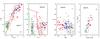 |
Fig. 8 Photometric diagrams for the stars in the DBS 78 region. Symbols as in Fig. 7. |
| In the text | |
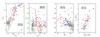 |
Fig. 9 Photometric diagrams for the stars in the DBS 102 region. Symbols as in Fig. 7. |
| In the text | |
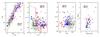 |
Fig. 10 Photometric diagrams for the stars in the DBS 160−161 region. Symbols as in Fig. 7. |
| In the text | |
|
Fig. 11 Distribution of stellar masses for the embedded clusters studied. Gray bars (light and dark) indicate more massive bins employed to compute the IMF slopes (Γ). Light gray bars and blue solid lines refer only to MS stars, whereas dark gray bars and black dashed lines refer to MS+PMS stars. |
| In the text | |
|
Fig. 12 Galactic rotation models applied at l = 301° to our Galaxy. The arrow indicates the adopted distance to the radial velocity of the radio sources according to the model. |
| In the text | |
|
Fig. 13 Galactic rotation models applied at l = 333° to our Galaxy. Arrows indicate the corresponding distance to the radial velocity of the radio sources according to the model. |
| In the text | |
|
Fig. 14 DBS 160−161: a) Mean Tb of the H I emission distribution associated with the B332.5−0.1−42 in the velocity range from −44.5 to −40.4 km s-1. Contour levels are from 80 to 110 K in steps of 5 K. Best-fitted ellipse to the bubble is indicated with dashed lines and the circle inside it indicates the ultra compact HII region GRS332.5−00.10. b) H I brightness temperature profile along |
| In the text | |
Current usage metrics show cumulative count of Article Views (full-text article views including HTML views, PDF and ePub downloads, according to the available data) and Abstracts Views on Vision4Press platform.
Data correspond to usage on the plateform after 2015. The current usage metrics is available 48-96 hours after online publication and is updated daily on week days.
Initial download of the metrics may take a while.