| Issue |
A&A
Volume 587, March 2016
|
|
|---|---|---|
| Article Number | A12 | |
| Number of page(s) | 16 | |
| Section | Stellar atmospheres | |
| DOI | https://doi.org/10.1051/0004-6361/201527614 | |
| Published online | 11 February 2016 | |
Near-infrared spectro-interferometry of Mira variables and comparisons to 1D dynamic model atmospheres and 3D convection simulations⋆
1
ESO, Karl-Schwarzschild-Str. 2,
85748
Garching bei München,
Germany
e-mail:
mwittkow@eso.org
2
Laboratoire Lagrange, UMR 7293, Université de Nice
Sophia-Antipolis, CNRS, Observatoire de la Côte d’Azur, BP 4229, 06304
Nice Cedex 4,
France
3
Department of Physics and Astronomy at Uppsala
University, Regementsvägen 1, Box
516, 75120
Uppsala,
Sweden
4
Zentrum für Astronomie der Universität Heidelberg (ZAH), Institut
für Theoretische Astrophysik, Albert-Ueberle-Str. 2, 69120
Heidelberg,
Germany
5
Sydney Institute for Astronomy, School of Physics, University of
Sydney, Sydney
NSW
2006,
Australia
6
South African Astronomical Observatory,
PO Box 9, 7935
Observatory, South
Africa
7
Astronomy, Cosmology and Gravity Centre, Astronomy Department,
University of Cape Town, 7701
Rondebosch, South
Africa
Received: 22 October 2015
Accepted: 23 December 2015
Aims. We aim at comparing spectro-interferometric observations of Mira variable asymptotic giant branch (AGB) stars with the latest 1D dynamic model atmospheres based on self-excited pulsation models (CODEX models) and with 3D dynamic model atmospheres including pulsation and convection (CO5BOLD models) to better understand the processes that extend the molecular atmosphere to radii where dust can form.
Methods. We obtained a total of 20 near-infrared K-band spectro-interferometric snapshot observations of the Mira variables o Cet, R Leo, R Aqr, X Hya, W Vel, and R Cnc with a spectral resolution of about 1500. We compared observed flux and visibility spectra with predictions by CODEX 1D dynamic model atmospheres and with azimuthally averaged intensities based on CO5BOLD 3D dynamic model atmospheres.
Results. Our visibility data confirm the presence of spatially extended molecular atmospheres located above the continuum radii with large-scale inhomogeneities or clumps that contribute a few percent of the total flux. The detailed structure of the inhomogeneities or clumps show a variability on time scales of 3 months and above. Both modeling attempts provided satisfactory fits to our data. In particular, they are both consistent with the observed decrease in the visibility function at molecular bands of water vapor and CO, indicating a spatially extended molecular atmosphere. Observational variability phases are mostly consistent with those of the best-fit CODEX models, except for near-maximum phases, where data are better described by near-minimum models. Rosseland angular diameters derived from the model fits are broadly consistent between those based on the 1D and the 3D models and with earlier observations. We derived fundamental parameters including absolute radii, effective temperatures, and luminosities for our sources.
Conclusions. Our results provide a first observational support for theoretical results that shocks induced by convection and pulsation in the 3D CO5BOLD models of AGB stars are roughly spherically expanding and of similar nature to those of self-excited pulsations in 1D CODEX models. Unlike for red supergiants, the pulsation- and shock-induced dynamics can levitate the molecular atmospheres of Mira variables to extensions that are consistent with observations.
Key words: techniques: interferometric / stars: AGB and post-AGB / stars: atmospheres / stars: fundamental parameters / stars: mass-loss
© ESO, 2016
1. Introduction
Mira variable stars are evolved low or intermediate mass stars located on the asymptotic giant branch (AGB) of the Hertzsprung-Russell (HR) diagram. They are long-period (~ 1 year) fundamental-mode (Wood et al. 1999) pulsators with V band amplitudes of typically 5–7 mag, near-IR K band amplitudes typically of 0.3–0.8 mag, and bolometric amplitudes typically of 0.5–1.2 mag, which correspond to luminosity variations by factors of about 1.5–3 (Whitelock et al. 2000).
AGB stars show mass-loss rates of (4 × 10⁻⁸−8 × 10⁻⁵)M⊙/yr (De Beck et al. 2010) and are one of the major sources of the chemical enrichment of galaxies and of dust in the universe. The AGB mass loss is thought to be driven by pulsation and convection, which levitate the atmospheres to regions where dust can form, and subsequently by radiation pressure on the dust grains dragging along the gas. Observationally, the presence of extended molecular atmospheres of Mira stars extending to a few stellar radii has been confirmed by spectro-interferometric observations (e.g., Mennesson et al. 2002; Perrin et al. 2004; Ohnaka et al. 2005; Wittkowski et al. 2008).
This scheme is theoretically constrained best for carbon-rich Mira stars, which are large amplitude pulsators where carbon has been dredged up to the surface so that carbon dust can form. Carbon dust has absorption coefficients that are high enough to drive the wind (e.g., Wachter et al. 2002; Mattsson et al. 2010). The process is less understood for oxygen-rich Mira stars, which typically have a lower mass and higher effective temperature than do the carbon-rich Miras. This is due to uncertainties regarding the properties of silicate grains in the close stellar vicinity and the resulting radiative pressure (Woitke 2006; Höfner 2008; Bladh & Höfner 2012). The dust condensation sequence is currently being refined, possibly including Al2O3 grains closest to the surface serving as seed particles, followed by relatively large scattering iron-free silicates at small radii, which can drive the wind, and – depending on the mass-loss rate – subsequently by iron-coated silicates at larger radii (e.g., Karovicova et al. 2013; Bladh et al. 2015).
For semi-regular AGB stars with lower pulsation amplitudes as well as for red supergiants, it is not yet clear how the atmospheres are levitated to regions that are favorable to dust formation and growth. Indeed, Arroyo-Torres et al. (2015) show that current 1D pulsation models of red supergiants did not lead to shock fronts that enter the inner atmospheres of red supergiants1. For 3D convection models of red supergiants, there were shocks in the atmospheres, mostly on smaller (i.e. granular), but not on global scales. However, while travelling outward, the density behind the shocks declined drastically so that not enough material was lifted to cause noticeable optical depths significantly outside one stellar (photospheric) radius. Both 1D and 3D model attempts cannot currently levitate the atmospheres to observed extensions of a few stellar radii where dust can form. This suggests a missing process for levitating the atmospheres of red supergiants.
Unlike for red supergiants, however, recent 1D dynamic model atmospheres based on self-excited pulsation models of oxygen-rich Mira stars (CODEX models) (Ireland et al. 2008, 2011; Scholz et al. 2014) were successful at describing interferometric observations of these sources, including their extended atmospheric molecular layers (Woodruff et al. 2009; Wittkowski et al. 2011; Hillen et al. 2012). However, they do not yet include a wind. Observations indicate surface inhomogeneities of the extended molecular layers corresponding to a few spots across the stellar surface at intensity levels of a few percent (e.g., Wittkowski et al. 2011; Haubois et al. 2015).
Freytag & Höfner (2008) have presented 3D radiation hydrodynamic (RHD) simulations of the convective interior and the atmosphere of a typical AGB star. They find that the surface of the model star is dominated by a few giant convection cells. The interaction of irregular pulsations with the convective cells triggers shock waves in the photospheric layers. These shock waves were found to be roughly spherically expanding, similar to those of 1D pulsation models, but with certain non-radial structures. They show that these shock waves levitate the material into regions where dust can form. However, these predictions of 3D CO5BOLD dynamic models of AGB stars have so far not been compared with spatially resolved observations of the extended atmospheres of AGB stars. The model has been compared to data of a red supergiant, VX Sgr, by Chiavassa et al. (2010), where it surprisingly provided a better fit to the data than similar models of red supergiants (see also the discussion of VX Sgr in Arroyo-Torres et al. (2015).
Here, we analyze the spectro-interferometric data of the Mira variables R Cnc, X Hya, and W Vel again from Wittkowski et al. (2011), together with so far unpublished second epochs of these targets with a separation of three months. We also analyze new spectro-interferometric data of the Mira variables o Cet, R Aqr, and R Leo in the same way. For the first time we compare spectro-interferometric observations of Mira stars to predictions by these 3D CO5BOLD dynamic model atmospheres of AGB stars (Freytag & Höfner 2008), in addition to those by 1D CODEX dynamic model atmospheres (Ireland et al. 2008, 2011; Scholz et al. 2014).
2. Observations and data reduction
Observation log.
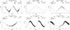 |
Fig. 1 Visual lightcurves of our sources as a function of Julian Date (top axis) and variability phase (bottom axis) around the dates of observation. The solid line denotes a sinusoidal fit to the data (crosses) obtained from the AAVSO and the AFOEV databases. The vertical dashed lines indicate the epochs of our observations. |
We obtained a total of 20 spectro-interferometric snapshot observations of the Mira variables R Cnc, W Vel, X Hya, R Aqr, o Cet, and R Leo with the AMBER instrument (Petrov et al. 2007) in the K-band medium resolution modes (MR-K 2.1 μm, MR-K 2.3 μm, R ~ 1500), employing external FINITO fringe tracking. Table 1 shows the details of our observations, including the dates, the baselines, the modes, and the calibrators used. Figure 1 shows the visual lightcurves of our sources as obtained from the AAVSO and AFOEV databases around the dates of our observations. R Cnc was observed at three epochs; W Vel, X Hya, and o Cet at two epochs each; and R Aqr and R Leo at one epoch each. Observations of these targets were interleaved with observations of interferometric calibrators. Calibrators were selected with the ESO Calvin tool, and their angular K-band diameters were adopted from Lafrasse et al. (2010) (81 Gem: 2.93 mas ± 0.03 mas; ι Hya: 3.58 mas ± 0.28 mas; 31 Ori: 4.02 mas ± 0.39 mas; 31 Leo: 3.33 mas ± 0.34 mas; γ Pyx: 3.00 mas ± 0.27 mas; φ Aqr: 6.16 mas ± 0.50 mas; β Cnc: 5.21 mas ± 0.36 mas). For α Cet, we instead adopted the measured K-band angular diameter of 11.05 mas ± 0.55 mas from Wittkowski et al. (2006). The first epochs of R Cnc, X Hya, and W Vel were previously analyzed and published by Wittkowski et al. (2011). Here, we reduced and analyzed the complete data set in a uniform way with the aims of studying the visibility variability and comparing the observations not only to 1D CODEX dynamic model atmospheres based on self-excited pulsation models, but also for the first time to 3D CO5BOLD dynamic model atmospheres including pulsation and convection.
Each data set of Table 1 typically consists of a calibrator observation taken before the science target observation, the science target observation, and another calibrator observation taken afterward. Each of these observations typically consist of five files of 170 scans each, accompanied by a dark and a sky file. It is essential for a good calibration of the interferometric transfer function that the performance of the FINITO fringe tracking is comparable between corresponding calibrator and science target observations. To this purpose, we inspected the FINITO lock ratios and the FINITO phase rms values as reported in the fits headers of each file. In a few cases we deselected individual files for which these values deviated by more than about 20%. In rare cases we had to discard a complete data set because the FINITO phase rms values were systematically very different by clearly more than about 20% between science target observation and calibrator observations. This concerned one additional data set of R Cnc and one additional data set of X Hya obtained in MR21 mode on 2008 December 30, as well as data of o Cet obtained in MR23 mode on 2011 September 30.
We obtained averaged visibility and closure phase values from the raw data using the latest version, version 3.0.8, of the amdlib data reduction package (Tatulli et al. 2007; Chelli et al. 2009). The absolute wavelength calibration and the calibration of the interferometric transfer function were performed using IDL scripts developed in house. For the absolute wavelength calibration, we correlated the AMBER flux spectra with a reference spectrum that included the AMBER transmission curve, the telluric spectrum estimated with ATRAN (Lord 1992), and the expected stellar spectrum using the spectrum of the K giant BS 4432 from Lançon & Wood (2000). For calibrating the interferometric transfer function, we used an average transfer function of the calibrator observations obtained before and after that of the science target. In some cases, when this sequence was not available, we used the two closest calibrators in time. The error of the transfer function was estimated by the difference between the two calibrator measurements. The error of the final visibility spectra includes the statistical noise of the raw data and the systematic error of the transfer function.
All obtained flux, squared visibility, and closure phase data are shown below in Figs. A.1−A.6, together with model predictions as outlined in Sect. 4. These figures include one row of flux, squared visibility, and closure phase panels for each row of Table 1, so they show the results of each dataset individually. The middle panels showing the squared visibility data include three lines corresponding to the three baselines of each AMBER dataset, where the shortest baseline corresponds to the highest visibility curve and the longest baseline to the lowest visibility curve.
SAAO photometry.
We also obtained concurrent near-infrared JHKL photometry of R Cnc, X Hya, and W Vel at the South African Astronomical Observatory (SAAO) Mk II instrument. Table 2 lists the obtained photometry and the estimated bolometric magnitudes using the procedures outlined by Whitelock et al. (2008). We used AV values from Whitelock et al. (2000). For o Cet, R, Leo, and R Aqr, we estimated bolometric magnitudes at the phases of our observations based on the mean mbol values and the amplitudes Δmbol from Whitelock et al. (2000) (o Cet: mbol 0.56 and Δmbol 1.01; R Leo: mbol 0.65 and Δmbol 0.63; R Aqr: mbol 2.23 and Δmbol 0.91). We estimated mbol = 1.04 for o Cet at phase 0.1, mbol = 0.75 for R Leo at phase 0.6, and mbol = 2.37 for R Aqr at phase 0.6. We adopted errors of 0.05 mag for the concurrent measurements of R Cnc, X Hya, and W Vel, and 0.1 mag for the estimates for o Cet, R Leo, and R Aqr.
3. Visibility results and variability
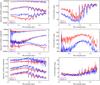 |
Fig. 2 Direct comparison of (left) the visibility function and (right) the closure phases of data obtained of the same source at virtually the same baseline length and angle but at different epochs. From top to bottom: data sets 1&6 of R Cnc, 2&4 of R Cnc, 9&11 of X Hya, cf. Table 1. Errors of the squared visibility amplitudes are in the range of 5–15%; errors of the closure phases are in the range of 5–15 deg. |
The AMBER medium spectral resolution visibility results shown in Figs. A.1–A.6 exhibit the same characteristic shape as a function of wavelength as previously observed by Wittkowski et al. (2011). The squared visibility amplitudes within the K-band show a maximum near 2.25 μm and decrease both toward shorter and longer wavelengths with pronounced drops at the positions of the CO bandheads. This is interpreted as an indication of extended atmospheric molecular layers of – most importantly – H2O (centered at ~2.0 μm) and CO (longward of 2.29 μm). The closure phases as a function of wavelength show a characteristic shape as well, where deviations from point symmetry are observed at all wavelengths, depending on how well the target is resolved, with most pronounced deviations from symmetry at the positions of H2O and CO bands. Wittkowski et al. (2011) interpreted this closure phase signal as a signature of large-scale inhomogeneities or clumps in the extended molecular layers contributing a few percent of the total flux. This is consistent with imaging studies of the Mira star X Hya by Haubois et al. (2015). Their reconstructed images at two epochs separated by about two months also revealed a variability of the asymmetric structures.
Our data sets of R Cnc and X Hya include data obtained at different epochs using the same mode with virtually the same projected baseline lengths, so that we can attempt to directly (i.e. model independently) probe for visibility variability. In particular, data set numbers 1 and 6 of R Cnc taken in mode MR23, data set numbers 2 and 4 of R Cnc taken in mode MR21, and data set numbers 9 and 11 of X Hya were taken with projected baseline lengths that differ by only 0.1% (cf. Table 1) and projected baseline angles that differ by only 1–3 deg. Figure 2 shows a comparison of the visibility and closure phase data for these three pairs. The visibility data of R Cnc at the short and intermediate baseline differ within the error bars, so that we cannot conclude on a variation in the overall angular diameter of the star within a phase difference of 0.2. However, the visibility on the longest baselines and the closure phases do show significant changes within a phase difference 0.2. Both the low visibilities on the third baseline, which fully resolves the stellar disk, and the closure phases are affected by the inhomogeneities or clumps mentioned above. This indicates a variability in the detailed structure of these clumps for phase differences as small as 0.2 (cf. data sets nos. 2 and 4), again consistent with the imaging study by Haubois et al. (2015). Hereby, data sets nos. 1 and 6 were taken during consecutive cycles, so that for this comparison we cannot distinguish between intracycle and cycle-to-cycle variabilities. For the comparison of the two datasets of X Hya, we cannot conclude on any variability within two months, owing to the lower spatial resolution that we obtained for this star.
4. Comparison to model atmosphere predictions
Fit results.
As a first approach to characterizing the angular size of the targets, we fit a uniform disk (UD) model to the squared visibility amplitudes obtained at a near-continuum wavelength band between 2.22 μm and 2.28 μm. Previous studies have shown that this wavelength band is not contaminated much by molecular bands and that it provides a good estimate of the angular diameter of continuum-forming layers. We merged data of the same targets that were obtained at the same epoch with separations of up to a few days. Our previous studies (Wittkowski et al. 2011) indicated surface inhomogeneities at flux levels of a few percent that affected low visibility values, while higher visibility values within the first lobe were not affected by inhomogeneities and were consistent with spherically symmetric models. We thus excluded squared visibility amplitudes below 0.01 in our fitting procedure, and these correspond to flux levels below 10%. The resulting UD angular diameters  obtained at a wavelength of 2.25 μm, together with the corresponding reduced
  values are listed in Table 3, together with the fit results of the 1D and 3D model atmospheres described below. Reduced values are partly above unity. The most likely cause of the comparably higher values is that we underestimated the systematic error of the interferometric transfer function. Our error was estimated by the variability of the transfer functions obtained before and after the science target observations. There may be systematic effects between the transfer function of (almost) unresolved calibrator stars and (often fully resolved) science targets that could not be included in this error, even though we made sure that the FINITO fringe-tracking performance (phase rms values) was similar (cf. Sect. 2). We note that the statistical error based on the individual scans and that of the uncertainty of the adopted calibration star diameters are smaller than for the transfer function stability.
We obtained values for R Cnc between 13.1 mas and 13.3 mas at phases between 0.3 and 0.5, for W Vel of 7.4 mas at phases between 0.9 and 1.1, for X Hya between 6.2 mas and 5.7 mas at phases between 0.7 and 0.9, for R Aqr of 18.4 mas at phase 0.6, for o Cet between 28.6 mas and 28.3 mas at phase 0.1, and for R Leo of 29.6 mas at phase 0.6. Errors range between 1% and 3%. For those targets for which we obtained data at different phases (R Cnc, W Vel, X Hya) separated by 0.2, there are no significant differences of . These values are broadly consistent with earlier estimates of the angular diameters of these targets. For example, Mennesson et al. (2002) obtained broad-band K angular diameters of 16.9 ± 0.6 mas for R Aqr at phase 0.4, for o Cet between 24.4 ± 0.1 mas and 28.8 ± 0.1 mas at phases 0.9–0.0, and for R Leo between 28.2 ± 0.1 mas and 30.7 ± 0.1 mas at phases between 0.2 and 0.3. Woodruff et al. (2004) estimated a Rosseland angular diameter of o Cet between 28.9 ± 0.3 mas and 34.9 ± 0.4 mas at phases of 0.1 and 0.4, respectively. Fedele et al. (2005) estimated a Rosseland angular diameter of R Leo between 28.5 ± 0.4 mas and 26.2 ± 0.8 mas at phases of 0.1 and 0.0, respectively.
The visibility curves of Figs. A.1–A.6 show that the UD curves provide good fits to the measured visibilities in the near-continuum bandpass around 2.25 μm at the different baselines. The measured visibilities drop significantly below the UD curves toward shorter and larger wavelengths, which are affected by molecular bands of H2O and CO. This behavior is consistent with our earlier results (Wittkowski et al. 2011) and has been interpreted as an indication that extended molecular layers are located above the continuum-forming layers.
Closure phases are wavelength-dependent resembling the locations of the water vapor band around 2.0 μm and the CO band and bandheads longward of 2.29 μm. As in Wittkowski et al. (2011) we interpret the closure phase signal as an indication of a few surface spots across the extended molecular atmosphere. As spherical model atmospheres (cf. Sect. 4.1) are generally consistent with squared visibility amplitudes above ~ 0.01, and deviations occur at lower values, we can estimate that these inhomogeneities contribute up to ~10% of the total flux.
4.1. Comparison to 1D CODEX model atmospheres
As a next step, we compared our data to 1D CODEX model atmospheres of Mira variables by Ireland et al. (2008, 2011) as in Wittkowski et al. (2011). These model atmospheres are based on self-excited pulsation models and use the opacity sampling method to calculate model intensity profiles. CODEX models are available in four different series that correspond to different stellar parameters of the underlying hypothetical non-pulsating parent star. The parameters of the CODEX model series are listed in Table 4.
Parameters of the CODEX model series.
The parameters of the o54 series are designed to match those of the Mira variable o Cet, those of the R52 series to match the Mira variable R Leo, and those of the C50/C81 series to match a typical longer-period Mira star such as R Cas. C81 is a higher luminosity series compared to C50. Each series consists of a number of models that correspond to different phases with a separation of ~0.1 and covering a few cycles. The o54 series deliberately includes cycles where the atmosphere is particularly compact and particularly extended, in addition to normal cycles. The CODEX models contain a simple description of dust, which only moderately affects the equation of state, the spectrum, and the effective temperature and which does not lead to a wind (Ireland et al. 2008, 2011). We note that the nature of real dust in Miras is still rather controversial regarding the layers, the composition, and the grain sizes (e.g., Bladh & Höfner 2012; Goumans & Bromley 2012; Gail et al. 2013; Karovicova et al. 2013; Bladh et al. 2015; Gobrecht et al. 2016).
We tabulated the CODEX intensity profiles in steps of 0.0005 μm (λ/ Δλ = 40 000 at λ = 2 μm) for wavelengths between 1.4 μm and 2.5 μm, covering the AMBER medium resolution modes at a sufficient spectral resolution to average more than 20 monochromatic intensity profiles for each individual AMBER spectral channel. Synthetic visibility values were computed using the Hankel transform and averaging monochromatic squared visibility amplitudes over the AMBER spectral channels.
We fit the visibility data of each of our targets and epochs separately to every available CODEX model, where the Rosseland angular diameter θRoss was the only free parameter, and we selected the models with the best reduced values. The Rosseland angular diameter is the diameter that corresponds to the model layer where the Rosseland optical depth equals unity (τRoss = 1)2. We then selected a series that provided good fits to all epochs of a given target and used the best-fit model of only this series. For o Cet and R Leo, we restricted the fits to the o54 and R52 series, respectively, which are designed to match the parameters of these sources. As for the UD fits, we excluded squared visibility values below 0.01, which correspond to flux levels below 10% because these may be affected by surface inhomogeneities. The error of θRoss is dominated by the choice of the model, reflecting the uncertainty of defining a radius of a star with a very extended atmosphere. We used the standard deviation of the θRoss values based on the ten best-fit models of the adopted series as the error of θRoss.
Parameters of the 3D model st28gm06n06.
The resulting best-fit models, together with their model phase, effective temperature, luminosity, and the corresponding θRoss and values are listed in the middle panel of Table 3 for each of our sources and epochs. The model phases of the best-fit CODEX models are generally consistent with the visual phases within 0.1–0.2, which is considered the uncertainty of phase assignments (Ireland et al. 2011). Exceptions are the near-maximum observation of W Vel at phase 0.1, of X Hya at phase 0.9, and of o Cet at phase 0.1, for which the molecular features can be better described by near-minimum models. Discrepancies between observed and model phases in particular for near-maximum observations has already been noted by Hillen et al. (2012). This might be caused by an absence of a wind in the CODEX models. Bladh et al. (2015) show that models with and without a wind have different colors because molecular features are related to the structure in the wind acceleration region.
The Rosseland angular diameters are broadly consistent (within 1–3σ) with the and with previous observations listed above. This is a satisfactory agreement, considering that the UD model is not expected to be a very good model even for the near-continuum bandpass, that the estimate of the Rosseland angular diameter is model-dependent, and that in general a radius definition of a star with a very extended atmosphere is problematic (cf. Scholz 2001). As for the values, the θRoss values also do not indicate an intracycle or cycle-to-cycle variability within the limited separations (~2 months, corresponding to phase differences of ~0.2) and within our uncertainties.
Figures A.1 to A.6 show the synthetic flux, squared visibility amplitudes, and closure phases as predicted by the best-fit CODEX models compared to the observed quantities. The flux spectra predicted by the CODEX model are consistent with our observed AMBER spectra within the error bars. The observed spectra taken with the AMBER MR-K 2.3 μm mode are systematically higher than the model-predicted spectra in the wavelength range between about 2.1 μm and 2.2 μm. However, the same wavelength range is consistent for data taken with the AMBER MR-K 2.1 μm mode. This discrepancy is thus most likely to be caused by a systematic calibration effect of the AMBER MR-K 2.3 μm mode. Although some spectral calibration can be performed, we note that the AMBER instrument is optimized for interferometry and that it is not a good spectrograph with its single-mode fibers.
The synthetic visibility curves as predicted by the best-fit CODEX models are consistent with the measured visibility curves. In particular, they match the decrease in the visibility function well at the location of the H2O band around 2.0 μm and at the location of the CO bandheads longward of 2.29 μm. This shows that the CODEX models predict an extended molecular atmosphere and that the model-predicted extensions of the atmosphere are consistent with our observations. Deviations between observed and model-predicted visibility amplitudes below ~0.1 and the wavelength-dependent closure phases showing strongest deviations from point symmetry at the locations of the water vapor and CO bands indicate a few inhomogeneities within the molecular atmosphere within an overall spherical geometry. This is consistent with similar results for oxygen-rich Mira variables by, for example, Le Bouquin et al. (2009), Wittkowski et al. (2011), Monnier et al. (2014), and Haubois et al. (2015).
4.2. Comparison to 3D CO5BOLD model atmospheres
As a next step we compared our visibility data to predictions by 3D CO5BOLD dynamic model atmospheres including pulsation and convection of an AGB star by Freytag & Höfner (2008), which represents the first direct comparison of interferometric data of an AGB star to this model. Freytag & Höfner (2008) used the RHD code CO5BOLD (Freytag et al. 2012) to produce time-dependent 3D models of the outer convective layers and the atmosphere of an AGB star. In short, the stellar parameters were chosen to closely resemble those of a 1D model studied by Höfner et al. (2003). The 3D simulations started with a hydrostatic, spherically symmetric structure, mapped onto a 3D grid.
Small-amplitude random velocities were added. In a sequence of models, the physical parameters of the dynamical model and the size of the computational box were adjusted until the flow properties stabilized. Dust formation was added as a last step without feeding the dust opacities back into the RHD equations. Models use gray (Rosseland) opacities, computed from detailed continuum and line opacities from atoms and molecules. In fact, the opacities are merged from Rosseland opacity tables from PHOENIX and the OPAL project for the atmosphere and the interior, respectively. Here, we used their final 3D model st28gm06n06. The basic parameters of this model are listed in Table 5. Compared to the CODEX series, this is an AGB star model with relatively high luminosity, relatively large radius, and relatively low effective temperature. Indeed, the initial 1D model from Höfner et al. (2003) was designed to match a C-rich AGB star, but a O-rich atmosphere was used for the 3D modeling. Unlike the CODEX models, which include a simple description of dust, the 3D model is dust-free. Thus far this is the only 3D dynamic model atmosphere of an AGB star that is currently readily available. New AGB models, including gray models with the current version of CO5BOLD and a much better resolution, as well as first non-gray models, are being prepared (cf. Freytag 2015) and may become available within the next years.
We used the pure-LTE radiative transfer Optim3D (Chiavassa et al. 2009) to compute intensity maps from 12 snapshots of the RHD simulation st28gm06n06. These snapshots cover about 8.5 months with separations of about 0.7 months and thus cover varying stellar parameters (luminosities between 5418 L⊙ and 8170 L⊙, radii between 489 R⊙ and 519 R⊙, and effective temperatures between 2190 K and 2469 K). Optim3D takes the Doppler shifts occurring due to convective motions into account. The radiative transfer equation is solved monochromatically using pretabulated extinction coefficients as a function of temperature, density, and wavelength. The lookup tables are computed using the same extensive atomic and molecular continuum and line opacity data as the latest generation of MARCS models (Gustafsson et al. 2008). Again, a description of dust has not been added. We computed intensity maps in the wavelength range from 1.90 μm to 2.60 μm with a constant spectral resolution of about 20 000. Moreover, for every wavelength, a top-hat filter including five wavelengths close by has been considered. In total, about 70 000 images for every simulation snapshot were computed to cover the wavelength range of our AMBER observations with a spectral simulation so that we can average more than ten wavelengths for each AMBER spectral channel in a similar manner to what was performed for the CODEX models in Sect. 4.1 above.
Instead of a direct comparison to the intensity maps, we chose to compare our data to azimuthally averaged intensity profiles obtained from the intensity maps for a number of reasons: (1) The detailed surface structure has a random origin and is unlikely to match the observations at a given epoch exactly. (2) Freytag & Höfner (2008) discuss that the convection cells in the 3D simulations are so large that the associated shock fronts appear almost spherical and that they are consistent with pulsating1D models. (3) Our interferometric data already indicated that the visibilities above about a flux level of 10% are consistent with spherically symmetric models (see Sect. 4.1). (4) We intend to compare our data to the results from the 3D model atmospheres in the same way as for the 1D CODEX models and to compare the intensity profiles of these modeling attempts.
We obtained the azimuthally averaged intensity profiles using the method explained in detail by Chiavassa et al. (2009). They were constructed using rings that are regularly spaced in μ (where μ = cos(θ) with θ being the angle between the line of sight and the radial direction). Finally, we estimated synthetic squared visibility amplitudes from the azimuthally averaged intensity profiles using the Hankel transform and averaging over the bandpass of each AMBER spectral channel as we did for the CODEX models. These procedures follow those described by Arroyo-Torres et al. (2015) for RHD simulations of red supergiants.
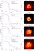 |
Fig. 3 Left panels: intensity profiles of (blue) the 1D CODEX model o54/286100 compared to (red) the azimuthally averages intensity profiles of snapshot 68 of the RHD simulation st28gm06n06 at bandpasses (from top to bottom) 2.00 μm–2.01 μm (water vapor), 2.25 μm–2.26 μm (continuum), 2.2934 μm–2.2936 μm (CO 2−1), and 2.47 μm–2.48 μm (CO). Both models provide a satisfactory fit to our visibility data of o Cet obtained in October 2012. The purple dashed line indicates a UD as reference. The intensities are normalized so that the integrated flux of each curve is unity. Right panels: images of the 3D intensity maps of snapshot 68 at the same bandpasses. A squareroot color scale is used to enhance the low intensities of the extended molecular atmosphere. |
In the same way as for the CODEX models in Sect. 4.1 we fit our visibility data of each target and epoch to each of the available 12 snapshots of the RHD simulation and chose the snapshot with the best value. The fit results including the best-fit radius and the corresponding value are listed in the righthand panel of Table 3, together with the effective temperature and luminosity of the best-fit snapshot. Here, the radius corresponds to the model radius, which is calculated from the luminosity and effective temperature of the snapshot. A layer corresponding to a Rosseland optical depth of unity as used for the CODEX models is more difficult to define for a 3D model with a different model structure in different directions. However, the radius defined in this way should be comparable to the Rosseland radius used with the CODEX models.
The synthetic flux and squared visibility spectra of the best-fit RHD snapshot are shown again in Figs. A.1–A.6 compared to the observed data and to the predictions by the best-fit CODEX models.
The flux spectra of the RHD simulation have a systematically different shape than the observations and are compared to the CODEX flux spectra, in particular in the wavelength range shortward of the near-continuum bandpass at ~2.25 μm down to about 2.0 μm, a range that is dominated by water vapor bands. The reason for this difference is not yet known.
The synthetic squared visibility amplitudes based on the RHD simulation are consistent with our measurements and with the predictions by the CODEX models. They predict the decrease in the visibility function at the locations of the water vapor band centered at about 2.0 μm and at the locations of the CO bandheads as well as the CODEX models. This means that the 3D CO5BOLD dynamic model atmospheres also lead to an extended molecular atmosphere that is consistent with observations. Likewise, the best-fit angular diameters and the values between the fits to the CODEX models and to the RHD simulation are comparable, considering the caveats already mentioned in Sect. 4.1 and considering that the stellar parameters of the RHD simulation do not match those of our sources well.
In Fig. 3 we compare the model predicted intensity profiles at certain bandpasses for the example of the 1D CODEX model o54/286100 and the 3D model snapshot 68, which both provide a good fit to our visibility data of o Cet obtained in October 2012. We chose four bandpasses, including a water vapor band at 2.0 μm, a near-continuum band at 2.25 μm, a band centered on the CO 2−0 line at 2.2935 μm, and a band including CO and possibly water vapor toward the edge of the K-band at 2.47 μm. We also show 2D images of the intensity distribution based on the 3D model. These images use a squareroot color scale to visually enhance the low intensities of the extended molecular layers. Both model attempts predict a compact peak intensity up to about 1 R∗ and an extended envelope up to about 2 R∗. The peaks in the azimuthal average of the 3D models at about two stellar radii are a signature of density peaks at the position of shock fronts. These peaks do not significantly affect our results. The ratio of the extended component relative to the central compact component varies as a function of wavelength. In other words, our visibility variation as a function of wavelength more precisely indicates different flux contributions of the extended atmosphere rather than different spatial extensions. The exact intensity profiles of the two modeling attempts differ, but they agree in the overall spatial extent of the extended component and in the wavelength-dependent flux contributions of the extended component. High-fidelity interferometric imaging campaigns at high spectral resolution are needed to constrain the exact shape of the intensity profiles as a function of wavelength and to differentiate further between different model atmospheres of AGB stars. The images of the 3D model atmosphere indicate an inhomogeneous distribution of the extended molecular layers, which in this example are more elongated toward the south than toward the north. This is qualitatively consistent with the observed inhomogeneities or clumps discussed above and by Wittkowski et al. (2011) and Haubois et al. (2015) based on AMBER data. In this context, we also note that for R Cnc, W Vel, and X Hya, all our current observations are taken along similar position angles, thus providing limited information on the global geometry of the photospheres of these objects, while observations of R Aqr, o Cet, and R Leo cover a wider range of position angles.
4.3. Comparison of the broad-band photometry to model atmosphere predictions
Observed and model-predicted colors.
We collected simultaneous JHKL broad-band photometry at the SAAO for two epochs of three of our six targets as described in Sect. 2 and as listed in Table 2. The primary goal of these observations was to obtain simultaneous bolometric fluxes and other fundamental stellar parameters (Sect. 5). Here, we compare the broad-band photometry to synthetic values predicted by the model atmospheres to constrain them further. For each of these targets and epochs, Table 6 shows the observed J − H, J − K, and J − L colors derived from Table 2 taking the extinction as listed there into account, together with the synthetic values from the best-fit CODEX model and the best-fit 3D snapshot (cf. Table 3). To calculate the synthetic values, we used the H,K,L filter curves from Glass (1973) and the J filter curve from Glass (1993). The predicted J − H, J − K, and J − L broad-band colors of the best-fit CODEX models generally agree with the observations to about 0.0–0.3 mag. The predictions of the best-fit 3D snapshots in general agree similarly well for the J − H and J − K colors, while they predict much bluer J − L colors near 0 mag. The latter discrepancy can most likely be explained because the 3D models do not include any dust description while the CODEX models do include a simple description of dust (cf. Sects. 4.1 and 4.2). Indeed, using the dust-free predecessors of the CODEX models, the P/M model series by Ireland et al. (2004b,a), we also obtain typical J − L colors near 0 mag (for example, model P20 gives J − H = 0.41, J − K = 0.28, J − L = 0.03). This means that dust is transparent for our sources at J, H, and K bands and starts to contribute to broad-band colors from the L-band onward. Hereby, the simple dust description of the CODEX models is sufficient to explain the broad-band J − L color. These findings are consistent with dust grains being transparent at near-infrared wavelengths as discussed by Ireland et al. (2005), Norris et al. (2012), and Bladh et al. (2015).
5. Fundamental stellar parameters
Fundamental stellar parameters.
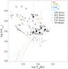 |
Fig. 4 Location of our sources in the HR diagram as listed in Table 7, together with those of the CODEX models and the 3D model st28gm06n06. Shown are the positions of individual CODEX models with different symbols for each of the four series, where the orange symbols represent the locations of the hypothetical non-pulsating parent star. The orange symbol and error bars of the 3D model denote the average and standard deviation of different snapshots of the 3D model. Individual snapshots of the 3D model are not shown. Also shown are stellar evolutionary tracks of the early AGB from Lagarde et al. (2012) for 1.0, 1.25, 1.5, and 2.0 solar masses and solar chemical composition. |
We used the UD diameters at a near-continuum wavelength of 2.25 μm from Table 3 as a model-independent estimate of the stellar angular continuum radius. These are generally consistent with model-dependent Rosseland angular diameters (cf. the discussion above in Sect. 4). Together with apparent bolometric magnitudes based on SAAO photometry (Sect. 2) and with distance estimates from the literature, we computed linear radii, effective temperatures, and luminosities of our sources at the respective phase. The resulting values are listed in Table 7. R Aqr has a recent high-precision VLBI parallax measurement (Min et al. 2014), which we used. For our other sources, we used the period-luminosity (P − L) distances from Whitelock et al. (2008). It is difficult to give a precise error on the P − L distance making us conservatively adopt an error of 15%.
Compared to the best-fit CODEX models, the measured Teff values are typically lower than those of the CODEX models. The luminosities of the best-fit CODEX models are generally consistent with the observed luminosities within the error bars, but tend to be systematically higher within the uncertainty. Compared to the best-fit 3D snapshots, the measured Teff values are higher than those of the models except for R Cnc. The luminosities of the 3D snapshots tend to be higher than the measured values, although they are consistent within the errors for R Cnc, W Vel, and X Hya. However, we note that, similar to the discussion of the radius in Sect. 4.1, it is also difficult to define an effective temperature for a star with a very extended atmosphere. The definition of the effective temperature depends on the model-dependent definition of the stellar radius.
Figure 4 illustrates the positions of our sources in the HR diagram compared to the positions of the individual CODEX models and the average of the 3D CO5BOLD model. Also shown are the stellar evolutionary tracks of the early AGB by Lagarde et al. (2012) for masses between 1.0 M⊙ and 2.0 M⊙ and solar chemical composition. The observed positions are consistent with the ranges of the model atmospheres and are located shortly above the early AGB evolution.
6. Summary, discussion, conclusions
We obtained AMBER near-infrared K-band (1.9–2.5 μm) spectro-interferometric (spectral resolution R ~ 1500) observations of a total of six Mira variable AGB stars. For three of the sources, observations were obtained at two epochs separated by about two months using virtually the same projected baseline lengths and angles.
The squared visibility amplitudes as a function of wavelength within the K-band show a maximum near 2.25 μm and decrease both toward shorter and longer wavelengths with pronounced drops at the positions of the CO bandheads. This is interpreted as an indication of extended atmospheric molecular layers of – most importantly – H2O (centered at ~2.0 μm) and CO (longward of 2.29 μm) as previously observed for Mira stars with AMBER by Wittkowski et al. (2008, 2011), Haubois et al. (2015). The closure phases as a function of wavelength show a characteristic shape as well, where deviations from point symmetry are observed at all wavelengths, depending on how well the target is resolved, with most pronounced deviations from symmetry at the positions of H2O and CO bands. This closure-phase signal is interpreted as a signature of large-scale inhomogeneities or clumps at the photospheric layers and within the extended molecular layers. These inhomogeneities or clumps contribute a few percent of the total flux. Observations taken at two epochs separated by about two months indicate a variability of the detailed structure of the inhomogeneities, while a variability of the overall radius could not be detected within our calibration uncertainties.
We compared our data with the latest 1D dynamic model atmospheres based on self-excited pulsation models (CODEX models) and for the first time also with 3D radiation hydrodynamic (RHD) simulations of the convective interiors and the atmospheres of AGB stars (CO5BOLD code). For the latter we chose to use azimuthally averaged intensity profiles because our main interest in this current investigation concerns the overall extension of the atmospheres and because we aim at comparing the 3D models to the results by 1D models. In addition, we have previously shown that visibilities above a flux level of about 10% are consistent with spherically symmetric models so that the detailed 3D structure mainly concerns only relatively low flux levels. Both model attempts provide satisfactory fits to our data and, in particular reproduce the wavelength dependence of the visibility data. This means that both models include a spatially extended molecular atmosphere that is consistent with our observations. A comparison between the intensity profiles of the best-fit 1D and 3D models show that indeed both model attempts include an extended atmosphere up to roughly two to three stellar radii and that the wavelength-dependent flux contributions of the extension are consistent with observations. This agreement of both the different 1D and 3D modeling attempts with our data supports the theoretical result by Freytag & Höfner (2008) that shocks induced by convection and pulsation in 3D models are roughly spherically expanding and of similar nature to those of 1D self-excited pulsations.
Moreover, our results show that indeed both modeling attempts, 1D pulsation models and 3D convection simulations, can levitate the atmosphere of Mira stars to at least two to three stellar radii, which is consistent with our observations. We note that, on the contrary the same modeling attempts failed to extend the atmospheres of red supergiant stars to similarly observed extensions (Arroyo-Torres et al. 2015).
In addition, observed and model-predicted broad-band J − H and J − K are consistent for both the 1D CODEX and 3D CO5BOLD models, while the J − L color can only be re-produced by the 1D CODEX, which includes a simple dust description, and not by the dust-free 3D CO5BOLD models, indicating that dust starts to contribute to broad-band colors from the L-band onward.
The detailed intensity profile across the stellar disk could not be constrained by our current snapshot observations. This would require future imaging campaigns. More detailed comparisons between 1D and 3D models and between observations and 3D models along different angles are planned for a forthcoming publication. However, devising a proper strategy for comparing variable objects with dynamical models and, in particular, 3D models is a non-trivial task. For more detailed comparisons, one should try to disentangle (or at least discuss) whether discrepancies are due to bugs in the code, the omission of essential physics (such as dust, magnetic fields, rotation), simplifications (such as gray opacities, finite numerical grid), or inappropriate stellar parameters. Moreover, for a dynamic and non-spherical structure, it is a fundamental problem to select the correct snapshot in time and the correct viewing angle.
Based on the model-independent UD diameters at a near-continuum bandpass around 2.25 μm, on SAAO photometry to estimate the bolometric flux, and on distances available in the literature, we estimated absolute radii, effective temperatures, and luminosities of our sources at the respective variability phases. The UD diameters at 2.25 μm are generally consistent with Rosseland angular diameters that are derived from the comparison with model atmospheres. In general, the CODEX models tend to have higher effective temperatures than observed. The 3D RHD simulation tends to have lower effective temperatures and higher luminosities than observed for our sample. Observational variability phases are mostly consistent with those of the best-fit CODEX models, except for near-maximum phases, where data are better described by near-minimum models. The availability of more complete model grids of different stellar parameters would be important for better matching observed stellar parameters.
Acknowledgments
This paper uses observations made at the South African Astronomical Observatory (SAAO). We are grateful to Francois van Wyk for doing the infrared photometry from SAAO. PAW thanks the South African National Research Foundation (NRF) for a research grant. A.C. acknowledges support from the ESO Scientific Visitor Program. S.H. and B.F. acknowledge support from the Swedish Research Council. The 3D simulations were performed on resources provided by SNIC through Uppsala Multidisciplinary Center for Advanced Computational Science (UPPMAX) under Projects p2003019 and p2013234. We acknowledge with thanks the variable star observations from the AAVSO International Database contributed by observers worldwide and used in this research. This research has made use of the SIMBAD and AFOEV databases, operated at the CDS, France. This research made use of NASA’s Astrophysics Data System.
References
- Arroyo-Torres, B., Wittkowski, M., Chiavassa, A., et al. 2015, A&A, 575, A50 [NASA ADS] [CrossRef] [EDP Sciences] [Google Scholar]
- Bladh, S., & Höfner, S. 2012, A&A, 546, A76 [NASA ADS] [CrossRef] [EDP Sciences] [Google Scholar]
- Bladh, S., Höfner, S., Aringer, B., & Eriksson, K. 2015, A&A, 575, A105 [NASA ADS] [CrossRef] [EDP Sciences] [Google Scholar]
- Chelli, A., Utrera, O. H., & Duvert, G. 2009, A&A, 502, 705 [NASA ADS] [CrossRef] [EDP Sciences] [Google Scholar]
- Chiavassa, A., Plez, B., Josselin, E., & Freytag, B. 2009, A&A, 506, 1351 [NASA ADS] [CrossRef] [EDP Sciences] [MathSciNet] [Google Scholar]
- Chiavassa, A., Lacour, S., Millour, F., et al. 2010, A&A, 511, A51 [NASA ADS] [CrossRef] [EDP Sciences] [Google Scholar]
- De Beck, E., Decin, L., de Koter, A., et al. 2010, A&A, 523, A18 [NASA ADS] [CrossRef] [EDP Sciences] [Google Scholar]
- Fedele, D., Wittkowski, M., Paresce, F., et al. 2005, A&A, 431, 1019 [NASA ADS] [CrossRef] [EDP Sciences] [Google Scholar]
- Freytag, B. 2015, in ASP Conf. Ser. 497, eds. F. Kerschbaum, R. F. Wing, & J. Hron, 23 [Google Scholar]
- Freytag, B., & Höfner, S. 2008, A&A, 483, 571 [NASA ADS] [CrossRef] [EDP Sciences] [Google Scholar]
- Freytag, B., Steffen, M., Ludwig, H.-G., et al. 2012, J. Comp. Phys., 231, 919 [Google Scholar]
- Gail, H.-P., Wetzel, S., Pucci, A., & Tamanai, A. 2013, A&A, 555, A119 [NASA ADS] [CrossRef] [EDP Sciences] [Google Scholar]
- Glass, I. S. 1973, MNRAS, 164, 155 [NASA ADS] [Google Scholar]
- Glass, I. S. 1993, in Precision Photometry, eds. D. Kilkenny, E. Lastovica, & J. W. Menzies, 119 [Google Scholar]
- Gobrecht, D., Cherchneff, I., Sarangi, A., Plane, J. M. C., & Bromley, S. T. 2016, A&A, 585, A6 [NASA ADS] [CrossRef] [EDP Sciences] [Google Scholar]
- Goumans, T. P. M., & Bromley, S. T. 2012, MNRAS, 420, 3344 [NASA ADS] [Google Scholar]
- Gustafsson, B., Edvardsson, B., Eriksson, K., et al. 2008, A&A, 486, 951 [NASA ADS] [CrossRef] [EDP Sciences] [Google Scholar]
- Haubois, X., Wittkowski, M., Perrin, G., et al. 2015, A&A, 582, A71 [NASA ADS] [CrossRef] [EDP Sciences] [Google Scholar]
- Hillen, M., Verhoelst, T., Degroote, P., Acke, B., & van Winckel, H. 2012, A&A, 538, L6 [NASA ADS] [CrossRef] [EDP Sciences] [Google Scholar]
- Höfner, S. 2008, A&A, 491, L1 [NASA ADS] [CrossRef] [EDP Sciences] [Google Scholar]
- Höfner, S., Gautschy-Loidl, R., Aringer, B., & Jørgensen, U. G. 2003, A&A, 399, 589 [NASA ADS] [CrossRef] [EDP Sciences] [Google Scholar]
- Ireland, M. J., Scholz, M., Tuthill, P. G., & Wood, P. R. 2004a, MNRAS, 355, 444 [NASA ADS] [CrossRef] [Google Scholar]
- Ireland, M. J., Scholz, M., & Wood, P. R. 2004b, MNRAS, 352, 318 [NASA ADS] [CrossRef] [Google Scholar]
- Ireland, M. J., Tuthill, P. G., Davis, J., & Tango, W. 2005, MNRAS, 361, 337 [NASA ADS] [CrossRef] [Google Scholar]
- Ireland, M. J., Scholz, M., & Wood, P. R. 2008, MNRAS, 391, 1994 [NASA ADS] [CrossRef] [Google Scholar]
- Ireland, M. J., Scholz, M., & Wood, P. R. 2011, MNRAS, 418, 114 [NASA ADS] [CrossRef] [Google Scholar]
- Karovicova, I., Wittkowski, M., Ohnaka, K., et al. 2013, A&A, 560, A75 [NASA ADS] [CrossRef] [EDP Sciences] [Google Scholar]
- Lafrasse, S., Mella, G., Bonneau, D., et al. 2010, VizieR Online Data Catalog: II/300 [Google Scholar]
- Lagarde, N., Decressin, T., Charbonnel, C., et al. 2012, A&A, 543, A108 [NASA ADS] [CrossRef] [EDP Sciences] [Google Scholar]
- Lançon, A., & Wood, P. R. 2000, A&AS, 146, 217 [NASA ADS] [CrossRef] [EDP Sciences] [Google Scholar]
- Le Bouquin, J.-B., Lacour, S., Renard, S., et al. 2009, A&A, 496, L1 [NASA ADS] [CrossRef] [EDP Sciences] [Google Scholar]
- Lord, S. D. 1992, A new software tool for computing Earth’s atmospheric transmission of near- and far-infrared radiation, Tech. Rep. (NASA) [Google Scholar]
- Mattsson, L., Wahlin, R., & Höfner, S. 2010, A&A, 509, A14 [NASA ADS] [CrossRef] [EDP Sciences] [Google Scholar]
- Mennesson, B., Perrin, G., Chagnon, G., et al. 2002, ApJ, 579, 446 [NASA ADS] [CrossRef] [Google Scholar]
- Min, C., Matsumoto, N., Kim, M. K., et al. 2014, PASJ, 66, 38 [NASA ADS] [CrossRef] [Google Scholar]
- Monnier, J. D., Berger, J.-P., Le Bouquin, J.-B., et al. 2014, in SPIE Conf. Ser., 9146, 1 [Google Scholar]
- Norris, B. R. M., Tuthill, P. G., Ireland, M. J., et al. 2012, Nature, 484, 220 [NASA ADS] [CrossRef] [PubMed] [Google Scholar]
- Ohnaka, K., Bergeat, J., Driebe, T., et al. 2005, A&A, 429, 1057 [NASA ADS] [CrossRef] [EDP Sciences] [Google Scholar]
- Perrin, G., Ridgway, S. T., Mennesson, B., et al. 2004, A&A, 426, 279 [NASA ADS] [CrossRef] [EDP Sciences] [Google Scholar]
- Petrov, R. G., Malbet, F., Weigelt, G., et al. 2007, A&A, 464, 1 [NASA ADS] [CrossRef] [EDP Sciences] [Google Scholar]
- Scholz, M. 2001, MNRAS, 321, 347 [NASA ADS] [CrossRef] [Google Scholar]
- Scholz, M., Ireland, M. J., & Wood, P. R. 2014, A&A, 565, A119 [NASA ADS] [CrossRef] [EDP Sciences] [Google Scholar]
- Tatulli, E., Millour, F., Chelli, A., et al. 2007, A&A, 464, 29 [NASA ADS] [CrossRef] [EDP Sciences] [Google Scholar]
- Wachter, A., Schröder, K.-P., Winters, J. M., Arndt, T. U., & Sedlmayr, E. 2002, A&A, 384, 452 [NASA ADS] [CrossRef] [EDP Sciences] [Google Scholar]
- Whitelock, P., Marang, F., & Feast, M. 2000, MNRAS, 319, 728 [NASA ADS] [CrossRef] [Google Scholar]
- Whitelock, P. A., Feast, M. W., & van Leeuwen, F. 2008, MNRAS, 386, 313 [NASA ADS] [CrossRef] [Google Scholar]
- Wittkowski, M., Aufdenberg, J. P., Driebe, T., et al. 2006, A&A, 460, 855 [NASA ADS] [CrossRef] [EDP Sciences] [Google Scholar]
- Wittkowski, M., Boboltz, D. A., Driebe, T., et al. 2008, A&A, 479, L21 [NASA ADS] [CrossRef] [EDP Sciences] [Google Scholar]
- Wittkowski, M., Boboltz, D. A., Ireland, M., et al. 2011, A&A, 532, L7 [NASA ADS] [CrossRef] [EDP Sciences] [Google Scholar]
- Woitke, P. 2006, A&A, 452, 537 [NASA ADS] [CrossRef] [EDP Sciences] [Google Scholar]
- Wood, P. R., Alcock, C., Allsman, R. A., et al. 1999, in Asymptotic Giant Branch Stars, eds. T. Le Bertre, A. Lebre, & C. Waelkens, IAU Symp., 191, 151 [Google Scholar]
- Woodruff, H. C., Eberhardt, M., Driebe, T., et al. 2004, A&A, 421, 703 [NASA ADS] [CrossRef] [EDP Sciences] [Google Scholar]
- Woodruff, H. C., Ireland, M. J., Tuthill, P. G., et al. 2009, ApJ, 691, 1328 [NASA ADS] [CrossRef] [Google Scholar]
Appendix A: Additional figures
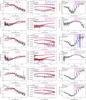 |
Fig. A.1 Flux (left panels), squared visibility amplitudes (middle panels), and closure phases (right panels) of R Cnc from data sets no. 1 to 6 (top to bottom) of Table 1 (black lines). Also shown are model predictions from the best-fit 1D CODEX (blue lines) and 3D CO5BOLD (red lines) models from Table 3. The squared visibility amplitudes include three lines that correspond to the three baselines of each AMBER dataset. Mean error bars are drawn in the center of each third of the total wavelength range. In particular, for the logarithmic scales, these are sometimes too small to be easily visible. They are typically 5–20% for the fluxes, 5–15% for the squared visibility amplitudes, and 5–15 deg for the closure phases. |
All Tables
All Figures
|
Fig. 1 Visual lightcurves of our sources as a function of Julian Date (top axis) and variability phase (bottom axis) around the dates of observation. The solid line denotes a sinusoidal fit to the data (crosses) obtained from the AAVSO and the AFOEV databases. The vertical dashed lines indicate the epochs of our observations. |
| In the text | |
|
Fig. 2 Direct comparison of (left) the visibility function and (right) the closure phases of data obtained of the same source at virtually the same baseline length and angle but at different epochs. From top to bottom: data sets 1&6 of R Cnc, 2&4 of R Cnc, 9&11 of X Hya, cf. Table 1. Errors of the squared visibility amplitudes are in the range of 5–15%; errors of the closure phases are in the range of 5–15 deg. |
| In the text | |
|
Fig. 3 Left panels: intensity profiles of (blue) the 1D CODEX model o54/286100 compared to (red) the azimuthally averages intensity profiles of snapshot 68 of the RHD simulation st28gm06n06 at bandpasses (from top to bottom) 2.00 μm–2.01 μm (water vapor), 2.25 μm–2.26 μm (continuum), 2.2934 μm–2.2936 μm (CO 2−1), and 2.47 μm–2.48 μm (CO). Both models provide a satisfactory fit to our visibility data of o Cet obtained in October 2012. The purple dashed line indicates a UD as reference. The intensities are normalized so that the integrated flux of each curve is unity. Right panels: images of the 3D intensity maps of snapshot 68 at the same bandpasses. A squareroot color scale is used to enhance the low intensities of the extended molecular atmosphere. |
| In the text | |
|
Fig. 4 Location of our sources in the HR diagram as listed in Table 7, together with those of the CODEX models and the 3D model st28gm06n06. Shown are the positions of individual CODEX models with different symbols for each of the four series, where the orange symbols represent the locations of the hypothetical non-pulsating parent star. The orange symbol and error bars of the 3D model denote the average and standard deviation of different snapshots of the 3D model. Individual snapshots of the 3D model are not shown. Also shown are stellar evolutionary tracks of the early AGB from Lagarde et al. (2012) for 1.0, 1.25, 1.5, and 2.0 solar masses and solar chemical composition. |
| In the text | |
|
Fig. A.1 Flux (left panels), squared visibility amplitudes (middle panels), and closure phases (right panels) of R Cnc from data sets no. 1 to 6 (top to bottom) of Table 1 (black lines). Also shown are model predictions from the best-fit 1D CODEX (blue lines) and 3D CO5BOLD (red lines) models from Table 3. The squared visibility amplitudes include three lines that correspond to the three baselines of each AMBER dataset. Mean error bars are drawn in the center of each third of the total wavelength range. In particular, for the logarithmic scales, these are sometimes too small to be easily visible. They are typically 5–20% for the fluxes, 5–15% for the squared visibility amplitudes, and 5–15 deg for the closure phases. |
| In the text | |
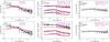 |
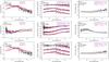
Fig. A.2 As Fig. A.1, but for W Vel, data sets No. 7 and 8 from Table 1. |
| In the text | |
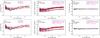 |
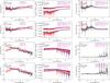
Fig. A.4 As Fig. A.1, but for R Aqr, data set No. 12 and 13 from Table 1. |
| In the text | |
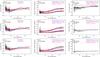 |
Fig. A.6 As Fig. A.1, but for R Leo, data sets No. 18–20 from Table 1. |
| In the text | |
Current usage metrics show cumulative count of Article Views (full-text article views including HTML views, PDF and ePub downloads, according to the available data) and Abstracts Views on Vision4Press platform.
Data correspond to usage on the plateform after 2015. The current usage metrics is available 48-96 hours after online publication and is updated daily on week days.
Initial download of the metrics may take a while.