| Issue |
A&A
Volume 587, March 2016
|
|
|---|---|---|
| Article Number | A97 | |
| Number of page(s) | 12 | |
| Section | Interstellar and circumstellar matter | |
| DOI | https://doi.org/10.1051/0004-6361/201526015 | |
| Published online | 24 February 2016 | |
The Musca cloud: A 6 pc-long velocity-coherent, sonic filament ⋆,⋆⋆
1 Department of Astrophysics, University of Vienna, Türkenschanzstrasse 17, 1180 Vienna, Austria
e-mail: alvaro.hacar@univie.ac.at
2 Max-Planck Institute für Astronomie, Königstuhl 17, 69117 Heidelberg, Germany
3 Observatorio Astronomico Nacional (OAN-IGN), Alfonso XII 3, 28014, Madrid, Spain
Received: 3 March 2015
Accepted: 19 November 2015
Filaments play a central role in the molecular clouds’ evolution, but their internal dynamical properties remain poorly characterized. To further explore the physical state of these structures, we have investigated the kinematic properties of the Musca cloud. We have sampled the main axis of this filamentary cloud in 13CO and C18O (2–1) lines using APEX observations. The different line profiles in Musca shows that this cloud presents a continuous and quiescent velocity field along its ~6.5 pc of length. With an internal gas kinematics dominated by thermal motions (i.e. σNT/cs ≲ 1) and large-scale velocity gradients, these results reveal Musca as the longest velocity-coherent, sonic-like object identified so far in the interstellar medium. The transonic properties of Musca present a clear departure from the predicted supersonic velocity dispersions expected in the Larson’s velocity dispersion-size relationship, and constitute the first observational evidence of a filament fully decoupled from the turbulent regime over multi-parsec scales.
Key words: radio lines: ISM / ISM: clouds / ISM: kinematics and dynamics / ISM: molecules / ISM: structure
This publication is based on data acquired with the Atacama Pathfinder Experiment (APEX). APEX is a collaboration between the Max-Planck-Institut fuer Radioastronomie, the European Southern Observatory, and the Onsala Space Observatory (ESO programme 087.C-0583).
The reduced datacubes as FITS files are only available at the CDS via anonymous ftp to cdsarc.u-strasbg.fr (130.79.128.5) or via http://cdsarc.u-strasbg.fr/viz-bin/qcat?J/A+A/587/A97
© ESO, 2016
1. Introduction
Since the earliest molecular line observations, it is well established that the internal gas kinematics of molecular clouds is dominated by supersonic motions (e.g., Zuckerman & Palmer 1974). These motions give rise to an empirical correlation between the velocity dispersion and the size-scale in molecular clouds, the so-called Larson’s relation (Larson 1981). In our prevalent paradigm of the turbulent interstellar medium (ISM; e.g., McKee & Ostriker 2007), this correlation arises from the power-law scaling of kinetic energy expected in a Kolmogorov-type cascade for a turbulence dominated fluid. As part of the turbulence decay, the density fluctuations created as a result of the supersonic gas collisions at distinct scales are responsible for the formation of the internal substructure of these objects (see Elmegreen & Scalo 2004, for a review).
Identifying the first (sub-)sonic structures formed inside molecular clouds is of fundamental importance to understanding their internal evolution. In the absence of supersonic compressible motions, the maximum extent of these sonic regions defines the end of the turbulent regime and the transitional scales at which turbulence ceases to dominate the structure of the cloud. From the analysis of the gas velocity dispersion in molecular line observations, Goodman et al. (1998) and Pineda et al. (2010) identified the dense cores as the first sonic structures decoupled from the turbulent flow, typically on scales of ~0.1 pc. More recently, Hacar & Tafalla (2011) have shown that these dense cores are embedded in distinct ~0.5 pc length, velocity-coherent filamentary structures, referred to as fibers, with identical sonic-like properties to those previously measured in cores. According to these latest results, the presence of this sonic regime precedes the formation of cores extending up to (at least) subparsec scales.
The interpretation of the supersonic motions reported in more massive filaments at larger scales is, however, matter of a vigorous debate. The ubiquitous presence of filaments in both star-forming and pristine molecular clouds revealed by the latest Herschel results indicates that their formation is particularly favored as part of the turbulent cascade (André et al. 2010, 2014). From the comparison of different clouds, Arzoumanian et al. (2013) has suggested that the internal velocity dispersion of those gravitationally bound filaments increases with their linear mass as a result of their gravitational collapse. On the other hand, Hacar et al. (2013) have demonstrated that supercritical filaments like the 10 pc long B213-L1495 region in Taurus are actually complex bundles of fibers. In these bundles, the apparent broad and supersonic linewidths are produced by the line-of-sight superposition of multiple and individual sonic-like structures at distinct velocities. New observations are needed to clarify this controversy.
In this paper we report the analysis of the internal gas kinematics of the Musca cloud (α, ) as a paradigmatic example of a pristine and isolated filament. With an estimated distance of ~150 pc derived from extinction measurements (Franco 1991), Musca is located at the northern end of the Musca-Chamaleonis molecular complex. As a characteristic feature, Musca exhibits an almost perfect rectilinear structure along its total length of more than 6 pc (see Fig. 1). Kainulainen et al. (2009) showed that the column density distribution of Musca has a shape more typical for star-forming than non-star-forming clouds. Yet, the cloud contains only a few solar masses at densities capable for star formation Kainulainen et al. (2014), suggesting that it may be in transition between quiescence and star formation (cf. Kainulainen et al. 2016). Indeed, early studies of this cloud have reported the presence of a single embedded object, IRAS12322-7023 (a TTauri candidate source), and a handful of dense but still prestellar, cores (Vilas-Boas et al. 1994; Juvela et al. 2012). Optical (Arnal et al. 1993; Pereyra & Magalhães 2004) and dust polarization (Planck Collaboration Int. XXXIII 2016) measurements have revealed the striking configuration of the magnetic field in this region which is perpendicularly oriented to the main axis of this filament. Large-scale extinction and submillimeter continuum maps indicate that its mass per unit length is similar to the value expected for a filament in hydrostatic equilibrium (Kainulainen et al. 2016). Additionally, millimeter line observations along this cloud have reported some of the narrowest lines detected in molecular clouds (Arnal et al. 1993; Vilas-Boas et al. 1994). These extraordinary physical properties make Musca an ideal candidate to explore the dynamical state of a filament in its early stages of evolution.
2. Molecular line observations
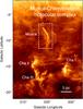 |
Fig. 1 Planck 857 GHz emission map, oriented in Galactic coordinates, of the northern part of the Musca-Chamaeleonis molecular complex. The different subregions are labeled in the plot. Note the favourable properties of the Musca filament, showing a quasi-rectilinear geometry along its ~6 pc of length, perfectly isolated from the rest of the complex. |
Between May and June 2011, we surveyed a total of 300 independent positions along the Musca cloud using the APEX12m telescope. As illustrated in Fig. 2 (left), the observed points correspond with a longitudinal cut along the main axis of the Musca filament. Designed to optimize the observing time on source, this axis follows the highest column density crest of this filament and the most prominent features identified in both extinction and continuum maps (Kainulainen et al. 2016). This axis was sampled every ~30 arcsec, corresponding to a typical separation of approximately one beam at the frequency of 219 GHz (Θmb = 28.5 arcsec).
In order to cover both transitions simultaneously, the APEX-SHeFI receiver was tuned to the intermediate frequency between the 13CO (J = 2−1) (ν = 220 398.684 MHz; Cazzoli et al. 2004) and C18O (J = 2−1) (ν = 219 560.358 MHz; Cazzoli et al. 2003) lines. All the observations were carried out in Position-Switching mode using a similar OFF position for all the spectra with coordinates (α, ), selected from the large-scale extinction maps of Kainulainen et al. (2009) as a position presenting extinctions values of AV< 0.5mag. To improve the observing efficiency, and in collaboration with the APEX team, a new observing technique was developed for this project where each group of 3 individual positions (not necessarily aligned) shared a single OFF integration, similar to the method using in raster maps. The typical integration time per point was set to 2 min on-source, while all the observations were carried out under standard weather conditions (PWV < 3 mm). Pointing and focus corrections and line calibrations were regularly checked every 1−1.5 h.
As results of an instrumental upgrade in June 2011, two distinct backends were used for this project. Approximately half of the positions were surveyed using the now decommissioned Fast Fourier Transform Spectrometer (FFTS) with an effective spectral resolution of 122 KHz or ~0.17 km s-1 at the central frequency of 220 GHz. The second half of these observations were carried out using the new facility RPG eXtended bandwidth Fast Fourier Transform Spectrometer (XFFTS) backend with an improved resolution of 76 kHz or ~0.10 km s-1 at the same frequencies. To check the consistency between the two datasets, eight of the most prominent positions along the filament were observed in both configurations. A systematic difference of 80 kHz (or ~0.10 km s-1) was found between the signal detected in both FFTS and XFFTS backends, which was attributed to hardware problems in the previous FFTS installation (C. DeBreuck, priv. comm.). This frequency correction was then applied to the final sample of FFTS data.
The final data reduction included a combination of the two datasets, where the XFFTS spectra were smoothed and resampled into the FFTS resolution in those positions were both observations were available, and a third-order polynomial baseline correction using the CLASS software1. To achieve this, each individual 13CO and C18O spectrum was reduced independently. According to the facility-provided antenna parameters included in the APEX website2, a final intensity calibration into main-beam temperatures was achieved by applying a beam efficiency correction of ηmb = 0.75. The resulting spectra present a typical rms value of 0.14 K.
3. Data analysis
3.1. Data overview
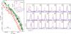 |
Fig. 2 Left: total column density map derived from NIR extinction measurements (Kainulainen et al. 2016). The contours are equally spaced every 2 mag in AV. The 300 positions surveyed by our APEX observations in both the 13CO and C18O (2–1) lines are marked in green following the main axis of this filament. The red star in the upper left corner denotes the position of the TTauri IRAS12322-7023 source. Right: 13CO (2−1) (red) and C18O (2−1) (blue; multiplied by 2) line profiles found in different representative positions along this cloud (spectra 1−18), all labeled on the map. The averaged spectra of all the data available inside this region are also shown in the upper right corner of the extinction map. |
Figure 2 (right) illustrates several representative 13CO and C18O (2−1) spectra found along Musca. As seen in the corresponding average spectra (upper right corner, in the left panel), the total emission of both lines appears at velocities between ~1.5 and 4.5 km s-1 with a smooth and continuous variation along the total ~6 pc of this filament (see spectra 1−18). Most of the observed positions present narrow lines with a prevalence of single-peaked spectra in both CO isotopologues. The observed velocity variations are consistently traced in both CO lines (see also Sect. 4.2). These kinematic properties reproduce the results obtained in the 13CO and C18O (1−0) observations carried out by Vilas-Boas et al. (1994) at different positions along Musca. Compared to the limited sample of 16 points studied by these authors, however, our survey of 300 observations allows us to investigate the dynamical state of this filament in detail.
A simple inspection of the individual line profiles found along the Musca filament reveals some of its particular kinematic features. Some C18O (2−1) spectra present total linewidths of less than two channels (e.g. spectra 12 and 15 in Fig. 2), being unresolved by our high spectral resolution observations. Additionally, most of these observed positions present a single component in velocity. Three well-defined regions contain most of the double-peaked spectra, typically detected in 13CO. The most prominent one is located at the northern end of Musca, coincident with the position of the IRAS12322-7023 source. The emission appears as a double-peaked line in 13CO and typically as a single line with a blue-shifted wing in C18O (see spectrum 18). Restricted to the vicinity of this IRAS source, this complex kinematics appears to be related to the interaction of this embedded object with its envelope.
Most of the double-peaked spectra detected in C18O are preferentially located at the southern end of Musca extending throughout a region of about 10 arcmin in length. In this case, two velocity components are detected in both 13CO and C18O isotopologues with roughly similar line ratios (see spectrum 1) suggesting a superposition of a secondary component along this region. A much clearer example of this behavior is found in the third of these regions, located at the intersection of what appears to be two independent branches identified in the central part of the Musca filament according to our extinction maps (Kainulainen et al. 2016,see also spectra 13 and 14).
This simple kinematic structure contrasts with the high level of complexity found in more massive bundle-like structures like B213-L1495 that ahve spectra characterized by high-multiplicity and high spatial variability (Hacar et al. 2013). Opposite to it, Musca resembles some of the quiescent properties of the single velocity-coherent fibers observed at scales of ~0.5 pc in regions like L1517 (Hacar & Tafalla 2011). Compared to these last objects, the quiescent nature of Musca seems to extend up to scales comparable to the total length of this cloud. In addition to its extraordinary rectilinear geometry, these observations suggest that Musca is the simplest molecular filament ever observed.
3.2. Gaussian decomposition
Following the analysis techniques used by Hacar & Tafalla (2011) and Hacar et al. (2013), we parametrized all the kinematic information present in our 13CO and C18O data by fitting Gaussians to all our spectra using standard CLASS routines. For that purpose, each individual spectrum was examined and fitted independently. In most cases, one single component was used at each individual position. A maximum of two independent components were fitted only if the spectrum presented a clear double-peaked profile whose two maxima were separated by at least three channels in velocity (e.g. spectrum 1 in Fig. 2). In case of doubt (i.e. top-flat or wing-like spectra; e.g. spectrum 5), one line component was fitted. This conservative approach was preferred to prevent the split of the line emission into artificially narrow subcomponents.
From the total of 300 spectra fitted for each line, ~80% of the 13CO and 95% of the C18O line profiles were identified and fitted as single-peak spectra with a signal-to-noise ratio S/N ≥ 3. The other 20% in the case of 13CO and 5% of the C18O spectra were fitted with two independent components. Most of the fitted profiles, either in single or multiple spectra, appear to be well reproduced by Gaussian components. With perhaps the exception of the wing-like emission around IRAS12322-7023 (i.e. spectrum 18), our Gaussian decomposition seems to capture the main kinematic properties of the gas traced by the two CO lines studied in this paper.
4. Results
4.1. Gas properties: temperature, column density, and molecular abundances
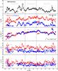 |
Fig. 3 Observational results combining both NIR extinction (black) and both 13CO (red triangles) plus C18O (blue squares) (2−1) line measurements along the main axis of Musca. From top to bottom: (1) extinction profile obtained by Kainulainen et al. (2016); (2) CO main-beam brightness temperatures (Tmb); (3) centroid velocity (Vlsr); (4) non-thermal velocity dispersion along the line of sight (σNT); and (5) opacity corrected non-thermal velocity dispersion along the line of sight (σNT,corr) including upper limits for the 13CO emission (red arrows; see text for discussion). The velocity dispersion measurements are expressed in units of the sound speed cs = 0.19 km s-1 at 10 K. In these last plots the horizontal lines delimitate to the sonic (σNT/cs ≤ 1; thick dashed line) and transonic (σNT/cs ≤ 2; thin dotted line) regimes, respectively. Only those components with a S/N ≥ 3 are displayed in the plot. The position of the IRAS 12322-7023 source as well as a typical 3 km s-1 pc-1 velocity gradient are indicated in their corresponding panels. We note the presence of the double-peaked spectra at the positions Lfil ~ 0.4,4.2, and 5.8 pc in the middle panel. The two vertical lines delimitate the south, central, and north subregions identified by Kainulainen et al. (2016). |
Owing to the observed differences in their integrated intensity maps, the most abundant CO isotopologues are commonly interpreted as density selective tracers: 12CO and 13CO seem to trace the most diffuse gas in clouds while only C18O is detected in regions with highest column- and volume densities. This interpretation relies on the oversimplified assumption that the expected fractional abundances of these molecular tracers (e.g. X(C18O):X(13CO):X(12CO) = 1:7.3:560; Wilson & Rood 1994) are translated into differential sensitivity thresholds for the distinct density regimes in clouds. Physically speaking, however, all the CO isotopologues share quasidentical properties in terms of their excitation conditions and chemistry. If secondary effects like radiative trapping (Evans 1999) and photodissociation within self-shielded regions (AV> 2−3; van Dishoeck & Black 1988) are neglected, these molecular tracers should be sensitive to roughly the same gas at all densities and along the same line of sight. Observationally, this picture is complicated by the different emissivities and optical depths of their lower-J rotational transitions. Thanks to their large relative abundances, the detection of the most abundant isotopologues (i.e., 12CO and 13CO) is favored over their rarest counterparts (e.g., C18O or C17O) particularly in the diffuse outskirts of the clouds. In addition, these large relative abundances also produce strong variations in their line opacities (i.e., τ(A) ~ X(A/B)·τ(B) for the same J-transition; Myers et al. 1983a). As a result, tracers like 12CO or, to lesser extent, 13CO become heavily saturated in regions with high column densities.
The combination of multiple CO lines can be used to derive different physical properties of the molecular gas inside clouds (e.g., Myers et al. 1983a; Vilas-Boas et al. 1994). The three main parameters derived from our Gaussian fits with S/N ≥ 3 (i.e., peak line temperature, velocity centroids, and velocity dispersion) are presented in Fig. 3 as a function of the position along the main axis of the Musca filament (Lfil) measured from the southern end of this cloud. For comparison, this figure (first panel) includes the near-IR (NIR) extinction values derived along the same axis (Kainulainen et al. 2016). The first of the parameters studied there corresponds with the observed line intensity or brightness temperature Tmb (second panel). Values for Tmb of 5−7 K and 1−3 K are found for the 13CO and C18O (2−1) components, respectively. Compared to the canonical line ratio of 7.3 expected in the optically thin case, a point-to-point comparison shows characteristic values of Tmb(13CO)/Tmb(C18O)~ 5, indicative of moderate opacities for the 13CO (2−1) lines (see below). In the optically thick approximation, the observed line intensities lead to excitation temperatures of Tex(13CO) = 9−11 K. These results are in close agreement with the average gas kinetic temperatures found in starless cores (TK ~10 K; Benson & Myers 1989) and the dust effective temperatures reported for the two most prominent starless cores observed in Musca (Tdust = 11.3 K; Juvela et al. 2010) (cores 4 and 5 according to Kainulainen et al. 2016 notation). For practical purposes, in this paper we have assumed LTE excitation conditions with a uniform gas kinetic temperature of TK = 10 K for all the gas traced by our CO observations (i.e. Tex(13CO) = Tex(C18O) = 10 K).
At each position observed along the Musca cloud, we have estimated the central optical depth τ0 of the C18O (2−1) emission from the peak temperatures measured in our spectra as: 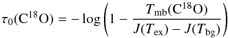 (1)obtained solving the radiative transfer equation where
  (e.g., Rohlfs & Wilson 2004). Figure 4 presents the linear increase of the resulting C18O (2−1) line opacity as a function of the extinction values reported by Kainulainen et al. (2016) at the same positions. At those column densities where this molecule is detected, we obtain opacity values of τ(C18O(2−1)) = 0.08−1.3. Assuming standard CO fractionation, this optically thin C18O emission yields optically thick estimates of τ(13CO(2−1)) = 0.5−9.5 and, although not observed here, τ(12CO(2−1)) ~ 30−400.
The different line opacities of the 13CO and C18O lines are recognized in several of the parameters derived in our fits. Figure 4 (Mid panel) presents the evolution of the C18O column densities, estimated in LTE conditions from the integrated intensity of these lines as a function of AV. As expected for an optically thin tracer with constant abundance, a linear correlation is recovered between these two observables. In absolute terms, the CO abundances derived from the C18O column densities obtained in Musca are consistent, within a factor of 2, with the values found in clouds like Taurus and Ophiuchus (i.e., X(C18O/H2) ~ 1.7 × 10⁻⁷; see Fig. 4; Frerking et al. 1982). Instead, the increasing line opacity of the 13CO lines is reflected in the monotonic decrease of the Tmb(13CO)/Tmb(C18O) line ratio found at AV ≳ 4 in Fig. 4 (lower panel). Their canonical abundance ratio is recovered when each of these lines (in particular the optically thick 13CO) are corrected by their corresponding opacity (i.e.  ; Goldsmith & Langer 1999). At the opposite end, the selective photodissotiation of the less abundant C18O molecules is most likely responsible for the observed increase on the Tmb(13CO)/Tmb(C18O) line ratio below AV< 3 mag (see van Dishoeck & Black 1988, for a discussion). As detailed in Sect. 4.3, these saturation effects also produce a non-negligible contribution to the observed linewidths of optically thick tracers like 13CO.
Although sporadically found at lower extinctions, the C18O emission is primarily detected at AV ≳ 3−4 mag. Supplemented by our 13CO spectra down to AV ≳ 2 mag (see Fig. 3, top panel), the current sensitivity of our APEX observations limits our observation to equivalent total gas column densities of N(H) ≳ 3.8 × 1021 cm-2 (assuming a standard conversion factor of N(H)(cm-2) = 1.9 × 10²¹AV (mag); Savage et al. 1977). This detection threshold corresponds to the areas within the first contour of the extinction map presented in Fig. 2 (left). According to Kainulainen et al. (2016), ~50% of the total mass of the cloud (defined within a total extinction contour of AV ~ 1.5 or N(H) = 2.9 × 1021 cm-2) is contained at these column densities. Due to the limited coverage of our survey, the above value is assumed as an upper limit of the cloud mass fraction traced by our CO observations.
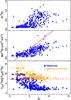 |
Fig. 4 Observational properties of the observed C18O and 13CO (2−1) lines as a function of the total column density observed along the Musca filament: (upper panel) optical depth of the C18O (2−1) lines; (mid panel) C18O total column density; (lower panel) observed (blue solid squares) and opacity corrected (orange diamonds) Tmb(13CO)/Tmb(C18O) line ratio. The gray dashed line in the upper panel corresponds to the characteristic detection S/N = 3 line detection threshold for a spectrum with an rms value of 0.14 K, in Tmb units. The derived C18O column densities are consistent (within a factor of two) with the typical abundances obtained in clouds like Taurus and Ophiuchus (solid red line in the mid panel; Frerking et al. 1982). The red horizontal line in the lower panel indicates the canonical Tmb(13CO)/Tmb(C18O) = 7.3 line ratio expected in an optically thin regime. |
4.2. A 6-pc-long, sonic filament
Figure 3 (third panel) presents the velocity variations along the main axis of Musca determined from the velocity centroid (Vlsr) of the 13CO and the C18O (2−1) lines. Statistical values of ⟨ | Vlsr(C18O)−Vlsr(13CO) | ⟩ = 0.08 ± 0.07 km s-1, where 68% of these points with absolute differences within the velocity resolution of our spectra (i.e. | Vlsr(C18O)−Vlsr(13CO) | ≤ 0.1 km s-1), denote the close correlation that exist between the velocity fields traced by our CO data in those positions where the emission of both isotopologues are detected. Despite some exceptional regions identified in the double-peaked spectra described before, the velocity structure of Musca is characterized by a continuous and unique velocity component. At large scales, Musca presents a longitudinal and smooth south-north velocity gradient corresponding to ∇Vlsr | global ~ 0.3 km s-1 pc-1. With similar values to those previously reported from the study of the 12CO (1–0) emission at large scales by Mizuno et al. (2001) (∇Vlsr | global(12CO) ~ 0.2 km s-1 pc-1), these global velocity gradient seems to originate in the diffuse gas, being inherited by this filament during its formation. Locally, and at subparsec scales, the velocity field of Musca is dominated by higher magnitude velocity gradients with values of ∇Vlsr | local ≲ 3 km s-1 pc-1. Some of these local gradients appear as oscillatory motions associated with the positions of the most prominent cores in Musca (e.g.; Cores 4 & 5 in Kainulainen et al. 2016) (see also Sect. 4.5). With characteristic amplitudes of ~0.25 km s-1, these wavy velocity excursions resemble the streaming motions associated with the formation of cores within the L1517 filaments (Hacar & Tafalla 2011).
The third quantity determined in our Gaussian fits is the full width half maximum of the line (ΔV). For each molecular species i (either 13CO or C18O), the non-thermal velocity dispersion along the line of sight (σNT) can be directly obtained from this observable after subtracting in quadrature the thermal contribution to the line broadening as:  (2)where
  defines the thermal velocity dispersion of each of these tracers with a molecular weight m, determined by the gas kinetic temperature TK. Measurements of σNT are commonly expressed in units of the H2 sound speed (i.e., σth(H2,10 K) = cs = 0.19 km s-1, for μ = m(H2) = 2.33). This ℳ = σNT/cs ratio defines the observed Mach number ℳ classically used to distinguished between the sonic (ℳ ≤ 1), tran-sonic (1 < ℳ ≤ 2), and supersonic (ℳ > 2) hydrodynamical regimes in isothermal, non-magnetic fluids.
The different values of the non-thermal velocity dispersion measured along the Musca cloud in both 13CO and C18O lines are presented in Fig. 3 (fourth panel) in units of the sound speed cs at TK = 10 K. As seen there, each of the CO isotopologues exhibits a roughly constant σNT along the whole region sampled in our survey. A mean tran-sonic value of ⟨σNT/cs⟩ = 1.45 is obtained from the direct measurements of the 13CO linewidths (see also Sect. 4.3). More extreme is the case of the C18O (2−1) lines. With ⟨σNT/cs⟩ = 0.73, the emission detected in this last isotopologue presents an overwhelming fraction of ~85% of subsonic points and a maximum transonic velocity dispersion of σNT/cs = 1.7.
The quiescent properties of the gas velocity field of Musca (i.e. continuity, internal gradients, oscillatory motions, and velocity dispersions) mimic the kinematic properties found in the so-called velocity-coherent fibers, previously identified in Taurus (Hacar & Tafalla 2011; Hacar et al. 2013). Nevertheless, and in comparison to the 0.5 pc long fibers, the velocity-coherence of Musca extents up to scales comparable to the total size of the cloud. With a total length of 6.5 pc, Musca is, therefore, the largest sonic-like, velocity-coherent structure identified in the ISM so far.
4.3. Opacity broadening: observed linewidths and true velocity dispersions
The so-called curve of growth of a molecular line describes the relationship between the intrinsic (ΔVint) and the observed (ΔV) linewidths as a function of its central optical depth τ0 (e.g., Phillips et al. 1979): ![\begin{equation} \label{eq:broad} \beta_\tau=\frac{\Delta V}{\Delta V_{\rm int}} =\frac{1}{\sqrt{\ln 2}}\left[\ln \left( \frac{\tau_0}{\ln\left(\frac{2}{\exp(-\tau_0)+1} \right) } \right) \right]^{1/2}\cdot \end{equation}](/articles/aa/full_html/2016/03/aa26015-15/aa26015-15-eq89.png) (3)This equation asymptotically converges to
(3)This equation asymptotically converges to  for τ0 ≫ 1. Using Eq. (3) it is easy to prove how this opacity broadening dominates the observed linewidths for τ0> 10 (≥50%). While its effects can be neglected in the case of optically thin lines like C18O (τ0< 1Vilas-Boas et al. 1994), this opacity broadening significantly contributes to the observed linewidths of the low-J13CO (1 ≲ τ0< 10) and, in particular, 12CO transitions (τ0 ≳ 100). Thus, these opacity effects must be properly subtracted in order to compare the gas kinematics traced by the different CO isotopologues (see a detailed discussion in Hacar et al. 2015).
Figure 3 displays the non-thermal velocity dispersions σNT and σNT,corr obtained from both observed ΔV (fourth panel) and intrinsic ΔVint linewidths (i.e. according to Eqs. (2) and (3); fifth panel), respectively. We carried out this comparison where the line opacities of the C18O data were available. Otherwise, the observed σNT for 13CO were assumed as an upper limit of the true velocity dispersion of the gas. Statistically speaking, the mean contribution of the opacity broadening is estimated to be less than 5% in the case of the optically thin C18O linewidths and in ~25% for the moderately opaque 13CO lines. Remarkably, and after these opacity corrections, the gas traced in 13CO in different subregions within the Musca filament (e.g., 1.5 ≤ Lfil(pc) ≤ 4.8) present sonic-like velocity dispersions with ⟨ σNT,corr(13CO)/cs ⟩ = 1.0. Overall, the opacity corrected 13CO lines still present a larger non-thermal velocity dispersion than their corresponding C18O counterparts, indicative of an increase of the turbulent motions towards the cloud edges at AV< 3−4 mag. However, and while measurable differences are still present in the gas kinematic traced by each of these CO lines, their discrepancies are restricted to changes of less than a factor of two in absolute terms and within the (tran-)sonic regime.
According to Eq. (3), these opacity broadening effects account for ≳60% of the observed linewidths in the case of highly opaque lines like the low-J12CO transitions (τ0 ≳ 100). Values in the range of ΔV(12CO(2−1)) ~ 0.9−1.3 km s-1 are then estimated for the expected 12CO lines in Musca with intrinsic non-thermal velocity dispersions of ⟨ σNT,corr/cs ⟩ = 0.5−1.0, similar to the values deduced from our C18O and 13CO spectra. Thus, the opacity line broadening might be also responsible for part of the observed 12CO(1−0) linewidths reported in previous molecular studies along the main axis of this cloud with ΔV(12CO(1−0)) = 1.0−1.5 km s-1 (Arnal et al. 1993; Mizuno et al. 2001, H. Yamamoto, priv. comm.).
4.4. Microscopic vs. macroscopic motions
As discussed by Larson (1981), the total internal velocity dispersion of a cloud is determined by the combined contribution of the large-scale velocity variations and both the small-scale non-thermal and the thermal motions. The simple kinematic and geometrical properties of Musca allow us to isolate and study each of these components individually. The first two can be directly parametrized from the values measured in both the dispersion of the line velocity centroids σ(Vlsr) and the non-thermal velocity dispersions σNT. With a roughly constant temperature distribution according to Sect. 4.2, we then obtain values of { σ(Vlsr),σNT,σth(H2) } = { 1.9,0.7,1.0 } × cs from the C18O (2−1) and { 2.2,1.5,1.0 } × cs from the 13CO (2−1) lines (without opacity corrections). While in all the cases the observed dispersions are typically (tran-)sonic (i.e. ≲ 2cs), the comparison of these individual components indicates that the global dispersion inside Musca cloud is dominated by the contribution of the macroscopic velocity variations along this cloud.
The nature of these macroscopic motions is also revealed by the continuity of the velocity field observed in Musca. As seen in Fig. 3 (third panel), the total velocity dispersion σ(Vlsr) results from the combination of both local velocity excursions plus large-scale and global motions along the main axis of this filament (see also Sect. 4.5). Compared to the random microscopic velocity variations (e.g. thermal velocity dispersion), our observations demonstrate that the largest velocity differences observed in Musca should be attributed to the presence of systematic and ordered (i.e. highly anisotropic) motions inside this cloud.
4.5. Structure function in velocity: local oscillations vs. large-scale gradients
Model description and parameters.
The macroscopic motions inside clouds are primarily determined by the combination of velocity oscillations and large-scale velocity gradients. In this section we aim to quantify their relative contribution to the total velocity field in Musca from the analysis of the variations of the line-centroids using the velocity structure function: Sp(L) = ⟨ | v(r)−v(r + L) | p⟩. Among other correlation techniques (see Ossenkopf & Mac Low 2002,for a review), the structure function is used in molecular lines studies as a diagnostic of the velocity coherence at a given scale L (e.g., Miesch & Bally 1994). In practice, the structure function is commonly reframed as its pth root (i.e. Sp(L)1 /p) and described by its power-law dependency ∝ Lγ (see Heyer & Brunt 2004). The square root of the second-order structure function (i.e. S2(L)1 / 2) then yields  (4)where v0 and γ are the scaling coefficient and the power-law index, respectively. Tafalla & Hacar (2015) used measurements of δV to evaluate the velocity structure along different star-forming fibers in the B213-L1495 region. These authors demonstrated that the individual velocity-coherent fibers present flat and sonic-like structure functions (i.e. γ ~ 0 and v0 ~ cs) at scales of ≤0.5 pc. Intuitively, this behavior is expected as the result of the small velocity variations observed inside these fibers (i.e. Vlsr(r) ~ Vlsr(r + L)).
Compared to the short lags L sampled in the Taurus fibers, the study of δV in Musca can be extended up to multiparsec scales. Using Eq. (4), Fig. 5 displays the results for δV along the main axis the Musca cloud in bins of 0.15 pc. The values presented there are calculated for all the positions detected in 13CO belonging to the main gas velocity component of this cloud and not affected by the IRAS 12322 source (see Sect.3). Tracing the same kinematics, the use of 13CO is justified by the larger coverage and sensitivity of the emission of this tracer compared to C18O. Oscillations and gradients with similar magnitudes are characteristic of the gas velocity field both parallel and perpendicular to the main axis of filaments mapped using fully sampled 2D observations (Hacar & Tafalla 2011). A preliminary analysis of several cuts perpendicular to the axis of Musca observed in C18O are consistent with these results (Hacar et al., in prep.). Despite their limited coverage following the main axis of this cloud, our observations are considered a good descriptor of the gas velocity field within the gas column densities traced by our APEX observations.
A broken power-law behavior is observed in the structure function of Musca. Sharing again some of the properties of the fibers, an automatic linear fit at correlation lags L ≤ 1 pc within Musca produces a (tran-)sonic-like structure function (δV ~ 1−2cs; v0 = 0.32 km s-1) with a shallow power-law dependency γ = 0.25. Conversely, between L> 1 pc and the completeness limit of our study at ~3 pc (or Lfil/ 2), the structure function becomes supersonic (δV> 2cs) showing a steeper power-law index γ = 0.58 (with v0 = 0.38 km s-1). This rapid increase of the slope of the δV between these two well-defined regimes suggests a change in the internal velocity field of the Musca cloud at characteristic scales of ~1 pc.
Beyond their statistical description, the direct interpretation of spatial correlation techniques like δV is usually hampered by the morphological complexity of the clouds and the intrinsic limitations imposed by the use of projected measurements along the line of sight (Scalo 1984). The geometric simplicity of Musca offers a unique opportunity to explore the origin of the power-law dependency of the structure function at different scales for the case of 1D filamentary structures. For that purpose, we created a set of four numerical tests to reproduce the observed δV in filaments with different characteristic internal velocity fields (see Models 1−4 in Table 1). In all cases, we assumed these filaments as 6 pc long, 1D structures sampled every 0.022 pc, that is, similar to our APEX observations in Musca, showing a unique and continuos velocity component. The resulting position-velocity diagram of each of these models are displayed in Fig. 6 (left). First, Models 1 and 2 describe two idealized filaments presenting a pure sinusoidal velocity field and a global velocity gradient along their main axis, respectively. These two cases describe the most fundamental velocity modes reported in the study of the internal gas kinematics inside filaments (Hacar & Tafalla 2011). In addition, Model 3 is created by the linear combination of Models 1 and 2, defining a filament whose velocity field consists of a large-scale gradient superposed onto a small-scale oscillatory profile. Finally, Model 4 represents a generalized version of the previous three models where the internal kinematics of this filament is described by a linear gradient and a series of complex velocity excursions varying in period along its axis.
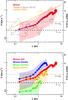 |
Fig. 5 Second-order structure function in velocity S2(L)1 / 2 = δV as a function of length L (i.e. lag) derived from our 13CO observations along the main axis of Musca (red points). Upper panel: analysis of the global velocity field within the Musca filament. For comparison, the results obtained by Tafalla & Hacar (2015) in four distinct velocity-coherent fibers in the B213-L1495 cloud are displayed in gray. The orange line denotes the Larson’s velocity dispersion-size relationship with δV = σ = 0.63 L0.38. Lower panel: structure function of the individual south (blue), center (green), and north (orange) subregions within Musca (see text) in comparison with the total cloud (red; similar to upper panel). The errors on the δV measurements are smaller than the point size. Instead, the shaded areas refer to the intrinsic dispersion of these measurements created by the combined contribution of the velocity excursions with different periods and the variations of the large-scale velocity gradients within this filament (see text). |
The resulting second-order structure function δV derived from Eq. (4) for the four model filaments are shown in Fig. 6 (right). These figures reveals that each individual component of the velocity field has a particular signature in shaping their corresponding structure function. Despite their apparent complexity, in most of the cases the individual δV can be reasonably fitted, in a first-order approximation, by simple analytic functions (see Table 2). The sinusoidal velocity excursions in Model 1 are translated into a roughly constant structure function. Different numerical tests show that the mean value of this structure function can be approximated to the amplitude of the oscillation A, that is, δV1(L) ~ A. In the case of Model 2, its analytic solution can be easily derived from Eq. (4), showing the linear dependency of δV(L)2 with the global gradient δV(L)2 = ∇Vlsr·L. On the other hand, the relative complexity in Model 3 can be described by the addition in quadrature of the contributions of both oscillatory and linear modes as ![\hbox{$\delta V(L)_3\sim [A^2+\nabla V_{\rm lsr}^2 \cdot L^2]^{1/2}$}](/articles/aa/full_html/2016/03/aa26015-15/aa26015-15-eq145.png) . In these simplified simulations, the inclusion of the more complex oscillations (i.e., with different periods) in Model 4 smooth out the shape of δV(L)4, although its average properties remain unaltered for reasonable input parameters in comparison with δV(L)3. Variations on the periodicity of the oscillations and, in a more general description, changes on the velocity gradients along the main axis of these filaments introduce an intrinsic dispersion in the structure function measurements in Model 4 (shaded areas in Fig. 6, lower-right panel). This intrinsic dispersion is correlated to the amplitude of the oscillations providing additional information to the velocity structure deduced from the mean values in these toy models. Due to the high accuracy of the line centroids obtained from our Gaussian fits (<0.01 km s-1) and the large number of pairs considered per bin (>500), the intrinsic (but still meaningful) spread of the structure function is at least an order of magnitude larger than the small nominal errors of these measurements.
. In these simplified simulations, the inclusion of the more complex oscillations (i.e., with different periods) in Model 4 smooth out the shape of δV(L)4, although its average properties remain unaltered for reasonable input parameters in comparison with δV(L)3. Variations on the periodicity of the oscillations and, in a more general description, changes on the velocity gradients along the main axis of these filaments introduce an intrinsic dispersion in the structure function measurements in Model 4 (shaded areas in Fig. 6, lower-right panel). This intrinsic dispersion is correlated to the amplitude of the oscillations providing additional information to the velocity structure deduced from the mean values in these toy models. Due to the high accuracy of the line centroids obtained from our Gaussian fits (<0.01 km s-1) and the large number of pairs considered per bin (>500), the intrinsic (but still meaningful) spread of the structure function is at least an order of magnitude larger than the small nominal errors of these measurements.
The results obtained from the models presented in Fig. 6 (right) illustrate their potential use in the study of the gas dynamics inside filaments. In particular, the behavior of δV(L)3 reveals the influence of the two fundamental velocity modes in the total velocity structure of these objects: while local velocity variations dominate the shape of δV at short correlation lags exhibiting a flat scale dependence (γ ~ 0), the presence of global velocity gradients produces a rapid increase of its slope at larger L values (γ → 1). Interestingly, the transition between these two regimes can be directly obtained from the parameters describing δV(L)3, estimated at scales of Λ = A/ ∇Vlsr (see also Fig. 6, Model 3).
Despite the obvious limitations of these toy models, their results closely reproduce the observed properties describing the gas velocity field within the B213-L1495 region. The internal velocity field of the fibers detected in this cloud is characterized by presenting typical velocity gradients of ∇Vlsr = 0.5 km s-1 pc-1 and velocity excursions with amplitudes of A ~ 0.2 km s-1 (Hacar et al. 2013). Only at scales of Λ ~ A/ ∇Vlsr = 0.2 / 0.5 > 0.4 pc is the velocity field of these B213-L1495 fibers then expected to be dominated by the contribution of their global velocity gradients. These results naturally explain the roughly flat structure functions obtained for these objects up to scales of ~ 0.5 pc (Tafalla & Hacar 2015; see also Fig. 5). In addition, our models also predict the broken power-law behavior observed in the structure function of Musca. As seen in Fig. 6, a similar dependence is reproduced in Models 3 and 4 assuming characteristic values of ∇Vlsr = 0.25 km s-1 pc-1, A = 0.25 km s-1, and T = 0.5 pc (see Table 1). In this last case, the change in the slope of δV(L) at Λ = 1 pc reveals the increasing influence of the global velocity gradient in the velocity differences observed inside this object at parsec scales. Based on these results, we then conclude that the supersonic velocity differences (or velocity dispersions) reported in the structure function of Musca are mostly created by the projection of these global motions along the main axis of this cloud.
From the analysis of its mass distribution based in extinction and continuum maps in this filament, Kainulainen et al. (2016) have suggested that Musca could be in the middle of its gravitational collapse. According to their internal substructure and number of embedded cores, these authors distinguished three subregions within this cloud: the almost unperturbed and pristine central part of Musca plus the highly fragmented north and south subregions (Fig. 3, first panel). The level of fragmentation (i.e., the magnitude of the dispersion measured in the column density maps) within each of these three subregions appears to be correlated with their internal velocity dispersion and local gradients. Kainulainen et al. interpreted these properties as the development of the gravitational fragmentation progressing from the cloud edges towards the center of this filament.
The set of parameters obtained above (A, ∇Vlsr, and Λ) describe the average properties of the gas velocity field within the Musca filament. Already in our data, significant differences are also observed within the three subregions identified by Kainulainen et al. (2016) within this cloud. In Fig. 5 (lower panel), we have obtained the structure function for each of these individual subregions. As for the whole cloud, we have described each of these new distributions using a broken power-law with two different slopes fitted by eye within their corresponding completeness limit. In close agreement with the values manually derived in the position-velocity diagrams of Fig. 3, this simple modeling captures most of the differences observed between the quiescent gas velocity field of the central region (A = 0.08 km s-1, ∇Vlsr = 0.15 km s-1 pc-1, Λ = 0.5 pc), and the combination of oscillations and gradients of different magnitudes present in the adjacent south (A = 0.25 km s-1, ∇Vlsr = 0.50 km s-1 pc-1, Λ = 0.5 pc) and north regions (A = 0.22 km s-1, ∇Vlsr = 0.20 km s-1 pc-1, Λ = 1.1 pc). The high sensitivity of our models to these local variations denote their potential as diagnostic tools of the gas velocity structure in 1D filamentary structures.
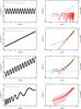 |
Fig. 6 Position velocity diagram (left; black dots) and its corresponding δV( = S2(L)1 / 2) structure function (right; red dots) for the four 1D filamentary clouds modeled in this work (see also Table 1). From top to bottom: (Model 1) Filament presenting a sinusoidal (i.e. oscillatory) velocity profile with amplitude A = 0.25 km s-1 and period T = 0.5 pc; (Model 2) filament presenting a longitudinal large-scale velocity gradient with ∇Vlsr = 0.25 km s-1 pc-1; (Model 3) filament presenting both a global velocity gradient and an oscillation with similar parameters to Models 1 and 2, respectively; (Model 4) filament presenting a global velocity gradient and a complex oscillatory profile with variable period. The green lines represent the analytical fit of their corresponding structure functions (see Table 2). In the case of Model 3, the vertical dashed line denotes the transitional scale where the global velocity gradient dominates over the local motions, estimated as Λ ~ A/ ∇Vlsr. For all plots, the blue dashed lines indicate the broken power-law dependency observed in Musca (see Fig. 5). Similar to our observations, we note that the completeness limit of δV is restricted to scales ≤3 pc (=Lfil/2) owing to the finite size of our models. The shaded area in the last panel indicates the intrinsic dispersion per bin introduced by the presence of multiple oscillations with different periodicity in Model 4. |
5. Discussion
5.1. Departure from Larson’s velocity dispersion-size relationship
The so-called Larson’s velocity dispersion-size relationship (often referred to as linewidth-size relationship) defines the observational correlation found between the velocity dispersion (σ) of the gas as a function of cloud size (L). Collecting data from the literature for different nearby clouds, Larson (1981) first pointed out that this relationship can be described by a power-law dependence σ(km s-1) ≃ CL(pc)Γ, with coefficients C = 0.63 and Γ = 0.38, respectively3. In later studies, roughly similar power-law behaviors were consistently reported for the velocity structure in both galactic (C = 1.0 and Γ = 0.5; Solomon et al. 1987) and extragalactic clouds (C = 0.44 and Γ = 0.6; Bolatto et al. 2008) along more than three orders of magnitudes in scale between ~0.1−100 pc . The small variations found in both C and γ parameters describing the Larson’s velocity dispersion-size relationship inside molecular clouds are interpreted as an observational signature of the universality of the ISM turbulence (Heyer & Brunt 2004).
As demonstrated by Heyer & Brunt (2004), the universal behavior of the velocity dispersion-size relationship based on cloud-to-cloud comparisons can only be explained if each of these individual objects presents a quasi-identical and Larson-like internal structure function (i.e., δV(L)i ~ σ(L) ∝ Lγ). Contrary to their conclusions, and as illustrated in Fig. 5 (upper panel) (see also Sect. 4.5), the observed power-law dependency of the δV(L) function in Musca systematically deviates from the Larson’s velocity dispersion-size predictions in both its slope and its absolute scaling coefficient, even when its intrinsic dispersion is considered. The two functions seem to converge only at large spatial correlation lags L> 3 pc. In Musca, however, these large velocity differences are produced by the presence of large-scale and ordered velocity gradients instead of by turbulent random motions (Sect. 4.5).
The flat structure function reported for the internal gas kinematics inside fibers at scales of ~0.5 pc was used by Tafalla & Hacar (2015) to prove the particular nature of these objects fully decoupled from the turbulent cascade. A similar conclusion can be drawn from the analysis of the δV(L) dependence observed in Musca at scales comparable with its total ~6.5 pc length. Large-scale departures from Larson’s predictions were previously suggested for individual filamentary objects like the Ophiuchus Streamers (Loren 1989). The detection of quiescent clouds like Musca indicate that some of these filaments could present an internal velocity dispersion deviating from Larson’s velocity dispersion-size relationship at parsec-scales. Without necessarily contradicting the global gas properties described by this last empirical relationship, our observations show that the local kinematics of some individual subregions within molecular clouds might not necessarily follow Larson’s predictions.
5.2. Origin of the Musca cloud
The results presented in this paper extend the size of the sonic regime of the gas inside filaments by about an order of magnitude compared to previous studies. Low-amplitude continuous longitudinal gradients seemed to be characteristic of fibers. However, the presence of similar velocity-coherent, sonic-like structures was thought to be restricted to subparsec scales (Hacar & Tafalla 2011; Hacar et al. 2013). The low velocity dispersion (Sect. 4.2), as well as the shallow dependency of its structure function (Sect. 4.5) indicate that no significant internal supersonic, turbulent motions are present in Musca at multiparsec scales.
The dynamical properties of Musca make its origin puzzling. Pure hydrodynamical simulations typically produce dense filamentary structures with low velocity dispersions in the post-shock regions after the collision of supersonic flows (e.g., Padoan et al. 2001). The almost ideal conditions required to produce an isolated, unperturbed parsec-scale filamentary structure like Musca in this shock-dominated scenario could explain the uniqueness of this object. Its elongated nature could also be favored by the presence of the highly ordered magnetic field structure reported in previous studies (Pereyra & Magalhães 2004). The orthogonal orientation of the magnetic field lines with respect to the main axis of Musca could promote the gravitational condensation of material towards its axis. According to magnetohydrodynamic simulations (e.g., Nakamura & Li 2008), this configuration would also inhibit the gas motions across the magnetic field lines, preventing or delaying the internal fragmentation along this cloud and leading to a slow and inefficient star formation inside Musca, in agreement with our observational results. These different formation scenarios will be explored with the analysis of the gas velocity field perpendicular to this filament in a future paper (Hacar et al., in prep.).
Our findings in Musca could potentially open a new window in the study of the evolution of filaments in molecular clouds. The intricate nature of more massive star-forming filaments, like B213-L1495 (Schmalzl et al. 2010; Hacar et al. 2013), complicates the detailed analysis of these objects and, in particular, their comparison to simulations. Far from this complexity, Musca could be used as benchmark of more simplified physical models (e.g., see Sect. 4.5). Thanks to its favorable structure, geometry, and kinematic properties, direct predictions for distinct key processes like the fragmentation and stability mechanisms in filaments could easily be tested in this cloud (e.g., Kainulainen et al. 2016). All these extraordinary properties make Musca an ideal laboratory for studying the nature and evolution of filamentary clouds.
6. Conclusions
We investigated the dynamical state of the Musca cloud using APEX submillimeter observations. We sampled 300 positions along the main axis of this filament in both 13CO and C18O (2−1) lines. We characterized the internal kinematic structure of Musca from the analysis of the different line profiles. The main conclusions of this work are as follows:
-
1.
The velocity structure of the Musca cloud is characterized by a continuous and quiescent velocity field along its total length of 6 pc. Its internal gas kinematics traced by the C18O (2−1) emission is mainly described by a single velocity component presenting (tran-)sonic non-thermal velocity dispersions (i.e., ⟨σNT/cs⟩ ≲ 1) and smooth and oscillatory-like velocity profile with internal velocity gradients of ∇Vlsr ≲ 3 km s-1 pc-1). Consistent results are obtained from the analysis of the 13CO (2−1) lines.
-
2.
The properties of the gas velocity field in Musca present similar characteristics to those reported in previous studies for the so-called velocity-coherent fibers at scales of ~0.5 pc. About an order of magnitude larger in extension, Musca is therefore the largest sonic-like structure identified so far in nearby clouds.
-
3.
The analysis of local and global motions indicates that the largest velocity variations inside Musca arise from the parsec-scale projection of a global velocity gradient along its main axis. Hence, the velocity field in this cloud is dominated by macroscopic, ordered, and systematic motions.
-
4.
We have quantified the macroscopic internal motions within the Musca cloud using the second-order structure function (δV). Applied to the line velocity centroids of our CO observations, this function presents a broken power-law behavior (δV ∝ Lγ) showing a sharp change in its slope from γ = 0.25 to γ = 0.58 at scales of ~1 pc. A simple 1D modeling demonstrates that both the different slopes and the position of this reported knee in the δV function are consistent with the expected structure function of a filament with an internal velocity field described by a global velocity gradient and a series of local velocity oscillations, in agreement with the observations.
-
5.
Within the completeness limit of our study (≲3 pc), the parameters describing δV reported for Musca are systematically lower than the velocity dispersions expected from the canonical Larson’s velocity dispersion-size relationship at similar scales. This departure from Larson’s predictions suggests the existence of parsec-scale, sonic-like structures fully decoupled from the supersonic turbulent regime in the ISM.
The original coefficient C(Larson) = 1.1 given by Larson (1981) was derived for the total 3D velocity dispersion (σ3D). To allow a direct comparison with the 1D structure function δV, the value used here corresponds to the 1D velocity dispersion, or  0.63, assuming an isotropic velocity dispersion (i.e.,
  ; Myers 1983b).
Acknowledgments
We thank Palle Moller, Carlos DeBreuck, and Thomas Stanke for their help developing the new observing technique used in these APEX observations. The authors also thank Akira Mizuno, Hiroaki Yamamoto, and Yasuo Fukui for kindly providing their Musca NANTEN 12CO (1–0) data. A.H. gratefully acknowledges support from Ewine van Dishoeck, John Tobin, Magnus Persson, and Sylvia Ploeckinger during his stay at the Leiden Observatory. A.H. thanks the insightful discussions and comments from Andreas Burkert, Jan Forbrich, Paula Teixeira, and Oliver Czoske. J.K. was supported by the Deutsche Forschungsgemeinschaft priority program 1573 (“Physics of the Interstellar Medium”). J.K. gratefully acknowledges support from the Finnish Academy of Science and Letters/Väisälä Foundation. This publication is supported by the Austrian Science Fund (FWF). This research has made use of the SIMBAD database, operated at CDS, Strasbourg, France. This research made use of the TOPCAT software (Taylor 2005).
References
- André, P., Men’shchikov, A., Bontemps, S., et al. 2010, A&A, 518, L102 [NASA ADS] [CrossRef] [EDP Sciences] [Google Scholar]
- André, P., Di Francesco, J., Ward-Thompson, D., et al. 2014, Protostars and Planets VI, 27 [Google Scholar]
- Arnal, E. M., Morras, R., & Rizzo, J. R. 1993, MNRAS, 265, 1 [NASA ADS] [CrossRef] [Google Scholar]
- Arzoumanian, D., André, P., Peretto, N., & Konyves, V. 2013, A&A, 553, A119 [NASA ADS] [CrossRef] [EDP Sciences] [Google Scholar]
- Benson, P. J., & Myers, P. C. 1989, ApJS, 71, 89 [NASA ADS] [CrossRef] [Google Scholar]
- Bolatto, A. D., Leroy, A. K., Rosolowsky, E., Walter, F., & Blitz, L. 2008, ApJ, 686, 948 [NASA ADS] [CrossRef] [Google Scholar]
- Cazzoli, G., Puzzarini, C., & Lapinov, A. V. 2003, ApJ, 592, L95 [NASA ADS] [CrossRef] [Google Scholar]
- Cazzoli, G., Puzzarini, C., & Lapinov, A. V. 2004, ApJ, 611, 615 [NASA ADS] [CrossRef] [Google Scholar]
- Elmegreen, B. G., & Scalo, J. 2004, ARA&A, 42, 211 [NASA ADS] [CrossRef] [Google Scholar]
- Evans, N. J., II 1999, ARA&A, 37, 311 [NASA ADS] [CrossRef] [Google Scholar]
- Franco, G. A. P. 1991, A&A, 251, 581 [NASA ADS] [Google Scholar]
- Frerking, M. A., Langer, W. D., & Wilson, R. W. 1982, ApJ, 262, 590 [NASA ADS] [CrossRef] [Google Scholar]
- Goldsmith, P. F., & Langer, W. D. 1999, ApJ, 517, 209 [NASA ADS] [CrossRef] [Google Scholar]
- Goodman, A. A., Barranco, J. A., Wilner, D. J., & Heyer, M. H. 1998, ApJ, 504, 223 [NASA ADS] [CrossRef] [Google Scholar]
- Hacar, A., & Tafalla, M. 2011, A&A, 533, A34 [NASA ADS] [CrossRef] [EDP Sciences] [Google Scholar]
- Hacar, A., Tafalla, M., Kauffmann, J., & Kovács, A. 2013, A&A, 554, A55 [NASA ADS] [CrossRef] [EDP Sciences] [Google Scholar]
- Hacar, A., Alves, J., Burkert, A., & Goldsmith, P., 2015, A&A, submitted [Google Scholar]
- Heyer, M. H., & Brunt, C. M. 2004, ApJ, 615, L45 [NASA ADS] [CrossRef] [Google Scholar]
- Juvela, M., Ristorcelli, I., Montier, L. A., et al. 2010, A&A, 518, L93 [NASA ADS] [CrossRef] [EDP Sciences] [Google Scholar]
- Juvela, M., Ristorcelli, I., Pagani, L., et al. 2012, A&A, 541, A12 [NASA ADS] [CrossRef] [EDP Sciences] [Google Scholar]
- Kainulainen, J., Beuther, H., Henning, T., & Plume, R. 2009, A&A, 508, L35 [NASA ADS] [CrossRef] [EDP Sciences] [Google Scholar]
- Kainulainen, J., Federrath, C., & Henning, T. 2014, Science, 344, 183 [NASA ADS] [CrossRef] [Google Scholar]
- Kainulainen, J., Hacar, A., Alves, J., et al. 2016, A&A, 586, A27 [NASA ADS] [CrossRef] [EDP Sciences] [Google Scholar]
- Larson, R. B. 1981, MNRAS, 194, 809 [NASA ADS] [CrossRef] [Google Scholar]
- Loren, R. B. 1989, ApJ, 338, 925 [NASA ADS] [CrossRef] [Google Scholar]
- McKee, C. F., & Ostriker, E. C. 2007, ARA&A, 45, 565 [NASA ADS] [CrossRef] [Google Scholar]
- Miesch, M. S., & Bally, J. 1994, ApJ, 429, 645 [NASA ADS] [CrossRef] [Google Scholar]
- Mizuno, A., Yamaguchi, R., Tachihara, K., et al. 2001, PASJ, 53, 1071 [NASA ADS] [CrossRef] [Google Scholar]
- Myers, P. C. 1983, ApJ, 270, 105 [NASA ADS] [CrossRef] [Google Scholar]
- Myers, P. C., Linke, R. A., & Benson, P. J. 1983, ApJ, 264, 517 [NASA ADS] [CrossRef] [Google Scholar]
- Nakamura, F., & Li, Z.-Y. 2008, ApJ, 687, 354 [NASA ADS] [CrossRef] [Google Scholar]
- Ossenkopf, V., & Mac Low, M.-M. 2002, A&A, 390, 307 [NASA ADS] [CrossRef] [EDP Sciences] [Google Scholar]
- Padoan, P., Juvela, M., Goodman, A. A., & Nordlund, Å. 2001, ApJ, 553, 227 [NASA ADS] [CrossRef] [Google Scholar]
- Pereyra, A., & Magalhães, A. M. 2004, ApJ, 603, 584 [NASA ADS] [CrossRef] [Google Scholar]
- Phillips, T. G., Huggins, P. J., Wannier, P. G., & Scoville, N. Z. 1979, ApJ, 231, 720 [NASA ADS] [CrossRef] [Google Scholar]
- Pineda, J. E., Goodman, A. A., Arce, H. G., et al. 2010, ApJ, 712, L116 [NASA ADS] [CrossRef] [Google Scholar]
- Planck Collaboration Int. XXXIII. 2016, A&A, 586, A136 [NASA ADS] [CrossRef] [EDP Sciences] [Google Scholar]
- Rohlfs, K., & Wilson, T. L. 2004, Tools of radio astronomy, 4th rev. and enl. edn. (Berlin: Springer) [Google Scholar]
- Savage, B. D., Bohlin, R. C., Drake, J. F., & Budich, W. 1977, ApJ, 216, 291 [NASA ADS] [CrossRef] [Google Scholar]
- Scalo, J. M. 1984, ApJ, 277, 556 [NASA ADS] [CrossRef] [Google Scholar]
- Schmalzl, M., Kainulainen, J., Quanz, S. P., et al. 2010, ApJ, 725, 1327 [NASA ADS] [CrossRef] [Google Scholar]
- Solomon, P. M., Rivolo, A. R., Barrett, J., & Yahil, A. 1987, ApJ, 319, 730 [NASA ADS] [CrossRef] [Google Scholar]
- Tafalla, M., & Hacar, A. 2015, A&A, 574, A104 [NASA ADS] [CrossRef] [EDP Sciences] [Google Scholar]
- Taylor, M. B. 2005, Astronomical Data Analysis Software and Systems XIV, 347, 29 [Google Scholar]
- van Dishoeck, E. F., & Black, J. H. 1988, ApJ, 334, 771 [NASA ADS] [CrossRef] [Google Scholar]
- Vilas-Boas, J. W. S., Myers, P. C., & Fuller, G. A. 1994, ApJ, 433, 96 [NASA ADS] [CrossRef] [Google Scholar]
- Wilson, T. L., & Rood, R. 1994, ARA&A, 32, 191 [NASA ADS] [CrossRef] [Google Scholar]
- Zuckerman, B., & Palmer, P. 1974, ARA&A, 12, 279 [NASA ADS] [CrossRef] [MathSciNet] [Google Scholar]
All Tables
All Figures
|
Fig. 1 Planck 857 GHz emission map, oriented in Galactic coordinates, of the northern part of the Musca-Chamaeleonis molecular complex. The different subregions are labeled in the plot. Note the favourable properties of the Musca filament, showing a quasi-rectilinear geometry along its ~6 pc of length, perfectly isolated from the rest of the complex. |
| In the text | |
|
Fig. 2 Left: total column density map derived from NIR extinction measurements (Kainulainen et al. 2016). The contours are equally spaced every 2 mag in AV. The 300 positions surveyed by our APEX observations in both the 13CO and C18O (2–1) lines are marked in green following the main axis of this filament. The red star in the upper left corner denotes the position of the TTauri IRAS12322-7023 source. Right: 13CO (2−1) (red) and C18O (2−1) (blue; multiplied by 2) line profiles found in different representative positions along this cloud (spectra 1−18), all labeled on the map. The averaged spectra of all the data available inside this region are also shown in the upper right corner of the extinction map. |
| In the text | |
|
Fig. 3 Observational results combining both NIR extinction (black) and both 13CO (red triangles) plus C18O (blue squares) (2−1) line measurements along the main axis of Musca. From top to bottom: (1) extinction profile obtained by Kainulainen et al. (2016); (2) CO main-beam brightness temperatures (Tmb); (3) centroid velocity (Vlsr); (4) non-thermal velocity dispersion along the line of sight (σNT); and (5) opacity corrected non-thermal velocity dispersion along the line of sight (σNT,corr) including upper limits for the 13CO emission (red arrows; see text for discussion). The velocity dispersion measurements are expressed in units of the sound speed cs = 0.19 km s-1 at 10 K. In these last plots the horizontal lines delimitate to the sonic (σNT/cs ≤ 1; thick dashed line) and transonic (σNT/cs ≤ 2; thin dotted line) regimes, respectively. Only those components with a S/N ≥ 3 are displayed in the plot. The position of the IRAS 12322-7023 source as well as a typical 3 km s-1 pc-1 velocity gradient are indicated in their corresponding panels. We note the presence of the double-peaked spectra at the positions Lfil ~ 0.4,4.2, and 5.8 pc in the middle panel. The two vertical lines delimitate the south, central, and north subregions identified by Kainulainen et al. (2016). |
| In the text | |
|
Fig. 4 Observational properties of the observed C18O and 13CO (2−1) lines as a function of the total column density observed along the Musca filament: (upper panel) optical depth of the C18O (2−1) lines; (mid panel) C18O total column density; (lower panel) observed (blue solid squares) and opacity corrected (orange diamonds) Tmb(13CO)/Tmb(C18O) line ratio. The gray dashed line in the upper panel corresponds to the characteristic detection S/N = 3 line detection threshold for a spectrum with an rms value of 0.14 K, in Tmb units. The derived C18O column densities are consistent (within a factor of two) with the typical abundances obtained in clouds like Taurus and Ophiuchus (solid red line in the mid panel; Frerking et al. 1982). The red horizontal line in the lower panel indicates the canonical Tmb(13CO)/Tmb(C18O) = 7.3 line ratio expected in an optically thin regime. |
| In the text | |
|
Fig. 5 Second-order structure function in velocity S2(L)1 / 2 = δV as a function of length L (i.e. lag) derived from our 13CO observations along the main axis of Musca (red points). Upper panel: analysis of the global velocity field within the Musca filament. For comparison, the results obtained by Tafalla & Hacar (2015) in four distinct velocity-coherent fibers in the B213-L1495 cloud are displayed in gray. The orange line denotes the Larson’s velocity dispersion-size relationship with δV = σ = 0.63 L0.38. Lower panel: structure function of the individual south (blue), center (green), and north (orange) subregions within Musca (see text) in comparison with the total cloud (red; similar to upper panel). The errors on the δV measurements are smaller than the point size. Instead, the shaded areas refer to the intrinsic dispersion of these measurements created by the combined contribution of the velocity excursions with different periods and the variations of the large-scale velocity gradients within this filament (see text). |
| In the text | |
|
Fig. 6 Position velocity diagram (left; black dots) and its corresponding δV( = S2(L)1 / 2) structure function (right; red dots) for the four 1D filamentary clouds modeled in this work (see also Table 1). From top to bottom: (Model 1) Filament presenting a sinusoidal (i.e. oscillatory) velocity profile with amplitude A = 0.25 km s-1 and period T = 0.5 pc; (Model 2) filament presenting a longitudinal large-scale velocity gradient with ∇Vlsr = 0.25 km s-1 pc-1; (Model 3) filament presenting both a global velocity gradient and an oscillation with similar parameters to Models 1 and 2, respectively; (Model 4) filament presenting a global velocity gradient and a complex oscillatory profile with variable period. The green lines represent the analytical fit of their corresponding structure functions (see Table 2). In the case of Model 3, the vertical dashed line denotes the transitional scale where the global velocity gradient dominates over the local motions, estimated as Λ ~ A/ ∇Vlsr. For all plots, the blue dashed lines indicate the broken power-law dependency observed in Musca (see Fig. 5). Similar to our observations, we note that the completeness limit of δV is restricted to scales ≤3 pc (=Lfil/2) owing to the finite size of our models. The shaded area in the last panel indicates the intrinsic dispersion per bin introduced by the presence of multiple oscillations with different periodicity in Model 4. |
| In the text | |
Current usage metrics show cumulative count of Article Views (full-text article views including HTML views, PDF and ePub downloads, according to the available data) and Abstracts Views on Vision4Press platform.
Data correspond to usage on the plateform after 2015. The current usage metrics is available 48-96 hours after online publication and is updated daily on week days.
Initial download of the metrics may take a while.