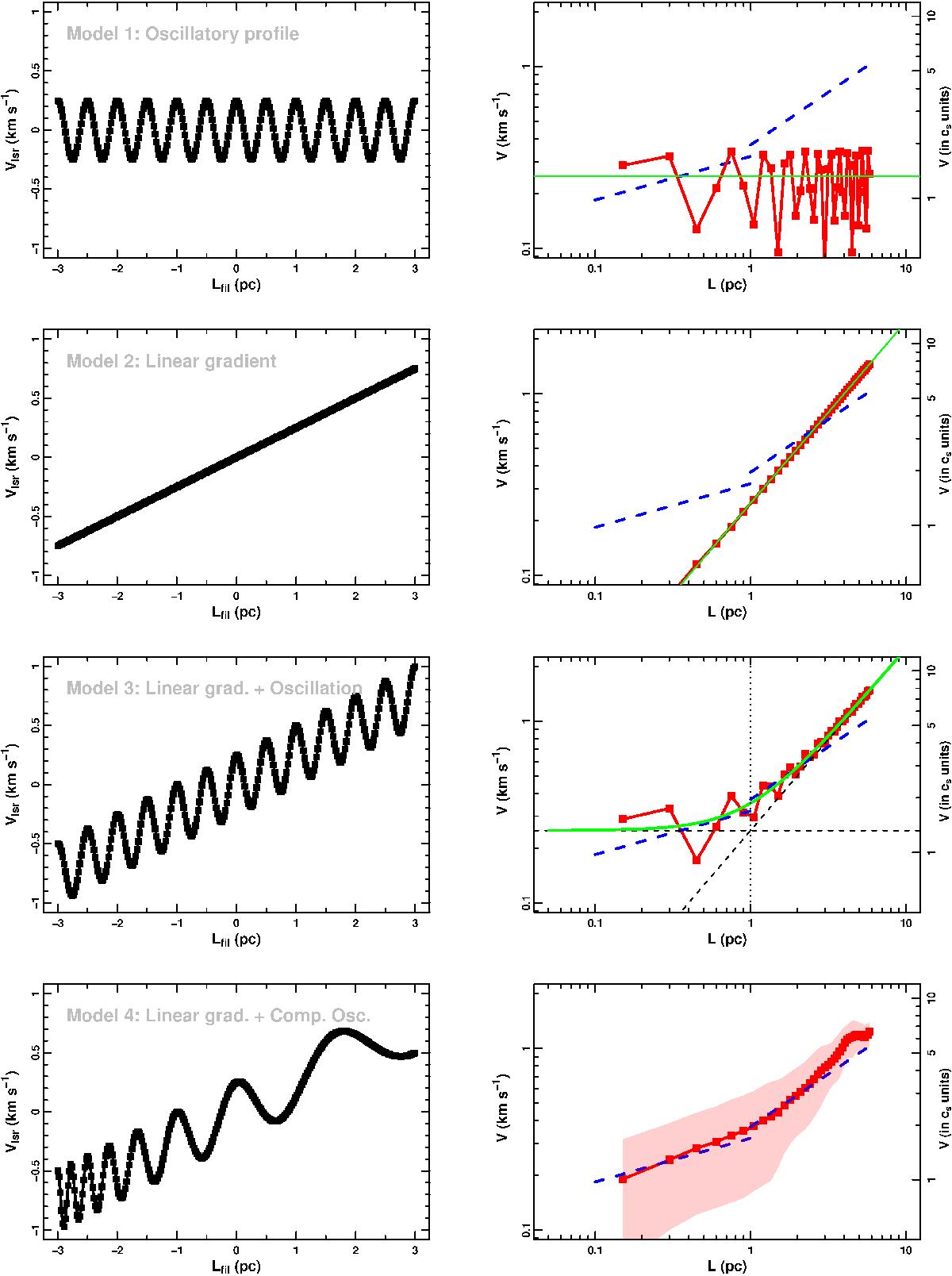
Position velocity diagram (left; black dots) and its corresponding δV( = S₂(L)^{1 / 2}) structure function (right; red dots) for the four 1D filamentary clouds modeled in this work (see also Table 1). From top to bottom: (Model 1) Filament presenting a sinusoidal (i.e. oscillatory) velocity profile with amplitude A = 0.25 km s^-1 and period T = 0.5 pc; (Model 2) filament presenting a longitudinal large-scale velocity gradient with ∇V_lsr = 0.25 km s^-1 pc^-1; (Model 3) filament presenting both a global velocity gradient and an oscillation with similar parameters to Models 1 and 2, respectively; (Model 4) filament presenting a global velocity gradient and a complex oscillatory profile with variable period. The green lines represent the analytical fit of their corresponding structure functions (see Table 2). In the case of Model 3, the vertical dashed line denotes the transitional scale where the global velocity gradient dominates over the local motions, estimated as Λ ~ A/ ∇V_lsr. For all plots, the blue dashed lines indicate the broken power-law dependency observed in Musca (see Fig. 5). Similar to our observations, we note that the completeness limit of δV is restricted to scales ≤3 pc (=L_fil/2) owing to the finite size of our models. The shaded area in the last panel indicates the intrinsic dispersion per bin introduced by the presence of multiple oscillations with different periodicity in Model 4.