| Issue |
A&A
Volume 587, March 2016
|
|
|---|---|---|
| Article Number | A17 | |
| Number of page(s) | 13 | |
| Section | Interstellar and circumstellar matter | |
| DOI | https://doi.org/10.1051/0004-6361/201424725 | |
| Published online | 11 February 2016 | |
Outflow forces in intermediate-mass star formation⋆
1
Leiden Observatory, Leiden University,
Niels Bohrweg 2,
2333 CA
Leiden,
The Netherlands
e-mail:
This email address is being protected from spambots. You need JavaScript enabled to view it.
2
Joint ALMA Offices, Av. Alonso de Cordova 3107,
Vitacura, Santiago,
Chile
3
Max-Planck-Institut für Extraterrestische Physik,
Giessenbachstrasse 2,
85478
Garching,
Germany
4
Harvard-Smithsonian Center for Astrophysics, 60 Garden
Street, Cambridge,
MA
02138,
USA
5
Max-Planck-Institut für Radioastronomie,
Auf dem Hügel 69, 53121
Bonn,
Germany
6
UK Astronomy Technology Center, Royal Observatory
Edinburgh, Blackford
Hill, Edinburgh
EH9 3HJ,
UK
7
Kapteyn Institute, University of Groningen,
Landleven 12, 9747 AD, Groningen, The Netherlands
8
Scuola Normale Superiore, Piazza dei Cavalieri 7,
56126
Pisa,
Italy
9
Netherlands Institute for Space Research, Low Energy Astrophysics
Division, Postbus
800, 9700 AV
Groningen, The
Netherlands
10
Department of Microelectronics, Faculty of Electrical Engineering,
Mathematics and Computer Science, Delft University of Technology,
2628 CD
Delft, The
Netherlands
11
Department of Quantum Nanoscience, Kavli Institute of Nanoscience,
Delft University of Technology, Lorentzweg 1, 2628
CJ, Delft,
The Netherlands
12
Netherlands Institute for Radio Astronomy (ASTRON),
Postbus 2, 7990 AA, Dwingeloo, The Netherlands
13
Astronomical Observatory Institute, Faculty of Physics, A.
Mickiewicz University, Sloneczna
36, 60-286
Poznan,
Poland
14
Jet Propulsion Laboratory, California Institute of
Technology, 4800 Oak Grove
Drive, Pasadena,
CA
91109,
USA
15
Netherlands Research School for Astronomy,
PO Box 9513, 2300 RA
Leiden, The
Netherlands
Received: 30 July 2014
Accepted: 6 July 2015
Abstract
Context. Protostars of intermediate-mass provide a bridge between theories of low- and high-mass star formation. Molecular outflows emerging from such sources can be used to determine the influence of fragmentation and multiplicity on protostellar evolution through the apparent correlation of outflow forces of intermediate-mass protostars with the total luminosity instead of the individual luminosity.
Aims. The aim of this paper is to derive outflow forces from outflows of six intermediate-mass protostellar regions and validate the apparent correlation between total luminosity and outflow force seen in earlier work, as well as remove uncertainties caused by different methodologies.
Methods. By comparing CO 6–5 observations obtained with APEX with non-LTE radiative transfer model predictions, the optical depths, temperatures and densities of the gas of the molecular outflows are derived. Outflow forces, dynamical timescales, and kinetic luminosities are subsequently calculated.
Results. Outflow parameters, including the forces, were derived for all sources. Temperatures in excess of 50 K were found for all flows, in line with recent low-mass results. However, comparison with other studies could not corroborate conclusions from earlier work on intermediate-mass protostars which hypothesized that fragmentation enhances outflow forces in clustered intermediate-mass star formation. Any enhancement in comparison with the classical relation between outflow force and luminosity can be attributed to the use of a higher excitation line and improvement in methods. They are in line with results from low-mass protostars using similar techniques.
Conclusions. The role of fragmentation on outflows is an important ingredient to understand clustered star formation and the link between low- and high-mass star formation. However, detailed information on spatial scales of a few 100 AU, covering all individual members is needed to make the necessary progress.
Key words: circumstellar matter / stars: formation / ISM: jets and outflows / submillimeter: ISM
Data cubes from OTF maps are available at the CDS via anonymous ftp to cdsarc.u-strasbg.fr (130.79.128.5) or via http://cdsarc.u-strasbg.fr/viz-bin/qcat?J/A+A/587/A17
© ESO, 2016
1. Introduction
In the current view of star formation, low-mass (Mstar< 3 M⊙) and high-mass (Mstar> 8 M⊙) star formation are described by different theories. Low-mass theories build on the assumption of singular collapse (Shu et al. 1999), while various high-mass theories focus on clustering and energetic environments (Krumholz et al. 2009; Tan et al. 2014). The poorly studied protostars/protostellar clusters of intermediate-mass (Mstar between 3 and 8 M⊙, Lbol between 30 and 5000 L⊙) provide an ideal test bed for a unified theory of star formation. Such a theory must be able to correctly address the observed level of fragmentation within intermediate-mass protostellar regions, its influence on the observed properties and must simultaneously reproduce predicted populations set by the initial mass function (Bate 2009; Offner et al. 2010; Hansen et al. 2012).
Multiplicity and fragmentation of intermediate-mass protostars is a relatively unexplored area (for the most recent reviews, see Goodwin et al. 2007; Beltrán 2015). Of those studied in detail, very few deeply embedded intermediate-mass protostars are truly isolated single protostars; most are tightly packed clusters of low-mass protostars (e.g., van Kempen et al. 2012) with at times an actual intermediate-mass protostar found near the center (e.g., Fuente et al. 2001). Isolated intermediate-mass protostars are known, but appear to be very rare (L1641 S3 MMS1 is the best candidate, see van Kempen et al. 2012).
Interferometric observations at submillimeter wavelengths are needed to characterize protostellar content of intermediate-mass protostars, down to the very young, heavily embedded protostars. Observations with the required spatial resolution have been obtained for just a handful of cases (e.g., Fuente et al. 2001, 2005, 2012; Teixeira et al. 2007; van Kempen et al. 2012; Carrasco-González et al. 2012). Most studies lack sensitivity and/or spatial resolution to separate emission from individual protostars.
A powerful way to directly probe star formation without time-intensive interferometric observations is through the study of bipolar jets and molecular outflows. The bipolar jet not only allows part of the angular momentum to disperse and gravitational collapse to continue (Arce et al. 2007), it also entrains significant amounts of the surrounding gas, thereby creating the molecular outflow, which is thought to be the main source of mechanical feedback onto the parental cloud (Nakamura & Li 2007). Outflows also facilitate radiative feedback at larger radii, as radiation is able to escape more readily through the lower density outflow cavities than through the protostellar envelopes. These feedback effects dramatically affect fragmentation and mass accretion rates (Offner et al. 2010; Hansen et al. 2012).
Outflows strengths are quantified by the outflow force, FCO. Deriving outflow forces is difficult, requiring sensitive observations of the line wings of molecular tracers across multiple transitions. In practice, CO is used almost exclusively. Recent benchmarking limits variations between methods to less than an order of magnitude (van der Marel et al. 2013).
Outflows emerging from intermediate-mass protostars have been sparsely studied. The most complete study, Beltrán et al. (2008, referred to as B08 from here on) studied outflow forces of a sample of intermediate-mass outflows using a range of methods and data in comparison with detailed observations of one of them, and proposed a correlation between the FCO and total Lbol (see their Sect. 6). This is a change from the relation between FCO and individual luminosity, first identified by Bontemps et al. (1996). Higher mass accretion rates on the driving source, set or influenced by the level of fragmentation, was put forward as the origin of this effect. However, observational constraints and large uncertainties in the sample and the range of methods used to derive outflow forces limited validation of this hyopthesis.
Since the publication of B08, the Atacama Pathfinder Experiment (APEX) and Herschel Space Observatory have enabled regular observations of spectrally resolved mid- and high-J CO emission lines1 of molecular outflows (See van Kempen et al. 2009a,b, 2010; Fich et al. 2010; Yıldız et al. 2010, 2012; Kristensen et al. 2013; San Jose-Garcia et al. 2013). The reliability of outflow force calculations has improved significantly by making use of the larger range of observable CO transitions, the increase in excitation temperatures of these transitions, and the ability to map outflows completely within a reasonable time. One of the main results is the constraint on entrained gas temperatures of individual flows to 50 K or higher (van Kempen et al. 2009b,a), warmer than the classically adopted temperatures of ≈30 K (e.g., Bachiller et al. 2001, and many others), but in line with shock model predictions (Hatchell et al. 1999).
Sample of studied IM protostars.
In this paper, we present new observations using the CHAMP+ instrument mounted on APEX2 of CO and 13CO J = 6–5 emission of outflows emerging from six intermediate-mass protostars, four of which are known to form clusters of low-mass sources. [CI] 2–1 emission is discussed as a complement. The goal of this paper is to validate the relation between outflow force and total luminosity proposed by B08 by making use of the advances of mid-J CO observations and the methodology applied to low-mass protostars developed by this group (van Kempen et al. 2009b,a; Yıldız et al. 2012).
Section 2 describes the observations, source sample and data reduction strategy. Results are given in Sect. 3. Analysis is presented in Sect. 4, while we discuss the importance of the derived physical parameters in Sect. 5. Conclusions and future work are listed in Sect. 6.
2. Observations
The dual-frequency CHAMP+ array receiver (Güsten et al. 2008) mounted on APEX, was used to map the CO J = 6–5 and 13CO J = 6–5 transitions in six intermediate-mass protostars. As a complement, observations of the [CI] 3P2–3P1 were obtained. Observations were carried out between November 2009 and July 2012 using the On-the-fly (OTF) mode. Fast Fourier Transform spectrometer back-ends were attached to each of 7 pixels for each frequency band, providing a spectral resolution better than 0.1 km s-1. Typical system temperatures ranged between 1300 and 2000 K for the 690 GHz receivers and 3500 to 5000 K for the 810 GHz receivers. Maps of at least 2 5 by 25 (CO J = 6–5) and 1′ by 1′ (13CO and [CI]) were obtained. Sensitivities across the maps and sample varied by factors of 2–4 because of the different atmospheric conditions in combination with elevation of the sources. Noise levels increase by a factor of 2 at the map edges (the outer 15′′). The average beam efficiency was derived to be 0.48 for the 690 GHz array and 0.42 for the 800 GHz array. However, there are variations from month to month3. Beam efficiencies for individual scans were taken as close in time as possible to the observation date.
From the system temperature and beam efficiency measurements the total flux uncertainty is assumed to be 20% for the 690 GHz band and 30% for the 800 GHz band.
2.1. Source selection
The targeted sample consisted of all intermediate-mass protostars observable from APEX from the WISH key program on the Herschel Space Telescope4 (van Dishoeck et al. 2011): NGC 2071 (Carrasco-González et al. 2012; van Kempen et al. 2012), L1641 S3 MMS1 (van Kempen et al. 2012), Vela IRS 17 and Vela IRS 19 (Giannini et al. 2005). The sample was completed by Serpens SMM 1 (the most massive low-mass protostar included in WISH, and known to be a single protostar. See van Kempen et al. 2009d; Kristensen et al. 2012) and IRAS 20050+2720 (B08). Table 1 lists all relevant properties (total luminosity, distance, total mass, VLSR and estimated number of members). If conflicting values were reported in existing literature, values presented in van Dishoeck et al. (2011)5 are given.
2.2. Data reduction
During the observations, the raw data-streams were immediately calibrated using the APEX on-line calibrator, assuming an image sideband suppression of 10 dB. 13CO and [CI] observations of L1641 S3 MMS1 had to be reprocessed with the APEX off-line calibration software owing to inaccuracies in the on-line calibration. Afterwards, a full reduction was done using standard routines in the CLASS and GREG packages of GILDAS6. The final data product was transformed into large FITS cubes in main beam temperature scale with a spectral resolution of 0.1 km s-1.
In the [CI] spectrum of Vela IRS 19, an absorption feature at ~0 km s-1 is present. This is caused by large-scale cloud emission at the off position. A spectrum taken at the off position revealed that the absorption is narrow and not affecting emission at the velocities of Vela IRS 19 which is offset by more than 10 km s-1.
3. Results
3.1. Line Profile of central position
Noise levels, integrated and peak intensities at the central position.
Table 2 presents the integrated intensities, peak temperatures and effective noise levels of spectra extracted from the central (0, 0) positions, assumed to be the gravitational centers. We note that not all protostars are covered by the beam at (0, 0). For example, NGC 2071-C (van Kempen et al. 2012) and IRAS 20050−2720 OVRO 2 (B08) are located over 9′′ away from this position. Resulting spectra are shown in Figs. 1 (CO 6–5), 2 (13CO 6–5) and 3 ([CI]).
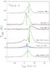 |
Fig. 1 CO 6–5 spectra taken at the central position. The baseline is shown in red. The line profile for L1641 S3 MMS 1 shows an example of the gaussian component fit (overplot in blue). The green lines show the source velocity, also listed in Table 1. |
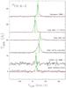 |
Fig. 2 13CO 6–5 spectra taken at the central position. The baseline is shown in red. The green lines show the source velocity, also listed in Table 1. |
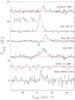 |
Fig. 3 [CI] 3P2–3P1 spectra taken at the central position. The baseline is shown in red. The absorption feature at ~0 km s-1 in Vela IRS 19 is from the off-position but does not affect the main line emission. |
All lines are detected with a signal-to-noise ratio S/N> 10, with the exception of a non-detection of [CI] in L1641 S3 MMS 1. Line profiles of the 12CO 6–5 are dominated by strong line wings, indicative of outflow activity. Absorption features are seen near the source velocities in all sources but their shapes differ from source to source. For NGC 2071, the absorption can be directly associated with large-scale material. The absorption is detected at three distinct velocities coinciding with the velocities of the large-scale CO, 13CO and C18O 3–2 emission profiles (12, 8 and 4 km s-1, see Buckle et al. 2010). As such, it is safe to assume absorptions are caused by cold material in the outer envelope and/or large-scale cloud. The 13CO and [CI] lines are dominated by narrow emission components. Wider components in these lines are only seen for Vela IRS 19 (13CO), NGC 2071 (13CO and [CI]) and Vela IRS 17 ([CI]).
Parameters of the CO 6–5 component fits.
To better analyze the different components, spectra are decomposed by fitting up to three Gaussians to each profile: a “narrow” (FWHM< 4 km s-1), a “medium” (between 4 and 15 km s-1) and a “broad” (>15 km s-1) component. Absorption features are corrected for. This method is similar to the methods used by Kristensen et al. (2010b), Kristensen et al. (2012) and San Jose-Garcia et al. (2013) to deconstruct H2O and high-J CO line profiles. It is possible to identify different outflow components using the medium and broad components and separate them from quiescent components traced by narrow components. Results of the decomposition are presented in Table 3 for CO 6–5 and Table 4 for 13CO 6–5 and [CI] 2–1. A visual example is overplotted in Fig. 1 on the L1641 S3 MMS 1 spectrum.
Parameters of the [CI] 2–1 and 13CO 6–5 component fits.
For CO 6–5, medium components dominate. Only NGC 2071 and L1641 S3 MMS1 show broad components, while narrow emission components were found for Vela IRS19 and Serpens SMM1.
[CI] and 13CO lines decompose into “narrow” and “medium” components, although the widths of the “medium” components are often lower than corresponding 12CO “medium” components. Observed variations in line width of “narrow” components are caused by uncertainties in the fitting routine and the achieved S/N.
3.2. Maps
Figure 4 shows the CO 6–5 emission associated with the molecular outflows in comparison the integrated emission within 2 km s-1 of the VLSR. Outflow emission was measured by integrating between velocities of ±4 to ±20 km s-1 with respect to the source velocity. For the very broad flow emerging from NGC 2071, these cuts were changed to ±10 to ±40 km s-1. If known, positions of (sub)millimeter detected protostars are plotted with white crosses. For the Vela sources, no interferometric (sub)millimeter observations exist to identify individual protostars. Figure 5 shows the emission of 13CO (contours) and [CI] (colors). Map sizes in these lines are typically smaller than the 12CO 6–5.
4. Analysis
4.1. Components at central position
The decomposition of CO 6–5 in Table 3 differs from both the CO 10–9 and 3–2 decompositions in San Jose-Garcia et al. (2013). “Broad” components (>20 km s-1 in width) dominate the CO 10–9, “medium” components the CO 6–5, and “narrow” components the CO 3–2. “Broad” components are detected for CO 3–2, but are relatively weaker than the “narrow” component. Similarly, the two detected “broad” components are weaker than their CO 10–9 counterparts. From a comparison of all three decompositions we conclude that the relative contribution of the “broad” component to the total integrated line flux increases as a function of excitation energy.
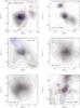 |
Fig. 4 Maps showing the CO J = 6–5 integrated emission in –20 to –4 (blue) and +4 to +20 (red) km s-1 bins to visualize the outflowing gas, overplotted on the integrated emission in a –3 to +3 km s-1 bin (dotted line and grayscale), representing the quiescent emission. All velocities are with respect to the individual source velocity (see Table 1). NGC 2071 was characterized by defining outflow bins at –40 to –10 and +10 to +40 km s-1 instead of the bins above. All contours, including those of the outflowing gas are normalized towards the peak intensity of the quiescent gas component at the central position (Tpeak in Table 2). Levels are in turn given in 10%, 20%, ..., 80%, 90% w.r.t. to this peak intensity. Where known, locations of (sub)millimeter interferometry sources are shown with “×”. |
For sources in our sample where “broad” components are detected in CO 10–9, counterparts in CO 6–5 are likely hidden by the noise; The focus for the CO 6–5 observations above was the size of the maps and not the sensitivity.
13CO emission is dominated by “narrow” emission. As seen in the contours of Fig. 5, it originates in circumstellar envelope in most cases. The exception appears to be IRAS 20050+2720, where 13CO peaks 30′′ southeast of the protostars. For three sources, NGC 2071, Vela IRS 19 and Serpens SMM 1, a “medium” component is detected, but apart from NGC 2071, this component is much weaker than the “narrow” component.
The [CI] emission is dominated by “narrow” emission components. Only NGC 2071 shows emission with a FWHM> 8 km s-1.
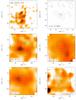 |
Fig. 5 Integrated intensity of 13CO 6–5 (contours) overplotted on the integrated intensity of [CI] (colorscale). Both distributions are normalized to the peak integrated intensity of that particular line. For 13CO the contours are in levels of 10%, 20%, ..., 80%, 90% w.r.t. to this peak intensity, with the lowest contour higher than 3 times the noise level in Table 2. The [CI] emission scales between 3 times the noise level and the highest intensity in the map, which can be found in Table 2. Where known, locations of (sub)millimeter interferometry sources are shown with “×”, except for the Vela sources. |
4.2. Line luminosities
CO line luminosities show a relatively tight relation across the large range of luminosity and mass involved in star formation (Wu et al. 2005, 2010; San Jose-Garcia et al. 2013). The line luminosity relation is defined as 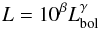 (1)with L the line luminosity (LCO, L[ CI ] or
  ) for CO 6–5, [CI] 3P2-3P1 and 13CO 6–5 respectively.
Figure 6 shows the line luminosities compared to Lbol, including results of CO 6–5 of low-mass protostars from van Kempen et al. (2009b) and van Kempen et al. (2009a). An average value γ of 0.83 ± 0.05 is found, almost identical to 0.84 ± 0.06 of San Jose-Garcia et al. (2013) using Herschel CO 10–9 line observations and spanning the full range in luminosity between 1 and 105Lbol. We note that even with the small sample size, [CI] line luminosities follow the expected correlation between low- and high-mass star formation through total luminosity with a slope of 0.96.
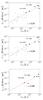 |
Fig. 6 Top: CO 6–5 line luminosity vs. Lbol. Middle: 13CO 6–5 line luminosity vs. Lbol. Bottom: [CI] 3P2–3P1 line luminosity vs. Lbol. Fits to the line luminosities are shown in red, with the slope labeled “γ”. The slopes are within the error bars of San Jose-Garcia et al. (2013). Open symbols are the low-mass sample from Yıldız et al. (2013). No [CI] was reported in Yıldız et al. (2013). The [CI] detections of van Kempen et al. (2009a) are included. |
Derived 12CO 6–5 average optical depths in the center and line wings.
4.3. Optical depths
Table 5 presents three different optical depths derived using the CO 6–5/13CO 6–5 line ratios: at line center (τcenter) and in each of the wings (τblue/τred). A standard 12CO/13CO isotopologue ratio of 65 was used (Wilson & Rood 1994).
Optical depths at line center range from 10 to >25, and are set by foreground absorption. In the wings, optical depths range between <1 and 6.5 with most values between 1 and 3. We note that these are upper limits as a result of the lack of signal at higher velocities in 13CO 6–5. These optical depths are higher than upper limits for low-mass sources (≈1, e.g., NGC 1333: Yıldız et al. 2012, HH46: van Kempen et al. 2009b). Exceptions are IRAS 20050+2720 and NGC 2071, which show optically thin emission in the line wings.
Optical depths at different positions are consistently equal or lower than the optical depths given in Table 5. For convenience, the optical depth for the flows are used for the full maps.
4.4. Outflow properties
Outflow parameters such as kinetic temperatures, densities, outflow forces and kinetic luminosities can be derived by calculating the non-LTE radiative transfer parameters and comparing those with observed line emission. For this sample, the off-line version of the RADEX code (van der Tak et al. 2007) was used provide constraints using ratios of the observed CO 6–5 emission over previously observed transitions of lower excitation (see Table 6). Diagnostical plots for ratios with respect to CO 6–5 are presented in Fig. 7.
 |
Fig. 7 RADEX diagnostic plots of CO 2–1 (top), 3–2 (middle) and 4–3 (bottom). The derived line ratios of the blue flow of Serpens SMM1 are highlighted in red to serve as an illustration for the sub-thermal and thermal excitation scenarios. It is evident that temperatures below 50 K are excluded in all limits as ratios of CO 2–1 and 3–2 over 6–5 do not agree with those of 4–3. |
4.4.1. Temperature and density
Diagnostical plots produced by RADEX as shown in van der Tak et al. (2007) reveal that ratios provide solutions with a degeneracy between temperature and density. To break this degeneracy other molecular tracers are required to independently derive excitation constraints. CO line ratios covering three or more transitions can provide additional information, but are often insufficient to completely solve the degeneracy. However, ratios using the CO 6–5 line emission are able to exclude large areas of the parameter space. For example, temperatures under 50 K are found to be excluded for many outflows (van Kempen et al. 2009b,a; Yıldız et al. 2012). For a more thorough discussion on RADEX solutions concerning CO and including thermal versus sub-thermal excitation, we refer the reader to Yıldız et al. (2012).
To derive the excitation parameters of this sample, RADEX was run in the optically thin limit, adopting the following parameters: a line width of 10 km s-1, a column density of 1012 cm-2, and a background radiation field of 2.73 K.
In turn, the excitation conditions were investigated by considering two scenarios. First, (lower limits to) the temperatures were derived by assuming a density of 105 cm-3. Second, a lower limit for the density is given. This solution is the lowest density at which emission is fully thermalized. In other words, the density given is the lowest density for which the ratio solely depends on temperature (the limits found at the right sides of the diagnostical plots in Fig. 7 where lines are horizontal). These two scenarios were chosen as they likely best reflect the true physical conditions. Results can be found in Table 6.
Temperature limits of 50 K are found for all flows7. These are in agreement with temperature constraints for low-mass protostars (van Kempen et al. 2009b,a; Yıldız et al. 2012) Technically, lower temperatures are not excluded, but require densities >106 cm-3. Spherical envelope modeling restricts such densities to <2000 AU from the central protostar (See Dusty models of Kristensen et al. 2012). Similarly, B08 restricted densities in IRAS 20050+2720 to 1.3–3 × 106 cm-3 at radii <3000 AU. In general, densities at larger radii are significantly lower, with most cloud densities derived to be on the order of 104 cm-3. Compression factors can be invoked to compensate for this change in density (i.e., local density enhancements). However, compression factors of more than three orders of magnitude are required to keep CO emission thermalized along the entire observed flow (>20 000 AU). Molecular tracers such as H2O (Santangelo et al. 2012) or HCO+ (van Kempen et al. 2009b) independently provide density constraints of <106 cm-3, limiting compression factors to two orders of magnitude. As such, the sub-thermal low-n, high-T solution is the preferred solution.
Line wing ratios of 12CO 6–5/J2–J1 and temperature and density estimates using RADEX.
4.4.2. The optically thin limit
Tests were carried out to verify the optically thin assumption used above and the effect higher optical depths would have on the density and temperature derivations. This was done by using significantly higher column densities (1015–1017 cm-2) in the RADEX simulations. These optically thick solutions provide significantly higher constraints on temperature (>200 K instead of >50 K), while the effective ncrit was found to increase, thus increasing the lower limit on the density given in Table 6. Since the derived optical depths for outflowing gas are mostly upper limits, adopting the optically thin RADEX solutions provides us with the most conservative, but likely more realistic, estimate.
4.4.3. Velocity and spatial variations
Line ratios were found to be relatively constant in velocity, with ratio variations typically on the order of 20 to 40%. This is similar to the behavior of CO in flows around HH 46 and NGC 1333 IRAS 2 (Fig. 10 in van Kempen et al. 2009b; Yıldız et al. 2012).
Line ratios at other positions also show little to no significant difference. It can thus be concluded that variations in the excitation mechanisms along the large-scale flows are small.
4.4.4. Mass outflow rate and outflow force
Outflow forces and kinetic luminosities are derived using the H2 column density. Column densities are derived using Eq. (1) of Hogerheijde et al. (1998) using parameters for the CO 6–5 transition, 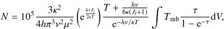 (2)where κ is the Boltzmann constant, h the Planck constant, μ the permanent dipole moment (0.122 Debye for CO), ν the frequency of the transition, Jl the quantum number of the lower rotational state, and
  the integrated line intensity, corrected for optical depth. All quantities are in cgs units, except for the velocity which is in km s-1. The total mass is calculated by summing column densities across the map, assuming a H2/CO ratio of 104.
The outflow force, FCO, is derived using the integrated intensity as a function of velocity, corrected for optical depth and subsequently integrated over the observed area of pixels i and in turn corrected for the inclination. From recent benchmarking, the most reliable method for calculating outflow forces is the “M7” or “separation” method (van der Marel et al. 2013). In this method the dynamical age and force of a flow are considered to be independent quantities. The dynamical age, td is defined as the measured radius, R, divided by Vmax. Using the intensity weighted velocities the outflow force is thus expressed with the following equation: ![Mathematical equation: \begin{eqnarray} F_{\rm CO} = c \times \frac{K (\sum_{i} [ \int T_{\rm mb} \frac{\tau}{1-{\rm e}^{-\tau}} V'{\rm d}V']_i) V_{\rm max}}{R_{\rm lobe}}\cdot \end{eqnarray}](/articles/aa/full_html/2016/03/aa24725-14/aa24725-14-eq80.png) (3)Here c is the inclination correction and K the temperature-dependent correction factor and Rlobe is the radius of the lobe. For more information on this method, see van der Marel et al. (2013). The correction factor is derived from the values of Table 6 of Downes & Cabrit (2007) (see Table 7).
(3)Here c is the inclination correction and K the temperature-dependent correction factor and Rlobe is the radius of the lobe. For more information on this method, see van der Marel et al. (2013). The correction factor is derived from the values of Table 6 of Downes & Cabrit (2007) (see Table 7).
Outflow parameters.
Owing to atmospheric effects, observations at 691 GHz cannot be obtained with a similar S/N as its low-J counterparts within reasonable times. As such, the M7 method was changed on three points w.r.t. van der Marel et al. (2013):
-
1.
Densities derived from line ratios were found to be 104 cm-3 or higher. Therefore, the η = 1 case of Downes & Cabrit (2007) is used instead of the geometric mean of 0.1 and 1 adopted by van der Marel et al. (2013). The latter corresponds to densities below 104 cm-3. As before, these low densities would imply unlikely temperatures of 200 K or higher. Although not excluded, typical envelope models (Kristensen et al. 2012) already have higher densities. In addition, extrapolation of the correction factors from Downes & Cabrit (2007) above 100 K is not reliable.
-
2.
ΔVmax was measured using a 3σ limit, instead of a 1σ limit. Data quality at 690 GHz was found to be insufficient to make a reliable 1σ limit derivation. With the higher system temperatures of the CHAMP+ due to the lower atmospheric transmission at 690 GHz, the effective S/N of the CO 6–5 observations here are a factor of 5 or more lower than for CO 3–2 used by van der Marel et al. (2013). To avoid any potential systematic errors introduced by the data quality but still correctly approach true values for ΔVmax correctly, both td and FCO were corrected with an additional factor of 1.4. This was tested by extrapolating the gaussian fits to Vmax and found to be robust. The correction factor was derived from tests using the appendix of van der Marel et al. (2013) as well as similar tests on data presented here and van Kempen et al. (2009b). td is divided by this correction factor, while FCO is multiplied.
-
3.
No reliable information on individual viewing angles of the outflows with respect to the plane of the sky is available. An average value of 32 degrees for the angle of the outflow with the plane of the sky is adopted. This is the expected mean value for a randomly distributed sample of outflow inclinations.
Table 8 lists the final correction factors used. As a complement to the outflow force, the kinetic luminosity of the flows, Lkin, was calculated using  (4)Table 7 lists the final values for all outflow parameters. Vmax values of both lobes are consistently of similar value, with the exception of the blue side of Vela IRS 19, which is not detected strongly. Its derived parameters are considered lower limits. Dynamical times are a factor of 2 shorter than the average for the low-mass protostar sample (van Kempen et al. 2009c; van der Marel et al. 2013). This may be indicative that no evolved intermediate-mass protostellar cluster was included. Outflow forces are factors of 10 to 300 higher than low-mass protostars (Bontemps et al. 1996). When compared to the results of Duarte-Cabral et al. (2013), the outflow forces found are consistent with the low-end of values for high-mass sources (10-4M⊙ yr-1 km s-1 or higher for luminosities of 100 and higher).
4.4.5. The multiple flows of IRAS 20050+2720
B08 observed IRAS 20050+2720 using a resolution of 3 arcsec. This allows all individual outflows to be identified. It is seen that the observations of interferometers do not resolve out any emission. The total outflowing mass and outflow force co-added for both flows in IRAS 20050+2720 add up to 0.25 M⊙ and 6.4 × 10⁻⁴M⊙ km s-1 yr-1 (B08). Co-added outflow forces from CO 6–5 are less than a factor of 3 higher. With the systematic difference due to the difference in temperature (29 K for B08, 50 K for this study), this factor is well within the assumed inaccuracy of the M7 method (van der Marel et al. 2013).
5. Discussion
5.1. Does fragmentation enhance outflow forces?
Using a large sample of outflows emerging from low-mass protostellar environments, Bontemps et al. (1996, from here on referred to as B96) revealed a relation between the bolometric luminosity of the driving source and the force of its outflow (from here on referred to as the B96 relation). The relation inherently has a relatively large scatter, and the influence of evolutionary effects could not be determined accurately. Since then, many other studies corroborated this relation, and reveals it may apply across the many orders of magnitude in luminosity in star formation, up to and including high-mass star formation (Duarte-Cabral et al. 2013). Figure 8 shows the B96 relation (red line) in comparison with the results obtained here (black filled points) and B08 (white diamonds). Studies of low-mass protostars using CO 6–5 and/or similar methodology to derive outflow forces are included as reference (van Kempen et al. 2009a; van der Marel et al. 2013; Yıldız et al. 2015, gray symbols). For the intermediate-mass flows, the outflow force at first sight correlates with the total Lbol with the B96 relation, similar to the conclusions of B08. The largest deviation from the relation is the NGC 2071 flow, where the outflow force is an order of magnitude higher than expected based on the B96 relation but still well within the observed scatter.
Interestingly enough, the median of the outflow forces in Yıldız et al. (2015) as derived for low-mass sources using CO 6–5 is also statistically significant above the B96 relation. An excess of an order of magnitude for fragmented intermediate-mass sources was identified earlier by B08, although their results were inferred from data with a higher uncertainty on the outflow forces. Direct calculations of gas temperatures, correct derivations of optical depths and a uniform derivation of FCO have improved the reliability of the derived values. The observed excess of B08 can thus neither be corroborated or invalidated. What is more likely is that with the improvements made in observations, the better understanding of the derivation of outflow forces and the access to tracer lines better suited to track entrained outflow material (in this case the CO 6–5), outflow forces are slightly higher than the original B96 relation, although the most important aspect of it, the slope, remains the same.
Correction factors used to multiply the uncorrected value with, from Downes & Cabrit (2007)1 for an inclination i of 30 degrees.
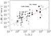 |
Fig. 8 Luminosity versus outflow force of the blue (circle) and red (square) lobes. Black symbols are the derived values for the intermediate-mass protostars, dark gray symbols are values from Yıldız et al. (2015), light gray symbols are values from van Kempen et al. (2009a) and white symbols from van der Marel et al. (2013). All values except the ones from van der Marel et al. (2013) are derived using CO 6–5. White diamonds are the values from B08. The red line represents the relation proposed by Bontemps et al. (1996). |
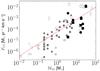 |
Fig. 9 Envelope masses versus outflow force of the blue (circle) and red (square) lobes. Black symbols are the derived values for the intermediate-mass protostars, dark gray symbols are values from Yıldız et al. (2015), light gray symbols are values from van Kempen et al. (2009a) and white symbols from van der Marel et al. (2013). White diamonds are the values from B08. The red line represents the relation proposed by Bontemps et al. (1996). |
Figure 9 compares the FCO and Menv relation of Bontemps et al. (1996) for the same set of samples above with the B96 relation shown as a red line. The correlation between Menv and FCO is clearly visible for intermediate-mass sources and in direct agreement with those derived from low-mass sources. It should be noted that compared to the low-mass sources (shown in white, light gray and dark gray), the scatter for the intermediate-mass sources (shown in black or white diamonds) has increased by a factor of 2. Most likely this enhanced scatter is caused by measurement uncertainties due to intermediate-mass sources being more distant. intermediate-mass sources are a factor of 2 to 5 more distant than typical low-mass sources. From these results, the results of B08 cannot be corroborated. The observed enhancement in outflow forces seen by B08 are reproduced, but are within the scatter of the B96 relation. In addition, the advancement of more accurate observations and differences between them van der Marel et al. (2013) and corresponding constraints can be invoked to explain any changes .
5.2. Neutral carbon
Neutral carbon has long been assumed to be created from interactions of the gas with the interstellar radiation field (ISRF), which produces atomic gas components in a PDR scenario from photo-dissociation of carbon-bearing species (Hollenbach & Tielens 1997), although atomic gas within the outflow cavity surface PDRs could contribute to neutral carbon emission (Hollenbach & Tielens 1997).
Indeed, the observed spatial distribution of the [CI] 3P P1 emission is clearly different from that of CO. In addition, no correlation to the direction and/or strength of the outflow is detected. Figure 5 revealed [CI] emission to be smoothly distributed over the circumcluster envelope, with concentrations at or near the protostellar positions. The only correlation seen for [CI] is in the line luminosity, which reproduces the same slope as derived for CO and 13CO 6–5. This is not surprising as [CI] is clearly expected to be coupled to CO, which scales linearly with luminosity. Whether or not this correlation is evidence for atomic gas emission being correlated with outflow activity itself cannot be confirmed owing to the low number of detections of [CI].
6. Conclusions
This paper presents new spectral line observations of six protostellar clusters of intermediate-mass, with total luminosities ranging from 30 L⊙ to ≈750 L⊙. CO J = 6–5, 13CO J = 6–5 and [CI] spectrally resolved maps were obtained with the CHAMP+ instrument on APEX. Using line decomposition, accurate optical depths and line luminosity relations, densities, temperatures, forces and kinetic luminosities of the molecular outflows were derived and presented. The conclusions can be summed up as follows:
-
The CO 6–5 line profiles are dominated by outflow related emission, but show quiescent emission in the cloud as well.
-
Mid-J CO line luminosities adhere to the correlation between total luminosity and line luminosity identified by San Jose-Garcia et al. (2013) for low- and high-J CO.
-
There is no corroboration of the result presented in Beltrán et al. (2008) that proposed an apparent enhancement in outflow force for fragmented intermediate-mass sources. Although an enhancement of the outflow forces as a function of total bolometric luminosity is seen in comparison with the original B96 relation, this increase can also be attributed to methodology or the improvement in temperature and density derivations due to the inclusion of mid-J CO.
Future work on outflows emerging from protostellar clusters of intermediate-mass require observations down to scales of individual protostars. Properties of individual sources are necessary to draw conclusions about the influence of fragmentation. Although near- and mid-infrared observations have been acquired that can be used (e.g., Spitzer, WISE), (sub)millimeter observations with sufficient spatial and spectral resolution are rare. ALMA is able to routinely do such observations in minutes through several CO transitions, although other interferometers at these wavelengths (SMA, CARMA, IRAM Plateau de Bure and its successor NOEMA) should not be discounted even though their lack of access to mid-J CO lines will limit their effectiveness. The GREAT instrument on SOFIA and in particular the upGREAT array extension of the instrument may spectrally resolve foreground atomic gas from outflowing atomic gas. In combination with ALMA Band 8 and 10, such observations must be used to interpret the [CI] observations.
Throughout this paper low-J CO transitions are defined as having Jup< 4, mid-J CO transition having 4 ≤ Jup ≤ 9 and high-J CO transitions having Jup> 9.
This publication is based on data acquired with the Atacama Pathfinder Experiment (APEX). APEX is a collaboration between the Max-Planck-Institut fur Radioastronomie, the European Southern Observatory, and the Onsala Space Observatory.
See the MPIfR website for more information and distribution of beam efficiency measurements: http://www3.mpifr-bonn.mpg.de/div/submmtech/heterodyne/champplus/
Water In Star-forming regions with Herschel, see http://www.strw.leidenuniv.nl/WISH for more information.
Or B08 in the case on IRAS 20050+2720.
GILDAS is a set of (sub)millimeter radioastronomical applications (either single-dish or interferometer) developed at IRAM, see http://www.iram.fr/IRAMFR/GILDAS
The limit of 10 K for the blue flow of IRAS 20050 was derived with a synthesized beam and is likely suffering from filtered out large-scale emission.
Acknowledgments
T.v.K. is supported by the Allegro ARC node in Leiden and NOVA (Nederlandse Onderzoeksschool voor Astronomie) and NWO (Nederlandse Organisatie voor Wetenschappelijk Onderzoek). R.J.v.W. acknowledges support provided by NASA through the Einstein Postdoctoral grant number PF2-130104 awarded by the Chandra X-ray Center, which is operated by the Smithsonian Astrophysical Observatory for NASA under contract NAS8-03060. A.K. acknowledges support from the Polish National Science Center grant 2013/11/N/ST9/00400 and the Foundation for Polish Science (FNP). Construction of CHAMP+ was a collaboration between the Max-Planck-Institut für Radioastronomie Bonn, Germany; SRON Netherlands Institute for Space Research, Groningen, The Netherlands; The Netherlands Research School for Astronomy (NOVA); and the Kavli Institute of Nanoscience at Delft University of Technology, the Netherlands; with support from the Netherlands Organization for Scientific Research (NWO) grant 600.063.310.10. We thank the APEX staff, in particular the scientists (Per Bergman, Andreas Lundgren, Michael Dumke, Francisco Montenegro and Rodrigo Parra) and operators (Francisco “Pancho” Azagra, Claudio Agurto, Felipe Mac Auliffe, Paulina Venegas and Mauricio Martinez) for their warm welcome over the years.
References
- Arce, H. G., Shepherd, D., Gueth, F., et al. 2007, Protostars and Planets V, 245 [Google Scholar]
- Bachiller, R., Fuente, A., & Tafalla, M. 1995, ApJ, 445, L51 [NASA ADS] [CrossRef] [Google Scholar]
- Bachiller, R., Pérez Gutiérrez, M., Kumar, M. S. N., & Tafalla, M. 2001, A&A, 372, 899 [NASA ADS] [CrossRef] [EDP Sciences] [Google Scholar]
- Bate, M. R. 2009, MNRAS, 392, 1363 [NASA ADS] [CrossRef] [Google Scholar]
- Beltrán, M. T. 2015, Astrophys. Space Sci., 355, 283 [Google Scholar]
- Beltrán, M. T., Estalella, R., Girart, J. M., Ho, P. T. P., & Anglada, G. 2008, A&A, 481, 93 [NASA ADS] [CrossRef] [EDP Sciences] [Google Scholar]
- Bontemps, S., Andre, P., Terebey, S., & Cabrit, S. 1996, A&A, 311, 858 [NASA ADS] [Google Scholar]
- Buckle, J. V., Curtis, E. I., Roberts, J. F., et al. 2010, MNRAS, 401, 204 [NASA ADS] [CrossRef] [Google Scholar]
- Carrasco-González, C., Osorio, M., Anglada, G., et al. 2012, ApJ, 746, 71 [NASA ADS] [CrossRef] [Google Scholar]
- Chini, R., Ward-Thompson, D., Kirk, J. M., et al. 2001, A&A, 369, 155 [NASA ADS] [CrossRef] [EDP Sciences] [Google Scholar]
- Davis, C. J., Matthews, H. E., Ray, T. P., Dent, W. R. F., & Richer, J. S. 1999, MNRAS, 309, 141 [NASA ADS] [CrossRef] [Google Scholar]
- Dionatos, O., Nisini, B., Codella, C., & Giannini, T. 2010, A&A, 523, A29 [NASA ADS] [CrossRef] [EDP Sciences] [Google Scholar]
- Downes, T. P., & Cabrit, S. 2007, ApJ, 471, 873 [Google Scholar]
- Duarte-Cabral, A., Bontemps, S., Motte, F., et al. 2013, A&A, 558, A125 [NASA ADS] [CrossRef] [EDP Sciences] [Google Scholar]
- Elia, D., Massi, F., Strafella, F., et al. 2007, ApJ, 655, 316 [NASA ADS] [CrossRef] [Google Scholar]
- Fich, M., Johnstone, D., van Kempen, T. A., et al. 2010, A&A, 518, L86 [NASA ADS] [CrossRef] [EDP Sciences] [Google Scholar]
- Froebrich, D. 2005, ApJS, 156, 169 [NASA ADS] [CrossRef] [Google Scholar]
- Fuente, A., Neri, R., Martín-Pintado, J., et al. 2001, A&A, 366, 873 [NASA ADS] [CrossRef] [EDP Sciences] [Google Scholar]
- Fuente, A., Neri, R., & Caselli, P. 2005, A&A, 444, 481 [NASA ADS] [CrossRef] [EDP Sciences] [Google Scholar]
- Fuente, A., Caselli, P., McCoey, C., et al. 2012, A&A, 540, A75 [NASA ADS] [CrossRef] [EDP Sciences] [Google Scholar]
- Giannini, T., Massi, F., Podio, L., et al. 2005, A&A, 433, 941 [NASA ADS] [CrossRef] [EDP Sciences] [Google Scholar]
- Goicoechea, J. R., Cernicharo, J., Karska, A., et al. 2012, A&A, 548, A77 [NASA ADS] [CrossRef] [EDP Sciences] [Google Scholar]
- Goodwin, S. P., Kroupa, P., Goodman, A., & Burkert, A. 2007, Protostars and Planets V, 133 [Google Scholar]
- Graves, S. F., Richer, J. S., Buckle, J. V., et al. 2010, MNRAS, 409, 1412 [NASA ADS] [CrossRef] [Google Scholar]
- Güsten, R., Baryshev, A., Bell, A., et al. 2008, in Millimeter and Submillimeter Detectors and Instrumentation for Astronomy IV, eds. W. D. Duncan, W. S. Holland, et al., Proc. Spie, 7020, 25 [Google Scholar]
- Hansen, C. E., Klein, R. I., McKee, C. F., & Fisher, R. T. 2012, ApJ, 747, 22 [NASA ADS] [CrossRef] [Google Scholar]
- Hatchell, J., Fuller, G. A., & Ladd, E. F. 1999, A&A, 344, 687 [NASA ADS] [Google Scholar]
- Hogerheijde, M. R., van Dishoeck, E. F., Blake, G. A., & van Langevelde, H. J. 1998, ApJ, 502, 315 [NASA ADS] [CrossRef] [PubMed] [Google Scholar]
- Hogerheijde, M. R., van Dishoeck, E. F., Salverda, J. M., & Blake, G. A. 1999, ApJ, 513, 350 [NASA ADS] [CrossRef] [PubMed] [Google Scholar]
- Hollenbach, D. J., & Tielens, A. G. G. M. 1997, ARA&A, 35, 179 [NASA ADS] [CrossRef] [Google Scholar]
- Kristensen, L. E., van Dishoeck, E. F., van Kempen, T. A., et al. 2010a, A&A, 516, A57 [NASA ADS] [CrossRef] [EDP Sciences] [Google Scholar]
- Kristensen, L. E., Visser, R., van Dishoeck, E. F., et al. 2010b, A&A, 521, L30 [NASA ADS] [CrossRef] [EDP Sciences] [Google Scholar]
- Kristensen, L. E., van Dishoeck, E. F., Bergin, E. A., et al. 2012, A&A, 542, A8 [NASA ADS] [CrossRef] [EDP Sciences] [Google Scholar]
- Kristensen, L. E., Klaassen, P. D., Mottram, J. C., Schmalzl, M., & Hogerheijde, M. R. 2013, A&A, 549, L6 [NASA ADS] [CrossRef] [EDP Sciences] [Google Scholar]
- Krumholz, M. R., Klein, R. I., McKee, C. F., Offner, S. S. R., & Cunningham, A. J. 2009, Science, 323, 754 [NASA ADS] [CrossRef] [PubMed] [Google Scholar]
- Liseau, R., Lorenzetti, D., Nisini, B., Spinoglio, L., & Moneti, A. 1992, A&A, 265, 577 [NASA ADS] [Google Scholar]
- Morgan, J. A., Schloerb, F. P., Snell, R. L., & Bally, J. 1991, ApJ, 376, 618 [NASA ADS] [CrossRef] [Google Scholar]
- Nakamura, F., & Li, Z.-Y. 2007, ApJ, 662, 395 [NASA ADS] [CrossRef] [Google Scholar]
- Offner, S. S. R., Kratter, K. M., Matzner, C. D., Krumholz, M. R., & Klein, R. I. 2010, ApJ, 725, 1485 [NASA ADS] [CrossRef] [Google Scholar]
- SanJose-Garcia, I., Mottram, J. C., Kristensen, L. E., et al. 2013, A&A, 553, A125 [NASA ADS] [CrossRef] [EDP Sciences] [Google Scholar]
- Santangelo, G., Nisini, B., Giannini, T., et al. 2012, A&A, 538, A45 [NASA ADS] [CrossRef] [EDP Sciences] [Google Scholar]
- Shu, F. H., Allen, A., Shang, H., Ostriker, E. C., & Li, Z.-Y. 1999, in The Origin of Stars and Planetary Systems, eds. C. J. Lada, & N. D. Kylafis (Kluwer Academic Publishers), 193 [Google Scholar]
- Slawson, R. W., & Reed, B. C. 1988, AJ, 96, 988 [NASA ADS] [CrossRef] [Google Scholar]
- Stanke, T., McCaughrean, M. J., & Zinnecker, H. 2000, A&A, 355, 639 [NASA ADS] [Google Scholar]
- Tan, J. C., Beltrán, M. T., Caselli, P., et al. 2014, Protostars and Planets VI, 149 [Google Scholar]
- Teixeira, P. S., Zapata, L. A., & Lada, C. J. 2007, ApJ, 667, L179 [NASA ADS] [CrossRef] [Google Scholar]
- van der Marel, N., Kristensen, L. E., Visser, R., et al. 2013, A&A, 556, A76 [NASA ADS] [CrossRef] [EDP Sciences] [Google Scholar]
- van der Tak, F. F. S., Black, J. H., Schöier, F. L., Jansen, D. J., & van Dishoeck, E. F. 2007, A&A, 468, 627 [NASA ADS] [CrossRef] [EDP Sciences] [Google Scholar]
- van Dishoeck, E. F., Kristensen, L. E., Benz, A. O., et al. 2011, PASP, 123, 138 [NASA ADS] [CrossRef] [Google Scholar]
- van Kempen, T. A., van Dishoeck, E. F., Güsten, R., et al. 2009a, A&A, 507, 1425 [NASA ADS] [CrossRef] [EDP Sciences] [Google Scholar]
- van Kempen, T. A., van Dishoeck, E. F., Güsten, R., et al. 2009b, A&A, 501, 633 [NASA ADS] [CrossRef] [EDP Sciences] [Google Scholar]
- van Kempen, T. A., van Dishoeck, E. F., Hogerheijde, M. R., & Güsten, R. 2009c, A&A, 508, 259 [Google Scholar]
- van Kempen, T. A., Wilner, D., & Gurwell, M. 2009d, ApJ, 706, L22 [NASA ADS] [CrossRef] [Google Scholar]
- van Kempen, T. A., Longmore, S. N., Johnstone, D., Pillai, T., & Fuente, A. 2012, ApJ, 751, 137 [NASA ADS] [CrossRef] [Google Scholar]
- Wang, K., Wu, Y. F., Ran, L., Yu, W. T., & Miller, M. 2009, A&A, 507, 369 [NASA ADS] [CrossRef] [EDP Sciences] [Google Scholar]
- van Kempen, T. A., Kristensen, L. E., Herczeg, G. J., et al. 2010, A&A, 518, L121 [NASA ADS] [CrossRef] [EDP Sciences] [Google Scholar]
- White, G. J., Casali, M. M., & Eiroa, C. 1995, A&A, 298, 594 [NASA ADS] [Google Scholar]
- Wilson, T. L., & Rood, R. 1994, ARA&A, 32, 191 [NASA ADS] [CrossRef] [Google Scholar]
- Wilson, B. A., Dame, T. M., Masheder, M. R. W., & Thaddeus, P. 2005, A&A, 430, 523 [NASA ADS] [CrossRef] [EDP Sciences] [Google Scholar]
- Wouterloot, J. G. A., & Brand, J. 1999, A&AS, 140, 177 [NASA ADS] [CrossRef] [EDP Sciences] [Google Scholar]
- Wu, J., Evans, N. J. I., Gao, Y., et al. 2005, ApJ, 635, L173 [NASA ADS] [CrossRef] [Google Scholar]
- Wu, J., Evans, N. J. I., Shirley, Y. L., & Knez, C. 2010, ApJS, 188, 313 [NASA ADS] [CrossRef] [Google Scholar]
- Yıldız, U. A., van Dishoeck, E. F., Kristensen, L. E., et al. 2010, A&A, 521, A40 [NASA ADS] [CrossRef] [EDP Sciences] [Google Scholar]
- Yıldız, U. A., Kristensen, L. E., van Dishoeck, E. F., et al. 2012, A&A, 542, A86 [NASA ADS] [CrossRef] [EDP Sciences] [Google Scholar]
- Yıldız, U. A., Kristensen, L. E., van Dishoeck, E. F., et al. 2013, A&A, 556, A89 [NASA ADS] [CrossRef] [EDP Sciences] [Google Scholar]
- Yıldız, U. A., Kristensen, L. E., van Dishoeck, E. F., et al. 2015, A&A, 576, A109 [NASA ADS] [CrossRef] [EDP Sciences] [Google Scholar]
- Zhang, Q., Hunter, T. R., Brand, J., et al. 2005, ApJ, 625, 864 [NASA ADS] [CrossRef] [Google Scholar]
All Tables
Line wing ratios of 12CO 6–5/J2–J1 and temperature and density estimates using RADEX.
Correction factors used to multiply the uncorrected value with, from Downes & Cabrit (2007)1 for an inclination i of 30 degrees.
All Figures
|
Fig. 1 CO 6–5 spectra taken at the central position. The baseline is shown in red. The line profile for L1641 S3 MMS 1 shows an example of the gaussian component fit (overplot in blue). The green lines show the source velocity, also listed in Table 1. |
| In the text | |
|
Fig. 2 13CO 6–5 spectra taken at the central position. The baseline is shown in red. The green lines show the source velocity, also listed in Table 1. |
| In the text | |
|
Fig. 3 [CI] 3P2–3P1 spectra taken at the central position. The baseline is shown in red. The absorption feature at ~0 km s-1 in Vela IRS 19 is from the off-position but does not affect the main line emission. |
| In the text | |
|
Fig. 4 Maps showing the CO J = 6–5 integrated emission in –20 to –4 (blue) and +4 to +20 (red) km s-1 bins to visualize the outflowing gas, overplotted on the integrated emission in a –3 to +3 km s-1 bin (dotted line and grayscale), representing the quiescent emission. All velocities are with respect to the individual source velocity (see Table 1). NGC 2071 was characterized by defining outflow bins at –40 to –10 and +10 to +40 km s-1 instead of the bins above. All contours, including those of the outflowing gas are normalized towards the peak intensity of the quiescent gas component at the central position (Tpeak in Table 2). Levels are in turn given in 10%, 20%, ..., 80%, 90% w.r.t. to this peak intensity. Where known, locations of (sub)millimeter interferometry sources are shown with “×”. |
| In the text | |
|
Fig. 5 Integrated intensity of 13CO 6–5 (contours) overplotted on the integrated intensity of [CI] (colorscale). Both distributions are normalized to the peak integrated intensity of that particular line. For 13CO the contours are in levels of 10%, 20%, ..., 80%, 90% w.r.t. to this peak intensity, with the lowest contour higher than 3 times the noise level in Table 2. The [CI] emission scales between 3 times the noise level and the highest intensity in the map, which can be found in Table 2. Where known, locations of (sub)millimeter interferometry sources are shown with “×”, except for the Vela sources. |
| In the text | |
|
Fig. 6 Top: CO 6–5 line luminosity vs. Lbol. Middle: 13CO 6–5 line luminosity vs. Lbol. Bottom: [CI] 3P2–3P1 line luminosity vs. Lbol. Fits to the line luminosities are shown in red, with the slope labeled “γ”. The slopes are within the error bars of San Jose-Garcia et al. (2013). Open symbols are the low-mass sample from Yıldız et al. (2013). No [CI] was reported in Yıldız et al. (2013). The [CI] detections of van Kempen et al. (2009a) are included. |
| In the text | |
|
Fig. 7 RADEX diagnostic plots of CO 2–1 (top), 3–2 (middle) and 4–3 (bottom). The derived line ratios of the blue flow of Serpens SMM1 are highlighted in red to serve as an illustration for the sub-thermal and thermal excitation scenarios. It is evident that temperatures below 50 K are excluded in all limits as ratios of CO 2–1 and 3–2 over 6–5 do not agree with those of 4–3. |
| In the text | |
|
Fig. 8 Luminosity versus outflow force of the blue (circle) and red (square) lobes. Black symbols are the derived values for the intermediate-mass protostars, dark gray symbols are values from Yıldız et al. (2015), light gray symbols are values from van Kempen et al. (2009a) and white symbols from van der Marel et al. (2013). All values except the ones from van der Marel et al. (2013) are derived using CO 6–5. White diamonds are the values from B08. The red line represents the relation proposed by Bontemps et al. (1996). |
| In the text | |
|
Fig. 9 Envelope masses versus outflow force of the blue (circle) and red (square) lobes. Black symbols are the derived values for the intermediate-mass protostars, dark gray symbols are values from Yıldız et al. (2015), light gray symbols are values from van Kempen et al. (2009a) and white symbols from van der Marel et al. (2013). White diamonds are the values from B08. The red line represents the relation proposed by Bontemps et al. (1996). |
| In the text | |
Current usage metrics show cumulative count of Article Views (full-text article views including HTML views, PDF and ePub downloads, according to the available data) and Abstracts Views on Vision4Press platform.
Data correspond to usage on the plateform after 2015. The current usage metrics is available 48-96 hours after online publication and is updated daily on week days.
Initial download of the metrics may take a while.