| Issue |
A&A
Volume 585, January 2016
|
|
|---|---|---|
| Article Number | A99 | |
| Number of page(s) | 53 | |
| Section | Extragalactic astronomy | |
| DOI | https://doi.org/10.1051/0004-6361/201527067 | |
| Published online | 23 December 2015 | |
The DiskMass Survey
X. Radio synthesis imaging of spiral galaxies
1 Instituto de Astrofísica de Canarias (IAC), 38205 La Laguna, Tenerife, Spain
e-mail: This email address is being protected from spambots. You need JavaScript enabled to view it.
2 Departamento de Astrofísica, Universidad de La Laguna, 38206 La Laguna, Tenerife, Spain
3 Kapteyn Astronomical Institute, University of Groningen, PO Box 800, 9700 AV Groningen, The Netherlands
e-mail: This email address is being protected from spambots. You need JavaScript enabled to view it.
4 Department of Astronomy, University of Wisconsin, 475 N. Charter St., Madison, WI 53706, USA
e-mail: This email address is being protected from spambots. You need JavaScript enabled to view it.
5 Institute of Cosmology and Gravitation, Univ. of Portsmouth, Dennis Sciama Building, Burnaby Road, Portsmouth PO1 3FX, UK
6 NRC Herzberg Astronomy and Astrophysics, 5071 West Saanich Road, Victoria, British Columbia, V9E 2E7, Canada
7 Department of Astronomy, University of Maryland, College Park, MD 20742, USA
Received: 27 July 2015
Accepted: 13 October 2015
Abstract
We present results from 21 cm radio synthesis imaging of 28 spiral galaxies from the DiskMass Survey obtained with the VLA, WSRT, and GMRT facilities. We detail the observations and data reduction procedures and present a brief analysis of the radio data. We construct 21 cm continuum images, global Hi emission-line profiles, column-density maps, velocity fields, and position-velocity diagrams. From these we determine star formation rates (SFRs), Hi line widths, total Hi masses, rotation curves, and azimuthally-averaged radial Hi column-density profiles. All galaxies have an Hi disk that extends beyond the readily observable stellar disk, with an average ratio and scatter of RHI/R25 = 1.35 ± 0.22, and a majority of the galaxies appear to have a warped Hi disk. A tight correlation exists between total Hi mass and Hi diameter, with the largest disks having a slightly lower average column density. Galaxies with relatively large Hi disks tend to exhibit an enhanced stellar velocity dispersion at larger radii, suggesting the influence of the gas disk on the stellar dynamics in the outer regions of disk galaxies. We find a striking similarity among the radial Hi surface density profiles, where the average, normalized radial profile of the late-type spirals is described surprisingly well with a Gaussian profile. These results can be used to estimate Hi surface density profiles in galaxies that only have a total Hi flux measurement. We compare our 21 cm radio continuum luminosities with 60 μm luminosities from IRAS observations for a subsample of 15 galaxies and find that these follow a tight radio-infrared relation, with a hint of a deviation from this relation at low luminosities. We also find a strong correlation between the average SFR surface density and the K-band surface brightness of the stellar disk.
Key words: techniques: interferometric / galaxies: spiral / galaxies: kinematics and dynamics / galaxies: fundamental parameters / galaxies: structure
© ESO, 2015
1. Introduction
The observed distribution and kinematics of atomic hydrogen (Hi) gas in galaxies provide important information about their baryonic composition and dynamical state, which is difficult to obtain from optical observations. Generally, Hi gas in disk galaxies has a radial extent greater than the optical disk (e.g., Broeils & Rhee 1997). Consequently, since the rotation speed at large radii is the most important constraint on the total mass of the dark matter halo, Hi observations are critical for decomposing rotation curves into dark and luminous components and establishing the dark matter density profile. In addition, Hi observations are critical for inferring the disk stellar mass density from observed stellar velocity dispersion by providing a direct measurement of the atomic gas component (Westfall et al. 2011b, hereafter Paper IV; Martinsson et al. 2013a, hereafter Paper VII). Furthermore, the atomic gas is the reservoir for the molecular gas and future star formation. These considerations make resolved Hi observations essential for understanding galaxy dynamics, formation, and evolution.
Since the mid 1960s (e.g., Burbidge et al. 1964) it has been known that the rotation curves of disk galaxies often display a non-Keplerian decline or even no decline at all (see the reviews of van der Kruit & Allen 1978; and Faber & Gallagher 1979). The ground-breaking studies of Bosma (1978, 1981a,b) showed that Hi rotation curves, in general, remain flat out to the last measured point, many optical disk scale lengths (hR) from the center. Comparable studies using optical tracers of the ionized gas showed similar results (e.g., Rubin et al. 1978). Extended flat rotation curves were also found by Begeman (1987, 1989) who, with better data and an improved fitting algorithm, demonstrated that the eight galaxies in his sample all showed flat rotation curves. The rotation curve of one of the galaxies in his sample (NGC 3198) even remained flat to within 5 km s-1 out to the last measured point at 11 hR. This generic flatness of extended Hi rotation curves (e.g., Sofue & Rubin 2001) is now commonly interpreted as evidence for the existence of an extended distribution of dark matter that surrounds the exponential stellar disk. The flatness of the rotation curve suggests an R-2 radial decline in the density of the dark matter at radii where the dark matter dominates the total gravitational potential.
One complication in using extended velocity fields for dynamical inference is the presence of warps in the Hi gas distribution. For more than half a century, it has been known that the Hi disk of our own Galaxy is warped in the outer parts (Burke 1957; Kerr 1957), and it later became clear that many spiral galaxies have warps (e.g., Sancisi 1976; Bosma 1981b). We now believe that most Hi disks are warped. Van der Kruit (2007) found that the Hi warp starts at around 1.1 times the truncation radius of the optical disk, and García-Ruiz et al. (2002) even claim that, whenever a galaxy has an extended Hi disk with respect to the stellar disk, it has a warp.
The most common approach to derive a rotation curve in the presence of a warp is to model the observed velocity field with a set of nested tilted rings, allowing the inclination and position angle of the rings to vary with radius. Usually, the position angles of the rings can be readily measured from the velocity field. Begeman (1989) demonstrated that below inclinations of ~40 , a strong degeneracy exists between the inclination and the rotational velocity of a ring, even for symmetric velocity fields with random velocity errors of ~5 km s-1. For low-inclination disks, this degeneracy may yield prohibitively large inclination errors based on the measured Hi velocity fields. However, high-quality optical IFU kinematic data can yield accurate and precise kinematic inclinations for the optical, non-warped disk down to ~15° when using a different approach that models the entire velocity field as a single, inclined disk (Andersen & Bershady 2013). Nonetheless, the presence of non-axisymmetric motions can lead to significant errors at low inclination in all but the most regular velocity fields; solid-body rotation also precludes accurate inclinations derived from kinematics. For the nearly face-on galaxies in this paper, we therefore take advantage of the small scatter in the Tully-Fisher relation (Tully & Fisher 1977; Verheijen 2001) to calculate robust inverse Tully-Fisher inclinations. This is done by comparing the circular velocity of the gas as predicted from the galaxies absolute K-band magnitudes to our measurements of their projected rotation speeds (see Martinsson et al. 2013b, hereafter Paper VI).
The measurement of the azimuthally-averaged radial Hi mass surface density profile (ΣHI(R)) is, on the other hand, much less affected by uncertainties in the inclination. Some studies have noted the similarities in ΣHI(R) among galaxies, especially within the same morphological type (Rogstad & Shostak 1972; Cayatte et al. 1994; Wang et al. 2014). Others point out the diversity in the radial behavior of ΣHI(R) in galaxies with a wide range of global properties (e.g., Verheijen & Sancisi 2001). Swaters et al. (2002) found that the outer part of the ΣHI(R) profile in many late-type dwarf galaxies can be well fitted with an exponential decrease, and it can be argued that spiral galaxies in general should display a similar exponential profile at the outer radii. Here, we parameterize the typical radial behavior of ΣHI(R) and study its dependence on global photometric and kinematic properties of the galaxies.
Our observations also allow us to construct 21 cm continuum images and derive total radio continuum luminosities at 1.4 GHz, which we use to estimate global star formation rates (SFRs). We use these data to investigate the correlation between SFR and other global properties of the galaxies in our sample. We also use literature values from IRAS far-infrared (FIR) fluxes to investigate the FIR-radio correlation (e.g., Condon 1992; Yun et al. 2001).
This paper outlines the data reduction and observational results from 21 cm radio synthesis observations of 28 spiral galaxies from the DiskMass Survey (DMS; Bershady et al. 2010, hereafter Paper I). The main observational goals of the DMS are to obtain rotation curves and velocity dispersion profiles of the stars and ionized gas in a sample of ~40 nearly face-on spiral galaxies, taking advantage of the two custom-built integral field units (IFUs) SparsePak (Bershady et al. 2004, 2005) and PPak (Verheijen et al. 2004; Kelz et al. 2006). The kinematics of the stars and ionized gas were measured with the PPak IFU following Westfall et al. (2011a) and presented in Paper VI. Using these data, together with the results from the Hi observations presented in this paper, we have shown that, in general, spiral galaxies are submaximal (Bershady et al. 2011; Paper VII; Swaters et al. 2014, hereafter Paper IX); at a radius of 2.2 hR, the baryons contribute ≲50% to the total potential in the disk.
Observed galaxies in the reduced Hi sample.
The paper is organized in the following way: Sects. 2 and 3 discuss the sample and the observations carried out with the Westerbork Synthesis Radio Telescope (WSRT)1, the Very Large Array (VLA)2, and the Giant Metrewave Radio Telescope (GMRT)3. In Sect. 4, we describe the data reduction procedures. Observational results such as disk geometry, Hi column-density maps, velocity fields, and rotation curves are described in Sect. 5 and presented in an Atlas (Appendix B). Section 6 presents the Hi properties of the galaxies in the sample, with an investigation of the radial distribution of the Hi gas and an inspection of warps. Section 7 presents results from our measured 21 cm radio continuum fluxes, from which we estimate global SFRs. Finally, Sect. 8 summarizes this work.
2. The reduced H i sample
The complete DMS sample selection procedure has been described in detail in Paper I and an abridged summary is given in Paper VI. All 43 galaxies of the Phase-B sample for which stellar-kinematic measurements were obtained with the IFUs have been imaged at 21 cm using WSRT, VLA, and GMRT. This sample was augmented with UGC 6869 for which stellar-kinematic measurements were obtained with SparsePak during a pilot study. In this paper, the Hi data for 28 of the 44 galaxies are presented; 24 galaxies from the PPak sample presented in Paper VI, and 4 additional galaxies for which stellar-kinematic data were obtained with SparsePak. We refer to the galaxy sample studied here as the “reduced Hi sample”; the galaxies in this sample are listed in Table 1. Properties of these galaxies, such as distances, colors and coordinates, can be found in Paper I and Paper VI. The scope of this paper is limited to a description of the data reduction and a concise analysis of the reduced Hi sample. These radio data products have already been used for analysis in Paper IV, Paper VII, Westfall et al. (2014, hereafter Paper VIII and Paper IX.
3. Observational strategy and configurations
Collecting Hi imaging data for 44 galaxies comprises a substantial observational program. Therefore, in order to collect these data, the observations were distributed over the three largest aperture synthesis imaging arrays that operate at 1.4 GHz, and over multiple observing semesters and cycles. Our strategy was to use the WSRT only for galaxies with a declination (δ) above 30. Because of the east-west configuration of the WSRT antennas, the elliptical synthesized beam of the WSRT is elongated in the north-south direction on the sky, approximately proportional to 1/sin(δ) such that the synthesized beam is ~15″ and circular at the North Celestial Pole, while it is ~15″× 30″ at δ = 30°. At lower declinations, the WSRT beam becomes too large compared to the diameters of the target galaxies. The Y-shape along which the VLA and GMRT antennas are laid out allows for a more or less circular synthesized beam at lower declinations, and these arrays were used to mainly target galaxies at δ< 30°. Of the galaxies for which the Hi data are presented here, 7 were observed with the VLA, 18 with the WSRT, including 3 galaxies previously observed with the VLA, and 6 galaxies were observed with the GMRT. Details of the observational setups depend on the array that was used and are described below. A summary of the observational setups is provided in Tables 1 and 2.
3.1. Observations
Observations with the WSRT were carried out in its maxi-short configuration between July 2007 and November 2008. A total of 234 h was allocated, spread over semesters 07B and 08A with some observations delayed to semester 08B. As an east-west array, the WSRT takes advantage of the Earth’s rotation to sample the UV-plane. Each galaxy was observed during a 12-h track, preceded and followed by observations of a flux calibrator. The excellent phase stability of the WSRT at 1.4 GHz does not require observations of phase calibrators during the 12-h track.
Observations with the VLA were carried out in its C-configuration in September and October 2005. A total of 20 h was allocated, spread over five observing tracks. Each galaxy was observed during 3−5 scans, with each scan lasting ~30 min. Every 30-min scan was bracketed by short observations of a nearby phase calibrator with the same correlator settings. A flux calibrator was observed once during each observing track, with correlator settings that were relevant for the galaxies observed during that track.
Observations with the GMRT were carried out between May 2008 and November 2009. A total of 193 h was allocated, spread over four observing cycles. In each cycle, the allocated time was split up over several tracks that each lasted 10−19 h. During each track, 1−3 galaxies were observed and most galaxies were observed during multiple tracks. Galaxy observations in any given track consist of several scans, each lasting 40−60 min. Similar to the VLA observing strategy, every scan was bracketed by short observations of a nearby phase calibrator with the same correlator settings. A flux calibrator was observed once or twice during each observing track with correlator settings that were relevant for the galaxies observed during that track.
The flux and phase calibrators used for each galaxy are provided in Table 1.
3.2. Telescope configurations and correlator settings
For the WSRT, the longest and shortest baselines in its maxi-short configuration, which provides optimum imaging performance for extended sources within a single 12-h observation, are 2700 and 36 m respectively. This allows for an angular resolution of ~15″ in the east-west direction, while the largest observable structures are ~20′ in size. The longest and shortest baselines of the VLA in its C-configuration are 3400 and 35 m respectively, which allows for an angular resolution of ~13″. The largest observable structures are about 20′. The GMRT consists of 30 dishes in a fixed configuration with 14 dishes located in a central region of about 1 km2 and 16 dishes distributed along three arms of the overall Y-shaped configuration. Its longest baseline is 26 km and the shortest about 100 m without foreshortening, which allows for an angular resolution of ~2″ at 1.4 GHz with the largest observable structures of ~7′. The high angular resolution comes at the expense of Hi column density sensitivity and therefore, during the data reduction, the distribution of baselines was tapered such that the angular resolution of the GMRT observations was similar to the WSRT and VLA observations. In all observations from the three telescopes, the largest observable structures are much larger than our target galaxies (see Table 5).
Configurations of the interferometric observations.
For all galaxies observed with the same telescope, the same correlator settings were used, but the observing frequencies were tuned to match the recession velocity of each galaxy. Observations were carried out in dual-polarization mode to increase the signal-to-noise (S/N) in the unpolarized 21 cm Hi emission line by a factor  . The signal from the correlator was integrated in time intervals of 60, 30, and 16.9 s for the WSRT, VLA and GMRT, respectively, after which the visibilities were recorded. For the WSRT, an observing bandwidth of 10 MHz, or 2110 km s-1 at the rest frequency of 1420.405 MHz, was split into 1024 channels of each 9.77 kHz, or 2.06 km s-1. For the VLA, the observing bandwidth of 3.125 MHz (660 km s-1) was split into 128 channels of each 24.4 kHz (5.15 km s-1), and for the GMRT, the observing bandwidth of 8 MHz (1690 km s-1) was split into 256 channels of each 31.25 kHz (6.60 km s-1). Doppler tracking to heliocentric velocities was enabled for the WSRT and VLA to compensate for the drifting observing frequencies, but not for the GMRT. At these observed frequencies, the full width half maximum (FWHM) of the primary beams of the WSRT, VLA and GMRT are 36′, 30′ and 24′, respectively. Because of the large primary beams, one or more satellites or companion galaxies were often detected within the field of view (FOV) and frequency range covered by the observations.
A summary of the various telescope and correlator settings is provided in Table 2.
4. Data reduction
The reduction and analysis of standard spectral-line aperture synthesis imaging data, such as obtained here, by and large take place in two different domains. Flagging, calibrating, and Fourier transforming the recorded visibilities, including gridding, weighting and tapering, is done in the UV domain. For this purpose we used the Astronomical Image Processing System (AIPS4) software package. Post-imaging reduction and analysis of the data cubes are performed in the image domain with the Groningen Image Processing SYstem (GIPSY5) software package (van der Hulst et al. 1992; Vogelaar & Terlouw 2001). Some details of the data reduction procedures are described below.
4.1. Flagging, calibrating, and Fourier imaging the visibilities
The raw visibilities of a particular galaxy and its associated calibrators were extracted from the recorded data sets of each track, loaded into AIPS, and concatenated if the collected data were distributed over multiple files. Obviously bad data from defunct antennas or data affected by radio frequency interference (RFI) or correlator glitches were flagged. Telescope-based gain, phase, and bandpass corrections were determined using the observed fluxes from the calibrators. Calibrated visibilities of the galaxy scans were closely inspected and additional flags were applied when necessary. Subsequently, the calibrated visibility data of a galaxy were Fourier transformed to the image domain. During the map-making process no “cleaning” or deconvolution was applied to remove the sidelobes of the synthesized beam. For each made data cube, the resulting size of the synthesized beam is listed in Table 1 and indicated in the maps in the Atlas.
Although the calibration procedures in principle are very similar for data from the different arrays, they are rather different in practice. Below, we provide some details of the calibration and imaging procedures separately for the three different arrays.
4.1.1. The WSRT data
The WSRT observations were carried out with Antenna 5 missing from the standard array of 14 antennas as it was equipped with a prototype receiver for the APERTIF system. The collected visibility data were processed and calibrated following standard procedures. Upon loading and concatenating the raw visibility data into AIPS, they were weighted according to the elevation-dependent behavior of the system temperature. Antennas with an anomalous behavior of their system temperature were flagged; three tracks suffered from one dysfunctional antenna, and one track from two dysfunctional antennas. Although the WSRT observations were scheduled as to maximize night-time observing, many galaxies were still partly observed during the day, and solar RFI clearly affected the shortest baseline on several runs. Therefore, in every observation, we removed this RFI by blindly flagging the four shortest baselines (antenna pairs 9A, 9B, AB, and CD) whenever the sun was above the horizon. Before proceeding with the calibration, the visibility amplitudes were visually inspected for both the XX and YY polarizations. Additional data affected by RFI was noted and manually flagged.
A continuum data set was produced by averaging the central 75% of the channels. The expected flux levels of the calibrators 3C 48 and 3C 147 were calculated for the observed frequencies based on the known fluxes and spectral indices for these sources. For calibrator CTD93, which lacks an AIPS model, the Stokes-I flux was set manually to 4.83 Jy, based on the VLA Calibrator Manual6. For calibrator 3C 286, which is approximately 10% linear polarized, the Stokes parameters were set manually to (I,Q,U,V) = (14.65, 0.56, 1.26, 0.00) Jy, taken from the ASTRON homepage7. For every track, antenna-based complex gain and phase corrections were determined for both calibrator scans separately by comparing the observed complex visibilities to the expected fluxes and phases of the calibrators. The corrections were then linearly interpolated in time between the two calibrator scans that bracket the 12-h scan of the galaxy. For each observation, the interpolated gain and phase corrections were transferred from the continuum to the line data set. The shapes of the complex bandpasses of the antennas were determined on the basis of the frequency-dependent complex visibilities for both calibrators separately, and subsequently interpolated in time. The gain-, phase- and bandpass-calibrated visibility data of the galaxies were cleaned from remaining RFI by flagging visibilities with an amplitude above 5σ of the root-mean-square (rms) noise (0.24 ± 0.02 Jy) in the UV data, after subtracting a continuum baseline to the line-free channels. We verified that the 5σ clip level was high enough not to affect the Hi signal itself.
For every galaxy, an initial data cube was made by Fourier transforming the calibrated UV data, including the continuum flux from the galaxy and other sources in the field. From this data cube, the channels that are free of line emission were determined, and these channels were used to fit the continuum baseline for the purpose of flagging RFI as mentioned above. The line-free channels were also averaged to produce a single-channel continuum UV data set for each galaxy. The UV data sets were then Fourier transformed to produce the final line-free continuum image and the Hi+continuum data cube for every galaxy, as well as maps and cubes of the corresponding antenna patterns.
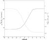 |
Fig. 1 Illustration of the trade-off between angular resolution and column-density sensitivity for different robust weightings of the WSRT visibility data, ranging from uniform to natural weighting. The solid curve indicates the size of the synthesized beam, and the dashed curve shows the 3σ column-density sensitivity in a single channel. |
The WSRT visibilities were given a “Robust = 0” weighting. Figure 1 illustrates the trade-off between angular resolution and column density sensitivity for the WSRT data of UGC 4107. As a function of the “Robust” parameter, it shows the effective angular resolution ( ) as a solid line, and the 3σ Hi column density sensitivity per channel as a dashed line. A value of Robust = −5 corresponds to a uniform weighting of the UV data, yielding the smallest beam (~14″) and the worst column density sensitivity limit (~0.93 ℳ⊙ pc-2). Robust = +5 corresponds to a natural weighting of the UV data, yielding the best column density sensitivity (~0.23 ℳ⊙ pc-2), but the largest beam (~26″) with significant sidelobes. A Robust = 0 weighting provides the best compromise for our purpose, yielding a synthesized beam of 14.3″ × 20.5″ for the case of UGC 4107 at δ = + 49.5°. All data cubes and continuum maps constructed from the WSRT data have a pixel size of 5″ in right ascension and 5″/sin(δ) in declination to properly sample the beam. The channel maps and continuum images have a dimension of 512 × 512 pixels and the antenna patterns a dimension of 1024 × 1024 pixels.
4.1.2. The VLA data
The VLA observations were performed with 4 of the 27 antennas missing from the array as they were being refurbished for the EVLA expansion. The reduction of the VLA data was performed in a way similar to what was described in the previous section, except that antenna-based complex gain corrections and bandpass solutions were derived for each scan of both the flux and the phase calibrators and interpolated in time over the galaxy scans to account for temporal variations.
The calibrated and partially flagged visibilities of an observed galaxy were Fourier transformed into data cubes containing the 21 cm continuum and Hi line emission, as well as cubes with the frequency-dependent antenna patterns. As for the WSRT data, the visibilities were given a Robust = 0 weighting. All data cubes constructed from the VLA data have a pixel size of 4.5′′× 4.5′′ and the same dimensions as the WSRT data cubes.
4.1.3. The GMRT data
The reduction and calibration of the UV data from the GMRT follows the same overall strategy as applied to the WSRT and VLA data, but there are a few notable differences in practice.
First of all, identifying and flagging RFI is much more tedious and time consuming for GMRT data compared to the VLA and WSRT data. This is mainly due to higher levels of RFI at the GMRT site and the larger data volumes generated by the GMRT; the typical data volume per galaxy from the GMRT is ~3 times that from the WSRT and ~14 times that from the VLA. Several remote antennas and long baselines were flagged blindly upfront, motivated by the fact that the highest angular resolution provided by the longest GMRT baselines is not required to obtain a synthesized beam similar to that provided by the VLA and WSRT. Therefore, we flagged a) nine of the outermost antennas that provide the longest baselines; b) baselines longer than 25 kλ between the remaining inner antennas of the array; and c) the nine shortest baselines (<300 m) whenever the sun was above the horizon in order to remove solar RFI. All these antennas and baselines were excluded from the calibration and imaging process. Subsequently, for each track the preliminary-calibrated remaining GMRT visibilities were prepared for visual inspection by arranging them for each polarization in three-dimensional data cubes with baseline number, time and frequency channel as their axes. The visually identified presence of RFI was recorded and flagged manually.
Second, due to steep phase gradients across the 8 MHz bandpass, a continuum data set for determining the gain and phase corrections was made by averaging only ~10 RFI-free channels near the center of the bandpass to avoid effective de-correlation of the signal that would have occurred when the default 75% of the channels would have been averaged.
Third, because the shape of the bandpass of the GMRT is quite stable in time, a single average bandpass was determined for each galaxy by making use of all the scans of the flux and phase calibrators observed for that galaxy.
After some trails and consultation with the staff at the GMRT in Khodad and the NCRA in Pune, the calibrated UV data were Fourier transformed to the image domain with a “Robust = 0” weighting, a Gaussian UV taper with its width at 30% set to 16 kλ in both U and V, and excluding baselines longer than 25 kλ (5.3 km). This yielded angular resolutions that are similar to what was obtained with the VLA and the WSRT as listed in Table 1. All data cubes constructed from the GMRT data have a pixel size of 4′′× 4′′ and the same dimensions as the WSRT and VLA data cubes.
4.2. Post-imaging deconvolution and signal definition
The data cubes produced with AIPS for each galaxy, containing the 21 cm sky signals and corresponding frequency-dependent beam patterns or “dirty” beams (the radio equivalent of a point spread function), were further processed with GIPSY. Before deriving the various data products, the continuum and line emission must be separated and, after defining the regions that contain the continuum and Hi signal in each channel map, the images need to be deconvolved, or “CLEANed”, to remove the sidelobes of the synthesized beams. The post-imaging processing of the data cubes is basically identical for all three arrays and described in detail in the following subsections.
4.2.1. Velocity smoothing
All observations were carried out with a uniform frequency taper which means that the spectral response to an infinitely narrow emission line is a sync function with a FWHM of 1.2 times the width of a frequency channel. Furthermore, strong continuum sources may produce a Gibbs ripple that can affect a large part of the bandpass. To suppress the sidelobes of the sync function and the Gibbs phenomenon, the data cubes were first convolved along the frequency axis with a Hanning smoothing kernel which extends over 3 channels with relative weights of (1/4, 1/2, 1/4). As a consequence, the spectral response function becomes triangular in shape with a FWHM of twice the channel width. At the rest frequency of the Hi line, this corresponds to a velocity resolution of 4.12, 10.3, and 13.4 km s-1 for the WSRT, VLA, and GMRT data, respectively.
To increase the S/N and to obtain a similar velocity resolution as the VLA and GMRT data, the data cubes from the WSRT were smoothed further in velocity to a near-Gaussian response function with a FWHM of 4 channels, or 8.3 km s-1. Subsequently, every other channel in the WSRT data cubes were discarded such that the FWHM of the spectral response function was sampled by 2 channels, reducing the number of channels from 1024 to 512 while each retained channel was doubled in width to 19.5 kHz (4.12 km s-1), and preserved its observed flux density. All operations were performed on both the data cubes and the cubes containing the beam patterns.
4.2.2. Continuum subtraction
From each spectrum in the data cubes, the continuum emission was subtracted using an iterative rejection scheme. A second-order polynomial was fit as a baseline to each spectrum separately and subtracted. Subsequently, the rms noise was calculated in each continuum-subtracted channel map, and pixels above and below 2σ were masked. This mask was transferred to the input data cube and baselines were refitted, ignoring the masked pixels. After subtracting the refitted baselines, the rms was recalculated and the pixel mask was adjusted. This process was repeated until the pixel mask no longer changed significantly. This iterative rejection method maximizes the number of line-free channels in the fitting, while still ensuring that most of the Hi signal was rejected before fitting the final continuum baseline. For the VLA and GMRT data, a continuum map was created by calculating the values of the fitted baselines at the center of the observed bandpass. For the WSRT data, the continuum UV-data sets were already prepared in the UV domain by averaging line-free channels and Fourier transforming that data set to the image domain (Sect. 4.1.1).
For every galaxy, this iterative procedure resulted in a continuum-free data cube that only contains the signal from the Hi-emission line, as well as a line-free image that only contains the continuum flux of the galaxy and other radio sources in the field. In these cubes and images, the line and continuum signal is still convolved with the corresponding beam patterns.
4.2.3. Signal definition and CLEANing
The signal in the continuum images and Hi data cubes was deconvolved with the CLEAN algorithm as developed by Högbom (1974) and implemented in GIPSY. To avoid mistaking noise peaks for signal and to speed up the search for CLEAN components, we defined masks or search areas that contain the continuum and Hi signals. For the Hi data cubes, the shapes of these masks vary from channel to channel as different parts of the rotating Hi disks are seen at different frequencies or recession velocities.
For the continuum images, the masks were made in an iterative way. First, the brightest continuum sources were identified visually and search areas enclosing these sources were created manually. The overall rms noise in the continuum maps was calculated and the maps were CLEANed down to 1σ. This removed the sidelobes of the brightest sources, reduced the rms noise in the maps, and revealed fainter continuum sources for which enclosing search areas were added to the pre-existing ones. The lower rms noise was recalculated and the continuum image was CLEANed again down to 1σ with the updated map containing the search areas. This was repeated until all sidelobes were removed, the noise no longer decreased, and no more fainter sources were revealed. The CLEAN components found within the final set of search areas were restored into the map with a Gaussian beam of the same FWHM and position angle as the dirty beam pattern.
Constructing masks or search areas for the Hi channel maps is more elaborate as the spatially extended Hi signal occurs in many channels and at different locations as a function of frequency. Also, extended emission at lower column densities may disappear below the noise level, which makes it difficult to identify this emission and include it in the search areas. The procedure we adopted was as follows. First, all channel maps in a data cube were CLEANed blindly down to four times the rms noise in a channel map and the detected CLEAN components were restored with a Gaussian beam similar in size and orientation as the dirty beam pattern. This removed most of the sidelobes from the brightest Hi sources, including possible companion galaxies near the velocity extremes of the data cubes. Second, the channel maps were spatially smoothed to a beam that is twice as large as the Gaussian beam with which the CLEAN components were restored for the WSRT and VLA data, and to a 30″ × 30″ beam for the GMRT data. This enhances the S/N of Hi emission at lower column densities. Third, we calculated the rms noise in the spatially smoothed channel maps and selected only those pixels with values above the 2σ level. This resulted in frequency-dependent masks that contain the Hi signal from the galaxies, as well as some >2σ noise peaks. As the final fourth step, we visually inspected the continuation of the search areas in all three dimensions of the data cubes and manually removed all noise peaks. Naturally, there is some risk that the faintest dwarf satellites were misjudged to be noise peaks. Also, the edges of the search areas are affected by noise at the 2σ level and emission from the lowest column density gas, below 2σ in the smoothed channel maps, is still excluded from the search areas.
The channel-dependent search areas based on the smoothed data cubes were used to CLEAN the high-resolution data cubes down to 1σ of the rms noise level. The CLEAN components that were found within the search areas were restored with a Gaussian beam of similar FWHM as the antenna pattern. In the CLEANed channel maps the sidelobes of the beam pattern were fully removed.
It is noteworthy that for 15 of the 28 observed target galaxies we also detected Hi emission from one or more satellites or companion galaxies, but these are not considered in any further analysis. In total, 34 companion galaxies were detected.
5. Data products
In this section, we discuss the primary data products derived from the continuum maps and the Hi data cubes, including flux densities, global Hi lines and their widths and integrated fluxes, Hi maps and radial Hi column density profiles, Hi velocity fields, position-velocity (PV) diagrams, and rotation curves. For every galaxy, the results are collected and presented in the appended Atlas.
The Hi data of UGC 4458 were taken from the WHISP survey (van der Hulst et al. 2001) and have already been presented by Noordermeer et al. (2005). These data were of higher quality than our GMRT observations. For consistency within the set of derived data products, we have taken the data cube that was obtained with the WSRT and re-processed it in the same manner as the other galaxies we observed.
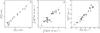 |
Fig. 2 Comparison of our measurements with data from the literature. Left: total 21 cm radio continuum flux densities. Middle: integrated Hi line fluxes. Right: Hi line widths at the 20% level of peak intensity. Solid symbols represent data from the WSRT, open circles from the VLA, and open triangles from the GMRT. The data are listed in Table 3 with references to the literature values. |
5.1. The 21 cm continuum maps and flux densities
The 21 cm continuum flux densities (S21 cm) were measured from the CLEANed continuum maps as presented in the Atlas. Only the flux within the search area of the galaxy used by the CLEAN algorithm was considered. If the galaxy was not clearly detected in radio continuum, S21 cm was calculated in an area that corresponds to the optical disk corrected for the effect of beam smearing. We estimated the formal errors on S21 cm from the rms noise in the maps. All galaxies with a measured S21 cm at least three times higher than the error were considered to have a significant detection. However, four galaxies (UGC 3997, UGC 4380, UGC 4458, UGC 7244) had measured S21 cm lower than three times the error. We have excluded these four galaxies in the following analysis that uses S21 cm measurements. Measured fluxes were corrected for the attenuation of the primary beams, but this is only a minute correction given that the galaxies are relatively small and located near the centers of the FOVs.
The radio continuum maps obtained with the GMRT show strong imaging artefacts from imperfections in the calibration procedure. A proper self-calibration procedure can correct for these effects, but has not been carried out as it is not required for the Hi data in which we are primarily interested8. Because of these artefacts, galaxies observed with the GMRT might have underestimated errors on their S21 cm measurements. We estimate an additional 10% systematic error on S21 cm to account for uncertainties in the flux calibration. The continuum flux densities are presented in Table 3.
The left panel of Fig. 2 shows a comparison of our measured S21 cm for 15 galaxies with literature values reported by the NRAO VLA Sky Survey (NVSS; Condon et al. 1998). We find a reasonable agreement, indicating that our flux calibrations were successful and that we are not suffering from missing short spacings in the UV plane.
Obtained measurements and literature values.
5.2. The global H I profile
The global Hi profile was constructed by calculating the flux density in each channel map within the search area that defines the signal from the galaxy. The error on the flux density measurement was calculated empirically, and we took advantage of the fact that the signal of the galaxy only occupies a small fraction of the data cube. We extracted the smallest data cube that encloses the search areas defining the Hi signal. This small “signal” cube was replicated 27 times in an orthogonal 3 × 3 × 3 configuration within the full data cube, and centered on the target galaxy. Consequently, 26 of the small cubes were centered on line-free areas of the main data cube, modulo the presence of a possible companion galaxy. Subsequently, for every channel in the “signal” cube the flux density was measured within the replicated search area in each of the 26 surrounding “noise” cubes. The error on the flux-density measurement was then calculated as the rms scatter in the 26 flux density measurements from the “noise” cubes. The measured flux densities and their errors were corrected for the minute effect of the primary-beam attenuation. The global Hi profiles are presented in the accompanying Atlas.
5.2.1. Integrated line flux
The integrated Hi line flux ( ) was calculated by summing the primary-beam-corrected flux densities in all channel maps and multiplying it with the channel width (dV) defined to be the velocity width of the central frequency channel. The integrated Hi fluxes are listed in Table 3. The middle panel of Fig. 2 shows a comparison between our integrated Hi fluxes and literature values taken mainly from Bottinelli et al. (1990) and Springob et al. (2005), who collected measurements that were mainly obtained with single-dish telescopes. The correlation between our measurements and the literature values is less strong than for the continuum fluxes; the integrated fluxes reported in the literature tend to be higher than our measurements obtained with the VLA and GMRT arrays (open symbols in Fig. 2) while there is good correspondence with the WSRT measurements (solid symbols).
To investigate whether this offset is caused by a systematic error in the flux calibration of the VLA and GMRT observations we recall the left panel of Fig. 2, demonstrating no systematic offset in the continuum fluxes of the galaxies. To confirm this, we have compared the continuum flux densities of other continuum point sources in the field with those reported by the NVSS. Again, no systematic offset was found. Furthermore, as pointed out earlier, the shortest baselines in our interferometric observations allow us to detect structures that are larger than the dimensions of the targeted galaxies. Therefore, it is unlikely that some of the Hi flux is “resolved out” by the interferometers.
Three of our target galaxies have been observed by both the VLA and WSRT arrays, and for two of those galaxies (UGC 3701 and UGC 11318) the VLA provides a useful integrated Hi flux measurement. These galaxies were also observed with the Green Bank Telescope (GBT) 91 m telescope, with single-dish measurements reported by Springob et al. (2005). There is reasonable correspondence among the integrated fluxes from the VLA, WSRT and GBT measurements: 8.0, 9.2 and 8.4 Jy km s-1 for UGC 3701, and 4.4, 4.7 and 3.1 Jy km s-1 for UGC 11318 for the VLA, WSRT and GBT respectively.
We note that the literature values with which our four VLA measurements are compared in Fig. 2 all come from Springob et al. (2005), who observed these galaxies with the Arecibo telescope. No other galaxies observed by us have literature values from this combination of reference and telescope so there is an exclusive VLA-Arecibo correspondence. We also note that the fluxes measured with Arecibo were corrected by Springob et al. (2005) for pointing offsets and beam-filling effects, following a model that describes the presumed radial extent of the Hi gas in the galaxies. We suspect that these applied beam corrections are systematically too large for the Arecibo observations. Finally, we note that the fluxes as measured by the single-dish observations may be contaminated by contributions from companion galaxies at similar recession velocities as the target galaxies (see Sect. 4.2.3). Indeed, we detect at least one more Hi source in the nearby field at similar recession velocity as the target galaxies for three (UGC 463, UGC 1087, UGC 1635) of the four galaxies observed with the VLA and Arecibo. For UGC 1635, we also detect two more companions, a bit further away from UGC 1635, and just outside the frequency range of that galaxy’s Hi detection. However, these companion galaxies are at a distance of ~10′ from UGC 463 and UGC 1087, and ~5′ from UGC 1635, so should not have contributed enough flux to explain the discrepancy in the flux measurements from the Arecibo telescope, which has a FWHM beam of ~3′.
Given the facts that: a) there is no offset in the continuum fluxes; b) the interferometers can detect the largest structures in our target galaxies; c) there is a reasonable correspondence between the VLA, WSRT and GBT fluxes of 2 galaxies observed by both arrays; and d) significant and uncertain beam corrections were applied to the Arecibo measurements, we conclude that there is no reason to question the integrated Hi fluxes that we have measured.
5.2.2. Line width and rotation speed
The width of the Hi line is traditionally defined to be the full width (in km s-1) between the outer edges of the profile where the flux density is 20% of the maximum observed flux density of the emission line. Variations on this definition include considering the 25% or 50% of the peak flux density or of the mean flux density. In the nominal case of a double-horned profile, the peak flux densities of the two horns may be considered separately as well. Here, we limit ourselves to measuring W20 and W50, the full widths of the profile at 20% or 50% of the absolute peak flux density observed over the entire profile.
We proceed by calculating the velocities at the 20% level ( &
&  ) and the 50% level (
 and
and  ) by linear interpolation between the two channels that are just above and below these thresholds. The widths follow from
  and
and  . The systemic velocities based on the global profiles (
 ) are calculated as
  for both the 20% and 50% levels and then averaged. The error on is taken as half the difference between Vsys,20 and Vsys,50. The measured line widths and their formal errors, as well as the systemic velocities and their errors, are listed in Table 3. The global Hi profiles are presented on the Atlas pages, with W20 indicated by a horizontal dotted line.
The shape of the global Hi profile results from the convolution between the radial distribution of the Hi gas, the rotation curve of the galaxy, and the orientation of the gas disk in terms of its inclination and the possible presence of a warp. Relatively shallow edges of an Hi profile (e.g., UGC 4458 and UGC 8196) hint at the presence of a declining rotation curve or a warp towards an edge-on orientation. The absence of a clear double-horned signature may indicate that the flat part of the rotation curve is not traced by the Hi gas over an extended radial range (e.g., UGC 463) or may be due to a nearly face-on orientation of the disk (UGC 9965 and UGC 11318). In an ideal situation (flat rotation curve, extended Hi disk, no warp), the width of the Hi line is a measure of the maximum rotation speed of the galaxy after application of several corrections to the observed width. Typically, these corrections account for the finite velocity resolution of the instrument, the turbulent motions of the Hi gas, and the inclination of the gas disk.
We correct W20 for instrumental broadening using the expression motivated and provided by Verheijen (2001), ![Mathematical equation: \begin{equation} W_{20}^{\rm R} = W_{20} - 35.8 \left[\sqrt{1+\left( \frac{R}{23.5} \right)^2} -1\right], \label{eq:W20inst} \end{equation}](/articles/aa/full_html/2016/01/aa27067-15/aa27067-15-eq102.png) (1)
(1)
where  is the line width corrected for instrumental broadening, W20 is the observed width, and R is the velocity resolution in km s-1 as listed in Table 3. Given the range of velocity resolutions of our observations, R = 8.3−13.4 km s-1, this correction amounts to a modest9 2−5 km s-1. The right panel of Fig. 2 shows a comparison of our corrected line widths (
 ) with values from the literature, most often obtained from single-dish observations. The correspondence is quite good, keeping in mind that the single-dish observations are often of low S/N while it is not always clear from the literature if and how the correction for instrumental broadening was applied. It should also be noted that global Hi profiles measured with single-dish telescopes may be broadened by Hi emission from satellite galaxies at similar recession velocities.
Subsequently, we correct our profile widths for the turbulent motion of the gas with the expression given by Tully & Fouque (1985)![Mathematical equation: \begin{eqnarray} \left(W_{20}^{R,\rm t}\right)^2 & = & \left(W_{20}^{R}\right)^2 + \left(W_{\rm t,20}\right)^2 \left[1-2{\rm e}^{-\left(\frac{{\rm W}_{20}^{R}}{{\rm W}_{\rm c,20}}\right)^2}\right] \nonumber \\ & & {} - 2 W_{20}^{R} W_{\rm t,20} \left[1-{\rm e}^{-\left(\frac{{\rm W}_{20}^{R}}{{\rm W}_{\rm c,20}}\right)^2} \right] , \label{eq:W20rand} \end{eqnarray}](/articles/aa/full_html/2016/01/aa27067-15/aa27067-15-eq106.png) (2)where the value of the transition parameter is set to Wc,20 = 120 km s-1. The turbulence parameter is set to Wt,20 = 2k20σran. For a purely Gaussian profile k20 = 1.80, but we follow Bottinelli et al. (1983) and adopt k20 = 1.89, accounting for a somewhat narrower core and broader wings than a Gaussian profile. The value of the velocity dispersion is determined by comparing the half-width of the corrected Hi line (
(2)where the value of the transition parameter is set to Wc,20 = 120 km s-1. The turbulence parameter is set to Wt,20 = 2k20σran. For a purely Gaussian profile k20 = 1.80, but we follow Bottinelli et al. (1983) and adopt k20 = 1.89, accounting for a somewhat narrower core and broader wings than a Gaussian profile. The value of the velocity dispersion is determined by comparing the half-width of the corrected Hi line ( /2) with the amplitude of the projected flat part of the rotation curve (Vflatsin(i)) as the average of the [Oiii], Hα, and Hi PV-diagrams (Paper VI). Figure 3 shows the best agreement is found for σran = 10 km s-1, which results in an average difference of +0.4 km s-1 and a scatter of 5.9 km s-1, excluding UGC 4458 which has a declining rotation curve with a flat part much lower than the maximum velocity. The value of σran = 10 km s-1 is higher than observed by O’Brien et al. (2010), who found that most of their gas-rich dwarf systems display velocity dispersions of 6.5−7.5 km s-1, and it is at the high end of the characteristic value of 8−10 km s-1 found by Tamburro et al. (2009) for galaxies more similar to those in our sample. However, compared to Caldú-Primo et al. (2013) who found a median velocity dispersion of 11.9 ± 3.1 km s-1, our value is in the lower end. The correction of the line widths for the turbulent motion of the gas in our galaxies amounts to 18−38 km s-1.
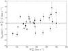 |
Fig. 3 Difference between the weighted-average, projected rotational velocities of the Hα, [Oiii] and Hi PV diagrams and half the corrected widths of the Hi global profiles. The dashed line shows the average difference while the rms scatter is indicated by the two dotted lines. |
Finally, we correct the width of the Hi line for the inclination (iTF; see Sect. 5.4.1) of the galaxy:  (3)The derived
  is indicated as a dashed line in the Atlas rotation-curve panel and can there be compared to the observed rotational velocities.
5.3. The H I column-density map
A total Hi column-density map was made by adding together all channel maps containing Hi emission. Before doing so, the pixels in every channel map that are located outside the search area were set to zero. In this way, we avoid adding noise to areas of the total Hi map from channel maps that do not contain Hi emission from the galaxy at that particular location on the sky. This procedure allows us to obtain a higher S/N, but has the disadvantage that the noise level varies across the total Hi map because a different number of channels were added at each position. The pixel-dependent noise in the Hi map was determined empirically and analogous to the procedure with which the noise in the global Hi profile was determined (Sect. 5.2).
The pixel values of the Hi map were converted to column densities according to ![Mathematical equation: \begin{equation} N_{\rm HI}= 1.823\times 10^{18} \int T_{\rm b}\;{\rm d}V {\rm \;\;\;\;\;\left[atoms\;cm^{-2}\right]} , \label{eq:NHI} \end{equation}](/articles/aa/full_html/2016/01/aa27067-15/aa27067-15-eq119.png) (4)where dV is the velocity range in km s-1 over which the emission line was integrated and Tb is the brightness temperature in Kelvin (K). The conversion from mJy/beam to K for an elliptical Gaussian beam is calculated according to
(4)where dV is the velocity range in km s-1 over which the emission line was integrated and Tb is the brightness temperature in Kelvin (K). The conversion from mJy/beam to K for an elliptical Gaussian beam is calculated according to ![Mathematical equation: \begin{equation} T_{\rm b} = \frac{605.7}{\Theta_x\;\Theta_y}\;S\;\left(\frac{\nu_0}{\nu}\right)^2 \;\;\;\;\; {\rm [K]} , \label{eq:Tb} \end{equation}](/articles/aa/full_html/2016/01/aa27067-15/aa27067-15-eq121.png) (5)where S is the flux density in mJy/beam, Θx and Θy are the major and minor FWHM of the Gaussian beam in arcseconds, ν0 is the rest frequency of the Hi line (1420.40575177 MHz), and ν is the frequency at which the redshifted Hi line is observed. The conversion from [atoms cm-2] to [ℳ⊙ pc-2] is
(5)where S is the flux density in mJy/beam, Θx and Θy are the major and minor FWHM of the Gaussian beam in arcseconds, ν0 is the rest frequency of the Hi line (1420.40575177 MHz), and ν is the frequency at which the redshifted Hi line is observed. The conversion from [atoms cm-2] to [ℳ⊙ pc-2] is ![Mathematical equation: \begin{equation} 1\;\;[\msol\;{\rm pc}^{-2}] = 1.249\times10^{20} \;\; [{\rm atoms}\;{\rm cm}^{-2}] . \label{eq:NHIconv} \end{equation}](/articles/aa/full_html/2016/01/aa27067-15/aa27067-15-eq127.png) (6)The Hi column-density maps can be found in the Atlas with all maps having the same contour levels in terms of ℳ⊙ pc-2.
(6)The Hi column-density maps can be found in the Atlas with all maps having the same contour levels in terms of ℳ⊙ pc-2.
5.4. The observed H I velocity field
The observed velocity field of the rotating Hi disk was created by fitting a single Gaussian to the Hi emission line in the spectrum at every position on the sky. The fitting routine makes use of initial estimates for the amplitude, centroid, and dispersion of the Gaussian function. For each spectrum, the initial estimate for the amplitude is simply the peak flux, while the initial estimates for the centroid and dispersion were calculated as the first and second moment of the spectrum in which pixels outside the search areas were set to zero. The Gaussian fit was accepted if the following four conditions were met: (1) the amplitude of the fitted Gaussian exceeds 2.5 times the rms noise in the spectrum; (2) the centroid of the fitted Gaussian lies within 300 km s-1 of the systemic velocity (from Table 2 in Paper I); (3) the formal error in the centroid is smaller than 5 km s-1; and (4) the velocity dispersion lies in the range 5−100 km s-1. The lower limit in the last condition is motivated by the velocity resolution of the observations, and we expect the velocity dispersion of the Hi gas to be well below the upper limit (e.g., Tamburro et al. 2009).
The observed velocity fields are presented in the Atlas. For presentation purposes only, the values of pixels within the velocity field for which the Gaussian fit failed were calculated by interpolating the values from neighboring pixels, weighted by the Gaussian beam. For subsequent analysis of the kinematics, only pixels with accepted Gaussian fits were considered.
5.4.1. Modeling the H I kinematics
We model the axisymmetric behavior of each observed velocity field with a set of nested, concentric tilted rings following Begeman (1989). Along the major axis, each tilted ring is 10″ wide, or ~2/3 of the size of the synthesized beam, and the radii of the centers of the rings are Rj = 5″ + j × 10″, where j = 0,1, ..., 20. The tilted-ring fitting procedure is carried out in four steps using the ROTCUR program within GIPSY. In these four steps, for each galaxy, we determine: (1) the systemic recession velocity (Vsys); (2) the position angle of the receding kinematic major axis of the gas disk (φ); (3) the inclination of the disk (i); and (4) the rotational velocities (Vrot). We fit Vsys and φ using uniform weighting, while i and Vrot are fit with a cos(φ) weighting. We always use all the data points. The four steps are here described in detail.
Step 1: determine Vsys. We keep the location of the dynamical center of all rings fixed at the morphological center of the galaxy. For the 24 galaxies observed with PPak, we refer to Paper VI for a discussion on how the morphological centers were determined. For the four galaxies observed with SparsePak, we adopt the centers as reported by the Sloan Digital Sky Survey (SDSS)10. The adopted dynamical centers of the galaxies are provided in the Atlas Tables (Appendix B). The inclination of all rings was fixed to be the value derived from the inverse Tully-Fisher relation (i = iTF; see Paper VI). For the four galaxies in the reduced Hi sample that were not discussed in Paper VI, we have calculated their iTF according to the absolute K-band magnitudes (MK) as reported in Paper I. The inferred iTF can be found for each galaxy in the Atlas Table.
After imposing the above restrictions, we fit Vsys, φ and Vrot for each ring such as to reproduce the cosine behavior of the recession velocities as a function of azimuthal angle in the plane of the galaxy. For each galaxy, the radial trend of Vsys is presented in the upper geometry panel on the Atlas page. The Vsys measurement of each galaxy, listed in Table 4, is calculated as the weighted average of all rings and indicated by a horizontal solid line in the Atlas.
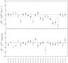 |
Fig. 4 Comparison of results from Hi observations with those from optical PPak observations. The figure shows differences between the systemic velocities (upper panel) and between position angles of the kinematic major axis in the inner regions of the galaxies (lower panel), measured from the Hi velocity fields and those measured with the PPak IFU from [Oiii] and stellar velocity fields (Paper VI). The dashed horizontal lines show the average differences. Solid points correspond to WSRT data, open circles to VLA data, and open triangles to GMRT data. |
In the upper panel of Fig. 4 we compare Vsys derived using our Hi velocity fields ( ) with those derived from the stellar and [Oiii] velocity fields (
 ) obtained with the PPak IFU (see Paper VI). Overall, there is good agreement between the PPak and Hi measurements, with a minor systematic offset of ΔVsys = −2.5 km s-1 or 1/4th of the typical velocity resolution of the Hi observations.
Step 2: determine φ. We now fix Vsys to the value determined in Step 1 for all rings and refit φ and Vrot for each ring. In the observed velocity fields of several galaxies, a twisting of the isovelocity contours in the outer disks often reveals the presence of a warp, and this is generally confirmed by the radial behavior of φ of the fitted tilted rings. The radial trend of φ is presented for every galaxy in the middle geometry panel on the Atlas page. For many galaxies, a φ warp starting outside the FOV of the IFUs (R> 35″) is clearly detected, e.g., for UGC 4036, UGC 6869, and UGC 9965. The representative inner kinematic position angle (φ0) of the gas disk is calculated as the weighted-average position angle of the four inner rings, covering R< 40″, and only including rings containing more than 10 non-blank pixels. Subsequently, we fit a straight line to the measured φ values at R> 40″, forcing φ(R) = φ0 at R = 40″ for continuity. If the slope k of this fitted line is significantly non-zero (| k | more than three times larger than the uncertainty in k) we then allow for the presence of a φ warp in subsequent fitting steps. Otherwise we adopt φ0 to be valid for all outer rings as well. Whenever appropriate, we also adjust the radius at which the φ warp starts, or adjust by eye the radial behavior of the φ warp to better represent the data.
For 14 galaxies in our sample, the shapes of the outer isovelocity contours are best described by introducing a φ warp. The finally adopted radial behavior of the kinematic position angle of the gas disk is indicated by the solid line in the middle geometry panels shown in the Atlas. The position angles representative for the inner gas disks (φ0) are listed in Table 4.
In the lower panel of Fig. 4, we compare the representative position angles derived for the inner Hi velocity fields ( ) with those derived for stellar and [Oiii] velocity fields (
 ) obtained with the PPak IFU (Paper VI). The average difference is
  , with an rms scatter around this mean of
  . UGC 6903 was excluded from the calculation as it has poor PPak data. The systematic offset with a significance of 1.8σ may indicate a small north-south misalignment of the PPak IFU module.
Step 3: attempt to fit i. While keeping the dynamical center, Vsys and φ (with its possible radial dependence) fixed, we fit i and Vrot for each ring. Solutions for these two parameters are highly degenerate for nearly face-on galaxies (Begeman 1989), such that our results are primarily used as a consistency check against the expected iTF values. For each galaxy, the bottom geometry panel in the Atlas shows the best-fit inclination and its formal error for every ring. Indeed, except for a few cases, the formal uncertainties in i are very large. Notable exceptions are UGC 4368 (iTF = 45°), UGC 6869 (iTF = 55°), UGC 6918 (iTF = 38°), and UGC 9837 (iTF = 31°). The first two galaxies are the two most inclined galaxies in the sample, UGC 6918 is in the top-five of the most inclined disks, and the Hi velocity field of UGC 9837 is exceptionally regular and axisymmetric. In all four cases, the average inclinations found from the tilted-ring fits are consistent with the TF-based inclination. Therefore, instead of the results from the tilted-ring fits, we adopt i = iTF for the inner parts of the Hi disks.
An inclination (i) warp with its straight line of nodes is much more difficult to detect than a warp in φ. We have seen, however, that φ warps occur frequently. Given the random orientation of the galaxies in space, i warps should be equally common among our target galaxies. Therefore, to characterize these i warps in our galaxies, we first consider the shape of the deprojected rotation curve under the assumption that i = iTF for the entire disk. Any slope in the rotation curve beyond R = 35″ is removed by adopting a linear i warp that forces the rotation curve to be roughly flat. For ten galaxies in our sample, we judged that introducing such an i warp is warranted. Six of these ten galaxies also display a φ warp.
Step 4: determine Vrot. We fix the dynamical centers and Vsys, as well as the radial behavior of φ and i of the rings as determined in the second and third step. The resulting rotation curves, sampled every 10″ in radius, are indicated for each galaxy by the crosses in the “Rotation Curve” panel, and projected onto the PV diagrams presented in the Atlas.
Properties of the observed Hi velocity fields.
5.4.2. Model and residual velocity fields
Based on the (warped) tilted-ring models derived above, we used the program VELFI in GIPSY to construct model velocity fields. These are presented in the Atlas with the same isovelocity contours as the observed velocity fields. The differences between the observed and modeled velocity fields are shown in the Atlas as residual maps.
When inspecting the observed, modeled, and residual velocity fields, there are several things to keep in mind. First, the model velocity fields are axisymmetric by definition, whereas the observed velocity fields can be significantly asymmetric and affected by non-circular streaming motions. Second, irregular and small-scale structure in the shapes of the isovelocity contours of the observed velocity fields may be caused by the interpolation of observed recession velocities across blank pixels. Third, the model velocity fields are based on inclinations suggested by inverting the Tully-Fisher relation, which may deviate from the formally best-fitting tilted-ring inclinations. Fourth, several observed velocity fields suffer from significant beam-smearing effects which tends to remove curvature from the intrinsic isovelocity contours, making them run more parallel to each other in the inner regions. This results in systematically underestimating the inclination of the tilted rings, worsening the degeneracy between inclination and rotation velocity and increasing the errors on the inclination. An illustrative example is the case of UGC 4555 with its kinematic minor axis aligned along the elongated synthesized beam. The characteristic pattern in its residual velocity field is the tell-tale signature of an inclination mismatch.
5.5. Position-velocity diagram and H I surface density profile
From the cleaned data cubes, we have extracted two-dimensional position-velocity (PV) slices along the inner kinematic major (φ0) and minor (φ0+90) axes of the galaxies, centered on the adopted dynamical centers. These slices do not follow any φ warp and, consequently, the contours of the major-axis PV diagrams do not necessarily indicate the projected rotation curves. The PV diagrams are presented in the Atlas, where the vertical dashed line indicates the position of the dynamical center, while the horizontal dashed line corresponds to Vsys. The small crosses in the PV diagrams indicate the rotation curves as derived in the previous section projected onto the PV diagrams, accounting for possible warps.
The orientation of the tilted rings was also followed when extracting radial Hi surface density profiles from the Hi column density maps. The Hi surface densities were azimuthally averaged in the 10″-wide rings, not only for the entire ring, but also for the receding and approaching sides of the galaxy separately. In the case of a warp, adjacent tilted rings do overlap and the total signal in the overlapping regions was appropriately divided among both rings to conserve the total mass. Finally, the azimuthally-averaged Hi column densities were corrected for the line-of-sight integration through the projected disk, assuming the Hi gas is optically thin along each line of sight. The face-on Hi column-density profiles are also presented on the Atlas pages.
5.6. Correcting rotation curves for beam smearing
Because of beam smearing, the shape of a velocity profile along the line of sight may deviate strongly from a Gaussian, especially in the central region of a galaxy where the velocity gradient across the beam is largest. The velocity profiles are generally skewed by tails towards the systemic velocity, leading to an underestimate of the rotational velocities. This effect also compromises the observed velocity fields in terms of the shapes of the inner isovelocity contours which become less “pinched” towards the dynamical center. For our tilted-ring fitting, we expect beam smearing to yield rotational velocities that may be significantly underestimated in the fourth step of our procedure. This effect can be seen in the PV diagrams for, e.g., UGC 4256 and UGC 9837.
Several methods have been suggested to correct for the effects of beam smearing, e.g., the envelope-tracing method (Sofue & Rubin 2001) which makes use of the terminal velocity in a PV diagram along the major axis, or by correcting the velocity field itself on the basis of local velocity gradients (Begeman 1989). Here, we adopt an interactive variant of the envelope-tracing method following Verheijen & Sancisi (2001). That is, we correct the rotation curves manually by inspecting the PV diagrams along the kinematic major axis. We have considered each cross on the receding and approaching sides of every galaxy and shifted it to the most extreme velocity, while keeping in mind the contour levels, the three-dimensional size of the beam, and the S/N in the data cube. The corrected, but still projected, rotational velocities are indicated in the major-axis PV diagrams, with solid symbols on the receding side and with open symbols on the approaching side of the galaxies. These points are also indicated with the same symbols in the Rotation Curve panels of the Atlas, with a solid line connecting the midpoints. We note that our beam-smearing corrections contribute to kinematic asymmetries in the rotational velocities between the receding and approaching halves of the galaxy.
The errors on the velocities in the beam-corrected rotation curve come from adding the estimated measurement errors (ranging between 1−4 km s-1 on the projected velocities depending on the amplitude of the projected rotation curve, or 4−11 km s-1 on the deprojected velocities depending on the inclination of the galaxy) to half the difference between the measured velocity on the receding and approaching sides. In the few cases where we only have a measurement on one side of the galaxy, we adopt an error based on the average difference at all other radii for which we have measured rotational velocities on both sides.
6. Physical properties of the gas disks
This section summarizes some of the physical properties of the Hi gas disks in our target galaxies such as their absolute and relative Hi masses, diameters, and radial column-density profiles. We also discuss their kinematic properties such as their rotation curves and warps. When considering the following it should be kept in mind that our reduced Hi sample is by no means statistically complete, but merely representative of regular, disk-dominated galaxies. The main purpose of the data collected here is to support the analysis of the baryonic and dark matter mass distributions in the galaxies as presented in Paper VII.
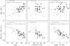 |
Fig. 5 Total and relative Hi masses as a function of MK (left), morphological type (middle), and B−K color (right). The dashed lines are fits to the DMS galaxies (black symbols). The gray symbols shows the galaxies from Verheijen & Sancisi (2001). |
6.1. H I masses
The total Hi mass of each galaxy is derived by calculating ![Mathematical equation: \begin{equation} \mhi\;[\msol] = 2.36\times10^5\; D^2\;[{\rm Mpc}] \int S_{\rm HI}\;[{\rm Jy}]\; {\rm d}V \; [{\rm km~s^{-1}}] , \label{eq:totHI} \end{equation}](/articles/aa/full_html/2016/01/aa27067-15/aa27067-15-eq163.png) (7)where is the integrated Hi line flux listed in Table 3. The Hi masses of our target galaxies, listed in Table 5, range between 1.5 × 10⁹ ℳ⊙ and 2.5 × 10¹⁰ ℳ⊙. The upper panels of Fig. 5 show the total Hi masses against absolute K-band magnitude (MK), morphological type, and B−K color. The total Hi mass correlates well with the total K-band luminosity, but trends with morphological type and color are absent. The most gas-rich galaxies are among the most luminous galaxies that are of type Sb−Scd, but these are not the bluest galaxies in our sample.
(7)where is the integrated Hi line flux listed in Table 3. The Hi masses of our target galaxies, listed in Table 5, range between 1.5 × 10⁹ ℳ⊙ and 2.5 × 10¹⁰ ℳ⊙. The upper panels of Fig. 5 show the total Hi masses against absolute K-band magnitude (MK), morphological type, and B−K color. The total Hi mass correlates well with the total K-band luminosity, but trends with morphological type and color are absent. The most gas-rich galaxies are among the most luminous galaxies that are of type Sb−Scd, but these are not the bluest galaxies in our sample.
When considering the Hi gas content of galaxies per unit luminosity, clear correlations emerge with all three global properties as shown in the lower panels of Fig. 5. The trend with MK is inverted; the most luminous galaxies contain the largest amount of gas, but the lowest relative gas content. Correlations with total luminosity, morphological type, and color are consistent with overall trends along the Hubble sequence and these trends are well known from previous studies (Roberts & Haynes 1994; Broeils & Rhee 1997; Verheijen & Sancisi 2001; Swaters et al. 2002). The linear fits to the correlations are presented in the figure panels, as well as the Spearman rank-order coefficient (rs) of the relations, calculated following Paper VIII. The relative gas-mass fractions in these galaxies were further discussed in Paper VII.
We compare our results with the galaxies in the Ursa Major sample of Verheijen & Sancisi (2001), plotted as gray symbols in Fig. 5. We use the same absolute K-band magnitude of the sun, ℳ⊙ ,K = 3.30 (see Paper IV), for both samples when calculating ℒK. Although the galaxies in Verheijen & Sancisi (2001) have typically much lower total gas masses, as is evident in the top panels, they seem to follow the same relations as the DMS galaxies except for a possible steeper relation between ℳHI/ ℒK and color. However, this difference is not statistically significant.
6.2. Sizes of H I disks
Next, we investigate the sizes (DHI) of the Hi disks, which we define as twice the radius (RHI) at which the azimuthally-averaged Hi column density has dropped to 1 ℳ⊙ pc-2. In the total Hi maps in the Atlas, this column density level is indicated with a thicker contour. In the optical images of the galaxies on the Atlas pages, shown on the same scale as the Hi maps, the inclination and extinction-corrected D25 diameters are indicated by solid ellipses. These D25 values are equal to 2 × R25, the isophotal radius at a blue surface brightness level of 25 mag/arcsec2 as reported by the NASA/IPAC Extragalactic Database11 (NED).
We do not measure RHI from the total Hi maps, but instead from the azimuthally-averaged radial Hi column-density profiles as presented in the Atlas (see Sect. 6.3). The measurement of RHI is affected by beam smearing which results in a somewhat larger radius. We correct for this beam-smearing effect to obtain the corrected Hi radius 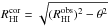 , where
  is the observed radius and θ the beamsize. The correction is only 1−4″ (or 1−6% of ).
The diameters of the gas disks in our target galaxies are 1−2 times the optical diameter D25, or 3−11 times hR. The average ratio and scatter are RHI/R25 = 1.35 ± 0.22, somewhat lower than what has been found in earlier studies (e.g., Broeils & Rhee 1997, who find the ratio 1.7 ± 0.5). Any correlations with the global properties MK, morphological type, and B−K color are absent (see Fig. 4.6 in Martinsson 2011) as noted earlier by Verheijen & Sancisi (2001). Even though the fainter, bluer galaxies of later morphological type in our sample are relatively more gas rich, they do not possess relatively larger Hi disks with respect to their stellar disks.
With these definitions for the optical and Hi diameters, it is clear that the Hi disks extend beyond the optically-recognizable stellar disks, which is consistent with previous work (e.g., Broeils & Rhee 1997; Verheijen & Sancisi 2001; Swaters et al. 2002; Noordermeer et al. 2005). It is noteworthy, however, that the samples studied by Swaters et al. (2002) and Noordermeer et al. (2005) were drawn from the WHISP12 survey which comprised a flux-density-limited parent sample, biased towards more gas-rich galaxies, which tend to have larger gas disks. Volume-limited samples, such as the Ursa Major sample studied by Verheijen & Sancisi (2001), have shown that gas disks are relatively less extended than what has been concluded from flux-density-limited samples.
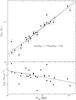 |
Fig. 6 Upper panel: correlation between the total Hi mass (ℳHI) and the beam-corrected diameter of the Hi disk (DHI = 2RHI). The solid line shows the fit to the data while the dashed line represents the correlation found by Verheijen & Sancisi (2001). Lower panel: average Hi mass surface density within RHI versus DHI. The line indicates the expected slope based on the fit in the upper panel. |
6.2.1. Size versus mass and stellar kinematics
Previous studies have revealed a tight correlation between total Hi masses and Hi diameters of the gas disks (Broeils & Rhee 1997; Verheijen & Sancisi 2001; Swaters et al. 2002; Noordermeer et al. 2005). This relation implies an average Hi surface density within the Hi radius that varies only mildly among galaxies. In the upper panel of Fig. 6, we plot the total Hi masses versus the Hi diameters of our target galaxies and we recover a similar tight correlation. The solid line illustrates a linear fit to our data and is described by  (8)where ℳHI is the mass in units of solar masses and DHI the Hi diameter measured in kpc. The dashed line shows the relation found by Verheijen & Sancisi (2001) for galaxies in Ursa Major and the relations are identical within the errors.
The lower panel of Fig. 6 illustrates that the average Hi surface densities within RHI of our 28 target galaxies varies from 1.5 to 5 ℳ⊙ pc-2, with a mean and rms scatter of 3.0 ± 0.8ℳ⊙ pc-2. The fact that the slope in Eq. (8) is not quite 2.0 suggests that the larger Hi disks tend to have slightly lower average Hi surface densities.
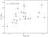 |
Fig. 7 Comparison of the relative kinematic scale lengths of the stellar disks and the relative size of the Hi disks. Galaxies in which the stellar velocity dispersion decreases faster with radius than expected on the basis of the photometric scale length of the stellar disk (hσ/ 2hR< 1), tend to have relatively small Hi disks, and vice versa. |
Although the relative size of the Hi disk does not correlate with galaxy luminosity, color or morphological type, there seems to be a correlation with the ratio of kinematic to photometric scale lengths, as illustrated in Fig. 7. The correlation is weak (rs = 0.39 ± 0.20); however, when dividing the sample in two bins, with 12 galaxies in each bin (only including galaxies in the PPak sample for which we have stellar-kinematic measurements) we find a statistical difference. For galaxies that have smaller Hi disks (RHI< 5.05hR) we find an average ratio hσ/ 2hR = 1.03 ± 0.12, and for galaxies with larger Hi disks (RHI> 5.05hR) we find an average ratio hσ/ 2hR = 1.36 ± 0.19.
For purely exponential disks of constant mass-to-light ratio, scale height and stellar velocity ellipsoid, the stellar velocity dispersion (σ∗) is expected to fall exponentially with radius, with an e-folding length (hσ) that is twice the disk scale length, hσ = 2hR (Paper VI). If hσ/ 2hR> 1, then the stellar disk is kinematically hotter in the outer regions (or the central parts are colder) than what would be expected on the basis of the radial distribution of the stars. As seen in Fig. 7, this seems to be the case in galaxies with extended Hi disks. A possible, but speculative, explanation for this could be that extended gas disks are the result of a continuous or discrete accretion of small gas clouds with their associated stars. Such accretion will likely not be entirely coplanar with the main gas and stellar disks of the accreting galaxy. The accreted gas may quickly settle into the midplane, while the accreted stars continue to circle the galaxy in more inclined orbits, thereby contributing to a higher stellar velocity dispersion in the outer gas-rich disk and a flaring of the stellar disk.
6.3. Radial ΣHI profiles
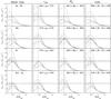 |
Fig. 8 Compilation of all 28 Hi column density profiles, divided in four non-equal bins for each of four global optical properties; morphological type, central disk surface brightness, absolute magnitude, and color. The profiles are scaled in radius by RHI. The horizontal dashed lines are drawn at the sample median |
To investigate whether the Hi column-density profiles (Sect. 5.5) correlate with global properties of the galaxies, we divide the sample of 28 galaxies in 4 groups of ~7 galaxies each along non-uniform intervals of morphological type,  , MK, and color. The results are presented in Fig. 8. Qualitatively, no obvious trends along the columns of Fig. 8 can be discerned. However, galaxies with the highest column densities tend to be of low luminosity and high surface brightness, and galaxies with the lowest column densities tend to be of earlier morphological type, lower surface brightness, higher luminosity, and redder color.
Figure 9 shows the observed, azimuthally-averaged, maximum Hi column density ( ) of every galaxy against its absolute magnitude, color, surface brightness and SFR surface density (ΣSFR) as derived from the radio-continuum flux (Sect. 7). There are only weak correlations in the sense that galaxies with higher peak column densities tend to be bluer with higher star formation densities.
The shapes of the radial Hi column-density profiles of the galaxies all display the same general characteristic; rising from a non-zero value in the center of the galaxy to a maximum value () and then declining following a near-exponential fall-off. This similarity of ΣHI profiles of different galaxies has been noted before (e.g., Cayatte et al. 1994; Broeils & van Woerden 1994). For each galaxy, the values of and DHI = 2RHI are listed in Table 5. It should be noted that the ΣHI profiles considered here have not been corrected for the effects of smearing by the Gaussian beam. The beam smearing slightly lowers the peak column density, raises the central column density, and broadens the profile somewhat. The overall shape, however, will not be altered significantly.
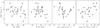 |
Fig. 9 Relations between the maximum, azimuthally-averaged Hi column densities ( |
In the upper panel of Fig. 10, all 28 radial ΣHI profiles are collected and drawn after scaling them in radius with RHI and normalizing their amplitudes by . The solid line shows the average profile shape, calculated after clipping the highest and lowest outlying profiles at every resampled radius. The dashed lines indicate the clipped 1σ rms scatter at each radius. The thinnest lines in the upper panel come from galaxies with earlier morphological types Sa−Sbc and those tend to deviate most from the average profile shape. The crosses in the lower panel of Fig. 10 follow the solid line from the upper panel while the dashed lines are the same and the gray scales indicate intervals of 0.5σ.
Next, we try to parameterize the generic shape of the ΣHI profiles. Given the central depression in the Hi column densities, it is clear that the Hi mass surface density does not follow the typical exponential radial decline of the stars (Freeman 1970). For late-type dwarf galaxies, Swaters et al. (2002) fitted an exponential function to the ΣHI measurements at the outer radii of the profiles with fits that follow the observed profile fairly well in many cases. Wang et al. (2014) analyzed the radial distribution of Hi gas in a sample of 23 galaxies with unusually high Hi content and 19 more “normal” galaxies. They found that an exponential function with a depression in the central parts of the disk, similar to what was proposed by Obreschkow et al. (2009), fit the observed ΣHI profiles well for most of these galaxies.
Attempts to fit an exponential to the outer profiles of the galaxies in our sample were less successful. Instead, we note that the average profile resembles an offset Gaussian function. The solid line in the lower panel of Fig. 10 is a Gaussian fit to the data (crosses), including only the data points above  . This fit is described by
 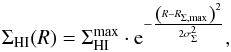 (9)where the peak of the profile occurs at RΣ,max = 0.40RHI and the broadening of the profile is σΣ = 0.36RHI. The fitted profile follows the data surprisingly well, at least out to 1RHI.
From Eq. (9), we derive the radius where the typical Hi mass surface density drops below 50% of the peak to be RΣ,1/2 = 0.81RHI. We measured directly from the profiles the radius at which the azimuthally averaged column density drops below 50% of the peak density. For all 28 galaxies, we found this radius to span 0.49−1.14 RHI with an average value of RΣ,1/2 = 0.80RHI and a standard deviation of 0.12RHI.
We conclude that the ΣHI profiles of our target galaxies are remarkably similar to each other. Possible astrophysical causes for this general shape will be discussed in a forthcoming paper, taking account of the molecular gas component, disk stabilities and SFRs. It is well known that the molecular component closely follows the light distribution with similar scale lengths (Nishiyama et al. 2001; Regan et al. 2001) and the question is whether the atomic and molecular gas components may conspire to produce an exponential decline of the total gas disk with the molecular component filling the central depression of the Hi distribution, as previously discussed by Bigiel & Blitz (2012).
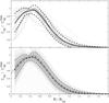 |
Fig. 10 Self-similarity of the Hi column density profiles. Upper panel: all 28 ΣHI profiles scaled in radius and normalized in amplitude. The thinnest lines correspond to the early-type spirals in our sample. The thick black line shows the clipped average profile and the dashed lines indicate the rms scatter at each radius. Lower panel: the crosses follow the thick black line in the upper panel and the dashed lines are identical to the dashed lines in the upper panel. Gray scales indicate steps of 0.5 times the rms scatter. The solid black line is the best-fit Gaussian function following the crosses above (ΣHI/ |

6.4. Kinematics of the gas disks
In this section, we will briefly summarize the kinematics of the gas disks by discussing the shapes of the derived Hi rotation curves and the properties of the warps. In Paper VII, these Hi rotation curves were combined with Hα rotation curves and their combined properties were discussed in more detail.
6.4.1. Rotation curve shapes
The shapes of rotation curves are known to follow some systematic behavior (e.g., Persic et al. 1996). The prototypical rotation curve rises monotonically from the center, roughly consistent with solid-body rotation, then smoothly transitions to a more or less constant rotation speed that persists beyond the radius of the last measured point (e.g., van Albada & Sancisi 1986). This behavior is typical for Sc-type galaxies without a strong bulge component and with rotation speeds in excess of ~120 km s-1. In such systems, the baryons and dark matter conspire to produce a flat rotation curve, and most galaxies in our sample follow this empirical trend.
In galaxies with a significant bulge or very small hR, the rotation curve typically rises very rapidly, reaches a peak, then declines to where the gravitational potential is dominated by the dark matter halo. In our sample, UGC 4458 is a galaxy that displays such a declining rotation curve. Such systems were presented by Casertano & van Gorkom (1991) as examples where the disk-halo conspiracy is lifted and the distribution of baryons clearly leaves a kinematic imprint on the overall shape of the rotation curve. In dwarf galaxies and galaxies of low surface brightness, the rotation curve often continues to rise out to the last measured point (Swaters et al. 2009). Only in dwarf galaxies with very extended Hi disks do the rotation curves reach out far enough into the dark matter halo to display a well-defined flat part (e.g., NGC 3741; Begum et al. 2005). These dwarf galaxies with rotation speeds below ~80 km s-1 are not represented in our sample.
To date, no rotation curve has ever been observed to show a decline in the outer parts that may signify the boundary of the dark matter halo where the density drops faster than ρ ~ R-2. It is also noteworthy that the detailed shape of the inner rotation curve can generally be explained by the distribution of the baryons as traced by the light. An observed rotation curve never rises faster than what would be expected by assuming a maximal disk. Apart from central, super-massive black holes, there is no compelling evidence for dark matter within the inner 2hR if one allows for unconstrained scaling of the baryonic mass. Hence, the central distribution of the total dynamical mass that gives rise to the inner rotation curve seems to follow the distribution of light (e.g., Kent 1986; Sancisi 2004; Swaters et al. 2011; Fraternali et al. 2011; Lelli et al. 2013).
Because of the limited angular resolution of our Hi observations with respect to the sizes of the galaxies, we cannot assess the inner shapes of the rotation curves in detail. And because of the nearly face-on orientation of the galaxies in our sample, inclination warps are often impossible to detect and characterize, which hampers the assessment of the amplitude and slope of the outer Hi rotation curves. Hence, we are not in a good position to investigate the shapes of the rotation curves in detail. With this in mind, we plot all 28 beam-corrected Hi rotation curves together in Fig. 11. The sample is divided in half with black lines indicating galaxies of higher surface brightness ( mag/arcsec2) and gray lines indicating galaxies of lower surface brightness (
 mag/arcsec2). The amplitudes of the rotation curves range from 130 to 270 km s-1 and the maximum radial extent varies from 10−55 kpc. When scaling the rotation curves in radius with hR and in amplitude by the rotational velocity of the flat part Vflat, we see that all rotation curves are fairly self-similar. Notable exceptions are the declining rotation curves of UGC 3140 (black) and UGC 4458 (gray).
6.4.2. Warps
Compared to the readily observable stellar disk, the extended Hi disks more often show morphological and kinematic asymmetries. Furthermore, the fact that a warping of the Hi disk is a common feature was already shown by Sancisi (1976), who found that four out of five observed edge-on systems were warped. Later observations of less inclined galaxies showed features in the Hi velocity fields that were interpreted as warps; an (asymmetric) S-shape of the line of nodes or isovelocity contours that open up or close in on themselves. The method of fitting tilted rings at different radii has been generally used to quantify warps, revealing that many galaxies are warped (e.g., Bosma 1981b). We now think that most Hi disks are warped and García-Ruiz et al. (2002) even claim that all galaxies display warped gas disks provided that they extend well beyond the stellar disk.
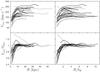 |
Fig. 11 Compilation of all 28 derived rotation curves with different scalings for each panel. The sample of rotation curves is divided in two according to central disk surface brightness: gray curves correspond to galaxies of lower surface brightness ( |


The origin and persistence of warps still presents a puzzle. Many attempts have been made to quantify how often the disks are warped and to explain why they are warped (e.g., Briggs 1990; García-Ruiz et al. 2002; Shen & Sellwood 2006; van der Kruit 2007). There are some indications that the environment may play a role in warping, but the ubiquity of warps suggest that their origin is not simply the result of interaction with the environment. A constant infall of Hi gas, with an angular momentum vector misaligned to that of the inner disk, might explain their formation.
When assessing the frequency and properties of the warps detected in our sample of galaxies, it should be kept in mind that these galaxies were selected to display regular and symmetric morphologies, as well as regular kinematics of their Hα velocity fields (Paper I). Thus, one question to ask is how regular, symmetric, or planar the Hi disks are when the inner Hα disks show well-behaved kinematics. Indeed, if García-Ruiz et al. (2002) are correct, then all our galaxies will display warps as their Hi disks extend beyond the optical disks (Sect. 6.2).
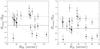 |
Fig. 12 Onset radii of the warps detected in the Hi disks, scaled by RHI (left) and R25 (right). Filled symbols indicate the onset radii of φ warps and open symbols indicate the onset radii of i warps. The solid black and gray lines show the straight average of the i warps and φ warps, respectively. The dashed gray line indicates R = 35″, the edge of the FOV of the PPak IFU. |
A φ warp is relatively easy to detected in nearly face-on galaxies. We have visually inspected three data products presented for each galaxy in the Atlas; 1) the observed Hi velocity field; 2) the PV diagram along the kinematic minor axis; and 3) the results from individual tilted-ring fits at different radii. For many of the galaxies we detect a warp in only one or two of these three data products because of limited S/N, the specific geometry of the warp, or the effects of streaming motions. Nevertheless, 17 out of 28 galaxies show some indication of a φ warp. We deem this warp to be significant in 14 cases and correct accordingly as described in Sect. 5.4.1.
For most of our galaxies the inclination is too unconstrained to be able to detect an i warp, and we have direct indications for an i warp in only a handful of galaxies. For the analysis in this paper, we have assumed that the rotation curves are more or less flat beyond R = 35″, and we enforce a linear i warp in 10 of the galaxies (Sect. 5.4.1). Even though we do not use the inclinations derived from the tilted-ring fits, we note that in several cases there is a trend in these measurements suggesting that there is in fact an i warp somewhat following the enforced warp (see Atlas).
Table 4 lists the radii of the onset of the warps for galaxies that have an adopted φ and/or i warp and Fig. 12 shows these onset radii normalized to the Hi radius (left image) and the optical radius (right image). To be consistent with our measurements of the stellar and ionized gas kinematic obtained with PPak (Paper VI), we have initially chosen to not correct for any warps inside R = 35″. However, for UGC 3997, which has a clear indications of a φ warp starting at ~0.5R25 (see Atlas) well inside the PPak FOV, we make an exception. Van der Kruit (2007) found that when an Hi warp is present, it starts at around 1.1 times the truncation radius of the optical disk (at about 4−5hR). We find that the warps starts at much smaller radii. It should be noted, however, that a φ warp can be mimicked by streaming motions in a strong two-armed spiral disk.
We conclude this section with noting that although we do not detect warps in all galaxies, our result does not contradict García-Ruiz et al. (2002), since, depending on the S/N of the data and the orientation of the disk in the sky, we might not be able to detect the warp.
7. Radio continuum and SFRs
The radio-infrared relation (van der Kruit 1971; Harwit & Pacini 1975; Dickey & Salpeter 1984; de Jong et al. 1985; Condon 1992; Yun et al. 2001; Boyle et al. 2007) is one of the tightest correlations known in astronomy and offers the possibility of deriving SFRs directly from measured radio luminosities, modulo contamination from radio emission due to nuclear activity. The correlation relates the infrared emission from thermal re-radiation of starlight by dust in star-forming regions to the nonthermal synchrotron radiation from relativistic particles accelerated by supernova explosions (Harwit & Pacini 1975; Condon 1992).
In this section we describe how the measured 21 cm continuum flux densities (S21 cm) are converted into intrinsic 21 cm luminosities (L21 cm) and how the SFR is calculated from L21 cm. We investigate correlations between SFR, specific SFR (sSFR), and SFR density (ΣSFR) with other galaxy parameters, and find strongest correlations with the central disk surface brightness of the disk. For all the analysis in this section, we have excluded the four galaxies with <3σ detection in S21 cm (see Sect. 5.1), except for Table 5, which presents (in italic numbers) the SFR for these galaxies calculated from S21 cm as presented in Table 3.
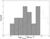 |
Fig. 13 Distribution of 21 cm radio continuum luminosities. The solid histogram displays the distribution of 21 cm radio continuum luminosities of the galaxies in the reduced Hi sample. The dashed histogram shows the distribution for the IRAS galaxies as derived by Yun et al. (2001). |
7.1. 21 cm luminosities
The radio continuum images of our galaxies in the Atlas show that all galaxies with a significant detection display spatially extended emission, except in the case of UGC 8196 where only a central point source is detected. This gives confidence that in most galaxies the 21 cm continuum emission is indeed associated with star formation throughout their disks.
The intrinsic 21 cm radio luminosities are calculated using the relation from Yun et al. (2001)![Mathematical equation: \begin{equation} \log L_{\rm 21 ~cm} \;[{\rm W Hz^{-1}}] = 20.08 + 2\log D\;[{\rm Mpc}] + \log S_{\rm 21~ cm} \;[{\rm Jy}],\label{eq:L21} \end{equation}](/articles/aa/full_html/2016/01/aa27067-15/aa27067-15-eq213.png) (10)where D is the distance, taken from Paper I, and S21 cm is the total flux density listed in Table 3. The histogram in Fig. 13 shows the distribution of 21 cm luminosities of the galaxies in our sample, spanning a factor 50 in luminosity and ranging from 5 × 10²⁰ to 2.5 × 10²² W Hz-1. The dashed line shows the distribution found by Yun et al. (2001) for the IRAS 2Jy sample, with counts normalized to our sample. The differences in the distributions come from selection effects, where the IRAS 2Jy sample is biased towards galaxies with higher luminosities, while our sample is biased towards galaxies with quiescent disks. This figure illustrates that our galaxies are not among the most vigorous star forming systems, as expected.
(10)where D is the distance, taken from Paper I, and S21 cm is the total flux density listed in Table 3. The histogram in Fig. 13 shows the distribution of 21 cm luminosities of the galaxies in our sample, spanning a factor 50 in luminosity and ranging from 5 × 10²⁰ to 2.5 × 10²² W Hz-1. The dashed line shows the distribution found by Yun et al. (2001) for the IRAS 2Jy sample, with counts normalized to our sample. The differences in the distributions come from selection effects, where the IRAS 2Jy sample is biased towards galaxies with higher luminosities, while our sample is biased towards galaxies with quiescent disks. This figure illustrates that our galaxies are not among the most vigorous star forming systems, as expected.
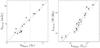 |
Fig. 14 Radio-infrared correlation of 15 galaxies in the reduced Hi sample detected by IRAS at 60 μm. Left: correlation between flux densities. The solid line indicates the simple relation S21cm = 0.01S60 μm. The dashed line shows the correlation found by Yun et al. (2001) for the IRAS 2 Jy sample. The vertical line indicates their lower flux-density limit of 2 Jy. Right: correlation between intrinsic radio and infrared luminosities. |
7.2. The radio-FIR correlation
As mentioned above, there is a tight correlation between far-infrared (FIR) and radio luminosities. Here we investigate this correlation for the galaxies in our sample, using flux densities at 60 μm from IRAS observations (Neugebauer et al. 1984; Moshir et al. 1990). This is done for the 15 galaxies in our sample with reported detections at 60 μm in the IRAS Faint Source Catalogue. Figure 14 shows the correlation between our measured continuum fluxes (S21 cm) and the IRAS fluxes at 60 μm (S60 μm), as well as the correlation when converting fluxes to luminosities (L21 cm and L60 μm). The galaxies in our sample follow the relation described by Yun et al. (2001, dashed gray line), but have the tendency to lie slightly above that relation, being somewhat overluminous in the radio continuum flux. The solid black line shows the simple relation 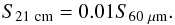 (11)For lower intrinsic luminosities of L60 μm ≤ 109 ℒ⊙, Condon et al. (1991) and Yun et al. (2001) found a deviation from this linear behavior in the sense that fainter galaxies become underluminous in their radio emission compared to their FIR emission. We may see something similar for our galaxies, with a few galaxies around L60 μm = 3 × 10⁹ℒ⊙ having L21 cm lower than expected from the linear relation. However, these are only a handful galaxies, and the two faintest galaxies (with large errors) are instead above the relation. Given the small number of galaxies in our sample, this offset is not statistically significant.
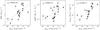 |
Fig. 15 Relations between disk surface brightness ( |
7.3. Star formation rates
To convert the radio luminosities to SFRs, we use the calibration defined by Yun et al. (2001), ![Mathematical equation: \begin{equation} {\it SFR}\; \left[{\msol\; \rm yr^{-1}}\right] = \left(5.9 \pm 1.8\right) \times 10^{-22}\; L_{\rm 21 cm}\; \left[\rm W\; Hz^{-1}\right] . \label{eq:SFR} \end{equation}](/articles/aa/full_html/2016/01/aa27067-15/aa27067-15-eq227.png) (12)The derived SFRs range from 0.16−15 ℳ⊙/yr (Table 5). Recall that in principle there might be contamination from active galactic nuclear (AGN) emission in several galaxies, but we do not try to correct for that here. Based on the width and intensity of the [Oiii] emission line in the central fiber of the PPak observations (Paper VI), UGC 1908, UGC 4036, UGC 6918, UGC 8196, and UGC 11318 may harbor an AGN. Among the 15 galaxies for which we have IRAS measurements, any strong contribution from AGN-related radio emission would show up as a radio-excess object in Fig. 14. There are no galaxies that show a major excess of radio emission, with the possible exception of UGC 11318 at S21 cm = 22 mJy. The continuum map of this galaxy, however, does not show a strong central radio point source. Our results are consistent with the radio-FIR correlation of Yun et al. (2001), who found that only 1.3% of the galaxies they selected had an excess of radio emission.
(12)The derived SFRs range from 0.16−15 ℳ⊙/yr (Table 5). Recall that in principle there might be contamination from active galactic nuclear (AGN) emission in several galaxies, but we do not try to correct for that here. Based on the width and intensity of the [Oiii] emission line in the central fiber of the PPak observations (Paper VI), UGC 1908, UGC 4036, UGC 6918, UGC 8196, and UGC 11318 may harbor an AGN. Among the 15 galaxies for which we have IRAS measurements, any strong contribution from AGN-related radio emission would show up as a radio-excess object in Fig. 14. There are no galaxies that show a major excess of radio emission, with the possible exception of UGC 11318 at S21 cm = 22 mJy. The continuum map of this galaxy, however, does not show a strong central radio point source. Our results are consistent with the radio-FIR correlation of Yun et al. (2001), who found that only 1.3% of the galaxies they selected had an excess of radio emission.
7.3.1. Correlations with other global properties
Apart from the total SFR, we also calculate the SFR per unit K-band luminosity, or specific SFR (sSFR = SFR/ ℒK), and the SFR per unit surface area within R25, or SFR surface density (ΣSFR). We investigate any correlations between these star formation properties with the global photometric properties MK, B−K color, and . We find a clear correlation between SFR and MK, in the sense that more luminous galaxies have a higher SFR. This is not surprising as more massive galaxies will have higher absolute star formation. There is also a trend that redder galaxies tend to have a higher SFR, since the most massive galaxies also tend to be redder. However, when looking at the relative SFR (sSFR or ΣSFR) the correlations disappear (see Fig. 4.16 in Martinsson 2011). Interestingly though, there are strong correlations between all star formation properties and the disk surface brightness (Fig. 15). Galaxies with high surface brightness have both higher absolute and relative star formation, where the strongest correlation is between ΣSFR and . The Spearman rank-order coefficients (rs; calculated following Paper VIII) are presented in the panels of Fig. 15. The linear fits to the correlations, indicated by dashed lines, are given by
![Mathematical equation: \begin{eqnarray} &&\log ({\it SFR}) = 0.208 - 0.409 \left[\mu_{0,K}^{i} - 18\right] , \\ &&\log (s{\it SFR}) = -10.6 - 0.225 \left[\mu_{0,K}^{i} - 18\right] , \\ &&\log (\Sigma_{\rm SFR}) = -2.72 - 0.415 \left[\mu_{0,K}^{i} - 18\right]. \end{eqnarray}](/articles/aa/full_html/2016/01/aa27067-15/aa27067-15-eq230.png) We have also investigated the same star formation properties with three global properties of the galaxies involving their gas content (see Fig. 4.17 in Martinsson 2011): gas mass per unit luminosity (ℳHI/ ℒK), the extent of the gas disk in terms of K-band disk scale lengths (RHI/hR), and the average Hi column density (
We have also investigated the same star formation properties with three global properties of the galaxies involving their gas content (see Fig. 4.17 in Martinsson 2011): gas mass per unit luminosity (ℳHI/ ℒK), the extent of the gas disk in terms of K-band disk scale lengths (RHI/hR), and the average Hi column density ( ) within R25. We find no clear trends, except that galaxies with higher gas-mass ratios (ℳHI/ ℒK) tend to have lower total SFR. This, again, is because galaxies with higher ℳHI/ ℒK are less massive (Fig. 5) and therefore have less total star formation. It should be noted that the lack of correlations that we find in this section are possibly due to large uncertainties in the SFRs in combination with the limited range in our observables.
According to the global Kennicutt-Schmidt law (Kennicutt 1998), one would expect a correlation between the average Hi mass surface density in the disk () and ΣSFR. However, we do not include the molecular gas in , and as mentioned above the ranges in both parameters are also rather limited. Figure 16 shows our data (black symbols) and the data from Kennicutt (1998; gray symbols, only showing the galaxies in our parameter range) plotted together. The Spearman rank-order coefficient of the relation using our data is presented in the figure, indicating a weak correlation between ΣSFR and . Although similar in distribution, the data from Kennicutt (1998) appear to have a somewhat lower scatter with a stronger indication of a relation. We can also see that some galaxies in our sample appear to have lower ΣSFR from what one would expect from their , when compared to the results in Kennicutt (1998). A possible explanation for this could be a selection bias effect. For the DMS, we selected galaxies to have regular Hα kinematics (Paper I). Since one might expect a correlation between gas turbulence and star formation activity, it is possible that the galaxies in our sample have been selected to have lower ΣSFR than an average galaxy.
 |
Fig. 16 Star formation density versus average Hi mass surface density for the galaxies in our sample (black) and the galaxies in Kennicutt (1998; gray). |
8. Summary
We have presented the data reduction and a concise analysis of 21 cm spectral-line aperture-synthesis observations of 28 spiral galaxies from the DiskMass Survey. The data were collected with three different arrays (WSRT, GMRT and VLA), but the final data products for the various galaxies have similar angular resolutions of ~15″, similar velocity resolutions of 8−13 km s-1, and similar rms noise levels in the channel maps of 0.50−0.75 mJy/beam. We have derived a homogeneous suite of data products for all galaxies, including radio-continuum and total Hi maps, global Hi profiles, Hi velocity fields, rotation curves and warp geometries based on tilted-ring fits, PV diagrams, and radial Hi density profiles. The data products of prime interest are the extended Hi rotation curves and the radial Hi column-density profiles that were used in Paper VII for the purpose of rotation curve mass decompositions. The various data products are presented in the accompanying Atlas.
Derived galaxy properties.
We find good agreements with reported literature values for both the 21 cm continuum fluxes and the Hi line widths that we measure. We find somewhat lower integrated Hi fluxes compared to literature values and we ascribe this to the single-dish fluxes being overcorrected for beam attenuation. We also find good correspondence between the systemic velocities of the Hi disks compared to those from the stellar and [Oiii] measurements from PPak IFU observations (Paper VI), with a marginally significant offset of 2.5 km s-1. There is excellent agreement between the position angles of the kinematic major axes of the Hi disks and the stellar and [Oiii] disks.
All galaxies in our sample have Hi disks that are more extended than the stellar disks with an average ratio RHI/R25 = 1.35 ± 0.22, somewhat lower than found earlier in the literature. The galaxies follow a well-defined Hi mass-diameter relation, implying that the average Hi column density within RHI varies only mildly among the galaxies in our sample, ranging between 1.5−5 ℳ⊙ pc-2. However, larger Hi disks tend to have slightly lower column densities on average. Galaxies with the largest Hi disks compared to their stellar disks appear to have kinematically hotter outer stellar disks, possibly due to dynamical influence on the stars by the gas disk.
The radial Hi mass surface density profiles show very similar behavior among the galaxies in our sample. After normalizing the amplitudes of the individual profiles and scaling them radially with RHI, the average profile is surprisingly well fit by an offset Gaussian. The radius where the peak of the profile occurs is RΣ,max = 0.40RHI, and the FWHM of the profile is FWHM = 0.85RHI. Combining this result with the tight Hi mass-size relation (Eq. (8)) makes it possible to estimate the radial ΣHI profile from a measurement of the total Hi flux only. This was used in Paper VII for the galaxies lacking reduced Hi data, where we instead derived the radial ΣHI profiles from single-dish measurements reported in the literature.
From inspections of the observed Hi velocity fields, the minor-axis PV diagrams, and the results from tilted-ring fits at different radii, we find that 17 out of 28 galaxies show an indication for a warp in position angle. Based on the presumed flatness of the outer rotation curves, we obtain an indirect indication for an inclination warp in 10 galaxies. The warp often starts at a radius smaller than the size of the optical disk, which is somewhat in disagreement with earlier studies. It should be noted, however, that in nearly face-on galaxies, a minor intrinsic warp may manifest itself by a major twist of the line of nodes.
Rotation curves were derived from tilted-ring fits to the Hi velocity fields, following the geometry of a possible warp, and corrected for beam smearing on the basis of the major-axis PV diagrams. Rotational velocities range from 130−270 km s-1 and reach out to 10−55 kpc from the galaxy centers, well into the regime where the galaxy potential is dominated by the dark matter halo. After normalizing the rotation curves in amplitude and scaling them in radius by hR, all rotation curves have similar shapes. A notable exception is the rotation curve of UGC 4458, which declines from the galaxy center out to 4hR beyond which it remains more or less flat.
The 15 galaxies in our sample with IRAS 60 μm measurements adhere to the radio-infrared correlation. SFRs were calculated on the basis of the 21 cm continuum fluxes and vary from 0.16 to 15 ℳ⊙/yr. The strongest correlation exists between the average star formation surface density within R25 (ΣSFR) and the central K-band disk surface brightness.
The Westerbork Synthesis Radio Telescope is operated by the ASTRON (Netherlands Foundation for Research in Astronomy) with support from the Netherlands Foundation for Scientific Research NWO.
The Very Large Array is operated by the National Radio Astronomy Observatory (NRAO). NRAO is a facility of the National Science Foundation operated under cooperative agreement by Associated Universities, Inc.
The Giant Metrewave Radio Telescope is run by the National Centre for Radio Astrophysics of the Tata Institute of Fundamental Research. We thank the staff of the GMRT who have made these observations possible.
However, in a future publication, we will include an additional 14 DMS galaxies observed with the GMRT, and we intend to then redo and extend the GMRT calibrations to also include self-calibration.
The WHISP data of UGC 4458 have R = 16.5 km s-1, with a correction of ~8 km s-1.
Operated by the Jet Propulsion Laboratory, California Institute of Technology, under contract with the National Aeronautics and Space Administration.
Acknowledgments
We give a special thank to Sambit Roychowdhary, then at NCRA in Pune, for helping us carry out some of the GMRT observations. We are grateful for the tips we got from Jayaram Chengalur at NCRA and K. S. Dwarakanath at RRI in Bangalore regarding the reduction of the GMRT data. T.P.K.M. acknowledges financial support from the Spanish Ministry of Economy and Competitiveness (MINECO) under grant number AYA2013-41243-P. He is grateful to the Kapteyn Astronomical Institute for their hospitality as a long-term guest during the time much of this paper was being written. Part of this work was done at Leiden Observatory. M.A.W.V. and T.P.K.M. acknowledge financial support provided by NOVA, the Netherlands Research School for Astronomy, and travel support from the Leids Kerkhoven-Bosscha Fonds. M.A.W.V. acknowledges support from the FP7 Marie Curie Actions of the European Commission, via the Initial Training Network DAGAL under REA grant agreement 289313. M.A.B. acknowledges support from NSF/AST-1009471. K.B.W. acknowledges grants OISE-754437 (NSF) and 614.000.807 (NWO). We finally thank the referee for constructive comments and suggestions.
References
- Andersen, D. R., & Bershady, M. A. 2013, ApJ, 768, 41 [NASA ADS] [CrossRef] [Google Scholar]
- Begeman, K. G. 1987, Ph.D. Thesis, Kapteyn Institute [Google Scholar]
- Begeman, K. G. 1989, A&A, 223, 47 [NASA ADS] [Google Scholar]
- Begum, A., Chengalur, J. N., & Karachentsev, I. D. 2005, A&A, 433, L1 [NASA ADS] [CrossRef] [EDP Sciences] [Google Scholar]
- Bershady, M. A., Andersen, D. R., Harker, J., Ramsey, L. W., & Verheijen, M. A. W. 2004, PASP, 116, 565 [NASA ADS] [CrossRef] [Google Scholar]
- Bershady, M. A., Andersen, D. R., Verheijen, M. A. W., et al. 2005, ApJS, 156, 311 [NASA ADS] [CrossRef] [Google Scholar]
- Bershady, M. A., Verheijen, M. A. W., Swaters, R. A., et al. 2010, ApJ, 716, 198 [NASA ADS] [CrossRef] [Google Scholar]
- Bershady, M. A., Martinsson, T. P. K., Verheijen, M. A. W., et al. 2011, ApJ, 739, L47 [NASA ADS] [CrossRef] [Google Scholar]
- Bigiel, F., & Blitz, L. 2012, ApJ, 756, 183 [NASA ADS] [CrossRef] [Google Scholar]
- Bosma, A. 1978, Ph.D. Thesis, Groningen Univ. [Google Scholar]
- Bosma, A. 1981a, AJ, 86, 1791 [NASA ADS] [CrossRef] [Google Scholar]
- Bosma, A. 1981b, AJ, 86, 1825 [NASA ADS] [CrossRef] [Google Scholar]
- Bottinelli, L., Gouguenheim, L., Paturel, G., & de Vaucouleurs, G. 1983, A&A, 118, 4 [NASA ADS] [Google Scholar]
- Bottinelli, L., Gouguenheim, L., Fouque, P., & Paturel, G. 1990, A&AS, 82, 391 [NASA ADS] [Google Scholar]
- Boyle, B. J., Cornwell, T. J., Middelberg, E., et al. 2007, MNRAS, 376, 1182 [NASA ADS] [CrossRef] [Google Scholar]
- Briggs, F. H. 1990, ApJ, 352, 15 [NASA ADS] [CrossRef] [Google Scholar]
- Broeils, A. H., & Rhee, M.-H. 1997, A&A, 324, 877 [NASA ADS] [Google Scholar]
- Broeils, A. H., & van Woerden, H. 1994, A&AS, 107, 129 [NASA ADS] [Google Scholar]
- Burbidge, E. M., Burbidge, G. R., Crampin, D. J., Rubin, V. C., & Prendergast, K. H. 1964, ApJ, 139, 539 [NASA ADS] [CrossRef] [Google Scholar]
- Burke, B. F. 1957, AJ, 62, 90 [NASA ADS] [CrossRef] [Google Scholar]
- Caldú-Primo, A., Schruba, A., Walter, F., et al. 2013, AJ, 146, 150 [NASA ADS] [CrossRef] [Google Scholar]
- Casertano, S., & van Gorkom, J. H. 1991, AJ, 101, 1231 [NASA ADS] [CrossRef] [Google Scholar]
- Cayatte, V., Kotanyi, C., Balkowski, C., & van Gorkom, J. H. 1994, AJ, 107, 1003 [NASA ADS] [CrossRef] [Google Scholar]
- Condon, J. J. 1992, ARA&A, 30, 575 [NASA ADS] [CrossRef] [MathSciNet] [Google Scholar]
- Condon, J. J., Anderson, M. L., & Helou, G. 1991, ApJ, 376, 95 [NASA ADS] [CrossRef] [Google Scholar]
- Condon, J. J., Cotton, W. D., Greisen, E. W., et al. 1998, AJ, 115, 1693 [NASA ADS] [CrossRef] [Google Scholar]
- de Jong, T., Klein, U., Wielebinski, R., & Wunderlich, E. 1985, A&A, 147, L6 [NASA ADS] [Google Scholar]
- Dickey, J. M., & Salpeter, E. E. 1984, ApJ, 284, 461 [NASA ADS] [CrossRef] [Google Scholar]
- Faber, S. M., & Gallagher, J. S. 1979, ARA&A, 17, 135 [NASA ADS] [CrossRef] [MathSciNet] [Google Scholar]
- Fraternali, F., Sancisi, R., & Kamphuis, P. 2011, A&A, 531, 64 [Google Scholar]
- Freeman, K. C. 1970, ApJ, 160, 811 [NASA ADS] [CrossRef] [Google Scholar]
- García-Ruiz, I., Sancisi, R., & Kuijken, K. 2002, A&A, 394, 769 [NASA ADS] [CrossRef] [EDP Sciences] [Google Scholar]
- Harwit, M., & Pacini, F. 1975, ApJ, 200, L127 [NASA ADS] [CrossRef] [Google Scholar]
- Högbom, J. A. 1974, A&AS, 15, 417 [NASA ADS] [Google Scholar]
- Kelz, A., Verheijen, M. A. W., Roth, M. M., et al. 2006, PASP, 118, 129 [NASA ADS] [CrossRef] [Google Scholar]
- Kennicutt, Jr., R. C. 1998, ApJ, 498, 541 [NASA ADS] [CrossRef] [Google Scholar]
- Kent, S. M. 1986, AJ, 91, 1301 [NASA ADS] [CrossRef] [EDP Sciences] [Google Scholar]
- Kerr, F. J. 1957, AJ, 62, 93 [NASA ADS] [CrossRef] [Google Scholar]
- Lelli, F., Fraternali, F., & Verheijen, M. 2013, MNRAS, 433, L30 [NASA ADS] [CrossRef] [Google Scholar]
- Martinsson, T. P. K. 2011, Ph.D. Thesis, Univ. of Groningen [Google Scholar]
- Martinsson, T. P. K., Verheijen, M. A. W., Westfall, K. B., et al. 2013a, A&A, 557, A131 [NASA ADS] [CrossRef] [EDP Sciences] [Google Scholar]
- Martinsson, T. P. K., Verheijen, M. A. W., Westfall, K. B., et al. 2013b, A&A, 557, A130 [NASA ADS] [CrossRef] [EDP Sciences] [Google Scholar]
- Moshir, M., Kopan, G., Conrow, T., et al. 1990, in BAAS, 1325 [Google Scholar]
- Neugebauer, G., Habing, H. J., van Duinen, R., et al. 1984, ApJ, 278, L1 [Google Scholar]
- Nishiyama, K., Nakai, N., & Kuno, N. 2001, PASJ, 53, 757 [NASA ADS] [Google Scholar]
- Noordermeer, E., van der Hulst, J. M., Sancisi, R., Swaters, R. A., & van Albada, T. S. 2005, A&A, 442, 137 [NASA ADS] [CrossRef] [EDP Sciences] [Google Scholar]
- Obreschkow, D., Croton, D., De Lucia, G., Khochfar, S., & Rawlings, S. 2009, ApJ, 698, 1467 [NASA ADS] [CrossRef] [Google Scholar]
- O’Brien, J. C., Freeman, K. C., & van der Kruit, P. C. 2010, A&A, 515, 62 [Google Scholar]
- Paturel, G., Theureau, G., Bottinelli, L., et al. 2003, A&A, 412, 57 [NASA ADS] [CrossRef] [EDP Sciences] [Google Scholar]
- Persic, M., Salucci, P., & Stel, F. 1996, MNRAS, 281, 27 [NASA ADS] [CrossRef] [Google Scholar]
- Regan, M. W., Thornley, M. D., Helfer, T. T., et al. 2001, ApJ, 561, 218 [NASA ADS] [CrossRef] [Google Scholar]
- Roberts, M. S., & Haynes, M. P. 1994, ARA&A, 32, 115 [NASA ADS] [CrossRef] [Google Scholar]
- Rogstad, D. H., & Shostak, G. S. 1972, ApJ, 176, 315 [NASA ADS] [CrossRef] [Google Scholar]
- Rubin, V. C., Thonnard, N., & Ford, Jr., W. K. 1978, ApJ, 225, L107 [NASA ADS] [CrossRef] [Google Scholar]
- Sancisi, R. 1976, A&A, 53, 159 [NASA ADS] [Google Scholar]
- Sancisi, R. 2004, in Dark Matter in Galaxies, eds. S. Ryder, D. Pisano, M. Walker, & K. Freeman, IAU Symp., 220, 233 [Google Scholar]
- Schneider, S. E., Thuan, T. X., Mangum, J. G., & Miller, J. 1992, ApJS, 81, 5 [NASA ADS] [CrossRef] [Google Scholar]
- Shen, J., & Sellwood, J. A. 2006, MNRAS, 370, 2 [NASA ADS] [CrossRef] [Google Scholar]
- Sofue, Y., & Rubin, V. 2001, ARA&A, 39, 137 [NASA ADS] [CrossRef] [Google Scholar]
- Springob, C. M., Haynes, M. P., Giovanelli, R., & Kent, B. R. 2005, ApJS, 160, 149 [Google Scholar]
- Swaters, R. A., van Albada, T. S., van der Hulst, J. M., & Sancisi, R. 2002, A&A, 390, 829 [NASA ADS] [CrossRef] [EDP Sciences] [Google Scholar]
- Swaters, R. A., Sancisi, R., van Albada, T. S., & van der Hulst, J. M. 2009, A&A, 493, 871 [NASA ADS] [CrossRef] [EDP Sciences] [Google Scholar]
- Swaters, R. A., Sancisi, R., van Albada, T. S., & van der Hulst, J. M. 2011, ApJ, 729, 118 [NASA ADS] [CrossRef] [Google Scholar]
- Swaters, R. A., Bershady, M. A., Martinsson, T. P. K., et al. 2014, ApJ, 797, L28 [NASA ADS] [CrossRef] [Google Scholar]
- Tamburro, D., Rix, H., Leroy, A. K., et al. 2009, AJ, 137, 4424 [NASA ADS] [CrossRef] [Google Scholar]
- Theureau, G., Bottinelli, L., Coudreau-Durand, N., et al. 1998, A&AS, 130, 333 [Google Scholar]
- Tully, R. B., & Fisher, J. R. 1977, A&A, 54, 661 [NASA ADS] [Google Scholar]
- Tully, R. B., & Fouque, P. 1985, ApJS, 58, 67 [NASA ADS] [CrossRef] [EDP Sciences] [Google Scholar]
- van Albada, T. S., & Sancisi, R. 1986, Roy Soc. London Phil. Trans. Ser. A, 320, 447 [Google Scholar]
- van der Hulst, J. M., Terlouw, J. P., Begeman, K. G., Zwitser, W., & Roelfsema, P. R. 1992, in Astronomical Data Analysis Software and Systems I, eds. D. M. Worrall, C. Biemesderfer, & J. Barnes, ASP Conf. Ser., 25, 131 [Google Scholar]
- van der Hulst, J. M., van Albada, T. S., & Sancisi, R. 2001, in Gas and Galaxy Evolution, eds. J. E. Hibbard, M. Rupen, & J. H. van Gorkom, ASP Conf. Ser., 240, 451 [Google Scholar]
- van der Kruit, P. C. 1971, A&A, 15, 110 [NASA ADS] [Google Scholar]
- van der Kruit, P. C. 2007, A&A, 466, 883 [NASA ADS] [CrossRef] [EDP Sciences] [Google Scholar]
- van der Kruit, P. C., & Allen, R. J. 1978, ARA&A, 16, 103 [NASA ADS] [CrossRef] [Google Scholar]
- Verheijen, M. A. W. 2001, ApJ, 563, 694 [NASA ADS] [CrossRef] [Google Scholar]
- Verheijen, M. A. W., & Sancisi, R. 2001, A&A, 370, 765 [NASA ADS] [CrossRef] [EDP Sciences] [Google Scholar]
- Verheijen, M. A. W., Bershady, M. A., Andersen, D. R., et al. 2004, Astron. Nachr., 325, 151 [NASA ADS] [CrossRef] [Google Scholar]
- Véron-Cetty, M.-P., & Véron, P. 2006, A&A, 455, 773 [NASA ADS] [CrossRef] [EDP Sciences] [Google Scholar]
- Vogelaar, M. G. R., & Terlouw, J. P. 2001, in Astronomical Data Analysis Software and Systems X, eds. F. R. Harnden Jr., F. A. Primini, & H. E. Payne, ASP Conf. Ser., 238, 358 [Google Scholar]
- Wang, J., Fu, J., Aumer, M., et al. 2014, MNRAS, 441, 2159 [NASA ADS] [CrossRef] [Google Scholar]
- Westfall, K. B. 2009, Ph.D. Thesis, Univ. of Wisconsin−Madison [Google Scholar]
- Westfall, K. B., Bershady, M. A., & Verheijen, M. A. W. 2011a, ApJS, 193, 21 [NASA ADS] [CrossRef] [Google Scholar]
- Westfall, K. B., Bershady, M. A., Verheijen, M. A. W., et al. 2011b, ApJ, 742, 18 [NASA ADS] [CrossRef] [Google Scholar]
- Westfall, K. B., Andersen, D. R., Bershady, M. A., et al. 2014, ApJ, 785, 43 [NASA ADS] [CrossRef] [Google Scholar]
- Yun, M. S., Reddy, N. A., & Condon, J. J. 2001, ApJ, 554, 803 [NASA ADS] [CrossRef] [Google Scholar]
Appendix A: Notes on individual galaxies
Here we present a few notes on individual galaxies. See Paper VI for more detailed notes on the data products of individual galaxies from PPak, for comments on [Oiii] emission, stellar and [Oiii] kinematics, kinematic flaring, known supernovae within the galaxies, and for notes on nearby field stars.
IC 43. Has a significant bulge with the second highest bulge-to-disk ratio in the sample (B/D = 0.32; Paper VI). The rotation curve rises quite sharply, and already reaches the flat part on the first measurement. The projected rotation curve indicates an i warp. Large elongated beam along minor axis, also seen in the PV diagram. This galaxy has a close companion (UGC 449) 3.5′ directly to the north with Vsys ~ 400 km s-1 higher than UGC 448.
NGC 234. PPak and SparsePak data studied in detail in Paper IV.
The projected rotation curve indicates an i warp.
IC 208. Has a close companion (UGC 1636) 4′ south-east, with a Vsys similar to UGC 1635. Rather gas poor, also in [Oiii] gas (Paper VI).
NGC 1642. Very close to face on with iTF = 14°. The projected rotation curve indicates an i warp. There is a small offset between the Hi and Hα rotation curves (Paper VII), possibly due to Hi asymmetries.
The projected rotation curve indicates an i warp. The least luminous galaxy in the reduced Hi sample (MK = −22.0). Rotation curve rises slowly.
Classified as Im by RC3. Has a close companion (UGC 3990) 3′ south-west, with a Vsys similar to UGC 3997. It has a φ warp starting already at 15″. This warp is not seen in the ionized gas kinematics from the optical IFU data. There is a small offset between the Hi and Hα rotation curves (Paper VII), maybe due to the warp in position angle, corrected for in the Hi rotation curve but not in the Hα rotation curve.
NGC 2441. Has a close companion (LEDA 21981) 4.5′ south-west, with a Vsys similar to UGC 4036. Its spiral arms can clearly be seen in the 21 cm continuum map.
Rather typical galaxy in the sample. Has high-quality data for both the 21 cm and optical IFU data (Paper VI).
NGC 2532. This galaxy has two close companions (SDSS J081025.21+340015.8 & SDSS J081021.17+340158.7) about 4′ to the north of UGC 4256, with a bridge in the Hi gas between the three galaxies. We exclude the companion galaxies from any analysis. There is a small offset between the Hi and Hα rotation curves (Paper VII), maybe due to its kinematic lopsidedness.
NGC 2575. Inclination measurements from our tilted-ring fitting indicate that this galaxy has an i warp. However, except for UGC 6869, this is the most inclined galaxy in the sample (iTF = 45°), and a correction for this warp would change the rotation curve only marginally.
Low-inclination galaxy (iTF = 14°). The projected rotation curve indicates an i warp.
NGC 2599, Mrk 389. Earliest morphological type in our sample (Sa), with the largest bulge-to-disk ratio (B/D = 0.72; Paper VI). Rotation curve declining from 300 km s-1 to 200 km s-1. Hi data taken from the WHISP survey.
NGC 2649. Large elongated beam aligned with the minor axis, affecting the observed inclination. This is seen clearly in the residual map between the observed and modeled (using iTF) velocity fields.
The projected rotation curve indicates an i warp. The most distant galaxy in the sample (Vsys = 12 830 km s-1; D = 178 Mpc).
NGC 3687. Not included in the PPak Sample, but has high quality SparsePak data.
NGC 3949. High-surface-brightness member of the Ursa Major cluster. It has the largest of all galaxies and is the most nearby galaxy in the sample at Vsys = 800 km s-1. It is kinematically lopsided. This galaxy is more inclined than the rest of the sample and is therefore not included in the DMS (or PPak) sample.
Barred galaxy with rather low surface brightness. Poorest quality of stellar-kinematic data in our sample (one hour observation with PPak; Paper VI).
NGC 3982. The projected rotation curve indicates an i warp. High-surface-brightness member of the Ursa Major cluster. Very high quality kinematic data. Classified as a Seyfert 1.9 (Véron-Cetty & Véron 2006). Warped and lopsided extension to the Hi gas; PPak kinematics are regular (Paper VI). Included in DMS pilot sample as presented in early publications (Verheijen et al. 2004; Bershady et al. 2005; Westfall 2009).
NGC 4195. Barred galaxy. The receding part of the Hi rotation curve rises steeper than the approaching side. This is not seen in the Hα rotation curve, and results in some offsets between the Hi and Hα rotation curves (Paper VII). In optical images (Paper I), this galaxy looks rather peculiar, with an offset bar and bent spiral arms.
Barred galaxy. Strong spiral-arm pattern seen in the total Hi map with higher ΣHI in the arm regions, even though this galaxy is observed with a relatively large beam. Not included in the PPak Sample.
NGC 4662. Has a large bar. Gas-poor galaxy, also in [Oiii] (Paper VI).
NGC 4977. Early-type spiral (SAb). Third highest bulge-to-disk ratio in the sample (B/D = 0.24; Paper VI). The projected rotation curve indicates an i warp. Rather poor data, with strange behavior in the geometry measurements. Gas-poor galaxy, also in [Oiii] (Paper VI). Seems to have a very extended low-surface-brightness stellar disk.
IC 853. The second earliest morphological type in the sample (Sab). Gas-poor galaxy with the lowest . Not included in the PPak sample.
One of the most inclined galaxies in the sample (iTF = 40°).
Very regular kinematics, nicely modeled with low residuals between data and model.
IC 1132. The projected rotation curve indicates an i warp. Close to face on (iTF = 12°). Shows an extreme φ warp.
NGC 6691. Barred galaxy. Lowest inclination in the sample (iTF = 6°), yielding a very low-amplitude projected rotation curve.
Appendix B: Atlas of 21 cm radio synthesis observations
The Atlas page of every galaxy presents a variety of data products including two-dimensional maps of the sky, PV diagrams, the global Hi line profile, the Hi column density profile, panels characterizing the Hi kinematics and rotation curve, and a table containing some results and contour levels for the various maps.
Appendix B.1: The maps
There are six maps for every galaxy and all maps for a particular galaxy are on the same scale, showing the same area of the sky. The angular dimension of the maps, however, varies between different galaxies depending on the size of their Hi disk. The upper row of three maps shows an optical image taken from the blue POSS-II plates (left), the 21 cm radio continuum map (middle), and a velocity-integrated total Hi map (right). The lower row of three maps shows the observed Hi velocity field (left), the modeled velocity field (middle), and the residual map as the difference between the observed and model velocity fields (right). In all maps, we have marked the adopted morphological center with a small white cross. The FWHM dimension of the synthesized beam is indicated in the lower left corners of the continuum, total Hi, velocity field and residual maps.
In the optical image, we indicate the isophotal radius at a blue surface brightness level of 25 mag/arcsec2 (R25) as reported by NED, projected to an ellipse using our adopted position angle in the inner part of the galaxy (φ0) and inclination from the inverse Tully-Fisher relation (iTF). The morphological type is shown in the upper left corner. All optical images have the same gray-scale stretch to emphasize the different surface brightness levels of the galaxies.
The continuum map shows the distribution of the 21 cm continuum flux with the same gray-scale stretch for all galaxies, but with contour levels dependent on the rms noise in the image (σcont). The contour levels are drawn at 2, 4, 8, 16, 32, 64, 128 × σcont, where σcont is reported in the Table in the bottom right corner of every Atlas page.
All Hi column-density maps have been reproduced with the same gray-scale stretch for all galaxies, with contour levels showing 1, 3, 5, 7, 10, 15, 20, 25, 30, 35 ℳ⊙ pc-2. The thicker outer contour indicates 1 ℳ⊙ pc-2. The bar in the upper left corner of the Hi maps indicates 10 kpc based on the distance tabulated in Paper I (except for UGC 6869 for which the distance was taken from NED).
The observed and model velocity fields of a galaxy have identical gray scales with a stretch that depends on the width of the Hi line (W20). White and black isovelocity contours show approaching and receding velocities, respectively. The thick, black line corresponds to the systemic velocity of the galaxy (Vsys). The spacing between the isovelocity contours is reported in the Atlas Table.
The residual map shows the difference between the observed and model velocity fields with white contours showing negative residuals and black contours showing positive residuals. The zero-residual contour is omitted. The velocity intervals between the residual contours are reported in the Table.
Appendix B.2: Panels describing the H I kinematics
The three panels to the right of the maps show the measured and adopted systemic velocity and orientation of the Hi gas disk as a function of radius, based on the outcome from our tilted-ring modeling of the observed Hi velocity fields (Sect. 5.4.1). The errorbars are the formal uncertainties as reported by the tilted-ring fitting routine.
The upper panel shows the best-fitting Vsys of the gas kinematics in every ring. The velocity range of 30 km s-1 centered on the average Vsys is the same for every galaxy. The solid, horizontal line indicates the weighted average of the measured Vsys values, which was adopted as the Vsys of the galaxy and forced to be constant with radius in subsequent fits. In some galaxies, a significant trend of Vsys with radius seems to be present, but this could be the results of kinematic lopsidedness or an asymmetric warp and we have ignored such trends.
The middle panel shows the best-fitting position angle of the kinematic major axis on the receding side of the galaxy. The solid line indicates the adopted position angle which, after being constant at φ0 in the center, often has a constant slope at larger radii to account for a φ warp. In three cases (UGC 3140, UGC 6918 and UGC 8196) we change the slope at larger radii to follow the trend of measured position angles.
The lower panel shows formal measurements of the best-fitting inclinations (i) of the rings as a function of radius. The large errorbars reflect the fact that in most cases it is impossible to obtain reliable measurements. We therefore adopted inclinations based on the Tully-Fisher relation. For ten of our galaxies we have introduced an i warp. The adopted i as a function of radius is indicated by the solid line. The two dashed lines show the estimated error on the iTF inclination. In the cases of an i warp, we use the same absolute error on the inclination at all radii.
The square panel below the geometry panels shows the derived rotation curve. The small crosses indicate the best-fitting circular velocity of the Hi gas in every tilted ring as a function of radius, following the geometry of the observed Hi velocity field as indicated by the panels described above. The filled and open circles in this panel show the beam-corrected rotation curve on the receding and approaching sides of the galaxy as motivated by the PV diagrams. The solid curve going through the midpoints of the solid and open circles shows the beam-corrected rotation curve (Sect. 5.6) that we have adopted. The dashed horizontal line indicates the expected Vmax based on the corrected width of the global Hi line (). The solid horizontal line shows the expected flat rotation curve based on the absolute K-band magnitudes derived from the 2MASS images and the MK-Vflat TF-relation (Paper VI).
Appendix B.3: Position-velocity diagrams
The two PV diagrams show slices along the kinematic minor (left) and major (right) axes of the galaxy, following the constant position angle φ0 as defined by the weighted average of the inner points inside the radius R = 35″. The contours show 2, 4, 6, 9, 12, 15, 20, 25 times the noise in the PV diagrams (σpvd), where σpvd can be found in the Atlas Table. The dashed horizontal and vertical lines indicate Vsys and the adopted dynamical center of the galaxy. The width of the Hi profile is indicated with the two horizontal arrows at Vsys ± (W20/ 2). In these diagrams we plot with small crosses the projected, tilted-ring based rotation curve, while the solid and open circles indicate the projected rotation curves corrected by eye for the effects of beam smearing. The cross in the lower right corners indicates the velocity resolution and beam size at the position angle of the slice.
Appendix B.4: Radial H I column density profile and global H I profile
The radial Hi mass surface density profile shows the average Hi mass surface density (ΣHI) in each 10″-wide tilted ring, following their orientations as described above, corrected to face-on. The solid line indicates the average surface density in the entire ring while the filled and open circles show the average density in the receding and approaching halves of the ring, respectively. The optical and Hi radii of the galaxies (R25 and RHI) are indicated by vertical arrows for an easy comparison; RHI is always at a larger radius than R25.
The global Hi profile shows the flux density as a function of heliocentric velocity. Vsys is indicated with a vertical dashed line, while W20 is indicated with a horizontal dotted line.
Appendix B.5: Atlas table
The table in the lower right lists the coordinates of the adopted morphological center (RA and Dec), systemic velocity (Vsys), position angle in the inner region (φ0), and the adopted inclination (iTF). It presents the measured total continuum flux density (S21 cm), the Hi peak flux density in the global profile (SHI,max), the integrated Hi flux (), and the peak of the Hi mass surface density profile (ΣHI,max). It also lists the rms noise levels in the continuum map and PV diagrams (σcont and σpvd), as well as the isovelocity contour levels in the velocity fields. Finally, it includes the observed width of the Hi line (W20), the size of the Hi disk (RHI), the beam size, and the velocity resolution of the observation.
Appendix B.6: The Atlas
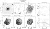
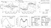
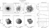
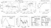
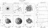
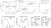
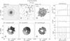
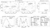
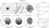
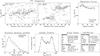
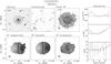
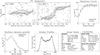
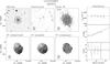
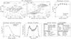
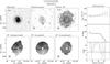
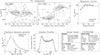
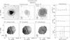
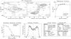
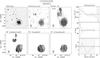
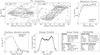
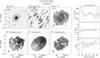
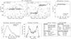
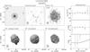
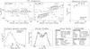
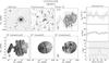
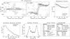
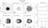
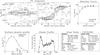
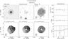
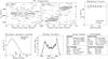
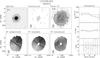
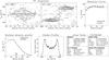
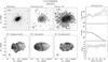
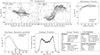
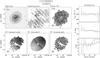
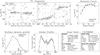
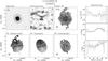
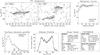
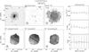
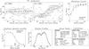
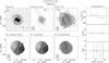
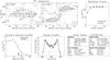
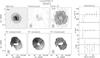
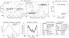
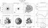
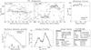
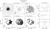
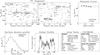
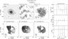
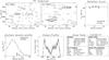
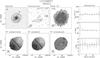
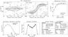
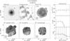
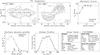
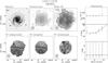
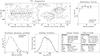
All Tables
All Figures
|
Fig. 1 Illustration of the trade-off between angular resolution and column-density sensitivity for different robust weightings of the WSRT visibility data, ranging from uniform to natural weighting. The solid curve indicates the size of the synthesized beam, and the dashed curve shows the 3σ column-density sensitivity in a single channel. |
| In the text | |
|
Fig. 2 Comparison of our measurements with data from the literature. Left: total 21 cm radio continuum flux densities. Middle: integrated Hi line fluxes. Right: Hi line widths at the 20% level of peak intensity. Solid symbols represent data from the WSRT, open circles from the VLA, and open triangles from the GMRT. The data are listed in Table 3 with references to the literature values. |
| In the text | |
|
Fig. 3 Difference between the weighted-average, projected rotational velocities of the Hα, [Oiii] and Hi PV diagrams and half the corrected widths of the Hi global profiles. The dashed line shows the average difference while the rms scatter is indicated by the two dotted lines. |
| In the text | |
|
Fig. 4 Comparison of results from Hi observations with those from optical PPak observations. The figure shows differences between the systemic velocities (upper panel) and between position angles of the kinematic major axis in the inner regions of the galaxies (lower panel), measured from the Hi velocity fields and those measured with the PPak IFU from [Oiii] and stellar velocity fields (Paper VI). The dashed horizontal lines show the average differences. Solid points correspond to WSRT data, open circles to VLA data, and open triangles to GMRT data. |
| In the text | |
|
Fig. 5 Total and relative Hi masses as a function of MK (left), morphological type (middle), and B−K color (right). The dashed lines are fits to the DMS galaxies (black symbols). The gray symbols shows the galaxies from Verheijen & Sancisi (2001). |
| In the text | |
|
Fig. 6 Upper panel: correlation between the total Hi mass (ℳHI) and the beam-corrected diameter of the Hi disk (DHI = 2RHI). The solid line shows the fit to the data while the dashed line represents the correlation found by Verheijen & Sancisi (2001). Lower panel: average Hi mass surface density within RHI versus DHI. The line indicates the expected slope based on the fit in the upper panel. |
| In the text | |
|
Fig. 7 Comparison of the relative kinematic scale lengths of the stellar disks and the relative size of the Hi disks. Galaxies in which the stellar velocity dispersion decreases faster with radius than expected on the basis of the photometric scale length of the stellar disk (hσ/ 2hR< 1), tend to have relatively small Hi disks, and vice versa. |
| In the text | |
|
Fig. 8 Compilation of all 28 Hi column density profiles, divided in four non-equal bins for each of four global optical properties; morphological type, central disk surface brightness, absolute magnitude, and color. The profiles are scaled in radius by RHI. The horizontal dashed lines are drawn at the sample median |
| In the text | |
|
Fig. 9 Relations between the maximum, azimuthally-averaged Hi column densities ( |
| In the text | |
|
Fig. 10 Self-similarity of the Hi column density profiles. Upper panel: all 28 ΣHI profiles scaled in radius and normalized in amplitude. The thinnest lines correspond to the early-type spirals in our sample. The thick black line shows the clipped average profile and the dashed lines indicate the rms scatter at each radius. Lower panel: the crosses follow the thick black line in the upper panel and the dashed lines are identical to the dashed lines in the upper panel. Gray scales indicate steps of 0.5 times the rms scatter. The solid black line is the best-fit Gaussian function following the crosses above (ΣHI/ |
| In the text | |
|
Fig. 11 Compilation of all 28 derived rotation curves with different scalings for each panel. The sample of rotation curves is divided in two according to central disk surface brightness: gray curves correspond to galaxies of lower surface brightness ( |
| In the text | |
|
Fig. 12 Onset radii of the warps detected in the Hi disks, scaled by RHI (left) and R25 (right). Filled symbols indicate the onset radii of φ warps and open symbols indicate the onset radii of i warps. The solid black and gray lines show the straight average of the i warps and φ warps, respectively. The dashed gray line indicates R = 35″, the edge of the FOV of the PPak IFU. |
| In the text | |
|
Fig. 13 Distribution of 21 cm radio continuum luminosities. The solid histogram displays the distribution of 21 cm radio continuum luminosities of the galaxies in the reduced Hi sample. The dashed histogram shows the distribution for the IRAS galaxies as derived by Yun et al. (2001). |
| In the text | |
|
Fig. 14 Radio-infrared correlation of 15 galaxies in the reduced Hi sample detected by IRAS at 60 μm. Left: correlation between flux densities. The solid line indicates the simple relation S21cm = 0.01S60 μm. The dashed line shows the correlation found by Yun et al. (2001) for the IRAS 2 Jy sample. The vertical line indicates their lower flux-density limit of 2 Jy. Right: correlation between intrinsic radio and infrared luminosities. |
| In the text | |
|
Fig. 15 Relations between disk surface brightness ( |
| In the text | |
|
Fig. 16 Star formation density versus average Hi mass surface density for the galaxies in our sample (black) and the galaxies in Kennicutt (1998; gray). |
| In the text | |
Current usage metrics show cumulative count of Article Views (full-text article views including HTML views, PDF and ePub downloads, according to the available data) and Abstracts Views on Vision4Press platform.
Data correspond to usage on the plateform after 2015. The current usage metrics is available 48-96 hours after online publication and is updated daily on week days.
Initial download of the metrics may take a while.