| Issue |
A&A
Volume 585, January 2016
|
|
|---|---|---|
| Article Number | A120 | |
| Number of page(s) | 21 | |
| Section | Stellar structure and evolution | |
| DOI | https://doi.org/10.1051/0004-6361/201526074 | |
| Published online | 06 January 2016 | |
Massive star evolution in close binaries
Conditions for homogeneous chemical evolution
1
College of Science, Guizhou University, Guiyang, 550025
Guizhou Province
PR China
2
Geneva Observatory, Geneva University,
1290
Sauverny,
Switzerland
e-mail: This email address is being protected from spambots. You need JavaScript enabled to view it.
3
Key Laboratory for the Structure and Evolution of Celestial
Objects, Chinese Academy of Sciences, 650011
Kunming, PR
China
Received: 11 March 2015
Accepted: 20 August 2015
Abstract
Aims. We investigate the impact of tidal interactions, before any mass transfer, on various properties of the stellar models. We study the conditions for obtaining homogeneous evolution triggered by tidal interactions, and for avoiding any Roche lobe overflow (RLOF) during the main-sequence phase. By homogeneous evolution, we mean stars evolving with a nearly uniform chemical composition from the centre to the surface.
Methods. We consider the case of rotating stars computed with a strong core-envelope coupling mediated by an interior magnetic field. Models with initial masses between 15 and 60 M⊙, for metallicities between 0.002 and 0.014 and with initial rotation equal to 30% and 66% the critical rotation on the zero age main sequence, are computed for single stars and for stars in close binary systems. We consider close binary systems with initial orbital periods equal to 1.4, 1.6, and 1.8 days and a mass ratio equal to 3/2.
Results. In models without any tidal interaction (single stars and wide binaries), homogeneous evolution in solid body rotating models is obtained when two conditions are realised: the initial rotation must be high enough, and the loss of angular momentum by stellar winds should be modest. This last point favours metal-poor fast rotating stars. In models with tidal interactions, homogeneous evolution is obtained when rotation imposed by synchronisation is high enough (typically a time-averaged surface velocities during the main-sequence phase above 250 km s-1), whatever the mass losses. We present plots that indicate for which masses of the primary and for which initial periods the conditions for the homogenous evolution and avoidance of the RLOF are met, for various initial metallicities and rotations. In close binaries, mixing is stronger at higher than at lower metallicities. Homogeneous evolution is thus favoured at higher metallicities. RLOF avoidance is favoured at lower metallicities because stars with less metals remain more compact. We also study the impact of different processes for the angular momentum transport on the surface abundances and velocities in single and close binaries. In models where strong internal coupling is assumed, strong surface enrichments are always associated with high surface velocities in binary or single star models. In contrast, models computed with mild coupling may produce strong surface enrichments associated with low surface velocities. This observable difference can be used to probe different models for the transport of the angular momentum in stars. Homogeneous evolution is more easily obtained in models (with or without tidal interactions) with solid body rotation.
Conclusions. Close binary models help us to understand homogeneous massive stars, fast rotating Wolf-Rayet stars, and progenitors of long soft gamma-ray bursts, even at high metallicities.
Key words: binaries: general / stars: rotation / binaries: close / stars: magnetic field / stars: abundances / stars: Wolf-Rayet
© ESO, 2016
1. Introduction
A significant fraction of massive stars may belong to close binary systems (see, e.g. Sana et al. 2012, 2013). Tidal interaction in close binary systems can change the evolution of the primary well before any mass transfer (de Mink et al. 2009a; Song et al. 2013). In particular, strong mixing can be induced, leading to a nearly homogeneous evolution. Homogeneous evolution of stars is a topic of interest for many reasons. First, models and observations suggest the existence of these kinds of stars (Maeder 1987; Martins et al. 2009, 2013). Second, when occurring in close binary systems, this kind of homogeneous evolution may imply that the Roche lobe overflow (RLOF) is avoided (de Mink et al. 2009a). Third, this type of evolution may be of interest as a possible scenario leading to long soft gamma-ray burst (Yoon et al. 2006). Fourth, these stars are powerful sources of ionising photons (Meynet et al. 2008; Levesque et al. 2012; Leitherer et al. 2014) and if frequent enough in the early Universe could have contributed to its reionisation. Finally, homogeneous evolution may be also of interest in the context of studies aiming at understanding the anticorrelations between the abundances of some light elements like oxygen and sodium observed at the surface of a large fraction of stars in globular clusters (see discussions of the observational evidences and proposed models in the reviews by Gratton et al. 2004, 2012).
Homogeneous evolution can be triggered by various mechanisms:
-
1.
very massive stars have large enough convective cores that their evolution can be considered as nearly homogeneous (Maeder 1980; Yusof et al. 2013);
-
2.
strong internal mixing in radiative zones produce homogeneous evolution (Maeder 1987).
In this work, we focus on models with strong mixing in the radiative zones. This strong mixing can be due to either fast rotation and/or tidally induced shear mixing (TISM, see more below). Fast rotation can be the result of initial conditions, the star rotating fast on the zero age main sequence (ZAMS), or due to some accelerating mechanism induced by tidal forces, mass accretion or merging of stars.
Tidally induced shear mixing does not require any high initial rotation, it only requires the build up of strong shear gradients in the star. This mechanism only occurs in close binary systems, either when the star is spinning up or spinning down (Song et al. 2013), and only in stars that have mild internal transport processes of angular momentum (i.e. transports by shear and meridional currents).
In case the transport of angular momentum is quite fast every time (like that triggered by a strong internal magnetic field, as in the work of de Mink et al. 2009a, and as in most of our models), the star rotates nearly as a solid body and therefore the transport by the shear becomes negligible. The tidal interaction in that case mainly serves as a process to give the star a fast enough rotation to drive a homogeneous evolution. In the present work, we focus on these types of models. As such, it is a follow up of the study by de Mink et al. (2009a), with the following differences:
-
i)
In de Mink et al. (2009a), the space of parameters studied are massive binaries with initial masses 20 + 15 M⊙ and 50 + 25 M⊙, with a composition representative of the Small Magellanic Cloud (mass fraction of heavy elements Z = 0.0021) and with initial orbital periods between 1.1 and 4 days. Here we study binaries with initial masses 60 + 40 M⊙, 50 + 33.3 M⊙, 40 + 26.7 M⊙, 30 + 20 M⊙, and 15 + 10M⊙ for initial metallicities Z = 0.002, 0.007, and 0.014, and initial orbital periods equal to 1.4, 1.6, and 1.8 days.
-
ii)
In de Mink et al. (2009a), the synchronisation phase was not explicitly computed. Based on an analytical estimate of the synchronisation timescale, these authors showed that this time is very short, less than 1% of the main-sequence lifetime for the parameters considered in their work. Therefore, they began their computation assuming that the system is synchronised, and that the stars have rotation rates such that their spin period is equal to the orbital period. Here we explicitly compute the synchronisation phase accounting for the various transport processes. We compute models with high initial surface equatorial velocities between 360 and 420 km s-1 on the ZAMS (see Tables A.1 and A.2), corresponding to the cases of spin down by the tidal forces and models with moderate initial surface equatorial velocities between 150 and 175 km s-1 on the ZAMS, which correspond to the cases of spin up by the tidal forces.
-
iii)
The physical ingredients of our models are different from those used in de Mink et al. (2009a) (see more in Sect. 2 below). Also, in Appendix B, we explore the consequences of tidal interactions when two different transport mechanisms for angular momentum are considered. One that produces a mild coupling between the core and the envelope mediated by only shear and meridional currents and the other, which is a strong coupling, mediated by an internal magnetic field. As we see in later sections, the consequences of the tidal interactions are very different.
In Sect. 2, we discuss the physical ingredients of the models. The results for 40 M⊙ models, both single and in close binary system, are presented in Sect. 3. The models for stars with masses between 30 and 60 M⊙, with and without tidal interaction are discussed in Sect. 4. Section 5 discusses the conditions for obtaining a homogeneous evolution and for avoiding RLOF in a close binary system. Section 6 synthesises the conclusions and describes further observational and theoretical work that would benefit this line of research. Appendix A presents tables indicating some properties of the stellar models computed in this work. Appendix B is devoted to a discussion of the effects of tidal interactions on systems composed of a 15 and 10 M⊙ for two different treatments of the transport of angular momentum.
2. Physical ingredients of the models
Other than the effects of rotation and the tidal forces, the present models use the same physical ingredients as in the works by Ekström et al. (2012), Georgy et al. (2013a,b). In particular, we use the Schwarzschild criterion with a moderate overshoot for computing the size of the convective core. The overshooting parameter is taken equal to 10% the pressure scale height estimated at the border of the convective core given by the Schwarzschild’s criterion. The models by de Mink et al. (2009a) use a much higher overshooting parameter of 35.5% the pressure scale height estimated at the border of the Ledoux’s boundary, based on calibrations by Brott et al. (2011).
The impact of the tides in close binary system is accounted for as in Song et al. (2013). A significant difference, however, with respect to
the work by Song et al. (2013) is that here we assume
a strong internal coupling mediated by an internal magnetic field. More precisely, we
performed the computation including the equations of the Tayler-Spruit dynamo (Spruit 2002) as given in Maeder & Meynet (2005). In this framework, for the mixing of the chemical
species, we use the following equation: ![Mathematical equation: \begin{eqnarray*} \rho \frac{\text{d}X_i}{\text{d}t} = \frac{1}{r^2} \frac{\partial}{\partial r} \left( \rho r^2 \left[ D + D_\text{eff} \right] \frac{\partial X_i}{\partial r} \right) + \left( \frac{\text{d}X_i}{\text{d}t}\right)_\text{nucl}, \end{eqnarray*}](/articles/aa/full_html/2016/01/aa26074-15/aa26074-15-eq19.png) with ρ the density, Xi, the mass fraction of
element i,
t, the time,
r, the
radius, D and
Deff, the diffusion coefficients (see
below). The last last term on the right-hand side expresses the changes of the mass fraction
of element i
resulting from nuclear reactions. In the above expression, D = Dshear +
Dmagn with
with ρ the density, Xi, the mass fraction of
element i,
t, the time,
r, the
radius, D and
Deff, the diffusion coefficients (see
below). The last last term on the right-hand side expresses the changes of the mass fraction
of element i
resulting from nuclear reactions. In the above expression, D = Dshear +
Dmagn with
![Mathematical equation: \begin{eqnarray*} D_\text{shear}=f_\text{energ} \frac{H_P}{g\delta}\frac{K}{\left[\frac{\varphi}{\delta}\nabla_\mu + \left( \nabla_\text{ad} - \nabla_\text{rad} \right)\right]} \left( \frac{9\pi}{32}\ \Omega\ \frac{\text{d} \ln \Omega}{\text{d} \ln r} \right)^2, \end{eqnarray*}](/articles/aa/full_html/2016/01/aa26074-15/aa26074-15-eq28.png) where
where  , and with fenerg = 1, and
 . The quantity HP is the pressure scale
height, g, the
gravity, δ =
−(∂lnT/∂lnρ)μ,P,
∇ad,
∇rad and
∇μ
are the adiabatic, radiative temperature gradients and mean molecular weight gradient,
respectively, Ω, the angular
velocity, T,
the temperature, P, the pressure, κ, the opacity,
a, the
radiation constant, and c, the velocity of light. We also find
. The quantity HP is the pressure scale
height, g, the
gravity, δ =
−(∂lnT/∂lnρ)μ,P,
∇ad,
∇rad and
∇μ
are the adiabatic, radiative temperature gradients and mean molecular weight gradient,
respectively, Ω, the angular
velocity, T,
the temperature, P, the pressure, κ, the opacity,
a, the
radiation constant, and c, the velocity of light. We also find
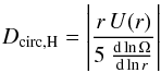
 with
with 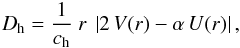 where
where  and ch = 1,
U(r) and V(r) are the
radial dependence of the vertical and horizontal component of the meridional circulation
velocity, respectively. To define the magnetic diffusivity Dmagn, we first
have to obtain the Alfven frequency ωA by solving the equation
and ch = 1,
U(r) and V(r) are the
radial dependence of the vertical and horizontal component of the meridional circulation
velocity, respectively. To define the magnetic diffusivity Dmagn, we first
have to obtain the Alfven frequency ωA by solving the equation
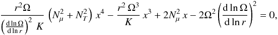 with
with  ,
,  and
and  . The parameter Dmagn comes then
as
. The parameter Dmagn comes then
as 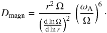 For the transport of the angular momentum, we
use the following equation:
For the transport of the angular momentum, we
use the following equation: 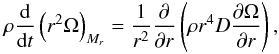 with D = Dshear +
Dmagn,Ω +
Dcirc,H. In this expression,
with D = Dshear +
Dmagn,Ω +
Dcirc,H. In this expression,
 and
and 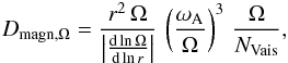 with the general Brunt-Väisälä frequency
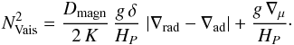 We consider that the minimum shear for the
dynamo to work is given by
We consider that the minimum shear for the
dynamo to work is given by  where
where 
As can be seen from the expression for the transport of the angular momentum, we accounted for the effect of meridional currents on the transport of the angular momentum through a diffusive instead of an advective equation as we usually do in models without magnetic fields. We can justify this approach with the following arguments: first, in models with magnetic fields, the distribution of angular momentum inside the star is dominated by the processes linked to the magnetic field, which involve diffusion and not by the meridional currents (which is an advective process); second, the transport by a magnetic field is so efficient that it imposes at every instant a nearly flat distribution of the angular velocity inside the star. Actually, the present models are equivalent to solid-body rotating models. If we had accounted for the meridional currents as an advective process, this would not have changed that conclusion and we checked that point numerically . Indeed, in Maeder & Meynet (2005), we checked that nearly solid-body rotation is achieved in models where the meridional currents are treated as an advective process and where the major processes governing the transport of the angular momentum are those associated with the magnetic instabilities. Keeping the advection by meridional currents for the transport of the angular momentum imposes the use of extremely short time steps and thus is very costly in CPU time. This would have made the computation of the ~100 different stellar models that we discuss impossible.
The dynamo theory proposed by Spruit (2002) has been criticised by Zahn et al. (2007). These last authors consider that the analytic treatment by Spruit (2002) is too simplified to be applied to the real stellar situation. On the other hand, the present models can be seen as a study of solid-body rotating models, whatever the physical cause is held responsible for building up this solid body rotation. Actually most of the chemical mixing is not due to the specific dynamo process, rather it is due to the meridional currents expected to be present in solid-body rotating stars. The concomitant effects of meridional currents and strong horizontal turbulence allow us to consider the mixing of the chemical species driven by these processes through a diffusive equation (diffusion coefficient Deff). Thus for the chemical mixing, in contrast to angular momentum, a diffusive treatment has to be applied.
Computations of the models, described in Sect. 1, were performed until the primary fills its Roche lobe. In case the primary does not succeed in filling in its Roche lobe, the computation was performed until the end of the main-sequence phase. For purpose of comparison, we performed computations of single star evolution for initial masses equal to the mass of the primaries and for the same initial rotational velocities as that considered in close binary systems.
As we see in the following, some of our models may enter a phase during which the mass fraction of hydrogen at the surface becomes lower than 0.3 and the effective temperature is larger than 4.0. In that case, we consider our model star to be a WRe, i.e. a Wolf-Rayet star (WR) defined from stellar evolution criteria. The WRe may not be exactly equivalent to the bona fide WR stars classified according to spectroscopic criteria (see, for instance, the discussion in Groh et al. 2014), however, there is some good overlap between these two definitions.
We calculated grids of single and binary stars in the range of masses 30 to 60 M⊙, with mass ratios equal to 3/2. We have considered three metallicities Z = 0.014, 0.007, and 0.002 to cover objects in the solar neighbourhood, the Large and Small Magellanic Clouds. A variety of orbital periods and of initial axial rotation velocities are considered, so that on the whole the evolutions of 96 different systems are calculated.
3. The 40 M⊙ stellar models
Before presenting a global overview of all the results, we first discuss the specific cases of 40 M⊙ models.
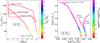 |
Fig. 1 Left panel: evolution of the surface equatorial velocity as a function of time for 40 M⊙ models. The colours indicate the ratio between the central and surface angular velocities. The orbital period for the binary model is 1.4 days, the secondary model has an initial mass equal to 26.7 M⊙. Right panel: evolutionary tracks in the HRD for the same models as in the left panel. The colours indicate the N/C ratio at the surface normalised to the initial one (N/Cini = 0.29 in mass fraction). In the binary systems, the stars initially have an angular velocity superior to the orbital velocity, and thus the tidal forces spin down the star (see Table A.1). |
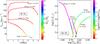 |
Fig. 2 Same as Fig. 1 for stars starting with a lower initial rotation (see Table A.2). In binary systems, the primary is spun-up by the tidal forces. |
In Figs. 1 and 2, the evolutions of the surface equatorial velocities (left panel) and of the tracks in the theoretical Hertzsprung-Russell (HR) diagram are shown (right panel) for both single and close binary 40 M⊙ stellar models (orbital period is 1.4 days). In Fig. 1, in binary systems, the primary star begins with an angular velocity larger than the orbital velocity and, thus, we have a spin-down case, while in Fig. 2, we have a spin-up case.
We first discuss the single star models. The most striking effect to be noted is that at the metallicity Z = 0.014, the surface velocity strongly decreases as a function of time as a result of the angular momentum losses driven by the stellar winds. This occurs for initially fast and moderately rotating models. The contrast with the angular velocity at the centre and the angular velocity at the surface is quite small, illustrating the strong coupling induced by the magnetic field. The core only begins to rotate significantly faster than the envelope at the very end of the main sequence. This comes from the ever increasing inhibiting effect of the μ-gradient at the border of the convective core during evolution. The μ-gradients decrease the transport via the magnetic field and, therefore, strong coupling. The contrast is stronger in models with Z = 0.014 than in the model with Z = 0.002. This comes from the fact that once the coupling between the core and the envelope is no longer achieved, higher mass loss rates at higher metallicities increase the contrast between the central and surface rotation rate more quickly.
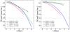 |
Fig. 3 Evolution of the surface hydrogen abundance (in mass fraction) for 40 M⊙ models. The limit for becoming a WR star (Xs< 0.3) is indicated with a gray dotted line. The models plotted are the same as those presented in Figs. 1 and 2. Left panel: cases of spin down. The Z = 0.014 and Z = 0.002 models have initial rotation on the ZAMS equal to 365 km s-1 and 391−394 km s-1, respectively (see Table. 1)). Right panel: cases of spin up. The Z = 0.014 and Z = 0.002 models have initial rotation on the ZAMS equal to 151 km s-1 and 163-167 km s-1, respectively. |
Looking at the tracks in the HR diagram, we see that the fast rotating model at high metallicity first begins to follow the typical blueward evolution, characterising a model evolving homogeneously. Then, because of the spin down by the stellar winds, the track bends toward the red. The starting point of the model with Z = 0.002 is shifted toward the blue because the star is more compact. This is mainly an opacity effect (see, e.g. the discussion in Mowlavi et al. 1998). Since that model loses much less angular momentum, the mixing driven by rotation remains quite high and the star follows a nearly homogeneous evolution.
In case of models starting with a lower initial rotation (see Fig. 2), we have qualitatively similar behaviours for the evolution of the surface velocity as those obtained for initially fast rotating stars, since the level of the surface rotation for single stars is simply shifted to lower values. This is the reason why for both metallicities considered in these plots, the evolutionary tracks for single stars evolve to the red part of the HRD as is normal for stars undergoing no or weak mixing in the radiative envelope.
We now consider close binary models. One of the main impacts of tidal interactions is changing the evolution of the surface rotation rates, as can be seen in Figs. 1 and 2. The changes of the surface rotation due to tidal forces is very rapid both in case of spin down (Fig. 1) and in case of spin up (Fig. 2).
Once synchronisation is achieved, the surface velocity keeps a more or less constant value for a significant part of the track (see Figs. 1 and 2). This is a consequence of the fact that the surface angular velocity is locked by the tidal interaction in a small domain around the orbital angular momentum velocity. Since the orbital angular velocity considered is the same for the case of spin up and spin down, the surface velocity obtained after synchronisation are very similar in both cases.
Models of 40 M⊙ with tidal interactions are more mixed than models without tidal interactions, both in case of spin down and in case of spin up for the orbital periods considered here. It is of course quite natural to expect that the spin-up model is more mixed than the single star. It is a little less obvious in the case of the spin-down model. At Z = 0.014, the spin-down model has a surface rotation velocity that is larger than the single star model. This results from the fact that the single star model loses much more angular momentum than the model in the close binary. The single star loses angular momentum by stellar winds. The star in the close binary also loses angular momentum by stellar winds, but the tidal interactions compensate for these losses to achieve synchronisation. This acceleration occurring in a close binary is accomplished through a transfer of angular momentum from the orbital reservoir to the star reservoir. Note that the amount of angular momentum in stars is very small with respect to the orbital angular momentum, so that this transfer hardly changes the orbital period and the distance between the components. Hence, for the conditions considered here, the spin-down model in a close binary system is more mixed than the single star mass-losing model.
At Z = 0.002, the surface velocity of the spin-down model is below the surface velocity of the single star most of the time, therefore, we should expect less mixing in the spin-down close binary model. However, this model follows a homogeneous evolution as the faster rotating model with no tidal interaction. What happens here is that both models (with and without tidal interaction) maintain sufficient angular momentum to be homogeneously mixed.
In Fig. 3, the evolution of the mass fraction of hydrogen at the surface of the 40 M⊙ stellar models are presented for the metallicities Z = 0.014 and 0.002. The single star models starting with a larger initial rotation rate (see black and green curves in the left panel) show stronger depletion of hydrogen at the surface than those starting with a lower initial rotation (see black and green curves in the right panel). In particular, the single star model at Z = 0.002, starting with an initial rotation of 391 km s-1, enters into the regime when the hydrogen mass fraction at the surface becomes lower than 0.3. The star becomes a WRe-type star (see Sect. 2).
The tracks of the close binary models are quite similar for the case of spin down and spin up, which is expected since these two models reach the same velocity at the surface very rapidly. The Z = 0.014 model stops at an earlier phase than the model at Z = 0.002 since it encounters the Roche limit, while the lower metallicity model avoids the Roche limit. This can be seen in Fig. 4, where the evolution as a function of time of the radii of the 40 M⊙ models are shown. The Z = 0.014 close binary model crosses the Roche limit at an age equal to 1.2 Myr (both in case of spin down and spin up), while due to strong mixing, the Z = 0.002 model never crosses the Roche limit during the whole MS phase.
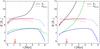 |
Fig. 4 Evolution of the stellar radius and Roche radius for the same models as in Fig. 3 (same colour code). The time at which the Roche radius is reached by the Z = 0.014 binary is marked with a red arrow. |
4. The whole grid of stellar models
To discuss the impact of the synchronisation process on our stellar models, we introduce below a few specific times:
-
tsync, the synchronisation timescale, defined here as the time for the surface angular velocity to approach the orbital angular velocity to less than 10%;
-
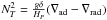
tN/C, the age of the star when, for the first time the ratio of nitrogen to carbon at the surface becomes larger than three times the initial ratio (N/Cini = 0.29 in mass fraction);
-
thom, the age of the star when the difference between the surface and central hydrogen mass fraction becomes larger than 10% of the central hydrogen mass fraction. Even in classical (non rotating) models with no extra mixing, since stars on the ZAMS are homogeneous, there is always a small period during which the mass fraction of hydrogen at the surface is equal or near to the mass fraction at the centre, and it takes some time for the central hydrogen to be depleted by more than 10%. Of course when mixing is active, this time is increased. To some extent, this time indicates the duration of the homogeneously evolving part of the stellar lifetime (indicated with blue shaded regions in Figs. 5 and 6). We say to some extent, because the evolutionary track in the HR diagram can present the characteristics of a homogeneous evolution even when the difference between the surface and central hydrogen mass fraction is larger than 10%, since homogeneous evolution also depends on the way hydrogen is distributed inside the model and not only on the difference between the mass fraction of hydrogen at the surface and at the centre.
-
tWR is the age of the star when it enters the WR phase (see Sect. 2).
-
t(end) is the age of the last computed model. This age corresponds approximately to the evolutionary stage when the primary fills its Roche volume (when this occurs) or the end of the main-sequence phase (when the filling of the Roche volume does not occur).
Figures 5 and 6 show how various times change as a function of the initial metallicity for different initial masses, rotations, and orbital periods (for binary systems)1. The synchronisation timescale is not shown since it is too short (shorter than tN/C). These figures allow us to see the impact of the tidal forces for various initial masses, rotations, and metallicities by comparing the upper panels corresponding to single star evolution and lower panels showing the situation when a companion is present. For each initial mass, the figures in the left column show cases of spin down, while the figures on the right column show cases of spin up.
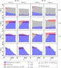 |
Fig. 5 tN/C (black triangles), thom (empty hexagons), tWR (crosses) and t(end), age of the last computed model (empty squares), as a function of metallicity. For each stellar model, with initial masses equal to 60 and 50 M⊙. These times are defined in the text in Sect. 3. The blue area corresponds to the part of the evolution that is homogeneous, the red region next to the WR phase. When the stellar models are neither homogeneous, nor a WR star, the region is shaded gray. When a R is indicated, it means that the model reaches a stage where RLOF occurs. |
4.1. Models of single stars
Before considering the effects of the tidal interactions, we discuss the results obtained for single star models or for stars in wide binary systems. In our previous works on rotating models, we showed that rotating models computed with no magnetic field present the following behaviour for what concerns the efficiency of rotational mixing: this efficiency increases with the initial mass, initial rotation and decreases with initial metallicity (see, e.g. discussions in Maeder & Meynet 2001; Ekström et al. 2012; Georgy et al. 2013a). From previous work, we know that models that have an internal magnetic field are more mixed (Maeder & Meynet 2005), but we have never investigated how mixing triggered by magnetic instabilities behaves when the initial mass, rotation, or metallicity vary. Actually, it happens that these dependencies are exactly the same (qualitatively) as those that were deduced from rotating non-magnetic models.
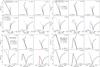 |
Fig. 7 Evolutionary tracks in the HR diagram for single star models and close binaries. The four panels correspond to different initial masses for the single star or for the primary in the close binary (in that case, the secondary has a mass equal to 2/3 the primary mass). The masses, the initial metallicities (Z), and the approximate initial surface velocities on the ZAMS are indicated. For the precise initial surface rotation of each model, see the values in Tables A.1 and A.2. For a given initial mass, the three upper panels correspond to spin-down cases, while the three lower panels correspond to spin-up cases. |
Mixing in magnetic models is more efficient in higher mass stars. For instance, we compare the positions of the triangles in the upper panels of Fig. 6 corresponding to the 40 and 30 M⊙ models with Ωini/ Ωcrit = 0.30 (the second and the fourth panel starting from left). We find that the stage at which the N/C ratio at the surface becomes superior to three times the initial ratio and corresponds to about half the main-sequence lifetime in the case of the 30 M⊙ at Z = 0.014, while it corresponds to about one-third of the MS lifetime for the corresponding model with an initial mass equal to 40 M⊙. This dependence on the initial mass is a result of the fact that U, the amplitude of the radial component of the meridional velocity, which is the main driving parameter for the chemical mixing in magnetic models, scales with the luminosity to mass ratio (see Eq. (11.75) in Maeder 2009) and this ratio increases with the initial mass.
As expected, mixing is more efficient in faster rotating models. Typically compare the positions of the triangles in Fig. 6 in the upper two right panels corresponding to single 30 M⊙ models. We see that when the initial rotation increases, triangles are shifted to smaller times indicating that in faster rotating models, mixing is more efficient. This comes from the fact that U scales with Ω.
At higher metallicities, the stellar models are less efficiently mixed. Again this can be observed by looking at the triangle positions in the upper right panel of Fig. 6. We see that for the spin-up 30 M⊙ stellar model, the time at which N/C at the surface becomes larger than three times the initial ratio is shifted toward larger ages when higher metallicities are considered. This comes mainly from the fact that, at high metallicities, stars are efficiently slowed down by the loss of angular momentum by stellar winds and thus are less mixed. In models with no strong stellar winds, two counteracting effects intervene that may, depending on the circumstances, trigger more or less mixing at high than at low metallicity. A rough estimate of the timescale for the mixing in the radiative zone can be obtained by the ratio of U to the radius of the star R (see Eq. (11.63) in Maeder 2009). On one hand, at higher metallicities, U is larger in the outer layers since U scales as the inverse of the density in this region, and stars, in metal-rich regions, are larger and hence less dense in their outer layers than stars in metal-poor regions. On the other hand, R is larger at high metallicity. Hence, the ratio U/R may increase or decrease with the metallicity. For the mass range we consider, the effect of the mass loss dominates and makes the mixing more efficient in low metallicity stars.
All the single star evolutionary tracks are shown in Fig. 7 (see black lines). For all the initial masses considered, the faster rotating tracks at Z = 0.002 have a homogeneous evolution. When the metallicity increases, the fast rotating tracks (see upper panels for each mass) begin to bend redwards at still earlier stages. The single star tracks computed for a moderate initial rotation (lower panels for each mass) all show a classical redward evolution during the MS phase. When the metallicity increases, the tracks are redder and less luminous.
4.2. Models of close binary stars
There are three main differences between the models with and without tidal interactions: changes in the surface velocity and composition, changes in the evolutionary tracks, and the possible occurrence of a RLOF event in close binary systems.
4.2.1. Synchronisation times
How does the synchronisation time vary with the initial mass, metallicity, rotation, and orbital period? For the models shown in Tables A.1 and A.2, tsync is always smaller than 0.8 Myr. In general, tsync is much shorter than this upper value and corresponds to a few percents of the MS lifetimes.
The synchronisation time increases with the difference between the initial Ω and the orbital period: see, for instance, the 30 M⊙ model at Z = 0.014; starting with an initial equatorial rotation velocity of 365 km s-1, the synchronisation time is 0.18 Myr when Ω /ωorb = 1.4, and equal to 0.43 Myr when Ω /ωorb = 1.8, (Ω is the stellar surface angular velocity and ωorb is the orbital angular velocity).
The dependency on the initial metallicity does appear quite weak. For instance the model B1.6, for a 30 M⊙ star that has an initial value of Ω /ωorb = 1.773 at Z = 0.007, has a value of tsync = 0.36 Myr. Model B1.4, for a 30 M⊙ star that has an initial value of Ω /ωorb = 1.772 at Z = 0.002, has a value of tsync = 0.34 Myr, i.e. not significantly different.
The synchronisation timescale decreases when larger initial masses are considered: compare, for instance, tsync for the 30 M⊙ model at Z = 0.007 with Ω /ωorb = 1.551, which is equal to 0.23 Myr, with the corresponding tsync value for the 60 M⊙ model at Z = 0.007 with Ω /ωorb = 1.557, which is equal to 0.08. The MS lifetime for the 60 M⊙ model is about 55% of the MS lifetime of the 30 M⊙ model, while tsync for the 60 M⊙ model is about one third the value of tsync for the 30 M⊙ model, indicating that tsync normalised to the MS lifetime decreases when higher initial mass stars are considered.
4.2.2. Surface and internal rotation rates
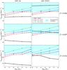 |
Fig. 8 Time-averaged surface equatorial velocity of single and binary stars as a function of the initial mass for various metallicities. The colour code for the lines is the same as in Fig. 7. The initial period in days is indicated. The results correspond to a companion having 2/3 the mass of the primary. The (cyan) big dots show the models that follow a homogeneous evolution. The cyan shading indicates the zone where homogeneous models lie in this diagram. The panels in the left column correspond to spin-down cases and the panels in the right column to spin-up cases. |
Time-averaged surface velocities for all the models as a function of the initial mass, metallicity, and orbital period are shown in Fig. 8. A few remarkable facts can be highlighted. 1) For single stars, the stronger mass loss for higher metallicities and higher stellar masses has a large impact on the velocity evolution, making the time-averaged surface velocities to decrease when the metallicity increases and when the initial mass increases. 2) In case of close binary stellar models, which are spinning down with tidal interactions (see the left panels), the spin down is well effective at low metallicity. The surface velocity in the close binary systems is always smaller than the surface velocity of the single star models. This is quite different at higher metallicities. For instance, at Z = 0.014, the surface velocity in the close binary systems is always larger than the surface velocity of the single star models. This might appear strange, since at the beginning we have a situation of spin down. What does happen here is that the spin down occurs only up to the point when synchronisation is achieved. Once synchronisation is reached, the transfer of angular momentum from the orbit to the star compensates for the losses of angular momentum by the star due to stellar winds. Thus, from that point on, an acceleration process sets in. 3) The time-averaged velocity in the close binary systems is slightly larger at higher than at lower metallicities. This comes from the fact that stars at high metallicities are larger than at low metallicities, implying that for a given surface angular velocity, imposed by synchronisation, the surface linear equatorial velocity is larger at high than at low metallicity2. 4) Globally the cases of spin up and spin down are very similar. The largest differences occur for the 60 M⊙ model at Z = 0.014 for a period equal to 1.4 days, the time-averaged surface velocity is equal to 400 km s-1 in the case of spin down and to 370 km s-1 in case of spin up. This comes from the fact that the synchronisation is obtained more rapidly in the spin-down case than in the spin-up case because the initial rotation in the spin-down case is much nearer from the synchronised one than in the case of spin down (see Table A.2).
All the models with tidal interactions show a very low degree of contrast between the central and the surface angular velocity.
4.2.3. Evolutionary tracks
All the tracks for the primaries in various close binary systems are shown in Fig. 7. For all the initial masses, the close binary tracks lay between the following two extreme cases: the single fastest rotating track at Z = 0.002 and the single slowest rotating track at Z = 0.014. We also see that the close binary tracks show great similarities between the spin-down case (upper panels for each mass) and spin-up case (lower panels for each mass), which is indeed expected. This is particularly visible with the 30 M⊙ model.
In the left panel of Fig. 9, we indicate the models that follow a homogeneous evolution. We used a very strict and conservative criteria for considering that a star follows a homogeneous evolution, namely, only the models evolving blueward along a straight line (until they enter into a WR phase) are considered to evolve homogeneously. There is no difference between the spin-down and spin-up cases. For each metallicity and initial mass, there exists an upper value for the orbital period below which stars evolve homogeneously. These upper limits are indicated in Table 1. The conditions for having a homogeneous evolution in close binary systems are more restricted at low than at high metallicities (the upper limits for the periods are smaller at Z = 0.002 than at Z = 0.014). We explain the reason for this in the next subsection.
All computations have been performed for a single value of the mass ratio between the secondary and primary equal to 2/3. One can wonder how things change when this ratio varies. For a given mass of the primary and a given initial orbital period, a higher mass ratio implies stronger tides and, thus, a more rapid synchronisation time. Note that keeping the period constant, assuming a more massive secondary star implies that the distance between the two components is larger, thus, a priori, it is not obvious that tides are stronger. This can however be seen using the third Kepler’s law and Eq. (6) in Paper I for the synchronisation time. Thus a higher mass ratio favours homogeneous evolution through the decrease of the synchronisation time3.
Maximum initial periods, Pmax, in days for having a homogeneous evolution for different initial mass stars (in solar masses) and metallicities and for a mass ratio of 3/2.
4.2.4. Mixing and Roche lobe overflow during the MS phase
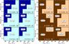 |
Fig. 9 Vertical axis is the initial orbital period in days; horizontal axis is the initial mass of the primary in a close binary system. The secondary has a mass equal to 2/3 the mass of the primary. The different panels correspond to different initial metallicities Z and to different initial rotation of the primary. The letters SD are for spin-down cases. The letters SU are for spin-up cases. Left panel: a homogeneous evolution during the main-sequence phase occurs where homog is indicated (light blue areas). Non-homogeneous evolution during the main-sequence phase occurs where non homog is indicated (dark blue areas). Right panel: Roche lobe overflow during the main-sequence phase is avoided where no RLOF is indicated (light brown areas). Roche lobe overflow during the main-sequence phase occurs where RLOF is indicated (dark brown areas). |
We begin by discussing the cases of the 30 M⊙ models in Fig. 6. Looking at the single models (see right upper panels of Fig. 6), we recall the following main features: mixing is higher when the initial rotation is higher and the metallicity lower. Also, at low metallicity the fast rotating model enters the WR phase at the end of the MS phase.
Now, when a companion is present with an orbital period between 1.4 and 1.8 days, in both the spin-down and spin-up models, stars are more mixed (see, for instance, how the triangles are shifted to smaller values in the binary models). The initially fast rotating model, which is spun down (lower panel in the third column), enters the WR stage at the very end of the MS phase at Z = 0.014, while the corresponding single model does not. As explained above, this is because although this model is spun down in a first phase, it is actually spun up after synchronisation to keep the surface angular velocity equal to the orbital angular velocity. This maintains a more rapid rotation than in the single star model, which is continuously spun down by stellar winds. For all of these models, RLOF occurs before the end of the MS phase. Therefore for these models, we have never a situation where the RLOF can be avoided during the MS phase.
In the case of the 60 M⊙ models, the same qualitative features as for the 30 M⊙ models can be seen for the plots representing the single star models. These more massive models are more mixed than the corresponding 30 M⊙ models. Binary models contain the following striking features: 1) As in the case of the 30 M⊙ model, stars with tidal interactions are more mixed, whether they belong to a system where a spin down or a spin up occurs. 2) Mixing does appear to be more efficient in binary system at higher than at lower metallicity, in strong contrast with what happens for single stars (see panels for the 60 M⊙ models for an orbital period equal to 1.8 days, which is less visible for the shorter periods because the models meet the Roche limit). We explain this behaviour change as follows: in the present models, the driving effects for chemical mixing are the meridional currents. It is well known that the meridional velocity in the outer layers varies as the inverse of the density. Models that are at higher metallicity have larger radii and thus shallower outer envelopes, and hence larger meridional currents. This situation favours mixing at higher metallicity. For single stars, however, mass loss by stellar winds may strongly reduce the angular momentum content and since meridional currents also scale with Ω, mass loss may counteract the above effect, resulting in weaker mixing at higher metallicity. In close binary systems, the tidal locking may maintain an angular momentum in the star that is larger than if the star evolved without any tidal interaction. In that case, Ω is kept constant and everything being equal (same mass), the model with a higher metallicity is more strongly mixed. This kind of effect is more marked in high-mass star models, which have a shallower envelope than in low initial mass stars. 3) In comparing the spin-up and the spin-down cases, we see that they are very similar given an orbital period. This is expected since the synchronisation timescale is short in both cases (although see the remark below) and the velocities to which the models converge are similar since imposed by the orbital period. A careful comparison between these two cases show, however, a slight asymmetry between the spin-down and spin-up cases: the spin-up cases are in general more mixed than the spin-down cases. This difference arises mostly because spin-up models start with initial angular velocities that are slightly closer to the orbital period than the spin-down models (see Tables A.1 and A.2). Moreover, as explained in Appendix B, in case of solid body rotation, the synchronisation time is shorter in case of spin up than in case of spin down. 4) All the 60 M⊙ models at Z = 0.002 avoid a RLOF during the MS phase (for the orbital periods considered here).
If we consider the panels for the two intermediate masses, 40 and 50 M⊙, we obtain qualitatively similar behaviours. Given an orbital period, the higher the initial mass, the stronger the effects of the tidal forces are (in all the cases the companion has a mass equal to 2/3 the mass of the primary).
In the right panel of Fig. 9, we indicate the models that do no go through a RLOF episode during the MS phase. Several findings are worth mentioning: 1) Every time a RLOF is avoided during the MS phase, the star has a homogeneous evolution, the only exception being the spin-down case for the 50 M⊙ at Z = 0.002. On the other hand, not all models having a homogeneous evolution avoid a RLOF episode during the MS phase. Therefore, the region of RLOF avoidance during the MS phase is in general smaller than the region of homogeneous evolution. This comes from the two opposite conditions for homogeneous evolution and RLOF avoidance: RLOF avoidance is more difficult when the initial periods are short, while homogeneous evolution is favoured by short periods. 2) RLOF avoidance is favoured for higher masses (more mixed) and lower metallicity (more compact) models. 3) Because of differences in the initial conditions for the spin-up and spin-down cases as well as differences in the synchronisation timescales, we have different situations in case of spin down and spin up. For this feature, initial conditions have a significant impact. In general the spin-up cases more often avoid a RLOF episode during the MS phase.
We discussed above the impact on the efficiency of the mixing of changing the mass ratio, keeping the mass of the primary and the initial orbital period the same. We indicated that a higher mass ratio favours shorter synchronisation time and thus stronger mixing. This effect favours RLOF avoidance, however, one has also to account for the variation of the Roche limit with the mass ratio. For a given mass of the primary and a given initial orbital period, the Roche limit is larger in systems with larger mass ratios4. This implies that a higher mass ratio favours RLOF avoidance.
5. Consequences of tidal interactions
As explained in the previous section, tidal interactions in sufficiently close systems trigger strong mixing. In the present models, this strong mixing is induced by the high rotation imposed by the tidal coupling.
We may wonder whether these binary models have an evolution equivalent to a single star starting its evolution on the ZAMS with a rotation equal to that obtained after synchronisation in the close binary system? The answer is no, especially at high metallicity. The main difference between these two cases is that the single star loses a lot of angular momentum via stellar winds while the component in the close binary system loses mass via stellar winds but not angular momentum, since the angular momentum lost by the winds is replenished at the expense of the orbital angular momentum via tidal interactions. Therefore in these systems, the close binary interaction is important to provide the star with a given initial rotation and for maintaining this rotation all along the evolution until RLOF episode occurs.
The strong mixing may induce a homogeneous evolution and thus, as was already found by de Mink et al. (2009a), may make the primary avoid a RLOF episode. From the present results, we can deduce the following conditions favouring this kind of scenario: first, obviously the orbital period should not be too small. For a given binary system, indeed, smaller the orbital period, the more difficult it will be to avoid RLOF even when stars are strongly mixed. Second, conditions are more favourable in more massive systems, which are those in which mixing is the strongest. For instance, none of the binary systems containing a 30 M⊙ model avoid RLOF during the MS phase, whatever the metallicity considered, while many cases of the systems with a 60 M⊙ models avoid this kind of an overflow during the MS phase. Finally, we see that a lower metallicity also constitutes a favourable condition for avoiding RLOF. Typically, all the considered binary systems with a 60 M⊙ model avoid RLOF during the MS phase at Z = 0.002, while at Z = 0.014 only the case with an orbital period equal to 1.8 days avoids it. Note that this last point may be surprising in view of our conclusion that models in close binary are more mixed at higher metallicities. We could have expected that if they are more mixed, they stay more compact, and thus would more easily avoid the RLOF. However, things are not so simple. Actually, stars are more mixed at higher metallicities because they have a more extended envelope and a more extended envelope makes it easier to reach the Roche limit. At low metallicities, stars remain more compact and this favours the avoidance of the RLOF.
We saw in the present work, that tidal interactions can provide sufficient angular momentum for triggering a homogeneous evolution to the primary close binary systems. This implies that the radiative envelope is rich in CNO-processed material at early times along the MS phase. Some mass is lost by the stellar winds and some mass can be lost at the moment of the mass transfer on the secondary in case the mass transfer is nonconservative. This material, lost by the system, if used to form new stars, produces stars with some signature of CNO processing. This might be a possible channel to explain second generation stars in globular clusters.
Close binaries have already been invoked in this context by de Mink et al. (2009b). These authors propose that the secondary is accelerated to the critical velocity through mass accretion from the primary. When the critical limit is reached, the mass lost by the primary can no longer be accreted by the secondary and, therefore, is lost in the interstellar medium. At that point, the primary may have lost sufficient mass for layers that have been processed at least partially by the CNO burning to be uncovered. This mass constitutes material that can be used to form new stars that would show surface abundances with signatures of CNO processing. In that scenario, therefore, the CNO processed matter is extracted from the primary because previous mass losses have uncovered H-burning regions and the mass is lost because the secondary has reached the critical velocity. In the scenario presented here, CNO processed material is obtained very early in the evolution because of the mixing triggered by tidal interactions. The mass at the moment of the mass transfer can be lost because of the same reason invoked by de Mink (the reaching of the critical limit by the secondary) or other effects. Typically, the secondary, if massive enough, loses some mass by stellar winds. This may prevent the secondary from accreting part or all the material lost from the primary. We shall discuss the impact of these models in the frame of the origin of the anticorrelations in globular clusters in a forthcoming paper.
Could this kind of an evolution be a plausible scenario for long soft gamma-ray bursts? At the moment, we cannot provide an answer to that question since it requires the computation of more advanced stages of the evolution of the systems. However, it is interesting that tidal interactions can trigger homogeneous evolution of the primary, makes it enter the WR phase at an early stage in its evolution, while keeping a high angular momentum content. Of course the story is not finished and it may be that there will be still some mass transfer when the secondary were to evolve in redder parts of the HRD. In cases, however, where no further mass transfer occurs or, if it occurs, that most of the mass were lost by the system, then the present scenario could be an interesting one for making fast rotating black holes from objects with no hydrogen-rich envelope. Interestingly, this scenario might explain the existence of a long soft gamma-ray burst even at high metallicity. Single fast rotating models with strong internal coupling lose a lot of angular momentum via stellar winds at high metallicity making the conditions for obtaining simultaneously a fast rotating black hole from a progenitor having lost its H-rich envelope very difficult. Here, as we saw, tidal interactions can do two things that are favourable for obtaining these conditions: they produce mixing and they replenish the star in spin angular momentum, even when mass is lost.
How can the present models be tested by observations? They can be checked through the observations of the surface abundances of short period binary systems before any mass transfer has occurred. These systems will most likely be synchronised in view of the very short timescale for this process to occur. The determination of the orbital period will also determine the axial rotation of the two components. If some indications are obtained on the initial mass, metallicity of the system, then the observed surface abundances can be compared to the predictions of the present computations. Note that whatever the initial rotation of the primary, the surface abundances will be the same after synchronisation. Hence, the initial rotation of the components is not a critical parameter, which is indeed a nice feature since this parameter cannot be estimated in a model independent way. Thus these close binary models represent very interesting targets to check rotational mixing (see also de Mink et al. 2009a).
Another prediction of the present models is that the primary of all close binary systems with an orbital period equal or inferior to 1.4 days, with a primary more massive than 40 M⊙, a companion having a mass equal to 2/3 of the primary, for metallicities Z equal or larger than 0.002 will follow a homogeneous evolution. Stars that follow a homogeneous evolution are overluminous for their mass. All these models at Z = 0.002 avoid a RLOF event during the MS phase.
Close binary evolution may produce very fast rotating WR stars, as can be seen from Tables A.1 and A.2. Indeed, an equatorial velocity between 160 and 360 km s-1 can be obtained through the binary channel. The corresponding single star models entering a WR phase have a surface velocity at that stage typically between 20 and 80 km s-1. Gräfener et al. (2012) deduced rotational properties inferred from photometric variability for six WR stars (see their Table 3 and references therein). Three of them present a surface velocity between 110 and 230 km s-1. Such a high surface velocity would be in good agreement with a close binary evolution.
6. Conclusions and perspectives
In this work, we studied the evolution of single and binary stellar models with a strong internal coupling.
For single stars, we showed that the mixing efficiency is stronger for the higher initial mass, initial rotation, and the lower metallicity. This is exactly the same as in models with a moderate coupling, although the physics for mixing between these two kinds of models is very different. In mildly coupled models, mixing is triggered by the gradients of Ω, while in strongly coupled models, it is driven by Ω. We also obtain that stars with a strong internal coupling are more strongly mixed than models with a moderate coupling (all other ingredients being kept the same).
When a companion is present, we checked that, as is well known, the synchronisation time is very short. Therefore, the main effect of the companion is to lock the rotation around the orbital rotation. The evolution after the synchronisation process depends on the angular momentum at the synchronisation time. The higher this angular momentum content, the higher the degree of mixing is. There is little dependence of the results on the initial velocity of the star. The angular momentum after synchronisation is of course the highest in the systems with the shortest orbital periods.
Large differences between single and close binary models with initial masses above about 30 M⊙ with similar initial rotation occur at high metallicity. The main difference comes from the fact that the single star model is spun down by losses of angular momentum by the stellar winds, while the angular momentum lost by the star in the close binary system is replenished by tidal interactions. In that case, mass loss induces an acceleration of the star once synchronisation is achieved.
In contrast with single star models, the higher the metallicity, the more efficient the mixing is, in the close binary models.
We have obtained some indications for the limiting orbital period below which our models will follow a homogeneous evolution. The conditions for homogeneous evolution are more restricted at low metallicity for the reason just mentioned above (less efficient mixing in low metallicity environments).
Quite generally, when no RLOF occurs during the MS phase, the star has a homogeneous evolution. Not all models evolving homogeneously avoid a RLOF episode. RLOF avoidance is favoured in high-mass star models at low metallicity.
How can we check these models through observations? Ideally, one would like to observe close eclipsing binaries for which it is possible to obtain the masses of the components and from spectroscopy their position in the HR diagram as well as some indications of their surface abundances. These systems should be observed at a stage before any mass transfer. They would be likely synchronised since synchronisation time is too short to allow the observation of a system before it is synchronised.
From an analysis of these data, we could check the following points: first, we can see whether these stars present surface enrichments. We see that for short enough periods, surface enrichments are predicted for many models, with or without magnetic fields5. Second, we can check whether stars are overluminous for their initial mass, indicating that indeed they are strongly mixed. Third, we can deduce their surface velocity. This last point is very important to discriminate between two classes of models: actually, the present models with strong internal coupling only predict strong mixing for models with high surface velocities (this is because the triggering of the mixing is Ω and not the gradient of Ω). On the other hand, models with mild internal mixing mainly driven by shear can produce models that are strongly mixed and show a low surface velocity (Song et al. 2013). Note that these characteristics can also be obtained in single star evolution models when braking occurs by magnetic coupling between the surface of the star and stellar wind (Meynet et al. 2011).
Finally, the present evolutionary scenario might be interesting to consider in the frame of the origin of the anticorrelation in globular clusters and to explain the progenitors of some long soft gamma-ray bursts especially those that might appear in metal-rich regions. Close binary evolution seems to be needed to explain the existence of fast rotating WR stars.
Appendix A tables include various properties of all the models computed here, among them the precise values of the times defined just above.
The angular surface velocity is determined by synchronisation and thus only depends on the orbital period, and not on the initial metallicity.
The angular velocity of the stars at synchronisation is fixed by the orbital period and, thus, provided this quantity is kept fixed, the mass ratio has no impact on the post-synchronisation angular velocity.
This comes from the fact that to keep the same orbital period in systems with more massive components, the distance between the two components needs to be larger.
Note that stars following a homogeneous evolution show a carbon to hydrogen ratio at the surface that decreases in a first phase and then increases. This non-monotonic behaviour comes from the fact that in these nearly homogeneous models, both carbon and hydrogen vary significantly. Since the CN equilibrium is reached very rapidly, the first phase corresponds to the decrease of carbon while the abundance of hydrogen changes little, and thus the C/H ratio decreases. The second increasing part of the curve comes from the carbon remaining more or less constant (it has reached the CNO equilibrium value), while the abundance of hydrogen decreases. This makes this ratio increase with time.
This is the case regardless of the physical cause imposing this solid body rotation.
Acknowledgments
The authors thank the anonymous referee who helped to improve this paper through very constructive remarks. This work was sponsored by the National Natural Science Foundation of China (Grant No. 11463002) and the Key Laboratory for the Structure and Evolution of Celestial Objects, Chinese Academy of Sciences (Grant No. OP201405). This work was supported by the Swiss National Science Foundation (project number 200020-146401).
References
- Brott, I., de Mink, S. E., Cantiello, M., et al. 2011, A&A, 530, A115 [NASA ADS] [CrossRef] [EDP Sciences] [Google Scholar]
- de Mink, S. E., Cantiello, M., Langer, N., et al. 2009a, A&A, 497, 243 [NASA ADS] [CrossRef] [EDP Sciences] [Google Scholar]
- de Mink, S. E., Pols, O. R., Langer, N., & Izzard, R. G. 2009b, A&A, 507, L1 [NASA ADS] [CrossRef] [EDP Sciences] [Google Scholar]
- Ekström, S., Georgy, C., Eggenberger, P., et al. 2012, A&A, 537, A146 [NASA ADS] [CrossRef] [EDP Sciences] [Google Scholar]
- Georgy, C., Ekström, S., Eggenberger, P., et al. 2013a, A&A, 558, A103 [NASA ADS] [CrossRef] [EDP Sciences] [Google Scholar]
- Georgy, C., Ekström, S., Granada, A., et al. 2013b, A&A, 553, A24 [NASA ADS] [CrossRef] [EDP Sciences] [Google Scholar]
- Gräfener, G., Vink, J. S., Harries, T. J., & Langer, N. 2012, A&A, 547, A83 [NASA ADS] [CrossRef] [EDP Sciences] [Google Scholar]
- Gratton, R., Sneden, C., & Carretta, E. 2004, ARA&A, 42, 385 [NASA ADS] [CrossRef] [Google Scholar]
- Gratton, R. G., Carretta, E., & Bragaglia, A. 2012, A&ARv, 20, 50 [CrossRef] [Google Scholar]
- Groh, J. H., Meynet, G., Ekström, S., & Georgy, C. 2014, A&A, 564, A30 [NASA ADS] [CrossRef] [EDP Sciences] [Google Scholar]
- Hunter, I., Brott, I., Langer, N., et al. 2009, A&A, 496, 841 [NASA ADS] [CrossRef] [EDP Sciences] [Google Scholar]
- Leitherer, C., Ekström, S., Meynet, G., et al. 2014, ApJS, 212, 14 [NASA ADS] [CrossRef] [Google Scholar]
- Levesque, E. M., Leitherer, C., Ekstrom, S., Meynet, G., & Schaerer, D. 2012, ApJ, 751, 67 [NASA ADS] [CrossRef] [Google Scholar]
- Maeder, A. 1980, A&A, 92, 101 [NASA ADS] [Google Scholar]
- Maeder, A. 1987, A&A, 178, 159 [NASA ADS] [Google Scholar]
- Maeder, A. 2009, Physics, Formation and Evolution of Rotating Stars (Berlin, Heidelberg: Springer) [Google Scholar]
- Maeder, A., & Meynet, G. 2001, A&A, 373, 555 [NASA ADS] [CrossRef] [EDP Sciences] [Google Scholar]
- Maeder, A., & Meynet, G. 2005, A&A, 440, 1041 [NASA ADS] [CrossRef] [EDP Sciences] [Google Scholar]
- Martins, F., Hillier, D. J., Bouret, J. C., et al. 2009, A&A, 495, 257 [NASA ADS] [CrossRef] [EDP Sciences] [Google Scholar]
- Martins, F., Depagne, E., Russeil, D., & Mahy, L. 2013, A&A, 554, A23 [NASA ADS] [CrossRef] [EDP Sciences] [Google Scholar]
- Meynet, G., Ekström, S., Maeder, A., et al. 2008, in IAU Symp. 250, eds. F. Bresolin, P. A. Crowther, & J. Puls, 147 [Google Scholar]
- Meynet, G., Eggenberger, P., & Maeder, A. 2011, A&A, 525, L11 [NASA ADS] [CrossRef] [EDP Sciences] [Google Scholar]
- Mowlavi, N., Meynet, G., Maeder, A., Schaerer, D., & Charbonnel, C. 1998, A&A, 335, 573 [NASA ADS] [Google Scholar]
- Sana, H., de Mink, S. E., de Koter, A., et al. 2012, Science, 337, 444 [Google Scholar]
- Sana, H., de Koter, A., de Mink, S. E., et al. 2013, A&A, 550, A107 [NASA ADS] [CrossRef] [EDP Sciences] [Google Scholar]
- Song, H. F., Maeder, A., Meynet, G., et al. 2013, A&A, 556, A100 [NASA ADS] [CrossRef] [EDP Sciences] [Google Scholar]
- Spruit, H. C. 2002, A&A, 381, 923 [NASA ADS] [CrossRef] [EDP Sciences] [Google Scholar]
- Yoon, S.-C., Langer, N., & Norman, C. 2006, A&A, 460, 199 [NASA ADS] [CrossRef] [EDP Sciences] [Google Scholar]
- Yusof, N., Hirschi, R., Meynet, G., et al. 2013, MNRAS, 433, 1114 [NASA ADS] [CrossRef] [Google Scholar]
- Zahn, J.-P., Brun, A. S., & Mathis, S. 2007, A&A, 474, 145 [NASA ADS] [CrossRef] [EDP Sciences] [Google Scholar]
Appendix A: Some properties of the stellar models
Some properties of the single and binary models computed in this work are presented in Tables A.1 and A.2. The first four columns specify the model considered providing information about its status as a single or a component in a binary system with a given orbital period, the ratio of the initial surface angular velocity to the critical velocity on the ZAMS, the ratio of the initial surface angular velocity to the orbital one, as well as the initial equatorial rotation velocity. The five following columns indicate, respectively, the different times defined at the beginning of Sect. 4. The last three columns give some properties of the last computed model: Xc(end) is the mass fraction of hydrogen at the centre, υeq(end) is the surface equatorial velocity, and N/C(end) the ratio at the surface of the mass fractions of nitrogen to carbon normalised to the initial ratio. The initial ratio is the same for the three metallicities and is equal to 0.29 in mass fraction.
Some properties of the single and binary models for initial masses equal to 30 M⊙ and 40 M⊙.
Some properties of the single and binary models for initial masses equal to 50 M⊙ and 60 M⊙.
Appendix B: Tidal interaction in close binary systems: impact of two different transport mechanisms for the angular momentum
In Paper I (Song et al. 2013), we studied the effects of tidal interaction in close binary systems consisting of a 15 and a 10 M⊙ star. We considered that the mechanisms for the transport of the angular momentum inside the star were the meridional currents and the shear instabilities. Here, we computed the models accounting for the Tayler-Spruit dynamo, which is a much more efficient transport mechanism for the angular momentum and which imposes, at every time, a distribution of the angular velocity inside the star very close to a solid body rotation. To see how these different transport mechanisms affect various properties of the single and close binary stars, we compare the results obtained for 15 M⊙ models computed with these two methods, starting with exactly the same initial conditions.
Appendix B.1: Spin-down case
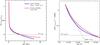 |
Fig. B.1 Left panel: evolution as a function of time of the surface angular velocity, Ω, minus the orbital angular velocity, ωorb, normalised to the orbital angular velocity for a 15 M⊙ model at Z = 0.014 beginning its evolution on the ZAMS with an initial rotation around 420 km s-1 and an orbital period equal to 1.4 days. Its companion has 10 M⊙. The solid (blue) line corresponds to models computed with a mild coupling mediated by shear and meridional currents. The dashed (red) line corresponds to models with a strong coupling mediated by an internal magnetic field (solid body rotation). The horizontal dotted line has an ordinate equal to 0, i.e. its intersection with the other curves indicates when an equality between Ω and ωorb is obtained. Right panel: evolution as a function of time of Ω − ωorb (natural logarithm) for the same models as in the left panel. The horizontal dotted line is at an ordinate equal to (Ω − ωorb) /e. The other dotted line has a slope equal to 1 /trot as given by Eq. (6) in Paper I. |
We discuss here the spin-down case for the 15 M⊙ model with a 10 M⊙ companion with an initial orbital period of 1.4 days. In Fig. B.1, we show the evolution of the difference between the actual surface angular velocity Ω and the orbital angular velocity ωorb for the cases without (solid line) and with an internal magnetic field (dashed line). The case without an internal magnetic field corresponds to a model already studied in Paper I (Song et al. 2013). The left panel of the figure shows the evolution of the difference between the actual surface angular velocity and the orbital velocity normalised to the orbital velocity. The right panel is a zoom on the very beginning of the slowing down process and shows the difference between the actual velocity and the orbital velocity with no normalisation.
We see that the evolution is quite similar in models with and without an internal magnetic field. This comes from the fact that at the beginning the two models present very similar characteristics (e.g. both are solid body rotating). Actually, we can see that both models very rapidly enter the regime where they have a surface angular velocity differing from the orbital velocity by less than 20%. This illustrates the well-known fact that indeed synchronisation is a very rapid process (see, e.g. the discussion in de Mink et al. 2009a).
How does the actual synchronisation timescale obtained by the numerical models compare to the values obtained from analytic formulae? An interesting quantity is trot (see, for instance, Eq. (6) in Paper I); trot corresponds to the time that is needed to decrease the quantity Ω − ωorb by a factor e (on the left panel of Fig. B.1, this corresponds to a decrease of one dex in the ordinate scale).
For evaluating trot from the analytical formula, we use the characteristics of the models on the ZAMS. The formula involves the moment of inertia of the region where the tidal force applies. Thus, this timescale varies a lot depending on which portion of the star is considered to estimate the moment of inertia. In case the moment of inertia of the whole star is considered, the time is obviously longer than when only the moment of inertia of the outer layer is considered. Formally plugging the moment of inertia of the whole star in the analytic formula implicitly assumes that any change of the angular momentum at the surface instantaneously has an impact on the angular momentum in the core. This corresponds to the strongest coupling we can imagine and implies the longest synchronisation time (the tides have to slow down the whole star and not only its outer layers. When transport by magnetic fields are assumed, we have a situation approaching that of an instantaneous redistribution). The case of considering the moment of inertia of only the outer layers would correspond to the other extreme case where there is no coupling between the core (or the region below these outer layers) and these outer layers. In that case, synchronisation is obtained more rapidly since a much smaller mass needs to be spun up or spun down. These examples show that numerical models with some moderate internal coupling lay in between these two cases.
Is it the situation obtained here by the numerical models? Yes it is. To see that, we consider the specific case of the 15 M⊙ model at Z = 0.014 in a close binary system with a companion of 10 M⊙ and with an orbital period of 1.4 days. The value for trot is equal to 38 100 years plugging the moment of inertia of the whole star in the analytic formula (Eq. (6) in Paper I). This timescale corresponds to about 0.3% of the main-sequence lifetime of a non-rotating solar metallicity 15 M⊙ model, whose main-sequence lifetime is about 11 My.
We now determine the time needed to decrease by a factor e the quantity Ω − ωorb from the numerical model. The value of ωorb corresponding to a period of 1.4 days is equal to 0.052 s-1. The horizontal dotted line on the right panel of Fig. B.1 shows the values (Ω − ωorb) /e. We see that the intersection between the curve showing Ω − ωorb (solid line) and the dotted line occurs at a time t = 0.174 Myr. Now the start time of the model is not 0, but the time t0 = 0.114 Myr because the model needs some time to settle into a ZAMS structure. Hence, the duration for decreasing Ω − ωorb by a factor e is equal to 174 000−114 000 = 60 000 years. Actually, this is above the value deduced from the analytic formula by about a factor 2.
This might be surprising at first sight when considering that the analytic formula should already be an upper limit, but the analytic formula is strictly valid only on a timescale during which Ω − ωorb does not vary too much. Actually, as can be seen from Fig. B.1, Ω − ωorb, decreases very rapidly (actually Ω varies very rapidly since ωorb keeps a constant value) and thus trot also varies very rapidly. Since Ω tends toward ωorb, trot increases, so that the actual time to decrease by a factor e can actually be larger than the value obtained from ZAMS properties. The increase is modest, however. Indeed, 60 000 years remains a very short value compared to the MS lifetime (less than 1%).
In the right panel of Fig. B.1, the slope at the beginning should be near the value given by 1 /trot. Interestingly, we can see that the slope at the ZAMS of the solid line (the model with shear and meridional currents without magnetic fields) is steeper than the slope of the dotted line, indicating that indeed at the beginning, the synchronisation time of the numerical model is shorter than that obtained by the analytic formula, as expected. We see also that the model with an internal magnetic field (dashed line) has an intermediate position between the solid and dotted line also exactly as expected. This short discussion therefore demonstrates that the present results are indeed quite consistent.
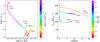 |
Fig. B.2 Left panel: evolutionary tracks in the HR diagram for 15 M⊙ at Z = 0.014, beginning their evolution on the ZAMS with initial rotation around 420 km s-1. The track labelled Single is for an isolate star computed as in Paper I (transport of angular momentum by shear and meridional currents), the track labelled with Binary is for a binary with an initial orbital period of 1.4 days computed with the same transport mechanisms as in Paper I. The models labelled Single+magn. and Binary+magn. are for single and binary stars, respectively, with similar characteristics, but computed with the Tayler-Spruit dynamo. The colour scales as the abundance ratio N/C at the surface normalised to the initial value on the ZAMS. Right panel: evolution of the surface equatorial velocity for the same models as in the left panel. The colour scales as the ratio Ωc/ Ωs. |
The time when Ω is equal to ωorb is around 3.5 Myr and 4 Myr for the non-magnetic and magnetic models, respectively (see the intersections of the horizontal dotted line with the curves on the left panel of Fig. B.1). However, from an observational point of view, the star can be synchronised much earlier when the difference between these two angular velocities is typically less than 10−20%. Indeed, uncertainties pertaining the measures of the rotation velocity and of the stellar radius (to obtain Ω from υrot) make it extremely difficult to identify the point when Ω is equal to ωorb. Moreover, as can be seen from Fig. B.1, the decrease of Ω is very rapid and important at the beginning making the star quasi-synchronised in a very short time interval. We note also that after the point when Ω = ωorb, Ω becomes slightly inferior to ωorb. This comes from the fact that the surface velocity of the star is governed by various processes with different timescales: the tidal forces that have a relatively long timescale when Ω is near ωorb, the inflation of the envelope (nuclear timescale), the mass loss (the process becomes more important when evolution proceeds and has a rapid timescale), the internal transport mechanisms (which are rapid in that case). The global effect of all these processes on the surface angular velocity results from their interplay. It is natural that when Ω is near ωorb, the tidal forces likely no longer dominate, at least until the differences between those two quantities are not too large, and thus Ω is maintained near ωorb but not exactly at a value equal to ωorb.
In Fig. B.2, the evolutionary tracks for the single 15 M⊙ model at Z = 0.014, with an initial rotation on the ZAMS equal to ~420 km s-1 is shown along with the tracks of models with the same characteristics, but now having a nearby 10 M⊙ companion (orbital period equal to 1.4 days). One case is the same as that presented in Paper I and the other is computed with the Tayler-Spruit dynamo.
When no magnetic field is accounted for, as in Paper I, we see that the model in the close binary system is more rapidly mixed than the single star model, hence, the small shift to the left with respect to the single star model. The additional mixing in the binary model is due to the tidally induced shear mixing as explained in Song et al. (2013).
When we account for the Tayler-Spruit dynamo, we see that the single star model is more mixed than the corresponding non-magnetic single star model. We even see that the mixing in that case is so efficient that the star follows the characteristic track of a nearly homogeneous star. This is in line with the results obtained by Maeder & Meynet (2005), who indeed noted that models with magnetic fields were more strongly mixed than models without magnetic fields, with all other ingredients kept the same. In this model, as is also true in the case of the binary model that we have discussed here, the mixing of the chemical elements is mainly governed by Deff, which itself depends on U and thus on Ω. This means that in these models, the value of Ω, and not that of the gradient of Ω (as in models of Song et al. 2013), governs the transport of the chemical elements.
The binary model computed with the Tayler-Spruit dynamo is spun down by the synchronisation process. Since Ω is lower than in the single star model, the stellar model is less mixed. Thus we see that a tidally induced spin down triggers more efficient mixing than for a single star in the case in which the angular momentum is transported by shear and meridional currents, and less efficient mixing than in a single star when the angular momentum transport imposes a solid body rotation6.
This is correct for the present 15 M⊙ model, which has weak stellar winds. When stellar winds are strong, a spin down can trigger more mixing provided that the angular momentum after synchronisation is high enough. Actually, as we have explained in Sect. 3, the spin down in these systems is rapidly replaced by a spin-up process triggered by the strong mass loss.
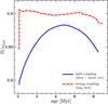 |
Fig. B.3 Evolution as a function of time of the ratio of the surface angular velocity to the orbital velocity for a 15 M⊙ model at Z = 0.014 with an initial rotation of 135 km s-1 and with an orbital period of 1.4 days. The solid lower curve corresponds to a model without magnetic fields and the dashed upper curve corresponds to a model with an internal magnetic field. |
An interesting consequence of this fact is that these models with strong coupling will never be able to explain the stars observed to be non-evolved, highly enriched, and slowly rotating stars (see group 2 stars discussed in Hunter et al. 2009). Models with milder coupling as those studied in Paper I or with a wind-magnetic braking mechanism (Meynet et al. 2011), in contrast, can produce stars showing these characteristics.
The binary model with a magnetic field is more mixed than the binary non-magnetic model. This is expected since the magnetic models are more mixed.
In the right panel of Fig. B.2, the evolution of the surface velocity is shown together with some indications on the internal gradient of angular velocity. The two single star models correspond to the upper lines. The surface velocity remains higher when the coupling is strong (magnetic coupling) than when the coupling is mild (coupling only due to shear and meridional currents). The single star model with an internal magnetic field has a very small contrast between the angular velocity at the centre and the angular velocity at the surface. In case of the close binary systems, the surface velocity rapidly converges in the two cases toward more or less the same value as a result of the tidal forces. The magnetic model, as in the single star case, shows a very weak contrast between the rotation of the core and that of the envelope.
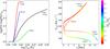 |
Fig. B.4 Left panel: evolution of the abundance ratio N/C at the surface of 15 M⊙ models at Z = 0.014 with an initial equatorial velocity of ~135 km s-1 as a function of lgTeff. Binary models correspond to 15 M⊙ with the same characteristics as indicated above but with a 10 M⊙ companion and an initial orbital period of 1.4 days. Right panel: evolution of the surface equatorial velocity as a function of time for the same models as in the left panel. The colours indicate the ratio between the central angular velocity and the surface velocity. |
Appendix B.2: Spin-up case
We now compare the cases with and without magnetic fields in case of spin up. In Fig. B.3, the evolution as a function of time of the ratio of the surface angular velocity to the orbital velocity is shown for the magnetic and the non-magnetic models. The magnetic model stabilises very rapidly around a value equal to 90% the orbital velocity. The non-magnetic model takes more time to reach the maximum value equal to 88% the orbital period before slowing down again.
Why does the surface angular velocity of the star never reach the orbital velocity? As noted above, the evolution of the surface angular velocity results from many effects: tidal forces tend to make Ω equal to ωorb, accelerating the star. On the other hand, the inflation of the radius, the transport of angular momentum inward due to meridional currents and the loss of angular momentum by stellar winds slow down the surface. The evolution shown in Fig. B.3 result from all these processes. The fact that the surface angular velocity of the star only approaches the orbital velocity indicates that the acceleration coming from the tidal interactions cannot compensate in these models for the counteracting effects of the other processes, thus, the synchronisation can only be achieved up to a certain point. However, observations could hardly detect this kind of situation very precisely: when the surface angular velocity is already equal to 85−90% of the orbital velocity, it will be difficult to assess that it is not equal to the orbital velocity in view of the uncertainties pertaining to the measures of the surface rotations of stars and of their radii (in order to obtain the surface angular velocity). The decrease of Ω toward the end of the computation results in part from larger mass loss rates and from more rapid inflation of the star.
In Fig. B.3, we can also see that the acceleration of the surface is more rapid in the magnetic than in the non-magnetic model. For the spin-down case, we just saw above that the synchronisation timescale increases when the coupling is stronger. Here we have the inverse situation. Why? In models with no magnetic field, we find that the meridional currents transport angular momentum from the surface to the core, thus, hiding an important amount of angular momentum deposited at
the surface in the central region. This tends to slow down the synchronisation process. In solid body rotating models, the core cannot rotate faster than the envelope, preventing the angular momentum from accumulating in the core. In that case, synchronisation is more rapid. Thus, we see that in case of spin down, a strong coupling makes the synchronisation time longer than in cases of milder coupling, while in case of spin up, a strong coupling makes the synchronisation time shorter.
The evolutionary tracks in the HRD for the 15 M⊙ stellar models at Z = 0.014 with an initial rotation rate around 135 km s-1 are very similar for single stars with or without an internal magnetic field. The same is true for the tracks of similar models in a close binary system with a 10 M⊙ companion with an initial orbital period of 1.4 days. This is why we do not show these tracks in a figure. The tracks do not differ much because these systems keep a relatively low velocity even in the case of spin up by tidal forces. These models follow classical evolution rather than homogeneous evolution.
On the other hand, the models at a given age present very different values at the surface for the N/C ratio and the equatorial velocity, as can be seen in Fig. B.4. Magnetic models are more mixed than non-magnetic models (whether single or in a binary system), binary models are more mixed than single models (whether magnetic or not), and the magnetic binary model is more mixed than the non-magnetic binary model. This last point is in contrast with the case of spin down, where the magnetic binary model was less mixed than the non-magnetic binary model. How can we explain this difference? As seen above, the spin-up timescale in the magnetic model is shorter than in the non-magnetic model, and thus the magnetic model reach levels of higher rotation earlier and have a higher mixing efficiency.
All Tables
Maximum initial periods, Pmax, in days for having a homogeneous evolution for different initial mass stars (in solar masses) and metallicities and for a mass ratio of 3/2.
Some properties of the single and binary models for initial masses equal to 30 M⊙ and 40 M⊙.
Some properties of the single and binary models for initial masses equal to 50 M⊙ and 60 M⊙.
All Figures
|
Fig. 1 Left panel: evolution of the surface equatorial velocity as a function of time for 40 M⊙ models. The colours indicate the ratio between the central and surface angular velocities. The orbital period for the binary model is 1.4 days, the secondary model has an initial mass equal to 26.7 M⊙. Right panel: evolutionary tracks in the HRD for the same models as in the left panel. The colours indicate the N/C ratio at the surface normalised to the initial one (N/Cini = 0.29 in mass fraction). In the binary systems, the stars initially have an angular velocity superior to the orbital velocity, and thus the tidal forces spin down the star (see Table A.1). |
| In the text | |
|
Fig. 2 Same as Fig. 1 for stars starting with a lower initial rotation (see Table A.2). In binary systems, the primary is spun-up by the tidal forces. |
| In the text | |
|
Fig. 3 Evolution of the surface hydrogen abundance (in mass fraction) for 40 M⊙ models. The limit for becoming a WR star (Xs< 0.3) is indicated with a gray dotted line. The models plotted are the same as those presented in Figs. 1 and 2. Left panel: cases of spin down. The Z = 0.014 and Z = 0.002 models have initial rotation on the ZAMS equal to 365 km s-1 and 391−394 km s-1, respectively (see Table. 1)). Right panel: cases of spin up. The Z = 0.014 and Z = 0.002 models have initial rotation on the ZAMS equal to 151 km s-1 and 163-167 km s-1, respectively. |
| In the text | |
|
Fig. 4 Evolution of the stellar radius and Roche radius for the same models as in Fig. 3 (same colour code). The time at which the Roche radius is reached by the Z = 0.014 binary is marked with a red arrow. |
| In the text | |
|
Fig. 5 tN/C (black triangles), thom (empty hexagons), tWR (crosses) and t(end), age of the last computed model (empty squares), as a function of metallicity. For each stellar model, with initial masses equal to 60 and 50 M⊙. These times are defined in the text in Sect. 3. The blue area corresponds to the part of the evolution that is homogeneous, the red region next to the WR phase. When the stellar models are neither homogeneous, nor a WR star, the region is shaded gray. When a R is indicated, it means that the model reaches a stage where RLOF occurs. |
| In the text | |
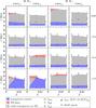 |
Fig. 6 Same as Fig. 5 for initial masses equal to 40 and 30 M⊙. |
| In the text | |
|
Fig. 7 Evolutionary tracks in the HR diagram for single star models and close binaries. The four panels correspond to different initial masses for the single star or for the primary in the close binary (in that case, the secondary has a mass equal to 2/3 the primary mass). The masses, the initial metallicities (Z), and the approximate initial surface velocities on the ZAMS are indicated. For the precise initial surface rotation of each model, see the values in Tables A.1 and A.2. For a given initial mass, the three upper panels correspond to spin-down cases, while the three lower panels correspond to spin-up cases. |
| In the text | |
|
Fig. 8 Time-averaged surface equatorial velocity of single and binary stars as a function of the initial mass for various metallicities. The colour code for the lines is the same as in Fig. 7. The initial period in days is indicated. The results correspond to a companion having 2/3 the mass of the primary. The (cyan) big dots show the models that follow a homogeneous evolution. The cyan shading indicates the zone where homogeneous models lie in this diagram. The panels in the left column correspond to spin-down cases and the panels in the right column to spin-up cases. |
| In the text | |
|
Fig. 9 Vertical axis is the initial orbital period in days; horizontal axis is the initial mass of the primary in a close binary system. The secondary has a mass equal to 2/3 the mass of the primary. The different panels correspond to different initial metallicities Z and to different initial rotation of the primary. The letters SD are for spin-down cases. The letters SU are for spin-up cases. Left panel: a homogeneous evolution during the main-sequence phase occurs where homog is indicated (light blue areas). Non-homogeneous evolution during the main-sequence phase occurs where non homog is indicated (dark blue areas). Right panel: Roche lobe overflow during the main-sequence phase is avoided where no RLOF is indicated (light brown areas). Roche lobe overflow during the main-sequence phase occurs where RLOF is indicated (dark brown areas). |
| In the text | |
|
Fig. B.1 Left panel: evolution as a function of time of the surface angular velocity, Ω, minus the orbital angular velocity, ωorb, normalised to the orbital angular velocity for a 15 M⊙ model at Z = 0.014 beginning its evolution on the ZAMS with an initial rotation around 420 km s-1 and an orbital period equal to 1.4 days. Its companion has 10 M⊙. The solid (blue) line corresponds to models computed with a mild coupling mediated by shear and meridional currents. The dashed (red) line corresponds to models with a strong coupling mediated by an internal magnetic field (solid body rotation). The horizontal dotted line has an ordinate equal to 0, i.e. its intersection with the other curves indicates when an equality between Ω and ωorb is obtained. Right panel: evolution as a function of time of Ω − ωorb (natural logarithm) for the same models as in the left panel. The horizontal dotted line is at an ordinate equal to (Ω − ωorb) /e. The other dotted line has a slope equal to 1 /trot as given by Eq. (6) in Paper I. |
| In the text | |
|
Fig. B.2 Left panel: evolutionary tracks in the HR diagram for 15 M⊙ at Z = 0.014, beginning their evolution on the ZAMS with initial rotation around 420 km s-1. The track labelled Single is for an isolate star computed as in Paper I (transport of angular momentum by shear and meridional currents), the track labelled with Binary is for a binary with an initial orbital period of 1.4 days computed with the same transport mechanisms as in Paper I. The models labelled Single+magn. and Binary+magn. are for single and binary stars, respectively, with similar characteristics, but computed with the Tayler-Spruit dynamo. The colour scales as the abundance ratio N/C at the surface normalised to the initial value on the ZAMS. Right panel: evolution of the surface equatorial velocity for the same models as in the left panel. The colour scales as the ratio Ωc/ Ωs. |
| In the text | |
|
Fig. B.3 Evolution as a function of time of the ratio of the surface angular velocity to the orbital velocity for a 15 M⊙ model at Z = 0.014 with an initial rotation of 135 km s-1 and with an orbital period of 1.4 days. The solid lower curve corresponds to a model without magnetic fields and the dashed upper curve corresponds to a model with an internal magnetic field. |
| In the text | |
|
Fig. B.4 Left panel: evolution of the abundance ratio N/C at the surface of 15 M⊙ models at Z = 0.014 with an initial equatorial velocity of ~135 km s-1 as a function of lgTeff. Binary models correspond to 15 M⊙ with the same characteristics as indicated above but with a 10 M⊙ companion and an initial orbital period of 1.4 days. Right panel: evolution of the surface equatorial velocity as a function of time for the same models as in the left panel. The colours indicate the ratio between the central angular velocity and the surface velocity. |
| In the text | |
Current usage metrics show cumulative count of Article Views (full-text article views including HTML views, PDF and ePub downloads, according to the available data) and Abstracts Views on Vision4Press platform.
Data correspond to usage on the plateform after 2015. The current usage metrics is available 48-96 hours after online publication and is updated daily on week days.
Initial download of the metrics may take a while.