| Issue |
A&A
Volume 584, December 2015
|
|
|---|---|---|
| Article Number | A15 | |
| Number of page(s) | 9 | |
| Section | Stellar atmospheres | |
| DOI | https://doi.org/10.1051/0004-6361/201526903 | |
| Published online | 13 November 2015 | |
Research Note
HARPS spectropolarimetry of three sharp-lined Herbig Ae stars: New insights ⋆,⋆⋆
1
Leibniz-Institut für Astrophysik Potsdam (AIP),
An der Sternwarte 16,
14482
Potsdam, Germany
e-mail: This email address is being protected from spambots. You need JavaScript enabled to view it.
2
European Southern Observatory, Karl-Schwarzschild-Str. 2, 85748
Garching,
Germany
3
Finnish Centre for Astronomy with ESO (FINCA), University of
Turku, Väisäläntie
20, 21500
Piikkiö,
Finland
4
Niels Bohr Institute & Centre for Star and Planet Formation,
University of Copenhagen, Øster
Voldgade 5, 1350
Copenhagen,
Denmark
5
Pulkovo Observatory, 196140
Saint-Petersburg,
Russia
6
Saint Petersburg State University, Universitetski pr. 28, 198504
Saint Petersburg,
Russia
7
Observatório Nacional/MCTI, Rua General José Cristino 77, CEP 20921-400
Rio de Janeiro, RJ, Brazil
Received: 6 July 2015
Accepted: 14 October 2015
Abstract
Aims. Recently, several arguments have been presented that favour a scenario in which the low detection rate of magnetic fields in Herbig Ae stars can be explained by the weakness of these fields and rather large measurement uncertainties. Spectropolarimetric studies involving sharp-lined Herbig Ae stars appear to be a promising approach for the detection of such weak magnetic fields. These studies offer a clear spectrum interpretation with respect to the effects of blending, local velocity fields, and chemical abundances, and allow us to identify a proper sample of spectral lines appropriate for magnetic field determination.
Methods. High-resolution spectropolarimetric observations of the three sharp-lined (vsini< 15 km s-1) Herbig Ae stars HD 101412, HD 104237, and HD 190073 have been obtained in recent years with the HARPS spectrograph in polarimetric mode. We used these archival observations to investigate the behaviour of their longitudinal magnetic fields. To carry out the magnetic field measurements, we used the multi-line singular value decomposition (SVD) method for Stokes profile reconstruction.
Results. We carried out a high-resolution spectropolarimetric analysis of the Herbig Ae star HD 101412 for the first time. We discovered that different line lists yield differences in both the shape of the Stokes V signatures and their field strengths. They could be interpreted in the context of the impact of the circumstellar matter and elemental abundance inhomogeneities on the measurements of the magnetic field. On the other hand, due to the small size of the Zeeman features on the first three epochs and the lack of near-IR observations, circumstellar and photospheric contributions cannot be estimated unambiguously. In the SVD Stokes V spectrum of the SB2 system HD 104237, we detect that the secondary component, which is a T Tauri star, possesses a rather strong magnetic field ⟨Bz⟩ = 129 ± 12 G, while no significant field is present in the primary component. Our measurements of HD 190073 confirm the presence of a variable magnetic field and indicate that the circumstellar environment may have a significant impact on the observed polarization features.
Key words: stars: pre-main sequence / stars: variables: general / stars: magnetic field / stars: individual: HD 101412 / stars: individual: HD 104237 / stars: individual: HD 190073
Based on data obtained from the ESO Science Archive Facility. Observations were made with ESO telescopes on La Silla Paranal Observatory under programme IDs 085.D-0296(A), 187.D-0917(A, D), and 089.D-0383(A).
Appendices are available in electronic form at http://www.aanda.org
© ESO, 2015
1. Introduction
Magnetic fields are of fundamental importance for intermediate-mass star formation and accretion-ejection processes (e.g. Li et al. 2009). However, as of today, no consistent scenario exists that explains how magnetic fields in Herbig Ae/Be stars are generated and how they interact with the circumstellar environment. Studies of the magnetic field topology using high-resolution spectropolarimetry are extremely important. They enable us to improve our understanding of magnetically driven accretion and outflows in these stars. Recently, Hubrig et al. (2015) presented several arguments favouring a scenario in which the low detection rate of magnetic fields in Herbig Ae stars can be explained by the weakness of these fields and rather low measurement accuracies. Notably, the authors show that using high-resolution High Accuracy Radial velocity Planet Searcher (HARPS) spectropolarimetric observations, even very weak magnetic fields, of the order of tens of gauss, can be detected in sharp-lined (vsini< 15 km s-1) Herbig Ae stars with an uncertainty of only a few gauss if the singular value decomposition (SVD) method is applied (Hubrig et al. 2015). In that work, a mean longitudinal magnetic field ⟨Bz⟩ = 33 ± 5 G was detected in the HARPS spectra of the sharp-lined Herbig Ae star PDS 2 with v sin i = 12 ± 2 km s-1. Similar accuracies have been reached, for example, for cool stars (e.g. Waite et al. 2015; Donati et al. 2011) with other high-resolution spectropolarimeters, like ESPaDOnS and Narval.
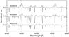 |
Fig. 1 Example spectra of the three sharp-lined Herbig Ae stars HD 101412, HD 104237, and HD 190073. |
A number of spectropolarimetric HARPS observations of three other sharp-lined Herbig Ae stars, HD 101412, HD 104237, and HD 190073 (see Fig. 1), are publicly available in the European Southern Observatory (ESO) archive. In contrast to low-resolution spectropolarimetry where hydrogen Balmer lines are the main contributors to the magnetic field measurements, high-resolution polarimetric spectra allow us to study in detail surface abundance inhomogeneities and, in particular, how different elements are distributed with respect to the magnetic field geometry. An inhomogeneous chemical abundance distribution is observed most frequently on the surface of upper-main-sequence Ap/Bp stars with large-scale organized magnetic fields. The abundance distribution of certain elements in these stars is usually non-uniform and non-symmetric with respect to the rotation axis, but shows a kind of relationship between the magnetic field geometry and the element spots. As an example, rare earth spots are usually found in the vicinity of magnetic poles, while iron peak elements are concentrated closer to the magnetic equator. It is possible that a similar kind of relationship exists in Herbig Ae stars. In addition to the three stars studied in this paper and PDS 2, the sample of Alecian et al. (2013b) adds only four more targets to the sharp-lined sample.
In Sect. 2, we describe the observations and data reduction of these three objects, and in Sect. 3 we present the method and results of our magnetic field measurements. Finally, in Sect. 4 we discuss the importance of the obtained results for our knowledge of the role of magnetic fields in intermediate-mass, pre-main-sequence stars.
2. Observations and data reduction
Seven observations of HD 101412, one data set for the Herbig Ae SB2 system HD 104237, and two data sets for the Herbig Ae star HD 190073 were obtained in recent years with the HARPS polarimeter (HARPSpol; Snik et al. 2008) attached to ESO’s 3.6 m telescope (La Silla, Chile). In Table 1, the heliocentric Julian dates of the observations are presented in the second column, followed by the rotation phase (if known) and the achieved peak signal-to-noise ratio (S/N) in the Stokes I spectra. Only for HD 101412 the rotation period of 42.076 d was determined in the past (Hubrig et al. 2011b). The archival data covers the rotation phases 0.131–0.297. The HARPSpol observations are usually split into several subexposures obtained with different orientations of the quarter-wave retarder plate relative to the beam splitter of the circular polarimeter. The spectra have a resolving power of about R = 115 000 and cover the spectral range 3780–6910 Å, with a small gap between 5259 and 5337 Å. The reduction and calibration of the archive spectra was performed using the HARPS data reduction software available at the ESO headquarters in Germany. The normalization of the spectra to the continuum level consisted of several steps described in detail by Hubrig et al. (2013). The Stokes I and V parameters were derived following the ratio method described by Donati et al. (1997). Null polarization spectra were calculated by combining the subexposures in such a way that polarization cancels out.
3. Magnetic field measurements
The multi-line SVD method was already successfully applied to high-resolution intensity spectra more than ten years ago by Barnes (2004), and the application to intermediate-resolution spectra was presented even earlier (Rucinski 1992; Rucinski et al. 1993). The software package used to study the magnetic fields in this paper, the SVD method for Stokes profile reconstruction, was introduced by Carroll et al. (2012). The basic idea of SVD is similar to the principal component analysis (PCA) approach, where the similarity of the individual Stokes V profiles allows one to describe the most coherent and systematic features present in all spectral line profiles as a projection onto a small number of eigenprofiles. The line masks for each star, based on their atmospheric parameters, are constructed using the VALD database (e.g. Kupka et al. 2000) following the basic principles stated already by Donati et al. (1997) for the least-squares deconvolution (LSD) technique. Here, we have used lines with intrinsic depths larger than 10%, while hydrogen Balmer lines, strong He i, and strong resonance lines are excluded. Also lines appearing close to telluric lines are removed from the mask. The SVD method is especially important for the extraction of polarized signals (Stokes V), which are frequently hidden below the noise level, while the reconstruction of the intensity profile (Stokes I) does not need the generally time-consuming application of the SVD technique.
Logbook of the HARPS spectropolarimetric observations.
The presence of δ Scuti-like pulsations is known (Böhm et al. 2004) for the Herbig Ae star HD 104237. These types of
pulsations were detected in a few Herbig Ae stars in the past (e.g. Kallinger et al. 2008). Nothing is known about pulsations in the Herbig
Ae stars HD 101412 and HD 190073. Since pulsations are known to have an impact on the
analysis of the presence of a magnetic field and its strength (e.g. Schnerr et al. 2006; Hubrig et al.
2011a), as a first step, we checked that no changes in the line profile shape or
radial velocity shifts are present in the obtained spectra on a short timescale of about ten
minutes for HD 101412 and on a timescale of ten to 30 min for HD 190073. These timescales
correspond to the exposure times of the individual subexposures during the observations of
these stars. For all three stars, the behaviour of the line profiles in the individual
subexposures is described in Appendix A. No indication
for variability on a short timescale was found for HD 101412 and HD 190073. In the following
subsections, we present the results of the magnetic field measurements for each star
separately. The longitudinal magnetic field ⟨Bz⟩ is measured by
calculating the first-order moment of the Stokes V profile (e.g. Mathys 1989) ![Mathematical equation: \begin{equation} \left<B_{z}\right> = -2.4 \times 10^{11}\frac{\int \upsilon V (\upsilon){\rm d}\upsilon }{\lambda_{0}g_{0}c\int [I_{\rm c}-I(\upsilon )]{\rm d}\upsilon}, \end{equation}](/articles/aa/full_html/2015/12/aa26903-15/aa26903-15-eq12.png) (1)where υ is the Doppler velocity in
km s-1, and
λ0
and g0 are the normalization values of the
wavelength and the average Landé factor.
(1)where υ is the Doppler velocity in
km s-1, and
λ0
and g0 are the normalization values of the
wavelength and the average Landé factor.
3.1. HD 101412
Previously published mean longitudinal magnetic field measurements of the Herbig Ae star HD 101412 have been carried out using low-resolution polarimetric spectra obtained with FORS 1/2 (FOcal Reducer low dispersion Spectrograph) mounted on the 8-m Antu telescope of the VLT (e.g. Wade et al. 2005, 2007; Hubrig et al. 2009, 2010, 2011b).
For each sample, the signal-to-noise ratio achieved in the SVD spectra and the measured longitudinal magnetic field are presented. The average Landé factor used in the SVD measurements is also indicated.
The fundamental parameters, Teff = 8300 K and log g = 3.8, and the projected rotation velocity, v sin i = 3 ± 2 km s-1, were determined by Cowley et al. (2010). The inspection of the SVD I, V, and N spectra in the phase range 0.131–0.297 obtained using a sample of 650 metallic lines reveals that the amplitude of the Zeeman features increases towards the later epochs and that the majority of these features have a shape typical of that observed in classical magnetic stars during crossover, i.e. in the phase interval when the magnetic field changes its polarity (e.g. Hubrig et al. 2014). For all observations, the null spectra appear flat, indicating the absence of spurious polarization. Using the false alarm probability (FAP; Donati et al. 1992), we obtain definite magnetic field detections with FAP < 10-10 on all epochs. The SVD I, V, and N for this line mask are presented in Fig. 2 (see also Fig. B.1, first column). Surprisingly, we detect in the SVD Stokes V profiles obtained for the first three epochs distinct features appearing as a second maximum in the red wings of the Zeeman profiles. Furthermore, these profiles seem to be slightly shifted to the blue by about 4 km s-1. This behaviour probably indicates that we observe contamination by the surrounding warm circumstellar (CS) matter in the form of wind. This scenario seems to be in agreement with the previous finding of Hubrig et al. (2009), who reported a strong contamination of UVES spectra of this star by weak lines of neutral and ionized iron (see their Fig. 6), where the lines of neutral iron are far more numerous than those of ionized iron.
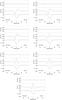 |
Fig. 2 The correspondence of SVD I, V, and N profiles of HD 101412 obtained using a sample of 650 lines belonging to various iron-peak elements assuming Teff = 8300 K. The profiles obtained using other line samples are presented in Fig. B.1. |
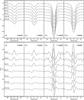 |
Fig. 3 Time series of SVD I (top) and V (bottom) spectra of HD 101412 obtained using different line masks. The profiles are shifted upwards and Stokes V profiles are multiplied by ten for better visibility. From left to right the results correspond to the following line samples: the sample of 650 lines belonging to various iron-peak elements assuming Teff = 8300 K, the sample of 339 Fe i lines (Teff = 8300 K), the sample of 29 Fe i lines assuming Teff = 10 000 K, and the sample of 52 Fe ii lines (Teff = 8300 K). The vertical dashed lines indicate the velocity interval used for the magnetic field measurements. |
In a circumstellar environment, such as a wind or an accretion disk, lines may form over a relatively large volume, and the field topology may be therefore complex not only in latitude and azimuth, but in radius as well. The motion of the CS gas is expected to be governed by the magnetic field, especially in the regions of the stellar wind, which is generally assumed to be accelerated by a magnetic centrifuge. The presence of a clear shift of 4 km s-1 in sharp spectral lines with vsini values of about 3 km s-1 probably indicates the non-photospheric origin of the detected features. As of today, no consistent scenario exists that explains how the magnetic fields in Herbig Ae stars are generated and how they interact with the circumstellar environment. On the other hand, it is probably possible to separate photospheric and CS contributions if very high S/N spectra in the visual and in the near-IR, recorded over the rotation cycle, become available in the future. Spectropolarimetric observations of photospheric lines are usually used to determine the geometry of the global magnetic field, while spectropolarimetry of accretion diagnostic lines (e.g., He i 5876 Å, the Na i doublet, the Balmer lines) probes the accretion topology in accretion columns, which are perturbed by interactions with the disk. The combination of observations in the visual with those in the near-IR appears most useful, since previous near-IR studies of Herbig Ae stars indicate that the He i 1083 nm line is an excellent diagnostic to probe inflow (accretion) and outflow (winds) in the star-disk interaction region (Edwards et al. 2006).
To confirm our suspicion with respect to the impact of the CS contamination, we studied the behaviour of the SVD Stokes V profiles calculated with a second mask, containing 339 neutral iron lines forming at Teff = 8300 K and with a third mask at a significantly higher effective temperature, Teff = 10 000 K containing 29 neutral iron lines. The results are presented in Fig. 3 in the second and the third columns (see also Fig. B.1). Noteworthy, the SVD Stokes V profiles calculated with a mask at a significantly higher effective temperature completely lack distinct features in the red wings of the Zeeman profiles, and show no shifts. Also our analysis of the SVD profiles obtained with a fourth mask containing 52 ionized iron lines presented in the fourth column of Fig. 3 and in Fig. B.1 shows no features in the red wings of the Zeeman profiles, indicating that Fe ii lines are predominantly formed in the stellar photosphere and not in the circumstellar environment. The presented results demonstrate that CS contamination probably plays a role in the appearance of Zeeman features and special care has to be taken in the interpretation of the calculated Stokes V profiles. On the other hand, Zeeman signatures from the first three epochs are much weaker compared to those in the subsequent epochs, with little change in the relative amplitude of the Stokes I profiles. If these signatures are indeed circumstellar in origin, it is not completely clear yet whether we only see the circumstellar contribution during the crossover phases when the Zeeman signature has low amplitude or if this contribution is a time variable phenomenon that happens to be strong enough at the time of the first three epochs of observations and becomes gradually weaker at the subsequent epochs. The measurements using a velocity interval of ± 15 km s-1 are summarized in Table 2.
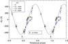 |
Fig. 4 Phase diagram for the longitudinal magnetic field measurements of HD 101412 carried out using low-resolution FORS 2 spectropolarimetric observations (black filled squares) and high-resolution HARPSpol observations. Red open circles represent the SVD measurements via all metallic lines, blue filled circles via Fe i lines at Teff = 8300 K, magenta triangles via Fe ii lines at Teff = 8300 K, and green filled circles via Fe i lines at Teff = 10 000 K. The fit in the plot refers to Hubrig et al. (2011b). |
To visualize our results obtained for the different line masks, we present in Fig. 4 the previously published FORS 2 measurements (Hubrig et al. 2011b) together with our HARPS magnetic field measurements. In this figure, we overplot the results for the samples of Fe i lines at Teff = 8300 K and Teff = 10 000 K, Fe ii lines at Teff = 8300 K, and for the line sample of all metallic lines. The values for the measurements via photospheric Fe i and Fe ii lines appear shifted towards more positive values of the magnetic field strength. This figure also clearly shows that the distribution of field values obtained using HARPSpol spectra is completely different compared to the magnetic field values determined in previous low-resolution FORS 2 measurements, where hydrogen Balmer lines are the main contributors to the magnetic field measurements. This kind of behaviour can likely be explained by the presence of concentration of iron-peak elements in the region of the magnetic equator, similar to the iron peak element spot distribution frequently observed in classical Ap stars (see e.g. Landstreet et al. 2014). The presence of iron spots was already indicated in previous studies of this star by Hubrig et al. (2011b, 2012), who presented variability of equivalent width, radial velocity, line width, and line asymmetry using a sample of blend free iron lines.
3.2. HD 104237
The Herbig Ae star HD 104237 was intensively studied during the last years, in particular, because of the possible presence of a magnetic field announced 16 years ago by Donati et al. (1997). In their work, the authors reported on the probable detection of a weak magnetic field of the order of 50 G. The star is a primary in an SB2 system with an orbital period of 19.86 d (Böhm et al. 2004). A study of the chemical abundances in both components was presented by Cowley et al. (2013). The authors assumed the following fundamental parameters of HD 104237: Teff = 8250 K, log g = 4.2, and v sin i = 8 km s-1, for the primary component, and Teff = 4800 K, log g = 3.7, and v sin i = 12 km s-1, for the secondary. The primary is a δ Scuti-like pulsator with frequencies ranging between 28.5 and 35.6 d-1 (Böhm et al. 2004). The impact of pulsations on the Stokes I profiles is presented in the Appendix.
As a result of the pulsation induced changes detected in the line profiles during the observation, the final Stokes V spectrum is expected to lead to the wrong value for the longitudinal magnetic field. The question of how pulsations affect the magnetic field measurements is not yet solved in spite of the fact that the number of magnetic studies of pulsating stars is gradually increasing. The effect of pulsations on magnetic field measurements was for the first time discussed by Schnerr et al. (2006) and Hubrig et al. (2011a). Schnerr et al. (2006) discussed the influence of pulsations on the analysis of the magnetic field strength in the β Cephei star ν Eri in MUlti-SIte COntinuous Spectroscopy (MUSICOS) spectra and tried to model the signatures found in Stokes V and N spectra. Although the authors reported that they are able to quantitatively establish the influence of pulsations on the magnetic field determination through some modelling, they still detect profiles in Stokes V and N, which are the result of the combined effects of the pulsations and the inaccuracies in wavelength calibration that were not removed by their imperfect modelling of these effects. Hubrig et al. (2011a) suggested carrying out separate measurements of the line shifts between the spectra (I + V)0 and (I − V)0 in the first subexposure and the spectra (I − V)90 and (I + V)90 in the second subexposure (see their Sect. 2 ). The final longitudinal magnetic field value is then calculated as an average of the measurements for each subexposure. We tried to apply a similar procedure to the observations of HD 104237 (see Appendix A.2). However, the very low S/N obtained in the HARPS subexposures did not allow us to draw any conclusions about the strength of the magnetic field.
The results of the measurements of the mean longitudinal magnetic field obtained using the SVD method with 1292 metallic lines in the line mask are presented on the left side of Fig. 5. The polarization feature for the secondary component, which is a T Tauri star, stands out in the SVD Stokes V spectrum corresponding to ⟨Bz⟩ = 129 ± 12 G with FAP < 10-12, from the velocity interval 10–60 km s-1. This is the first registration of the magnetic field in the secondary component of the system HD 104237, and it is in agreement with values derived for some other T Tauri stars (Gregory et al. 2012). If we include an additional few hundred weaker lines in the line mask, we detect in the SVD Stokes V spectrum of the primary a marginal polarization feature at the level of 13 G (right side of Fig. 5). Given the presence of pulsations and the weakness of the detected feature, the presence of the magnetic field in this component remains highly uncertain.
3.3. HD 190073
The absorption and emission spectrum of the Herbig Ae star HD 190073 was studied in detail by Catala et al. (2007) and more recently by Cowley & Hubrig (2012). The low projected rotational velocity (v sin i ≤ 9 km s-1) may indicate either a very slow rotation, or a very small inclination of the rotation axis with respect to the line of sight. Recent interferometric observations in the infrared are best interpreted in terms of a circumstellar disk seen nearly face-on (Eisner et al. 2004). Also IUE observations indicate a low inclination angle of the rotation axis (Hubrig et al. 2009).
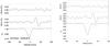 |
Fig. 5 The SVD I, V, and N spectra of HD 104237 obtained with different samples of metallic lines. The dashed lines in the plot on the left side indicate the standard deviations for the N and V spectra. |
The first measurement of a longitudinal magnetic field in HD 190073 was published by Hubrig et al. (2006) indicating the presence of a weak longitudinal magnetic field ⟨Bz⟩ = 84 ± 30 G measured on FORS 1 low-resolution spectra at a 2.8σ level. Later on, this star was studied by Catala et al. (2007) with ESPaDOnS observations, who confirmed the presence of a magnetic field, ⟨Bz⟩ = 74 ± 10 G, at a higher significance level. A longitudinal magnetic field ⟨Bz⟩ = 104 ± 19 G was reported by Hubrig et al. (2009) using FORS 1 measurements. For a number of years, the magnetic field of this star appeared to be rather stable showing positive polarity. More recent observations of this star during 2011 July and 2012 October by Alecian et al. (2013a) with ESPaDOnS and Narval revealed variations of the Zeeman signature in the LSD spectra on timescales of days to weeks. The authors suggested that the detected variations of the Zeeman signatures are the result of the interaction between the fossil field and the ignition of a dynamo field generated in the newly-born convective core. Wade (priv. comm.) stated recently that these results might be due to issues with the instrument or data reduction.
The results of our measurements of the mean longitudinal magnetic field obtained using the SVD method with 287 metallic lines in the line mask for the first epoch on 2011 May 24 are presented on the left side of Fig. 6. At this epoch, we obtain a definite detection ⟨Bz⟩ = −8 ± 6 G with a false alarm probability smaller than 10-8. Both the shape of the profile and the field strength are in agreement with those of Alecian et al. (2013a), who used the same HARPS observations as we did. For the second epoch on 2012 August 7, we achieve a marginal detection ⟨Bz⟩ = −15 ± 10 G with a false alarm probability of 8 × 10⁻⁴. For this epoch, we had to employ 522 metallic lines due to very poor S/N. The resulting mean Stokes I, Stokes V, and null profiles are presented on the right side of Fig. 6. In both cases, the velocity interval used was ± 40 km s-1. The appearance of polarization features, especially on the second epoch in 2012, is not easy to interpret: instead of one Zeeman feature in the SVD Stokes V profile, we detect two Zeeman features of different shapes corresponding to emission wings around the central absorption in the Stokes I profile (see also Fig. 1). This finding may indicate that the CS environment has an impact on the configuration of the magnetic field of HD 190073. No significant fields could be determined from the null spectra, indicating that any noticeable spurious polarization is absent.
4. Discussion
The behaviour of the magnetic field of HD 101412 over the rotation period was previously based only on low-resolution polarimetric spectra. We used high-resolution HARPSpol spectra to investigate the spectral variability on a short timescale and the behaviour of the longitudinal magnetic field over a part of the rotation cycle. Over the time interval covered by the HARPS spectra, the longitudinal magnetic field changes sign from negative to positive polarity. The results of our measurements based on different line samples indicate the presence of differences in the shape of Zeeman features in the Stokes V profiles and in the field strength. For the first time, they are discussed in the context of the impact of the circumstellar matter and elemental abundance inhomogeneities on the measurements of the magnetic field.
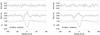 |
Fig. 6 SVD I, V, and N spectra of HD 190073 obtained using a sample of 287 metallic lines at the first epoch and 522 metallic lines at the second epoch.The dashed lines indicate the standard deviations for the N and V spectra. |
In the SVD Stokes V spectrum of HD 104237, we detect a rather strong polarization feature at the position corresponding to the secondary component, which is a T Tauri star. The measured magnetic field is ⟨Bz⟩ = 129 ± 12 G. We only detected a marginal polarization feature at the level of ⟨Bz⟩ = 13 ± 11 G in the Stokes V spectrum of the primary component. Since such SB2 systems with sharp-lined components are extremely rare – no other system with similar spectral characteristics is known to date – it is important to carry out a follow-up study with highly accurate HARPSpol spectra.
Our analysis of HD 190073 confirms the presence of a variable magnetic field. The shape of the detected polarization features indicates a significant contribution of the CS environment in this star. Polarimetric spectra at higher S/N are urgently needed to understand the magnetic field topology.
Magnetospheric accretion has been well established for T Tauri stars and depends on a strong ordered predominantly dipolar field channelling circumstellar disk material to the stellar surface via accretion streams. To properly understand the magnetospheres of Herbig Ae stars and their interaction with the circumstellar environment presenting a combination of disk, wind, accretion, and jets, knowledge of the magnetic field strength and topology is indispensable. Progress in understanding the disk-magnetosphere interaction can, however, only come from studying a sufficient number of targets in detail to look for patterns encompassing Herbig Ae stars.
Online material
Appendix A: The study of spectral variability on short timescales
Given the rather low S/N of the HARPS spectra, to study the spectral variability on short timescales, we employed the LSD technique, allowing us to achieve much higher S/N in the LSD spectra. The details of this technique can be found in the work of Donati et al. (1997). The line masks are constructed using the VALD database (e.g. Kupka et al. 2000). As mentioned in Sect. 3, the reconstruction of the intensity profile (Stokes I) does not need the generally time-consuming application of the SVD technique.
Appendix A.1: HD 101412
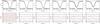 |
Fig. A.1 Top panel: comparison of the LSD Stokes I profiles of HD 101412 computed for individual subexposures recorded over six observing nights in 2014 February using the line mask of 1007 metallic lines. Eight individual subexposures were obtained during the first night, while four subexposures were obtained for each following night. Bottom panel: differences between Stokes I profiles computed for the individual subexposures and the average Stokes I profile. The dashed lines indicate the standard deviation limits. |
Seven spectropolarimetric observations were obtained with the HARPS polarimeter on the nights from 2013 February 14 to 21. Among them, two individual observations have been obtained during the first night on February 14. Each observation was split into four subexposures with an exposure time of 10–12 min, obtained with different orientations of the quarter-wave retarder plate relative to the polarization beam splitter of the circular polarimeter. In Fig. A.1, we present the comparison between the LSD Stokes I profiles computed for each individual subexposure recorded on the six different nights. The results for both observations obtained on the first night on February 14, each consisting of four subexposures, are presented in the same panel. No significant variation in the line profile or radial velocity is detected in the behaviour of the Stokes I profiles for each subexposure. Signal-to-noise values achieved in the spectra observed during the last three observing nights are in the range from 76 to 58, i.e. significantly lower than those achieved in the first three epochs. For these last three nights, we observe very tiny changes in the cores and wings of the overplotted LSD Stokes I profiles with an intensity variation of the order of the spectral noise of about 0.3%.
Appendix A.2: HD 104237
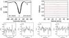 |
Fig. A.2 Upper row: comparison of the LSD Stokes I profiles of HD 104237 computed for the individual subexposures obtained with a time lapse of 2.2 min (left side) and differences between Stokes I profiles computed for the individual subexposures and the average Stokes I profile with standard deviation limits indicated by the dashed lines (right side). Lower row: Stokes V spectra calculated for the combination of pairs of two subexposures with the quarter-wave plate angles separated by 90 degrees, four pairs in all. |
The primary is a δ Scuti-like pulsator with frequencies ranging between 28.5 and 35.6 d-1 (Böhm et al. 2004). The observation on 2010 May 3 was split into eight subexposures with an exposure time of 2.2 min. The line mask included 1007 metallic lines. In Fig. A.2 in the upper row, we present the impact of
pulsations on the Stokes I profiles computed for each individual subexposure. Because of the pulsation changes in the line profiles during the observation, the final Stokes V spectrum is expected to lead to a wrong value of the longitudinal magnetic field. To prove whether the primary possesses a field, we used pairs of two subexposures with the quarter-wave plate angles separated by 90 degrees, four pairs in all. However, no conclusions about the presence of a magnetic field in this component can be drawn due to the very low S/N achieved. The computed Stokes V spectra for each pair of subexposures are presented in the lower row of Fig. A.2.
Appendix A.3: HD 190073
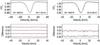 |
Fig. A.3 Comparison of the LSD Stokes I profiles of HD 190073 computed for the individual subexposures obtained on 2011 May 24 with a time lapse of about 10 min (left panel) and on 2012 August 7 with a time lapse of 30 min (right panel). The dashed lines on the lower plots indicate the standard deviation limits. |
This star was not reported in the literature to show δ Scuti-like pulsations. The line mask in our analysis included 375 metallic lines. The inspection of the behaviour of the LSD Stokes I profiles presented in Fig. A.3 calculated for each subexposure does not reveal any line profile or radial velocity variation on a timescale of about ten minutes during the first epoch in 2011 or on a timescale of 30 minutes during the second epoch in 2012.
Appendix B: The SVD profiles
 |
Fig. B.1 Correspondence of SVD I and V profiles of HD 101412 obtained using different line masks. From left to right the results correspond to the following line samples: the sample of 650 lines belonging to various iron-peak elements assuming Teff = 8300 K, the sample of 339 Fe i lines (Teff = 8300 K), the sample of 29 Fe i lines assuming Teff = 10 000 K, and the sample of 52 Fe ii lines (Teff = 8300 K). The time runs from bottom to top. |
Acknowledgments
We thank the anonymous referee for valuable comments. S.P.J. acknowledges support from Deutsche Forschungsgemeinschaft, DFG project number JA 2499/1–1. N.A.D. thanks Saint Petersburg State University, Russia, for research grant 6.38.18.2014 and FAPERJ, Rio de Janeiro, Brazil, for Visiting Researcher grant E-26/200.128/2015.
References
- Alecian, E., Neiner, C., Mathis, S., et al. 2013a, A&A, 549, L8 [NASA ADS] [CrossRef] [EDP Sciences] [Google Scholar]
- Alecian, E., Wade, G. A., Catala, C., et al. 2013b, MNRAS, 429, 1001 [NASA ADS] [CrossRef] [Google Scholar]
- Barnes, J. R. 2004, MNRAS, 348, 1295 [Google Scholar]
- Böhm, T., Catala, C., Balona, L., & Carter, B. 2004, A&A, 427, 907 [NASA ADS] [CrossRef] [EDP Sciences] [Google Scholar]
- Carroll, T. A., Strassmeier, K. G., Rice, J. B., & Künstler, A. 2012, A&A, 548, A95 [NASA ADS] [CrossRef] [EDP Sciences] [Google Scholar]
- Catala, C., Alecian, E., Donati, J.-F., et al. 2007, A&A, 462, 293 [NASA ADS] [CrossRef] [EDP Sciences] [Google Scholar]
- Cowley, C. R. & Hubrig, S. 2012, Astron. Nachr., 333, 34 [NASA ADS] [CrossRef] [Google Scholar]
- Cowley, C. R., Hubrig, S., González, J. F., & Savanov, I. 2010, A&A, 523, A65 [NASA ADS] [CrossRef] [EDP Sciences] [Google Scholar]
- Cowley, C. R., Castelli, F., & Hubrig, S. 2013, MNRAS, 431, 3485 [NASA ADS] [CrossRef] [Google Scholar]
- Donati, J.-F., Semel, M., & Rees, D. E. 1992, A&A, 265, 669 [NASA ADS] [Google Scholar]
- Donati, J.-F., Semel, M., Carter, B. D., Rees, D. E., & Collier Cameron, A. 1997, MNRAS, 291, 658 [NASA ADS] [CrossRef] [MathSciNet] [Google Scholar]
- Donati, J.-F., Gregory, S. G., Montmerle, T., et al. 2011, MNRAS, 417, 1747 [NASA ADS] [CrossRef] [Google Scholar]
- Edwards, S., Fischer, W., Hillenbrand, L., & Kwan, J. 2006, ApJ, 646, 319 [NASA ADS] [CrossRef] [Google Scholar]
- Eisner, J. A., Lane, B. F., Hillenbrand, L. A., Akeson, R. L., & Sargent, A. I. 2004, ApJ, 613, 1049 [NASA ADS] [CrossRef] [Google Scholar]
- Gregory, S. G., Donati, J.-F., Morin, J., et al. 2012, ApJ, 755, 97 [NASA ADS] [CrossRef] [Google Scholar]
- Hubrig, S., Yudin, R. V., Schöller, M., & Pogodin, M. A. 2006, A&A, 446, 1089 [NASA ADS] [CrossRef] [EDP Sciences] [Google Scholar]
- Hubrig, S., Stelzer, B., Schöller, M., et al. 2009, A&A, 502, 283 [NASA ADS] [CrossRef] [EDP Sciences] [Google Scholar]
- Hubrig, S., Schöller, M., Savanov, I., et al. 2010, Astron. Nachr., 331, 361 [NASA ADS] [CrossRef] [Google Scholar]
- Hubrig, S., Ilyin, I., Briquet, M., et al. 2011a, A&A, 531, L20 [NASA ADS] [CrossRef] [EDP Sciences] [Google Scholar]
- Hubrig, S., Mikulášek, Z., González, J. F., et al. 2011b, A&A, 525, L4 [NASA ADS] [CrossRef] [EDP Sciences] [Google Scholar]
- Hubrig, S., Castelli, F., González, J. F., et al. 2012, A&A, 542, A31 [NASA ADS] [CrossRef] [EDP Sciences] [Google Scholar]
- Hubrig, S., Ilyin, I., Schöller, M., & Lo Curto, G. 2013, Astron. Nachr., 334, 1093 [NASA ADS] [CrossRef] [Google Scholar]
- Hubrig, S., Carroll, T. A., González, J. F., et al. 2014, MNRAS, 440, L6 [NASA ADS] [CrossRef] [Google Scholar]
- Hubrig, S., Carroll, T. A., Schöller, M., & Ilyin, I. 2015, MNRAS, 449, L118 [NASA ADS] [CrossRef] [Google Scholar]
- Kallinger, T., Zwintz, K., & Weiss, W. 2008, A&A, 488, 279 [NASA ADS] [CrossRef] [EDP Sciences] [Google Scholar]
- Kupka, F. G., Ryabchikova, T. A., Piskunov, N. E., Stempels, H. C., & Weiss, W. W. 2000, Balt. Astron., 9, 590 [NASA ADS] [Google Scholar]
- Landstreet, J. D., Bagnulo, S., & Fossati, L. 2014, A&A, 572, A113 [NASA ADS] [CrossRef] [EDP Sciences] [Google Scholar]
- Li, H.-B., Dowell, C. D., Goodman, A., Hildebrand, R., & Novak, G. 2009, ApJ, 704, 891 [NASA ADS] [CrossRef] [Google Scholar]
- Mathys, G. 1989, Fund. Cosmic Phys., 13, 143 [Google Scholar]
- Rucinski, S. M. 1992, AJ, 104, 1968 [NASA ADS] [CrossRef] [Google Scholar]
- Rucinski, S. M., Lu, W.-X., & Shi, J. 1993, AJ, 106, 1174 [NASA ADS] [CrossRef] [Google Scholar]
- Schnerr, R. S., Verdugo, E., Henrichs, H. F., & Neiner, C. 2006, A&A, 452, 969 [NASA ADS] [CrossRef] [EDP Sciences] [Google Scholar]
- Snik, F., Jeffers, S., Keller, C., et al. 2008, in SPIE Conf. Ser., 7014, 70140O [Google Scholar]
- Wade, G. A., Drouin, D., Bagnulo, S., et al. 2005, A&A, 442, L31 [NASA ADS] [CrossRef] [EDP Sciences] [Google Scholar]
- Wade, G. A., Bagnulo, S., Drouin, D., Landstreet, J. D., & Monin, D. 2007, MNRAS, 376, 1145 [NASA ADS] [CrossRef] [MathSciNet] [Google Scholar]
- Waite, I. A., Marsden, S. C., Carter, B. D., et al. 2015, MNRAS, 449, 8 [NASA ADS] [CrossRef] [Google Scholar]
All Tables
For each sample, the signal-to-noise ratio achieved in the SVD spectra and the measured longitudinal magnetic field are presented. The average Landé factor used in the SVD measurements is also indicated.
All Figures
|
Fig. 1 Example spectra of the three sharp-lined Herbig Ae stars HD 101412, HD 104237, and HD 190073. |
| In the text | |
|
Fig. 2 The correspondence of SVD I, V, and N profiles of HD 101412 obtained using a sample of 650 lines belonging to various iron-peak elements assuming Teff = 8300 K. The profiles obtained using other line samples are presented in Fig. B.1. |
| In the text | |
|
Fig. 3 Time series of SVD I (top) and V (bottom) spectra of HD 101412 obtained using different line masks. The profiles are shifted upwards and Stokes V profiles are multiplied by ten for better visibility. From left to right the results correspond to the following line samples: the sample of 650 lines belonging to various iron-peak elements assuming Teff = 8300 K, the sample of 339 Fe i lines (Teff = 8300 K), the sample of 29 Fe i lines assuming Teff = 10 000 K, and the sample of 52 Fe ii lines (Teff = 8300 K). The vertical dashed lines indicate the velocity interval used for the magnetic field measurements. |
| In the text | |
|
Fig. 4 Phase diagram for the longitudinal magnetic field measurements of HD 101412 carried out using low-resolution FORS 2 spectropolarimetric observations (black filled squares) and high-resolution HARPSpol observations. Red open circles represent the SVD measurements via all metallic lines, blue filled circles via Fe i lines at Teff = 8300 K, magenta triangles via Fe ii lines at Teff = 8300 K, and green filled circles via Fe i lines at Teff = 10 000 K. The fit in the plot refers to Hubrig et al. (2011b). |
| In the text | |
|
Fig. 5 The SVD I, V, and N spectra of HD 104237 obtained with different samples of metallic lines. The dashed lines in the plot on the left side indicate the standard deviations for the N and V spectra. |
| In the text | |
|
Fig. 6 SVD I, V, and N spectra of HD 190073 obtained using a sample of 287 metallic lines at the first epoch and 522 metallic lines at the second epoch.The dashed lines indicate the standard deviations for the N and V spectra. |
| In the text | |
|
Fig. A.1 Top panel: comparison of the LSD Stokes I profiles of HD 101412 computed for individual subexposures recorded over six observing nights in 2014 February using the line mask of 1007 metallic lines. Eight individual subexposures were obtained during the first night, while four subexposures were obtained for each following night. Bottom panel: differences between Stokes I profiles computed for the individual subexposures and the average Stokes I profile. The dashed lines indicate the standard deviation limits. |
| In the text | |
|
Fig. A.2 Upper row: comparison of the LSD Stokes I profiles of HD 104237 computed for the individual subexposures obtained with a time lapse of 2.2 min (left side) and differences between Stokes I profiles computed for the individual subexposures and the average Stokes I profile with standard deviation limits indicated by the dashed lines (right side). Lower row: Stokes V spectra calculated for the combination of pairs of two subexposures with the quarter-wave plate angles separated by 90 degrees, four pairs in all. |
| In the text | |
|
Fig. A.3 Comparison of the LSD Stokes I profiles of HD 190073 computed for the individual subexposures obtained on 2011 May 24 with a time lapse of about 10 min (left panel) and on 2012 August 7 with a time lapse of 30 min (right panel). The dashed lines on the lower plots indicate the standard deviation limits. |
| In the text | |
|
Fig. B.1 Correspondence of SVD I and V profiles of HD 101412 obtained using different line masks. From left to right the results correspond to the following line samples: the sample of 650 lines belonging to various iron-peak elements assuming Teff = 8300 K, the sample of 339 Fe i lines (Teff = 8300 K), the sample of 29 Fe i lines assuming Teff = 10 000 K, and the sample of 52 Fe ii lines (Teff = 8300 K). The time runs from bottom to top. |
| In the text | |
Current usage metrics show cumulative count of Article Views (full-text article views including HTML views, PDF and ePub downloads, according to the available data) and Abstracts Views on Vision4Press platform.
Data correspond to usage on the plateform after 2015. The current usage metrics is available 48-96 hours after online publication and is updated daily on week days.
Initial download of the metrics may take a while.