| Issue |
A&A
Volume 583, November 2015
|
|
|---|---|---|
| Article Number | A109 | |
| Number of page(s) | 9 | |
| Section | The Sun | |
| DOI | https://doi.org/10.1051/0004-6361/201526912 | |
| Published online | 02 November 2015 | |
Heating and cooling of coronal loops observed by SDO⋆
1
Key Laboratory of Solar Activity, National Astronomical Observatories,
Chinese Academy of Sciences, 100012
Beijing, PR China
e-mail: This email address is being protected from spambots. You need JavaScript enabled to view it.
2
Max Planck Institute for Solar System Research
(MPS), 37077
Göttingen,
Germany
Received: 8 July 2015
Accepted: 14 September 2015
Abstract
Context. One of the most prominent processes to have been suggested as heating the corona to well above 106 K builds on nanoflares, which are short bursts of energy dissipation.
Aims. We compare observations to model predictions to test the validity of the nanoflare process.
Methods. Using extreme UV data from AIA/SDO and HMI/SDO line-of-sight magnetograms, we study the spatial and temporal evolution of a set of loops in active region AR 11850.
Results. We find a transient brightening of loops in emission from Fe xviii forming at about 7.2 MK, while at the same time these loops dim in emission from lower temperatures. This points to a fast heating of the loop that goes along with evaporation of material that we observe as apparent upward motions in the image sequence. After this initial phase lasting some 10 min, the loops brighten in a sequence of AIA channels that show progressively cooler plasma, indicating that this cooling of the loops lasts about one hour. A comparison to the predictions from a 1D loop model shows that this observation supports the nanoflare process in (almost) all aspects. In addition, our observations show that the loops get broader while getting brighter, which cannot be understood in a 1D model.
Key words: Sun: corona / Sun: UV radiation / Sun: atmosphere / Sun: activity
Movie associated to Fig. 1 is available in electronic form at http://www.aanda.org
© ESO, 2015
1. Introduction
How structures in the upper solar atmosphere, i.e. the transition region and corona, are heated and sustained is one of the major unresolved issues in solar and stellar astrophysics (e.g., Klimchuk 2006). Active regions (ARs) that are dominated by loops, which are prominently seen in extreme ultraviolet (EUV) and X-rays, are the ideal place to investigate the dominant heating mechanism(s) in the upper solar atmosphere. The AR loops constitute basic building blocks and are usually divided into two types: warm loops (~1 MK, Ugarte-Urra et al. 2009) and hot loops (>2 MK, Antiochos et al. 2003). These have been vastly studied in theory and observations for understanding the coronal heating (see a review in Klimchuk 2006).
The processes that provide the energy input for the loops can be categorized into two classes: steady heating (Reale et al. 2000; Antiochos et al. 2003; Brooks & Warren 2009) and impulsive heating (Warren 2003; Patsourakos & Klimchuk 2006; Feng & Gan 2006; Tripathi et al. 2010). In general, they can be distinguished by comparing the time scale of the heat input with the typical coronal cooling time, which is about (a fraction of) an hour. If there are separate pulses of heating that are shorter than the cooling time, the heating is considered impulsive. Steady heating will also be found if the energy input lasts for much longer than the cooling time (or if many very short pulses come in rapid succession, so that the corona has no time between the short pulses to relax). Evidence of both steady and impulsive heating are found in coronal observations. However, from 3D magnetohydrodynamics (MHD) modeling, this distinction of steady and impulsive heating for loops is not that clear. Such models show that even on the same fieldline on one leg, the heating can be steady, while it is impulsive on the other leg (Bingert & Peter 2011; Peter 2015).
By studying an AR moss area, i.e. footpoints of hot loops, Antiochos et al. (2003) suggest that the heating is quasi-steady. Brooks & Warren (2009) and Dadashi et al. (2012) analyzed the Doppler shifts of an AR moss and also find support for quasi-steady heating. In contrast, Klimchuk (2006) argues that most coronal heating mechanisms are impulsive for elemental magnetic flux strands within a loop. Nanoflares, as proposed by Parker (1972; 1988), are usually considered to be the source of impulsive heating in these strands, and a coronal loop is considered to be a bundle of unresolved strands (Cargill 1994). Observational arguments have been put forward that these fundamental strands have to have sizes of 500 km (Brooks et al. 2012, 2013) or even less (Peter et al. 2013). Tripathi et al. (2010) compared the observed and theoretical emission measure distributions in an AR core and propose that the hot loops are heated by nanoflares. Using imaging in six different channels in the EUV, Viall & Klimchuk (2012) analyzed the lightcurves of coronal loops. By comparing with theoretical models, they suggest that loops both in and surrounding the AR cores are heated by impulsive nanoflares. By measuring the Doppler shifts in AR moss in lower temperature lines, Winebarger et al. (2013) provide strong evidence that hot loops are impulsively heated. Recently, Ugarte-Urra & Warren (2014) have investigated the frequency of transient brightenings in an AR core and find that there are nearly two to three heating events per hour.
Once the heating has cease, the bundle of loop strands cools down. The lightcurves of coronal loops of channels or spectral lines showing cooler plasma reach their peaks at progressively later times than channels showing hotter plasma (Schrijver 2001; Warren et al. 2002; Müller et al. 2004; Peter et al. 2012). This time lag has been interpreted as the result of hot coronal loop plasma cooling down. Using data from the EUV Imaging Spectrometer (EIS) onboard Hinode, Ugarte-Urra et al. (2009) could follow the cooling of loops down to transition region temperatures after a heat deposition. Viall & Klimchuk (2012) observe that there is a time lag that is consistent with cooling plasma not only for loops throughout an AR, but also for the diffuse emission between the loops. Alissandrakis & Patsourakos (2013) identified some loops that were initially visible in the AIA 94 Å images, subsequently in the AIA 335 Å, and in one case in the AIA 211 Å channels, supporting the cooling of impulsive heated loops. However, with the interpretation of this and other AIA data sets, one has to consider that they are naturally multi-thermal because they cover a broad range of temperatures (e.g., Del Zanna et al. 2011). Attention should be paid to the interpretation of the AIA observed features that can be affected by the contribution of particular spectral lines under certain conditions (e.g., O’Dwyer et al. 2010).
High-speed evaporative upflows reaching speeds of more than 100 km s-1 are predicted by 1D loop models with a prescribed impulsive heat input as expected for, e.g., nanoflares (Antiochos & Sturrock 1979; Patsourakos & Klimchuk 2006). Although at somewhat slower speeds of just below 100 km s-1, these upflows are also found in a 3D MHD model of an emerging AR (Chen et al. 2014). De Pontieu et al. (2009) looked at the asymmetry of line profiles and concluded that the line asymmetry is caused by a high-velocity upflow at the loop footpoint (Tian et al. 2011; Doschek 2012), but this is interpreted by others as propagating slow magneto-acoustic waves (Gupta et al. 2012) or as being dominated by uncertainties (Tripathi & Klimchuk 2013). Dadashi et al. (2012) find that the inner part of a moss area shows a blueshift of 5 km s-1 for cooler lines (1.0–1.6 MK) and 1 km s-1 for hotter lines (~2 MK). Tripathi et al. (2012) present observations of upflows in warm loops (0.6–1.6 MK) with speeds decreasing with height and considered them to be evidence of chromospheric evaporative upflows. Orange et al. (2013) studied a catastrophically cooling loop and observed the plasma upflows at its footpoint sites at multiple transition region temperatures. On the other hand, downflows are expected during the cooling process owing to the heated plasma radiatively cooling and condensing in the loops. Redshifts have been reported previously at footpoints and along the loop structures, thereby supporting the presence of cooling downflows (Del Zanna 2008; Tripathi et al. 2009). Cool plasma sliding down on both sides of coronal loop with speeds of up to 100 km s-1 are also reported by Schrijver (2001) and has been modeled by Müller et al. (2005). Moreover, Ugarte-Urra et al. (2009) detected cooling downflows with velocities in the range of 40 km s-1 to over 105 km s-1.
To test the nanoflare model for coronal heating, in particular with respect to the 1D models of Patsourakos & Klimchuk (2006), we chose a set of AR loops observed by the Atmospheric Imaging Assembly (AIA; Lemen et al. 2012) onboard the Solar Dynamics Observatory (SDO; Pesnell et al. 2012). We investigate the evolution of heated and cooling loops in detail and compare these observations with theoretical models. This shows clear evidence of nanoflare heating of coronal loops for at least this set of observed loops.
2. Observations and data processing
The AIA instrument consists of a set of normal incidence EUV telescopes designed for acquiring solar atmospheric images at ten wavelength bands. In this study, we use AIA multiwavelength images from September 24, 2013 with a time cadence and spatial sampling of 12 s and 0.6 ′′/pixel to study the evolution of AR loops. Line-of-sight magnetograms from the Helioseismic and Magnetic Imager (HMI; Schou et al. 2012) onboard SDO were used to investigate the underlying photospheric magnetic field. The spatial sampling and time cadence of the HMI data are 0.5 ′′/pixel and 45 s, respectively.
To analyze the evolution of the hot plasma in the loops, the contribution of the Fe XVIII
emission line was isolated from the AIA 94 Å images using the empirical method devised by
Warren et al. (2012). This is to avoid contamination
from the cooler plasma (mostly around 1 MK) that also contributes to this channel (Boerner
at al. 2012). According to ionization equilibrium, the
Fe XVIII line shows plasma around 7.2 MK. Following Ugarte-Urra & Warren (2014), the Fe XVIII images were obtained from the AIA
94 Å images by subtracting the contaminating warm (i.e., around 1 MK) component to the
bandpass. This warm contribution was computed from a weighted combination of the emission
from the AIA 171 Å and 193 Å channels dominated by Fe X and Fe XII emission, respectively.
This empirical isolation can be expressed as 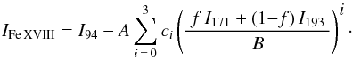 (1)Here the weighting is given by c = [−7.19 × 10⁻²,
9.75 × 10⁻¹,
9.79 × 10⁻²,
−2.81 × 10⁻³], and
A = 0.39,
B = 116.32,
f = 0.31.
More details are found in Warren et al. (2012) and
Ugarte-Urra & Warren (2014).
(1)Here the weighting is given by c = [−7.19 × 10⁻²,
9.75 × 10⁻¹,
9.79 × 10⁻²,
−2.81 × 10⁻³], and
A = 0.39,
B = 116.32,
f = 0.31.
More details are found in Warren et al. (2012) and
Ugarte-Urra & Warren (2014).
3. Heating of loops
On September 24, 2013 the AR NOAA AR 11850 was observed by SDO at the heliographic position N10 E20. From 03:00 UT to 05:00 UT a set of loops was located to the northerm end of the AR. Most importantly, no other loop structures were detected surrounding these loops, so that it is possible to study an isolated set of loops. These were heated and subsequently cooled down. First they showed signatures of brightening (Sect. 3.1) and plasma injection (Sect. 3.2) in Fe XVIII originating in hot (heated) plasma, together with a dimming in cooler channels (Sect. 3.3). After some time, evidence of cooling is observed (Sect. 4).
3.1. Brightening of a hot loop in Fe XVIII
Figure 1 displays the general information on the loops in the AIA multiwavelength observation, together with the information on the magnetic field from HMI. Each coronal band is shown when Loop 1 is close to its peak brightness (dotted lines in Fig. 2 for each of the bands), spanning roughly one hour. The HMI magnetogram is taken around the middle of that time interval. The Fe XVIII loop consists of two components, a northern thick loop, Loop 1, and a southern thin loop, Loop 2. In this paper, we primarily study the northern main loop, Loop 1. It first appears in the Fe XVIII images at about 03:20 UT with a length of nearly 70 Mm. Moreover, around this time, there is no corresponding loop visible in other AIA channels (see movie attached to Fig. 1). On the one hand this indicates that the loops are heated up the Fe XVIII line characteristic temperature of ~7.2 MK, because they are not seen in the cooler channels. On the other hand, the loop is not heated to temperatures much higher than about 7 MK, because otherwise it should be visible in the 131 Å channel that receives a significant contribution from plasma at around 10 MK (often seen in flares).
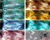 |
Fig. 1 AIA/SDO extreme UV images and HMI/SDO magnetogram. Panels (a)–g)) display the loops as seen in Fe XVIII a), AIA 94 Å b), 335 Å c), 211 Å d), 193 Å e), 171 Å f), and 131 Å g). Panel h) shows the line-of-sight magnetogram. The Fe XVIII image is derived from the AIA images. (see Eq. (1)). The arrows point to the two loops investigated here. Each of the images (a)–g)) is shown when the loops become clearly visible in the respective band. The blue circles mark the footpoints of the loops, and the blue rectangles in (a)–g)) the regions for the lightcurves of the Loop 1, as shown in Figs. 2 and 5. The white rectangles NS in (a), c)–g)) indicate the positions for the time-space diagrams displayed in Fig. 3. The red rectangle EW in a), the red line EW in f), and the black rectangles EW in (c)–g)) show the positions for space-time diagrams displayed in Figs. 4a, b, and 7, respectively. E, W, N, and S separately denote the heliographic directions. The field of view (FOV) is 150″× 60″. (An animation of this figure is available online.) |
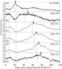 |
Fig. 2 Lightcurves of Loop1. The channels are denoted with the plots. The emission is integrated over the region marked by the blue rectangles indicated in Fig. 1. The lightcurve in the AIA 94 Å channel (not shown) is essentially the same as for the Fe XVIII line. The dotted lines indicate the times when the loop 1 became clearly evident in the respective AIA channel as shown in Figs. 1a–g. The arrows point to the respective peaks of these lightcurves. The dashed lines indicate the time interval shown in Fig. 5. |
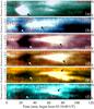 |
Fig. 3 Brightening of Loop 1. The panels show the time-space diagrams along the NS direction in the white rectangles in Fig. 1. Here the distance is across the loop. The black arrows point to Loop 1, and the white arrows the dimming. The dotted lines outline the brightening expanding perpendicular to the loop, and the dashed lines the dimming as it expands. The respective mean velocities are denoted by the numbers in the plots. N and S are the same as in Fig. 1. |
Three blue circles mark the footpoints of the two loops, among which the western one encircles the two neighboring western footpoints of Loops 1 and 2. To show the relation to the magnetic field, we overlay them on the line-of-sight magnetogram (Fig. 1h): the two loops separately connect two plage-type areas of the AR with opposite polarities.
To determine the overall change in intensity of Loop 1, we integrated the emission of Fe XVIII (blue rectangle in Fig. 1a). The resulting (normalized) lightcurve is then shown in Fig. 2a. (The lightcurve in the AIA 94 Å channel shows a similar trend.) Fe XVIII quickly increases in brightness then decreases again, with the whole brightening of the loop lasting ~25 min.
This brightening loop is quite thin when it first appears and then gets broader (i.e., increases its cross section) over the course of 10 min reaches a width of almost ~8′′ (discussed further in Sect. 5.4). This is illustrated in Fig. 3, where we show space-time plots of the evolution of the emission across the loops. For this we integrate the emission in the white rectangle labeled NS in Fig. 1 in the east-west direction, i.e. along the loop. For each image of the time series, this provides an average variation in the intensity across the loop. This average variation across the loop is then plotted in Fig. 3 as a function of time for each of the observed channels. Panel a of Fig. 3 shows the space-time plot for Fe XVIII. Here Loop 1 (black arrow) first brightens in the middle and then gradually expands to both sides (red dotted lines). The propagation of the brightening expands with about 5 km s-1 to 10 km s-1 across the loop, respectively.
Comparison with models will have to show whether this motion is a real motion of the plasma due to an expansion of the loop. Another option would be that the fieldlines farther away from the center of the loop get heated (and brighten) a bit later than the fieldlines in the center, as one expects from 3D MHD models of loops forming in an emerging AR (Chen et al. 2014; 2015).
3.2. Motions along hot loop in Fe XVIII
To investigate the motions along the loops, we created time-space plots similar to the ones above, but now showing the (average) variation along the loop (roughly in the east-west direction). For this we integrated the intensity (red rectangle in Fig. 1a) along the north-south direction and then plot this average versus time. This is shown for Fe XVIII along Loop 1 in Fig. 4a.
At both footpoints we see upward proper motions along the loop. The upflow at both feet start at almost at the same time (~03:28 UT) and move with about 40 km s-1 at the eastern footpoint and almost 100 km s-1 at the western one. This proper motion could be a propagation front of enhanced emission due to increasing temperature and/or a signature of an actual evaporative plasma flow into the loop in response to increased heating.
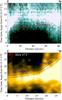 |
Fig. 4 Proper motions along the loops. The panels show the space-time plots of the Fe XVIII a) and AIA 171 Å b) images along the direction EW in the red rectangle in Fig. 1a and the red line EW in Fig. 1f. In contrast to Fig. 3, here the distance is along the loop. The red dotted and dashed lines in a) and the blue dash-dotted and solid lines in b) indicate the proper motions. The mean speeds are denoted by the numbers in the plots. E and W are the same as in Fig. 1. |
Properties of the AIA/SDO multiwavelength loop and comparison to the nanoflare model.
3.3. Dimming in cooler channels
Almost simultaneous with the appearance of the Fe XVIII loops, a dimming takes place in the AIA channels’ imaging cooler plasma (<7 MK), as is clearest in the lightcurves of Fig. 2. This dimming is also clearly visible in the images and difference images as shown in Fig. 6. The overlay of the brightening in Fe XVIII as a contour on top of the base difference images (Figs. 6d–f) makes it clear that the dimming in the cool channels is not only cotemporal with the brightening in Fe XVIII showing the hot plasma, but that it is also cospatial.
To highlight the very close timing of the brightening of the hot and the dimming of the cool plasma, we overplot normalized curves for the loop brightness in Fig. 5. Here the cool channels (335 Å, 211 Å, 193 Å, 171 Å, and 131 Å) are all normalized to the average intensity before the event. For the hot plasma we plot I = 1.0 − IFe XVIII, where IFe XVIII is the Fe XVIII normalized to before the event. All the lightcurves have the same shape falling remarkably well on top of each other. This underlines that the dimming is really cotemporal with the brightening of the Fe XVIII loop.
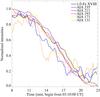 |
Fig. 5 Similar to Fig. 2, but for the time range between two dashed lines as indicated in Fig. 2. All the lightcurves are normalized. In the case of Fe xviii, we show the inverse of the lightcurve to make clear that the cool channels get dark in synchrony with Fe xviii getting bright. |
Similarly as for Fe XVIII we check a space-time plot to investigate the evolution of the dimming in the cool channels across the loop (Figs. 3b–f). Similar to the brightening in Fe XVIII, all the cool channels show consistent expansion across the loop with a speed in the range of 5 km s-1 to 10 km s-1 that is cospatial and cotemporal.
From this we conclude that the dimming of the cool channels is indeed correlated exactly with the brightening of the hot plasma. This provides strong observational support that the loop under investigation was quickly heated to some 7 MK.
4. Cooling of loops
After the brightening in the Fe XVIII line in response to heating (Sect. 3), the loop subsequently brightens in bands showing cooler plasma (Sect. 4.1) and shows signs of plasma draining (Sect. 4.2) in response to cooling.
4.1. Loop brightening in cooler channels
Figures 1c–g show the loop subsequently in the cooler channels of AIA. We show the snapshots at times when the loops are clearly visible and indicate these times in the lightcurves shown in Figs. 2b–f (dotted lines). Similar to the Fe XVIII loops shown in Fig. 1a, the loops in the cooler channels also consist of two subloops, Loops 1 and 2. Their footpoints are located at the same positions as those of the Fe XVIII loops, indicated in Figs. 1c–g (blue circles). Furthermore, the loops are definitely not detected in AIA 304 Å channel, which shows emission at around 0.1 MK. This is cooler than for the AIA 131 Å channel, suggesting that the loops are cooling down to, but not much lower than, ~0.6 MK, which is temperature of the maximum contribution of the AIA 131 Å channel.
Figures 2b–f displays the lightcurves of Loop 1 in the cooler channels of AIA. They show that the loop begins to brighten after the initial dimming. The arrows in Fig. 2 indicate the peak times of the loop intensities in the respective channels. The gradual cooling is clearly discernible through the peak times of the brightening according to the temperature of maximum contribution. The beginning and peak times of the AIA channels are listed in Table 1. One can easily identify the time delay of the loop brightening in different wavelength bands during the cooling process.
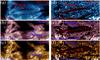 |
Fig. 6 AIA/SDO extreme UV images and corresponding base-difference images. Panels (a)–c)) show the original images and panels (d)–f)) the respective difference images (d)–f)). The red contours in (d)–f)) indicate the Fe XVIII loops in Fig. 1a. Same FOV as in Fig. 1. |
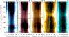 |
Fig. 7 Proper motions along the loop. Similar to Fig. 4, but along the EW direction in the black rectangles in Loop 1 in Figs. 1c–g. The red dotted and dashed lines indicate upward and downward proper motions near the loop footpoints. The respective mean velocities are denoted by the numbers in the plots. The black dash-dotted lines indicate when the loop first becomes visible in the respective channel (same times as in Fig. 2). E and W are the same as in Fig. 1. |
Figures 3b–f illustrate the evolution of the brightening of loop 1 in the cooler channels after time ~30 min (black arrows). These show space-time plots, where the variation across the loop is averaged along the NS direction in the white rectangles shown in Fig. 1. Similar to the initial brightening of the Fe XVIII loop in Fig. 3a, in the cooler channels the loops begin to brighten also in the middle, and then this brightening propagates to both sides, as indicated in Figs. 3b–f (dotted lines; see further discussion in Sect. 5.4). Here the propagation is in the range of 1 km s-1 to 3 km s-1, so smaller than in the case of the Fe XVIII loop. The gradual appearance of the loop is slightly different in the different wavelength channels. Moreover, the loop appears about 1′′ to the north of the Fe XVIII loop for the AIA 335 Å channel and about 2′′ for other AIA cooler channels. This offset is most likely due to a slow (~1 km s-1) transversal motion of the loop. This is also supported by the offset between the dimming (in, e.g., 193 Å) and the later brightening in the same channel showing a similar offset. Still, errors due to coalignment of the images (using the standard SolarSoft package1) might not be negligible. In conclusion, the brightening of the cooler loops is attributed to the cooling after a short initial phase of heating the loops to at least 7 MK.
4.2. Motions along cooler loops
To study the (proper) motions along the loops, we investigate space-time plots with the spatial dimension roughly aligned with the loops. Here we restrict the analysis to the cool channels because we concentrate on the cooling phase of the loops. For this we show the temporal evolution along the EW direction in the black rectangles (see Figs. 1c–g) in Fig. 7 in the form of space-time plots. These basically show the evolution in the cool channels along Loop 1. This also underlines that the cool channels show a dimming, while the Fe XVIII loop gets bright (around time 20 min; cf. Sect. 3.3 and Fig. 2).
After the dimming, upward proper motions along the loop from the footpoints to the apex are seen in the space-time plots in Fig. 7 (after time 20 min, indicated by dotted red lines). The average speeds are higher for the AIA 335 Å channel with the values of ~20 km s-1, and smaller for other cooler channels with the values of several km s-1. The figure also shows the appearances of the loop after the upward proper motions (dash-dotted lines). From this it is also clear that the loop appears in a gradual fashion. After the loop appeared, downward proper motions along the loop from the apex to the footpoints are observed, indicated in Fig. 7 (dashed lines). The mean speeds are several km s-1 for all these AIA channels.
The above discussion concentrates on Loop 1 (cf. Fig. 1). We also checked the proper motions along Loop 2. There, downward motions from the apex to the western footpoint are detected for all the cooler AIA channels. Figure 4b shows an example displaying a space-time plot of a series of AIA 171 Å images along the red line EW as shown in Fig. 1f. The dash-dotted line indicates this downward motion with an average speed of 60 km s-1 at the beginning. It then decreases to 10 km s-1 (blue solid lines).
5. Comparison to a nanoflare model
5.1. Summary of a nanoflare model
The behavior of the loop(s) studied here using observations by AIA matches the 1D model of a loop being heated through a nanoflare by Patsourakos & Klimchuk (2006) very well. In their base model, they prescribe that the (volumetric) energy input is uniformly distributed along a 150 Mm long loop at a constant cross section. Their initial loop (in equilibrium) reaches a peak temperature of 2.5 MK. They then increase the heat input by a factor of 33 (from 0.03 W/m3 to 1 W/m3) for 250 s. This leads to a transient temperature increase and evaporation of chromospheric material into the loop followed by a cooling and draining phase after the heating ceases. In their model the increase in the heating is simply prescribed. However, such variations in the energy input are also found in 3D MHD models where the heating and dynamics are driven self-consistently by stressing the magnetic field through horizontal convective motions in the photosphere (Bingert & Peter 2011; 2013). The major properties of the loop heated by the nanoflare in the base model of Patsourakos & Klimchuk (2006) can be summarized as follows (based mostly on their Fig. 1, which shows the properties “halfway up the leg of the strand for the base model”):
-
1.
Following the heat pulse, the plasma heats from2.5 MK to about 7.5 MK. Thistemperature rises quickly over the course of less than5 min.
-
2.
The loop should be clearly visible over some 12 min during and after the nanoflare heating pulse in emission from hot plasma. (Their estimate is based on Fe xvii being brighter than half of the peak intensity.)
-
3.
The upflows of hot plasma associated with the chromospheric evaporation reach about 60 km s-1 around the time when the loop is at its maximum temperature. The maximum upflow speeds (closer to the footpoints) can reach up to 200 km s-1.
-
4.
After the heat pulse the plasma needs about 40 min to cool down to about 2 MK. The cooling continues and after about 65 min, the temperature drops below 1 MK. (This is the end of the evolution shown in their paper.)
-
5.
In the cooling phase there is a slow net downflow on the order of 10 km s-1 that is gradually emptying the loops. After the heat pulse and the initial evaporation, the density remains fairly constant for almost half an hour and then starts decreasing by about a factor of two for the next half hour.
5.2. Comparison to model properties
These properties of the model match the case of the observed loop we present in this study very well. In the following we compare these model properties to the observations as discussed in Sects. 3 and 4 item by item.
-
(1)
The loop is seen first in the AIA channels representing tem-peratures up to some 2 MK (i.e., the 211 Å channel).Within a few minutes these cooler channels darken, and theFe xviii gets more intense, which is consistentwith a temperature rise from some 2 MK toabove 7 MK (cf. Figs. 2 and 5).The identical spatial, temporal, and kinematical relationshipsbetween the Fe XVIII loops and the coolerdimming suggest that the dimming is indeed attributed to aquick rise in the loop temperatures. The temperature rise of thecoronal plasma (Zhang et al. 2012) in the loopsand their surrounding atmosphere after the impulsive heatingleads to the brightening in the AIA higher temperature channel,e.g. 94 Å, andthe dimming in the AIA lower temperature channels. WhilePatsourakos & Klimchuk (2006) show the temperature only at“halfway up the leg”, the efficient heat conduction at these hightemperatures will lead to a relatively flat temperature profile, sothat the temperature variation will be comparable all along in thecoronal part of the loop. Because we do not see a brightening in the131 Å channel,which also has a contribution at 10 MK,we can conclude that the loop we observe stays below 10 MK, just as in the model.
-
(2)
The brightening in Fe xviii derived from the AIA 94 Å channel lasts for some 11 min (cf. Fig. 2a) when applying the criterion as Patsourakos & Klimchuk (2006) in their model. We observed Fe xviii forming at about 7 MK, and Patsourakos & Klimchuk (2006) synthesized Fe xvii forming at 5 MK. However, the two contribution functions overlap quite a bit, so that the two lines can be expected to behave (very roughly) similarly. In log T the difference in formation temperature is about 0.15, while the full-width-at-half-maximum for Fe xvii and Fe xviii is about 0.4 and 0.4, respectively (according to Chianti v7.1.3, Landi et al. 2013).
-
(3)
In our observations we find a high-speed upflow of hot plasma at 7 MK filling a loop for the first time. Here we find speeds of some 40 km s-1 to almost 100 km s-1 at the legs of the loop (see Fig. 4). This is consistent with the nanoflare model by Patsourakos & Klimchuk (2006). Previously reported upflow speeds have mostly been slower and have always been at significantly lower temperatures. For instance, Tripathi et al. (2012) find speeds of 4 km s-1 to 10 km s-1 at temperatures of 0.6 MK to 1.6 MK, Orange et al. (2013) see speeds below 10 km s-1 at below 1 MK, and De Pontieu et al. (2009) find upflows of 50 km s-1 to 100 km s-1 at below 2 MK. All of these are not consistent with the Patsourakos & Klimchuk (2006) model, where the upflows are seen in the hot plasma.
-
(4)
Qualitatively, the cooling time in the observation from the brightening in the hot Fe xviii line to the enhancement in the 171 Å channel is about one hour (Figs. 1 and 2), thus matching the nanoflare model. For a more quantitative estimate of the timing of the cooling in the observation, we evaluated the time lag between the peak of the emission in the AIA channels with respect to the peak in the 94 Å channel (see Table 1 and Fig. 2). This can be compared to the time lag when the temperature in the model loop matches the temperature of maximum contribution, Tmax, which is listed in Table 1, too. The model and the observed time lags match quite well.
-
(5)
In the later part of the cooling phase, we see an apparent downward motion of the emission in the cool channels. Mostly these range from 4 km s-1 to 12 km s-1 (dashed lines in Fig. 7). These would be similar to the downflows during the cooling and draining phase in the model of Patsourakos & Klimchuk (2006) and the observations of Del Zanna (2008) and Doschek et al. (2008). However, they are much less than previously reported values of about 100 km s-1 (Schrijver 2001), 60 km s-1 (Tripathi et al. 2009), or 39 km s-1 to 105 km s-1(Ugarte-Urra et al. 2009). In the earlier part of the cooling phase, we also see upflows in the cool channels ranging from 5 km s-1 to 25 km s-1 (dotted lines in Fig. 7), which would not be consistent with the nanoflare model. Such upflows have also been reported by Orange et al. (2013) who interpreted these as the result of magnetic reconnection at the loop footpoints. However, it might well be that the apparent motions of the emission as seen in Fig. 7 are not real mass motion, but just a cooling front moving along the loop. This process has been reported by Peter et al. (2006), who find an apparent upward motion of coronal emission even if the actual plasma flow is downward (their Fig. 6 and attached movie). Thus the apparent downward motion of the emission might be consistent with the nanoflare model of Patsourakos & Klimchuk (2006).
5.3. Quantitative comparison to nanoflare model
Because the imaging data do cannot provide reliable information on the plasma density, we
use the coronal emission to be expected from the nanoflare model of Patsourakos &
Klimchuk (2006) for a quantitative comparison with
the observations. For this we derive the count rate, or digital number  (2)from the temperature T and number density
n of the
model. For the temperature response of the AIA channels, we use the kernels
Ki(T)
discussed by Boerner et al. (2012), as provided
through the SolarSoft package and the Chianti atomic database package (v7.1.3, Landi et
al. 2013). We assume that the length of the line of
sight ℓ =
3 Mm through the loops is comparable to the diameter of the loop as found
in our observations. The exposure time t = 2 s is set to the typical value used in the AIA
extreme UV wavebands.
(2)from the temperature T and number density
n of the
model. For the temperature response of the AIA channels, we use the kernels
Ki(T)
discussed by Boerner et al. (2012), as provided
through the SolarSoft package and the Chianti atomic database package (v7.1.3, Landi et
al. 2013). We assume that the length of the line of
sight ℓ =
3 Mm through the loops is comparable to the diameter of the loop as found
in our observations. The exposure time t = 2 s is set to the typical value used in the AIA
extreme UV wavebands.
For the quantitative comparison, we estimate the peak emission in each of the AIA bands. While in principle one could use the original data to construct full lightcurves (as done, e.g., by Peter et al. 2012), for our estimate it should be sufficient to take the density n from the model at the time the temperature of the model equals the temperature of maximum contribution, Tmax (see Table 1). These values are taken from the base model of Patsourakos & Klimchuk (2006) shown in their Fig. 1. We then evaluate Eq. (2) for T = Tmax and list the density n at Tmax and the kernel values Ki(Tmax), together with the resulting count rates DNi for the model at peak emission in channel i in Table 1.
To compare these values to our observations, we determined the peak intensity halfway up the loops in the blue rectangles shown in Fig. 1, because the data shown by Patsourakos & Klimchuk (2006) in their Fig. 1 were also taken there. To avoid background effects, we subtracted the emission before the brightening (in the cool channels during the dimming minimum). We multiplied these values by 0.45 and list them in Table 1. When multiplying by this factor, the model values of the cool channels match the observations quite well. Because the real loops have a variation in intensity across the loop, the 1D model loop will have to represent some average loop with all properties being constant perpendicular to the loop axis. Thus it seems reasonable that the peak values in the observations should be reduced somewhat, here by about a factor of 2, to match the average model values. In contrast to the cool channel, the hot 94 Å channel shows significantly lower emission in the model. Considering the simplistic approach taken here to derive the model values, it might well be that one gets higher values for a proper synthesis of the 94 Å emission, in particular when considering the fast temporal evolution during the heating phase with fast flows filling the loop leading to considerable deviations of ionization equilibrium (which is implicitly assumed when using the kernels Ki(T) to estimate the AIA emission).
Summarizing this comparison of count rates and the discussion in Sect. 5.2, we conclude that the observations of the loop we presented here match the nanoflare model of Patsourakos & Klimchuk (2006) very well. Therefore this observation can be considered as a confirmation of this nanoflare-heating concept, at least for some loops in the solar corona.
5.4. Broadening of the loops
An interesting feature of the loop we investigate here is its expansion perpendicular to the loop axis – the loop gets thicker in time! This is illustrated in Fig. 3 and has already been mentioned in Sects. 3.1 and 4.1. In the heating phase, as well as during the cooling phase, the loops first appear to be bright in the middle and then seem to get wider, meaning that they increase their cross section with an apparent speed of 1 km s-1 to 5 km s-1. This also applies to the dimming of the cool AIA channels in the heating phase.
To explain this behavior one could speculate that the magnetic field expands in response to the heating of the loop. However, this expansion is seen in the heating and in the cooling phase in total over the course of almost one hour. With the typical expansion speeds, this would correspond to an increase in the cross section of some 10 Mm. Because the initial loop is thinner than 1 Mm, this would go along with a significant reduction in the magnetic field strength, according to flux conservation by a factor of 100! This seems quite unlikely. One can thus rule out the possibility that this expansion of the loop seen in AIA emission is due to the expansion of the magnetic tube hosting the loop.
An alternative explanation would be that the fieldlines in the magnetic tube get heated more strongly at its center than farther away from the center, and consequently the latter fieldlines will get brighter later. One would then arrive at a scenario where the center of the magnetic tube gets heated more and thus gets bright in the hot 94 Å channel before the fieldlines away from the center of the tube get bright. It remains to be seen why the center of the loop also seems to cool earlier than the fieldlines away from the center. Maybe the whole time evolution of the fieldlines away from the center is simply delayed in time, which would explain why the center is again seen earlier in the cooling phase in the cooler AIA channels. The speed at which the loop expands in the transverse direction is different in the heating and in the cooling phases (cf. Fig. 3). This might be because the heating is impulsive and the cooling is a slower process. However, modeling might reveal the importance of other processes, such as thermal conduction.
As far as we know, this peculiar behavior has not been reported before, and certainly this increase in the width of the loop in time cannot be explained by a 1D model. The 3D MHD models predict that the structure in loops seen in emission might mismatch the structure of the magnetic field, which might in turn explain the constant cross section of coronal loops (Peter & Bingert 2012). Likewise, the dynamic evolution of the emission might decouple from the evolution of the magnetic field (Chen et al. 2015). This indicates that the phenomenon we see here is a 3D effect of different fieldlines in a magnetic tube hosting a coronal loop getting heated at different times. However, detailed (3D) models of this are needed to draw conclusions about this behavior.
6. Summary
Using AIA/SDO multiwavelength images and HMI/SDO context magnetograms, we have investigated the heating and cooling processes of a set of loops to the north of the AR 11850 on September 24, 2013. The loops were heated up to ~7.2 MK, as observed in the Fe XVIII emission. Simultaneously, a dimming surrounding the Fe XVIII loops took place in the cooler AIA cooler channels, reported here for the first time. After the Fe XVIII loop appears, upward motions along the main loop are detected from both footpoints at high temperature (7 MK). Afterwards, the loop cools and appears in sequence in the cooler AIA. This and other key observables match a 1D model that simulates nanoflare heating of a loop by Patsourakos & Klimchuk (2006). The sequence of the brightening of the loop first in the hot and then in the progressively cooler channels matches the model not only qualitatively, but also quantitatively in terms of the timing and even of the count rates observed on the Sun and estimated from the model. The very good match of observation and model indicates that this loop might constitute the first detailed case of an individual loop being heated by a nanoflare.
However, open questions remain. In particular, the significant broadening of the loop during the heating and the cooling phases cannot be explained by a 1D model. It might be due to the different fieldlines in the magnetic tube hosting the loop being heated at different times and/or with different power. A conclusive answer can only be achieved by further observations and new (3D) models of the heating of coronal loops.
Online material
Movie of Fig. 1 Access Supplementary Material
Acknowledgments
This work is supported by NASA contract NNG09FA40C (IRIS), the Lockheed Martin Independent Research Program, the European Research Council grant agreement No. 291058, and NASA grant NNX11AO98G. The AIA and HMI data used are provided courtesy of NASA/SDO and the AIA and HMI science teams. This work is supported by the National Basic Research Program of China under grant 2011CB811403, the National Natural Science Foundations of China (11303050, 11533008, 11025315, 11221063, 11322329, 11303049), the CAS Project KJCX2-EW-T07, and Young Researcher Grant of National Astronomical Observatory, Chinese Academy of Sciences. F.C. was supported by the International Max-Planck Research School (IMPRS) for Solar System Science at the University of Göttingen.
References
- Alissandrakis, C. E., & Patsoourakos, S. 2013, A&A, 556, A79 [NASA ADS] [CrossRef] [EDP Sciences] [Google Scholar]
- Antiochos, S. K., & Krall, K. R. 1979, ApJ, 229, 788 [NASA ADS] [CrossRef] [Google Scholar]
- Antiochos, S. K., Karpen, J. T., DeLuca, E. E., et al. 2003, ApJ, 590, 547 [NASA ADS] [CrossRef] [Google Scholar]
- Bingert, S., & Peter, H. 2011, A&A, 530, A112 [NASA ADS] [CrossRef] [EDP Sciences] [Google Scholar]
- Bingert, S., & Peter, H. 2013, A&A, 550, A30 [NASA ADS] [CrossRef] [EDP Sciences] [Google Scholar]
- Boerner, P. F., Edwards, C. G., Lemen, J. R., et al. 2012, Sol. Phys., 275, 41 [NASA ADS] [CrossRef] [Google Scholar]
- Brooks, D. H., & Warren, H. P. 2009, ApJ, 703, 10 [NASA ADS] [CrossRef] [Google Scholar]
- Brooks, D. H., Warren, H. P., & Ugarte-Urra, I. 2012, ApJ, 755, L33 [NASA ADS] [CrossRef] [Google Scholar]
- Brooks, D. H., Warren, H. P., Ugarte-Urra, I., & Winebarger, A. R. 2013, ApJ, 772, L19 [NASA ADS] [CrossRef] [Google Scholar]
- Cargill, P. J. 1994, ApJ, 422, 381 [Google Scholar]
- Chen, F., Peter, H., Bingert, S., & Cheung, M. C. M. 2014, A&A, 564, A12 [NASA ADS] [CrossRef] [EDP Sciences] [Google Scholar]
- Chen, F., Peter, H., Bingert, S., & Cheung, M. C. M. 2015, Nat. Phys., 11, 492 [NASA ADS] [CrossRef] [Google Scholar]
- Dadashi, N., Teriaca, L., Tripathi, D., Solanki, S., & Wiegelmann, T. 2012, A&A, 548, A115 [NASA ADS] [CrossRef] [EDP Sciences] [Google Scholar]
- De Pontieu, B., McIntosh, S. W., Hansteen, V. H., & Schrijver, C. 2009, ApJ, 701, L1 [NASA ADS] [CrossRef] [Google Scholar]
- Del Zanna, G. 2008, A&A, 481, L49 [NASA ADS] [CrossRef] [EDP Sciences] [Google Scholar]
- Del Zanna, G., O’Dwyer, B., & Mason, H. E. 2011, A&A, 535, A46 [NASA ADS] [CrossRef] [EDP Sciences] [Google Scholar]
- Doschek, G. A. 2012, ApJ, 754, 153 [NASA ADS] [CrossRef] [Google Scholar]
- Doschek, G. A., Warren, H. P., Mariska, J. T., et al. 2008, ApJ, 686, 1362 [NASA ADS] [CrossRef] [Google Scholar]
- Feng, L., & Gan, W. Q. 2006, Chin. J. Astron. Astrophys., 6, 608 [NASA ADS] [CrossRef] [Google Scholar]
- Gupta, G. R., Teriaca, L., Marsch, E., Solanki, S. K., & Banerjee, D. 2012, A&A, 546, A93 [NASA ADS] [CrossRef] [EDP Sciences] [Google Scholar]
- Klimchuk, J. A. 2006, Sol. Phys., 234, 41 [NASA ADS] [CrossRef] [Google Scholar]
- Landi, E., Young, P. R., Dere, K. P., et al. 2013, ApJ, 763, 86 [NASA ADS] [CrossRef] [Google Scholar]
- Lemen, J., Title, A., Akin, D., et al. 2012, Sol. Phys., 275, 17 [NASA ADS] [CrossRef] [Google Scholar]
- Müller, D., Peter, H., & Hansteen, V. 2004, A&A, 424, 289 [NASA ADS] [CrossRef] [EDP Sciences] [Google Scholar]
- Müller, D. A. N., De Groof, A., Hansteen, V. H., & Peter, H. 2005, A&A, 436, 1067 [NASA ADS] [CrossRef] [EDP Sciences] [Google Scholar]
- O’Dwyer, B., Del Zanna, G., Mason, H. E., Weber, M. A., & Tripathi, D. 2010, A&A, 521, A21 [NASA ADS] [CrossRef] [EDP Sciences] [Google Scholar]
- Orange, N., Chesny, D., Oluseyi, H., et al. 2013, ApJ, 778, 90 [NASA ADS] [CrossRef] [Google Scholar]
- Parker, E. N. 1972, ApJ, 174, 499 [NASA ADS] [CrossRef] [Google Scholar]
- Parker, E. N. 1988, ApJ, 330, 474 [Google Scholar]
- Patsourakos, S., & Klimchuk, J. A. 2006, ApJ, 647, 1452 [NASA ADS] [CrossRef] [Google Scholar]
- Pesnell, W., Thompson, B., & Chamberlin, P. 2012, Sol. Phys., 275, 3 [NASA ADS] [CrossRef] [Google Scholar]
- Peter, H. 2015, Phil. Trans. R. Soc. A, 373, 20150055 [Google Scholar]
- Peter, H., & Bingert, S. 2012, A&A, 548, A1 [NASA ADS] [CrossRef] [EDP Sciences] [Google Scholar]
- Peter, H., Gudiksen, B. V., & Nordlund, Å. 2006, ApJ, 638, 1086 [NASA ADS] [CrossRef] [MathSciNet] [Google Scholar]
- Peter, H., Bingert, S., & Kamio, S. 2012, A&A, 537, A152 [NASA ADS] [CrossRef] [EDP Sciences] [Google Scholar]
- Peter, H., Bingert, S., Klimchuk, J. A., et al. 2013, A&A, 556, A104 [NASA ADS] [CrossRef] [EDP Sciences] [Google Scholar]
- Reale, F., Peres, G., Serio, S., et al. 2000, ApJ, 535, 423 [NASA ADS] [CrossRef] [Google Scholar]
- Schou, J., Scherrer, P., Bush, R., et al. 2012, Sol. Phys., 275, 229 [Google Scholar]
- Schrijver, C. J. 2001, Sol. Phys., 198, 325 [NASA ADS] [CrossRef] [Google Scholar]
- Tian, H., McIntosh, S. W., & De Pontieu, B. 2011, ApJ, 727, L37 [NASA ADS] [CrossRef] [Google Scholar]
- Tripathi, D., & Klimchuk, J. A. 2013, ApJ, 779, 1 [NASA ADS] [CrossRef] [Google Scholar]
- Tripathi, D., Mason, H., Dwivedi, B., Del Zanna, G., & Young, P. R. 2009, ApJ, 694, 1256 [NASA ADS] [CrossRef] [Google Scholar]
- Tripathi, D., Mason, H., & Klimchuk, J. 2010, ApJ, 723, 713 [NASA ADS] [CrossRef] [Google Scholar]
- Tripathi, D., Mason, H., Del Zanna, G., & Bradshaw, S. 2012, ApJ, 754, L4 [NASA ADS] [CrossRef] [Google Scholar]
- Ugarte-Urra, I., & Warren, H. 2014, ApJ, 783, 12 [NASA ADS] [CrossRef] [Google Scholar]
- Ugarte-Urra, I., Warren, H., & Brooks, D. 2009, ApJ, 695, 642 [NASA ADS] [CrossRef] [Google Scholar]
- Viall, N. M., & Klimchuk, J. A. 2012, ApJ, 753, 35 [NASA ADS] [CrossRef] [Google Scholar]
- Warren, H., Winebarger, A., & Hamilton, P. 2002, ApJ, 579, L41 [NASA ADS] [CrossRef] [Google Scholar]
- Warren, H., Winebarger, A., & Mariska, J. 2003, ApJ, 593, 1174 [NASA ADS] [CrossRef] [Google Scholar]
- Warren, H., Winebarger, A., & Brooks, D. 2012, ApJ, 759, 141 [NASA ADS] [CrossRef] [Google Scholar]
- Winebarger, A., Tripathi, D., Mason, H. E., & Del Zanna, G. 2013, ApJ, 767, 107 [NASA ADS] [CrossRef] [Google Scholar]
- Zhang, J., Yang, S. H., Liu, Y., & Sun, X. D. 2012, ApJ, 760, L29 [NASA ADS] [CrossRef] [Google Scholar]
All Tables
Properties of the AIA/SDO multiwavelength loop and comparison to the nanoflare model.
All Figures
|
Fig. 1 AIA/SDO extreme UV images and HMI/SDO magnetogram. Panels (a)–g)) display the loops as seen in Fe XVIII a), AIA 94 Å b), 335 Å c), 211 Å d), 193 Å e), 171 Å f), and 131 Å g). Panel h) shows the line-of-sight magnetogram. The Fe XVIII image is derived from the AIA images. (see Eq. (1)). The arrows point to the two loops investigated here. Each of the images (a)–g)) is shown when the loops become clearly visible in the respective band. The blue circles mark the footpoints of the loops, and the blue rectangles in (a)–g)) the regions for the lightcurves of the Loop 1, as shown in Figs. 2 and 5. The white rectangles NS in (a), c)–g)) indicate the positions for the time-space diagrams displayed in Fig. 3. The red rectangle EW in a), the red line EW in f), and the black rectangles EW in (c)–g)) show the positions for space-time diagrams displayed in Figs. 4a, b, and 7, respectively. E, W, N, and S separately denote the heliographic directions. The field of view (FOV) is 150″× 60″. (An animation of this figure is available online.) |
| In the text | |
|
Fig. 2 Lightcurves of Loop1. The channels are denoted with the plots. The emission is integrated over the region marked by the blue rectangles indicated in Fig. 1. The lightcurve in the AIA 94 Å channel (not shown) is essentially the same as for the Fe XVIII line. The dotted lines indicate the times when the loop 1 became clearly evident in the respective AIA channel as shown in Figs. 1a–g. The arrows point to the respective peaks of these lightcurves. The dashed lines indicate the time interval shown in Fig. 5. |
| In the text | |
|
Fig. 3 Brightening of Loop 1. The panels show the time-space diagrams along the NS direction in the white rectangles in Fig. 1. Here the distance is across the loop. The black arrows point to Loop 1, and the white arrows the dimming. The dotted lines outline the brightening expanding perpendicular to the loop, and the dashed lines the dimming as it expands. The respective mean velocities are denoted by the numbers in the plots. N and S are the same as in Fig. 1. |
| In the text | |
|
Fig. 4 Proper motions along the loops. The panels show the space-time plots of the Fe XVIII a) and AIA 171 Å b) images along the direction EW in the red rectangle in Fig. 1a and the red line EW in Fig. 1f. In contrast to Fig. 3, here the distance is along the loop. The red dotted and dashed lines in a) and the blue dash-dotted and solid lines in b) indicate the proper motions. The mean speeds are denoted by the numbers in the plots. E and W are the same as in Fig. 1. |
| In the text | |
|
Fig. 5 Similar to Fig. 2, but for the time range between two dashed lines as indicated in Fig. 2. All the lightcurves are normalized. In the case of Fe xviii, we show the inverse of the lightcurve to make clear that the cool channels get dark in synchrony with Fe xviii getting bright. |
| In the text | |
|
Fig. 6 AIA/SDO extreme UV images and corresponding base-difference images. Panels (a)–c)) show the original images and panels (d)–f)) the respective difference images (d)–f)). The red contours in (d)–f)) indicate the Fe XVIII loops in Fig. 1a. Same FOV as in Fig. 1. |
| In the text | |
|
Fig. 7 Proper motions along the loop. Similar to Fig. 4, but along the EW direction in the black rectangles in Loop 1 in Figs. 1c–g. The red dotted and dashed lines indicate upward and downward proper motions near the loop footpoints. The respective mean velocities are denoted by the numbers in the plots. The black dash-dotted lines indicate when the loop first becomes visible in the respective channel (same times as in Fig. 2). E and W are the same as in Fig. 1. |
| In the text | |
Current usage metrics show cumulative count of Article Views (full-text article views including HTML views, PDF and ePub downloads, according to the available data) and Abstracts Views on Vision4Press platform.
Data correspond to usage on the plateform after 2015. The current usage metrics is available 48-96 hours after online publication and is updated daily on week days.
Initial download of the metrics may take a while.