| Issue |
A&A
Volume 583, November 2015
|
|
|---|---|---|
| Article Number | A57 | |
| Number of page(s) | 23 | |
| Section | The Sun | |
| DOI | https://doi.org/10.1051/0004-6361/201526406 | |
| Published online | 27 October 2015 | |
The photospheric solar oxygen project
IV. 3D-NLTE investigation of the 777 nm triplet lines⋆
1
Leibniz-Institut für Astrophysik Potsdam,
An der Sternwarte 16,
14482
Potsdam,
Germany
e-mail: This email address is being protected from spambots. You need JavaScript enabled to view it.
2
Institute of Theoretical Physics and Astronomy, Vilnius
University, A. Goštauto
12, 01108
Vilnius,
Lithuania
3
GEPI, Observatoire de Paris, CNRS, Université Paris
Diderot, Place Jules
Janssen, 92190
Meudon,
France
4
ZAH Landessternwarte Königstuhl, 69117
Heidelberg,
Germany
5
Astronomical Observatory, Vilnius University,
M. K. Čiurlionio 29,
03100
Vilnius,
Lithuania
6
National Solar Observatory, 950 North Cherry Avenue, Tucson, AZ
85719,
USA
Received: 24 April 2015
Accepted: 28 July 2015
Abstract
Context. The solar photospheric oxygen abundance is still widely debated. Adopting the solar chemical composition based on the “low” oxygen abundance, as determined with the use of three-dimensional (3D) hydrodynamical model atmospheres, results in a well-known mismatch between theoretical solar models and helioseismic measurements that is so far unresolved.
Aims. We carry out an independent redetermination of the solar oxygen abundance by investigating the center-to-limb variation of the O i IR triplet lines at 777 nm in different sets of spectra.
Methods. The high-resolution and high signal-to-noise solar center-to-limb spectra are analyzed with the help of detailed synthetic line profiles based on 3D hydrodynamical CO5BOLD model atmospheres and 3D non-LTE line formation calculations with NLTE3D. The idea is to exploit the information contained in the observations at different limb angles to simultaneously derive the oxygen abundance, A(O), and the scaling factor SH that describes the cross-sections for inelastic collisions with neutral hydrogen relative to the classical Drawin formula. Using the same codes and methods, we compare our 3D results with those obtained from the semi-empirical Holweger-Müller model atmosphere as well as from different one-dimensional (1D) reference models.
Results. With the CO5BOLD 3D solar model, the best fit of the center-to-limb variation of the triplet lines is obtained when the collisions by neutral hydrogen atoms are assumed to be efficient, i.e., when the scaling factor SH is between 1.2 and 1.8, depending on the choice of the observed spectrum and the triplet component used in the analysis. The line profile fits achieved with standard 1D model atmospheres (with fixed microturbulence, independent of disk position μ) are clearly of inferior quality compared to the 3D case, and give the best match to the observations when ignoring collisions with neutral hydrogen (SH = 0). The results derived with the Holweger-Müller model are intermediate between 3D and standard 1D.
Conclusions. The analysis of various observations of the triplet lines with different methods yields oxygen abundance values (on a logarithmic scale where A(H) = 12) that fall in the range 8.74 <A(O) < 8.78, and our best estimate of the 3D non-LTE solar oxygen abundance is A(O) = 8.76 ± 0.02. All 1D non-LTE models give much lower oxygen abundances, by up to −0.15 dex. This is mainly a consequence of the assumption of a μ-independent microturbulence. An independent determination of the relevant collisional cross-sections is essential to substantially improve the accuracy of the oxygen abundance derived from the O i IR triplet.
Key words: Sun: abundances / Sun: photosphere / hydrodynamics / radiative transfer / line: profiles
Appendices E and F are available in electronic form at http://www.aanda.org
© ESO, 2015
1. Introduction
Oxygen, the most abundant chemical element of stellar nucleosynthetic origin, is a widely used tracer for the evolution of various stellar populations. Oxygen is mainly produced in massive stars that end their evolution as Type II supernovae. Since the main production of galactic iron by Type Ia supernovae from less massive progenitor stars only contributes after some delay, the oxygen-to-iron abundance ratio, [O / Fe]1, can be used as an indicator of the chemical evolution of a particular composite stellar population. This abundance ratio, along with other α-element abundances, has been used to investigate Galactic star formation rates and to constrain models of the Galactic Chemical Evolution (Matteucci & François 1992; Gratton et al. 2000). The solar oxygen abundance, A(O)2, is a natural reference for these investigations.
Since oxygen is a volatile element, it condenses only partly in meteoritic matter, so that the relative amount of oxygen present in meteorites (e.g., with respect to a reference element like silicon) is not representative of the oxygen abundance ratio that was actually present in the original solar nebula. But it is thought that the latter is preserved in the solar photosphere, and hence can be inferred by spectroscopic analysis. Recent state-of-the-art solar spectroscopic abundance determinations resulted in a rather low oxygen abundance of A(O) = 8.66−8.68 dex (Pereira et al. 2009b). Previous estimates by Asplund et al. (2004), who analyzed atomic and molecular oxygen lines in disk-integrated spectra, yielded a consistent value, A(O) = 8.66 ± 0.05 dex. The work of Allende Prieto et al. (2001), who analyzed the forbidden oxygen line at 630 nm, resulted in A(O) = 8.69 ± 0.05 dex, while the investigation of Allende Prieto et al. (2004), who performed a χ2 analysis of the 3D non-LTE center-to-limb variation of the O i IR triplet, suggested a slightly higher value of A(O) = 8.72 dex.
The rather low value of the solar oxygen abundance, A(O) ≲ 8.70 dex, as found in the above mentioned investigations, poses significant problems for theoretical solar structure models to meet the helioseismic constraints. These models depend on the solar chemical composition via radiative opacities, equation of state, and energy production rates. Most notably, changes in CNO abundances influence the structure of the radiative interior, the location of the base of convective envelope, the helium abundance in the convection zone, and the sound speed profile. It was shown by Basu & Antia (2008) that the “old” solar chemical composition of Grevesse & Sauval (1998), where A(O) = 8.83 ± 0.06, yields a much better agreement between theory and helioseismic observations than the new solar metallicity with a significantly reduced oxygen abundance of A(O) ≲ 8.70.
According to our own previous studies (Caffau et al. 2008, hereafter Paper I), the solar oxygen abundance is somewhat higher, A(O) = 8.73−8.79 dex, with a weighed mean of A(O) = 8.76 ± 0.07 dex. This rather high oxygen abundance was supported by the work of Ayres et al. (2013), who used a CO5BOLD model atmosphere to analyze molecular CO lines (assuming n(C)/n(O) = 0.5) and derived A(O) = 8.78 ± 0.02 dex. Villante et al. (2014) has shown that the chemical composition presented by Caffau et al. (2011), which includes a “high” A(O), is in much better agreement with the overall metal abundance inferred from helioseismology and solar neutrino data.
Spectroscopic abundance analysis relies on stellar atmosphere models and spectrum synthesis as a theoretical basis. The reliability of these abundance determinations depends on the physical realism of the atmosphere models and of the spectral line formation theory. On the observational side, high signal-to-noise spectra of sufficient spectral resolution are essential, as is the availability of clean spectral lines. The number of suitable oxygen lines in the optical solar spectrum is very limited. The O i IR triplet lines at 777 nm are essentially free from any contamination, and hence could be expected to be a good abundance indicator. It is well known, however, that the triplet lines are prone to departures from local thermodynamic equilibrium (LTE) in solar-type stars (e.g., Kiselman 1991). The non-LTE effects lead to stronger synthetic spectral lines than in LTE, and hence a lower oxygen abundance is required to match the observed line strength.
It has been repeatedly demonstrated that it is impossible to reproduce the center-to-limb variation of the triplet lines under the assumption of LTE (Kiselman 1993; Pereira et al. 2009b). Pereira et al. (2009b) have also shown that non-LTE synthetic line profiles based on standard one-dimensional (1D) model atmospheres (e.g., ATLAS, MARCS) cannot explain the observed properties of the triplet, while the semi-empirical Holweger-Müller model (Holweger 1967; Holweger & Mueller 1974) is able to achieve a consistent match of the observations. Three-dimensional (3D) model atmospheres, however, give the best results.
In this paper, we expand on the work done in Paper I, following up on the investigation of the solar O i IR triplet at 777 nm with an independent 3D, non-LTE analysis of several high-quality solar intensity spectra for different values of the direction cosine μ3 (hereafter μ-angle for short) and of a spectrum of the disk-integrated flux. In Sect. 2, we describe the spectra that we use for our analysis, and in Sect. 3 we outline the theoretical foundations of interpreting the spectra. The main results are presented in Sect. 4, in which we describe the adopted methodology, perform different comparisons between observed and theoretical spectra, and derive the most likely value of the solar oxygen abundance. We discuss the results and their implications in Sect. 5, before concluding the paper with a summary of our findings in Sect. 6.
2. Observations
We utilize intensity spectra of the O i IR triplet recorded at different μ-angles across the solar disk. As mentioned above, the analysis of the triplet lines requires a detailed modeling of their departures from LTE, which is rather sensitive to the strength of collisions with neutral hydrogen atoms. Since the relevant collisional cross-sections are essentially unknown, we derive both the oxygen abundance, A(O), and the scaling factor with respect to the classical (Drawin) cross-sections for collisional excitation and ionization of oxygen atoms by neutral hydrogen, SH, from a simultaneous fit of the line profiles or their equivalent widths at different μ-angles. An analysis of the disk-center or disk-integrated spectrum alone would be insufficient to yield unique results. Since the impact of SH depends systematically on the depth of line formation and therefore on μ, the variation of the spectral lines with disk position adds another dimension to the analysis and helps to constrain the problem. Following a similar idea, Caffau et al. (2015) utilized the center-to-limb variation of the oxygen and nickel blend at 630 nm to separate the contribution of the individual elements.
We make use of the following three independent observational data sets:
-
1.
The absolutely calibrated FTS spectra obtained at Kitt Peak inthe 1980s, as described by Neckel & Labs (1984)and Neckel (1999), covering the wavelengthrange from 330 nm to1250 nm for the disk center and full disk(Sun-as-a-star), respectively. In the following, we refer to this as“Neckel Intensity” and “Neckel Flux”. The spectral purity(Δλ) ranges from 0.4 pm at 330 nm to 2 pm at 1250 nm (825 000 >λ/ Δλ> 625 000).
-
2.
A set of spectra observed by one of the authors (WCL) at Kitt Peak with the McMath-Pierce Solar Telescope and rapid scan double-pass spectrometer (see Livingston et al. 2007, and references therein). Observations were taken in single-pass mode on 12 September, 2006; the local time was about 10h15m to 10h45m. The resolution was set by the slit width: 0.1 mm for the entrance and 0.2 mm for the exit slit. This yields a resolution of λ/ Δλ ≈ 90 000. The image scale is 2 .̋5 mm-1. The slit has a length of 10 mm and was set parallel to the limb. Observations were made at six μ-angles: μ = 1.00, 0.87, 0.66, 0.48, 0.35, and 0.25, along the meridian N to S in telescope (geographic) coordinates. We have acquired two spectra for any μ value and four spectra at disk center. The exposure time for each individual spectrum is 100 s, thus essentially freezing the five-minute solar oscillations. No wavelength calibration source was observed, and we used the available telluric lines to perform the wavelength calibration. The positions of the telluric lines were measured on the Neckel Intensity spectrum and a linear dispersion relation was assumed. After the wavelength calibration, we summed the spectra at equal μ to improve the signal-to-noise ratio (S/N). The continuum of the summed spectra was defined by a cubic spline passing through a predefined set of line-free spectral windows. A comparison of the normalized disk-center spectrum with the Neckel Intensity atlas reveals a systematic difference in the equivalent widths, in the sense that the spectral lines are weaker in our own spectrum by about 4%. We attribute this difference to instrumental stray light, and correct the normalized spectra for all μ-angles as Icorr(λ) = (1 + f) I(λ) − f, where f = 0.0405 is the stray light fraction. We estimate the signal-to-noise ratio of the stray light corrected spectra to be S/N ≈ 1500 at disk center, and S/N ≈ 700 at μ = 0.25. In the following, we refer to these spectra as WCLC.
-
3.
The high-quality spatially and temporally averaged intensity spectra used by Pereira et al. (2009b)4, recorded with the Swedish 1-m Solar Telescope (Scharmer et al. 2003) on Roque de Los Muchachos at La Palma over two weeks in May 2007. For these observations, the TRIPPEL spectrograph was used with a slit width set to 25 μm, corresponding to 0.11′′ on the sky. The spectral resolution of this data set is λ/ Δλ ≈ 200 000. The data set consists of spectra at five disk positions, μ = 1.00, 0.816, 0.608, 0.424, and 0.197. Since a large number of spectra at different instances of time and space were summed up, a high signal-to-noise ratio of S/N ≈ 1200−1500 was achieved at all μ-angles. The spectra are corrected for stray light. See Pereira et al. (2009a,b) for a detailed discussion regarding this observational data set.
3. Stellar atmospheres and spectrum synthesis
To compare observed and theoretical spectra, we performed detailed non-LTE spectral line profile calculations. In this section, we describe the theoretical basis of the calculations performed for the present analysis of the center-to-limb variation of the different solar spectra.
3.1. Model atmospheres
We give an overview of the properties of the 3D hydrodynamic and 1D hydrostatic model atmospheres used in this paper.
3.1.1. 3D hydrodynamical CO5BOLD model atmospheres
The 3D hydrodynamical solar model atmosphere utilized in this work is very similar to that used in Paper I5. It was computed with the CO5BOLD code (Freytag et al. 2012) on a Cartesian grid consisting of 140 × 140 grid points horizontally and 150 grid points vertically, spanning 5.6 × 5.6 Mm2 horizontally and 2.25 Mm vertically (“box-in-a-star” setup). Open boundary conditions were applied vertically, allowing matter and radiation to flow in and out of the computational domain while conserving the total mass of matter inside the box. At the lower boundary, we prescribe the entropy of the matter entering the model from below, which controls the outgoing bolometric radiative flux (effective temperature) of the model atmosphere. At the top boundary, the temperature of inflowing matter and the scale heights of pressure and optical depth beyond the upper boundary are controlled via free parameters. In the lateral directions, periodic boundary conditions are applied. Under these conditions, matter and radiation that exit the model nonvertically on one side, enter the box from the other side.
The construction of the opacity tables that are needed for the radiation transport relies on monochromatic MARCS opacities (Gustafsson et al. 2008), computed in LTE and adopting the solar chemical composition of Grevesse & Sauval (1998), with the exception of the CNO abundances that were set to those of Asplund et al. (2005). To speed up the calculations, opacities are grouped into 12 opacity bins according to the ideas of Nordlund (1982), and further elaboration by Ludwig et al. (1994) and Vögler et al. (2004). In the calculation of the tables, the continuum scattering opacity was added to the true absorption opacity.
This setup was evolved in time until a thermally relaxed, statistically steady state was reached. Subsequently, the run was continued for another two hours of stellar time, covering about 24 convective turnover times. Out of this two-hour time sequence, 20 representative model snapshots were chosen so that their mean effective temperature (radiative flux) and its temporal rms fluctuation closely agree with the corresponding values of the fully resolved time sequence. In addition, we made sure that the horizontally averaged vertical velocity showed a similar depth dependence and temporal fluctuation in the subsample as in the whole sample. It was argued previously (Caffau 2009; Ludwig et al. 2009) that such a subsample of model atmospheres represents the whole evolution in terms of spectral line properties reasonably well. By using the selected snapshots, we can thus considerably reduce the computation cost of the subsequent spectrum synthesis. For additional information about the 3D solar model used in this paper and comparison with other 3D-hydrodynamical solar model atmospheres, see Beeck et al. (2012).
We obtain the so-called ⟨3D⟩ model via horizontal and temporal averaging of temperature (T4) and gas pressure (P) on surfaces of constant optical depth (τRoss). The ⟨3D⟩ model is a 1D atmosphere representing the mean properties of the 3D model (cf. Fig. 1). Comparison of the line formation properties of the full 3D and the ⟨3D⟩ model gives an indication of the importance of horizontal inhomogeneities in the process of line formation. In the present work, the performance of the ⟨3D⟩ model is compared with that of the standard 1D models.
3.1.2. 1D LHD model atmospheres
In the present analysis, we have also used classical 1D model atmospheres computed with the LHD code (see Caffau et al. 2008). We computed ID LHD and 3D CO5BOLD model atmospheres using identical stellar parameters, chemical composition, equation of state, opacity binning schemes, and radiation transport methods, and thus these models are suitable for the analysis of 3D–1D effects through a differential comparison. Since LHD model atmospheres are static, convection is treated via the mixing length theory (MLT, Böhm-Vitense 1958; Mihalas 1978).
Since the oxygen triplet lines have a high excitation potential and, hence, form in the deep photosphere, it may be expected that their strength is sensitive to the choice of mixing length parameter, αMLT. To probe the possible influence of αMLT, we have used a grid of LHD model atmospheres with αMLT = 0.5,1.0,1.5. After performing some tests, however, we found negligible influence of αMLT on the triplet lines (see Appendix D for details). Hence, all results shown in the following are based on the LHD model atmosphere with αMLT = 1.0.
3.1.3. Semi-empirical Holweger-Müller solar model atmosphere
We have also used the semi-empirical model atmosphere derived by Holweger & Mueller (1974; in the following HM model, see also Holweger 1967). The T(τ) relation of this model was empirically fine-tuned to match observations of the solar continuum radiation and a variety of spectral lines.
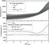 |
Fig. 1 Top: temperature structure of 3D, ⟨3D⟩, 1D LHD, and HM model atmosphere on the Rosseland optical depth scale. Bottom: horizontal temperature fluctuations, ΔTRMS, of the 3D model at constant τRoss (black) and temperature difference HM – ⟨3D⟩ (dashed) and 1D LHD – ⟨3D⟩ (blue) as a function of log τRoss. |
The temperature structure of the HM model is significantly different from that of the theoretical 1D LHD model atmospheres, as illustrated in Fig. 1. In the optical depth range −5.0 < log τRos< −0.5, the HM model is slightly warmer than the ⟨3D⟩ model by 50 to 100 K, while the 1D LHD model almost perfectly matches the ⟨3D⟩ model. In the deep photosphere (−0.5 < log τRos< + 0.5), where significant parts of the triplet lines originate, the HM model closely follows the temperature of the ⟨3D⟩ model, while the 1D LHD shows a somewhat steeper temperature gradient in these layers. This results in stronger OI triplet lines computed from the LHD model compared to those of the HM atmosphere.
3.2. 3D/1D non-LTE spectrum synthesis
Theoretical spectral lines were synthesized in two separate steps. Firstly, the departure coefficients6 of the atomic levels involved in the O i triplet were computed with the NLTE3D code. Then the departure coefficients were passed to the spectral line synthesis package Linfor3D that was used to compute spectral line profiles across the solar disk. In this section, we describe the basic assumptions and methods applied in the non-LTE spectrum synthesis calculations.
3.2.1. The oxygen model atom
We use an oxygen model atom that consists of 22 levels of O i (plus continuum), each having an associated bound-free transition. In addition, we take 64 bound-bound transitions into account, some of which are purely collisional. Figure 2 shows the Grotrian diagram of our model atom.
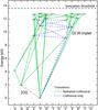 |
Fig. 2 Oxygen model atom used in this work. Radiatively allowed transitions are marked with green solid lines. Radiatively forbidden transitions, which were treated via electron-impact excitation only, are marked by blue dashed lines. The forbidden [O i] line and the O i IR triplet are marked by red dash-dotted lines. We took collisional and radiative bound-free transitions into account for each level. |
Level energies and statistical weights of the model atom were taken from the NIST Atomic Spectra Database Version 57 (see Table A.1). Cross sections for radiative, bound-free transitions were taken from the TOPBASE service8 of the Opacity Project (Cunto et al. 1993). Lacking reliable collisional cross sections derived from laboratory measurements or quantum-mechanical calculations, we resort to the classical prescriptions of Allen (Allen 1973, p. 41) and Drawin (Drawin 1969; Steenbock & Holweger 1984; Lambert 1993) to obtain the rate coefficients for bound-free transitions due to ionizing collisions with electrons and neutral hydrogen, respectively. As the Drawin approximation is highly uncertain (see Sect. 5.3 below), we scale the rates obtained from the Drawin formula by the adjustable parameter SH, which is deduced simultaneously with the oxygen abundance (see Sect. 4). Finally, we include the charge transfer reaction O0 + H+ ⇌ O+ + H0 for the ground level of oxygen, as described by Arnaud & Rothenflug (1985). Because the ionization potentials of O i and H i are similar, this reaction is nearly resonant and very efficient. It ensures that the ground level of O i is in equilibrium with O ii.
Out of the 64 bound-bound transitions, 54 are radiatively and collisionally permitted, while the remaining ten are radiatively forbidden. For the latter transitions, we only take collisions with electrons into account (see below). Einstein coefficients and wavelengths for the permitted transitions were again taken from the NIST Atomic Spectra Database (see Table A.2).
Rate coefficients for collisional excitation by neutral hydrogen were computed with classical Drawin formula and scaled by the same factor SH as applied to the ionizing collisions by neutral hydrogen. Since the collisional cross section according to the Drawin formalism is proportional to the oscillator strength gf of the transition, the levels of the radiatively forbidden transitions are also not coupled by hydrogen collisional excitation in our model atom. Alternative assumptions and their impact on the derived oxygen abundance are briefly discussed in Sect. 5.3.1 below.
Rate coefficients for the collisional excitation by e− were taken from the detailed R-matrix computations of Barklem (2007). For the radiatively allowed transitions that were not included in the latter work, we applied the classical van Regemorter’s formula (van Regemorter 1962). The rate coefficients of Barklem (2007), unlike those computed by the oscillator strength-dependent classical van Regemorter’s formula, are nonzero for radiatively forbidden transitions (blue dashed lines in Fig. 2), and hence we were able to account for the inter-system collisional transitions. The latter transitions are thought to play an important role in defining the statistical equilibrium of oxygen (especially at low metallicities, see Fabbian et al. 2009) and must be taken into account in realistic NLTE simulations. While the work of Barklem (2007) provides data for a total of 171 bound-bound transitions, we have only used 48 of them, based on the magnitude of their rate coefficient. We have performed tests that evaluate the influence of the remaining purely collisional transitions and found that it is negligible in the case of the Sun.
It should be noted that fine-structure splitting is ignored in our model atom, and all multiplets are treated as singlets. In particular, the upper level of the O i IR triplet, level 3p5P, is treated as a single superlevel with a single departure coefficient. However, since the three triplet components are well separated in wavelength, the line opacity computed from the combined gf-value of the superlevel transition would be too large, resulting in a wrong mean radiation field and, in turn, in wrong radiative excitation rates. To avoid this problem, we replace, for the radiative line transfer calculations only, the summed-up gf-value of the combined multiplet transition with the gf-value of the intermediate triplet component, thus diminishing the line opacity by a factor 3 (see Appendix B for additional information). Similar opacity scaling is applied for all other lines that involve multiplet transitions. This approach significantly reduces the computational cost of solving the statistical equilibrium equations.
3.2.2. Computation of departure coefficients with NLTE3D
As a first step towards computing 3D/1D non-LTE line profiles of the O i IR triplet, we computed departure coefficients bi, using the NLTE3D code with the 3D/1D solar model atmospheres and oxygen model atom described in the previous sections.
Firstly, NLTE3D computes the line-blanketed radiation field that is required for the calculation of the photoionization transition probabilities. For this task, we utilized the line opacity distribution functions from Castelli & Kurucz (2004) and the continuum opacities from the IONOPA package. The radiation field is derived with a long-characteristics method where the transfer equation is solved with a modified Feautrier scheme. To save computing time, continuum scattering is treated as true absorption. For solar conditions, the validity of the latter approximation has been verified via comparison with test calculations for a single 3D snapshot in which coherent isotropic continuum scattering is treated consistently. To further minimize the computational cost, we have reduced the spatial resolution of the 3D model by using only every third point in both horizontal directions, thus saving about 90% of the computing time. Tests have shown that this loss of spatial resolution does not influence the final results in any significant way (see Appendix C).
Based on this fixed 3D radiation field, we compute the photoionization and photorecombination transition probabilities. They are assumed to be independent of possible departures from LTE in the level population of O i. Then, NLTE3D computes the angle-averaged continuum intensities, Jcont, at the central wavelength of all of the line transitions. If a particular spectral line is weak, the profile averaged mean line intensity,  is fixed to Jcont, and the radiative bound-bound transition probabilities of these lines are only computed once. Finally, we compute the collisional transition probabilities, which only depend on the local temperature. All of those transition probabilities are fixed, as they do not depend on the departure coefficients. In this situation, the solution of the statistical equilibrium equations would be straightforward, and the departure coefficients of all levels could be obtained immediately, i.e., without any iterative procedure.
However, as soon as the line transitions are no longer optically thin, the mean radiative line intensities, , and the departure coefficients, bi, are inter-dependent quantities that exhibit a highly nonlinear coupling. In this case, we must compute as the weighted average of Jν over the local absorption profile, taking into account that line opacity and source function depend on the departure coefficients of the energy levels of the transition. In the present version of NLTE3D, the local line profile is assumed to be Gaussian, representing the thermal line broadening plus the effect of microturbulence. At this point, the 3D hydrodynamical velocity field is not used, so Doppler shifts along the line of sight are ignored. Instead, the velocity field is represented by a depth-independent microturbulence of 1.0 km s-1. Radiative damping, as well as van der Waals and Stark broadening, are ignored at this stage. We verified that this simplification has a negligible influence on the resulting departure coefficients. For the spectrum synthesis, however, the line broadening is treated in full detail and correctly includes the effects of the 3D hydrodynamical velocity field (see below).
Since it would be very computationally expensive to use complete linearization methods (Auer 1973; Kubát 2010, Sect. 8) with 3D model atmospheres, we choose to iterate between mean radiative line intensities and departure coefficients. However, as discussed by Prakapavičius et al. (2013), the solution of the oxygen non-LTE problem with NLTE3D by ordinary Λ-iteration exhibits a poor convergence, which could potentially lead to faulty results. Hence, we implemented the accelerated Λ-iteration (ALI) scheme of Rybicki & Hummer (1991, Sect. 2.2) to achieve faster convergence.
Iterations are started with LTE line opacities and source functions, from which the mean line intensities, , radiative transition probabilities, and equivalent widths (EWs) of the emergent flux line profiles are calculated. Then, all previously computed transition probabilities enter the equations of statistical equilibrium, which are solved for the unknown departure coefficients. Using the computed departure coefficients, the non-LTE line opacities and source functions are computed and the radiation transfer is solved for all relevant lines using these quantities. Then the , flux EWs, and approximate Λ-operators (Λ∗) are recomputed with non-LTE line opacities and source functions. The updated mean radiative intensities enter the equations of statistical equilibrium and the cycle begins again.
The accelerated Λ-iterations are continued until the relative changes (from one iteration to the next) in the flux EWs of all sufficiently strong lines have converged to less than 10-3. We checked that increasing the accuracy of the convergence criterion does not alter the resulting departure coefficients significantly, which might be ascribed to the good convergence properties of the accelerated Λ-iteration scheme.
In preparation for the following investigation, we computed departure coefficients for a grid of SH and A(O) values. The SH values range from 0 to 8/3 in steps of 1/3, and A(O) varies from 8.65 to 8.83 dex in steps of 0.03 dex. The spectrum synthesis calculations described in Sect. 3.2.3 are based on this rather extensive and dense grid of departure coefficients.
Since the NLTE3D code can only work with 3D model atmospheres defined on a geometrical grid, the 1D LHD and HM model atmospheres were converted to pseudo-3D models by replicating the particular 1D model atmosphere three times horizontally in each direction so that the resulting model would have 3 × 3 identical columns. Using the same equation of state and Rosseland opacity tables as in the 3D models, the vertical grid spacing of the pseudo-3D models is adjusted to ensure that the resulting model atmosphere is sampled at equidistant log τRoss levels, and preserves the T(τ) relation of the original 1D model.
3.2.3. 3D/1D NLTE spectrum synthesis with Linfor3D
The second step in computing the synthetic line profiles of the oxygen infrared triplet is the spectrum synthesis itself. Here we adopt the same atomic line parameters as specified in Table 1 of Paper I, and perform detailed 3D non-LTE line formation calculations with the Linfor3D9 package, which can handle both 3D and 1D model atmospheres. As in the case of the NLTE3D calculations of the departure coefficients, we reduced the horizontal resolution of the 3D model atmosphere by choosing only every third grid point in x and y-direction. Again, we conducted experiments confirming that this reduction does not influence the final results (see also Appendix C).
Linfor3D computes the LTE populations of the upper and lower levels involved in the triplet transitions via Saha-Boltzmann statistics using the IONOPA package10. From this, Linfor3D evaluates the LTE continuum and line opacities,  and
and  . Then it uses the previously derived departure coefficients to compute the NLTE line opacity
  and line source function
  (assuming complete redistribution), according to
 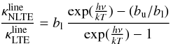 (1)and
 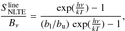 (2)where Bν is the Planck function, and bl and bu are the departure coefficients of the lower and upper level of the line transition, respectively (see, e.g., Mihalas 1978, Chap. 4–1). Note that both LTE and NLTE line opacities are corrected for stimulated emission. We recall that we assume all transitions of the oxygen 777 nm triplet to share identical departure coefficients bl and bu. The local line profiles are now represented by Voigt profiles, taking into account thermal broadening combined with van der Waals and natural line broadening11; differential Doppler shifts along the line of sight due to the 3D hydrodynamical velocity field are considered as well.
Using these ingredients, the radiative transfer equation is integrated on long characteristics to obtain the emergent radiative intensities as a function of wavelength. The intensity spectra are calculated for two sets of inclination angles μ, which represent the WCLC and Pereira et al. (2009b) observations (see Sect. 2 or Table 2), in each case for four azimuthal directions (0, π/ 2, π, 3/2 π). The final intensity spectrum for each μ is obtained by averaging over all surface elements, and to improve the statistics, over all azimuthal directions. For comparison with the solar flux spectrum, we computed the integral over μ of the μ-weighted intensity spectra using cubic splines to derive the disk-integrated flux profile.
We finally compute a grid of synthetic line profiles using the corresponding grid of departure coefficients described in the previous section. Each component of the oxygen triplet is synthesized for SH-values in the range from 0 to 8/3 (with steps of 1/3), and A(O)-values in the range between 8.65 and 8.83 (with steps of 0.03 dex).
4. Results
Computed synthetic intensity spectra are compared with observations across the solar disk to derive A(O) and SH simultaneously. For this task, we adopt two different methodologies in which we compare theoretical and observed line profiles and line equivalent widths, respectively. In this section, we describe the fitting procedures and their individual results.
4.1. Line profile fitting
Here we compare observed and theoretical intensity line profiles and search for the best-fitting A(O) – SH combination. This task utilizes the grid of theoretical NLTE line profiles described in Sect. 3.2.3) and searches for the A(O) – SH combination that provides the best fit of the intensity profiles of a single triplet component simultaneously at all μ-angles.
4.1.1. Fitting procedure
We employ the Levenberg-Markwardt least-squares fitting algorithm (Markwardt 2009), as implemented in IDL procedure MPFIT, to find the minimum χ2 in the four-dimensional parameter space defined by A(O), SH, vb, and Δλ. Here vb is the FWHM (in velocity space) of a Gaussian kernel, which is used to apply some extra line broadening to the synthetic spectra to account for instrumental broadening and, in the case of 1D model atmospheres, macroturbulence; Δλ is a global wavelength shift applied to the synthetic spectrum to compensate for potential imperfections of the wavelength calibration, uncertainties in the laboratory wavelengths, and systematic component- and μ-dependent line shifts. Test runs with an additional free fitting parameter for the continuum placement resulted in unsatisfactory fits. We therefore rely on the correct normalization of the observed spectra and consider the continuum level as fixed.
In a first sweep, we find the minimum χ2 for each triplet component k and each μ-angle individually. Here χ2 is defined as 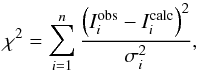 (3)where the sum is taken over all n considered wavelength points of the line profile,
  and
and  is the intensity of observed and synthetic normalized spectrum, respectively, and σi is the pixel-dependent observational uncertainty of the spectrum to be fitted. For simplicity, we have adopted a fixed continuum signal-to-noise ratio of S/N = 500 for both the WCLC and the Pereira spectra, and computed σi simply as σ = (S/N)-1, independent of wavelength point i and inclination angle μ.
An obvious blend in the blue wing of the strongest triplet component at λ 777.2 nm is excluded from the relevant wavelength range by masking a window between −374 and −214 mÅ from the line center, setting 1 /σi = 0 for these pixels.
The result of this χ2 minimization procedure is a set of best-fit parameters A(O), SH, vb, Δλ for each (k,μ). These intermediate results are only used for two purposes: (i) for fixing the relative wavelength shift of the line profiles as a function of μ for each triplet component k; and (ii) to “measure” the equivalent width of each individual observed line profile via numerical integration of the best-fitting synthetic line profile over a fixed wavelength interval of ±2 Å. The measured equivalent widths are used later for the equivalent width fitting method as described in Sect. 4.2.1.
We note that the oxygen abundance obtained from fitting the individual line profiles is relatively high, 8.78 <A(O) < 8.87, where the required oxygen abundance tends to increase towards the limb. At the same time, the corresponding SH-values are large as well (SH ≳ 3.0). However, we do not consider these results to be relevant because the line profile at a given single μ can be reproduced almost equally well with different combinations of the fitting parameters A(O), SH, and vb, which are tightly correlated. Small imperfections in the theoretical and/or observed line profiles can thus easily lead to ill-defined solutions. This degeneracy is only lifted when fitting the profiles at all μ-angles simultaneously.
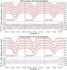 |
Fig. 3 Best-fitting non-LTE line profiles computed with the 3D model atmosphere for the WCLC (top) and Pereira (bottom) spectra. The top panels show the observed spectrum (black lines) and their theoretical best-fitting counterparts (red dots) for the different μ-angles, μ increasing from top (limb) to bottom (disk center). For clarity, a vertical offset of 0.1 was applied between consecutive μ-angles. The legend shows the best-fitting A(O) value for each of the three triplet lines. The bottom panels show the difference of the normalized intensites Iobs − Icalc. An offset of 0.01 was applied between the different μ-angles (μ increasing downwards). |
Results of non-LTE line profile fitting with various model atmospheres: A(O), SH-values, and reduced χ2 of the best fit for two different observed spectra (WCLC and Pereira 2009); the difference between A(O) derived from the two different spectra is given in Col. (4).
In the second sweep, we fit the line profiles at all μ-angles (μj,j = 1...m) simultaneously, but separately for each of the three triplet components. In this case, χ2 is defined as 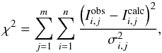 (4)where m is the number of considered μ-angles (μ ≳ 0.2). Again, σi,j is taken to be constant, σi,j = σ = (S/N)-1, as explained above, and the blend in the blue wing of the strongest triplet line at λ 777.2 nn is masked as before. Treating the triplet components separately has the advantage of allowing a consistency check and providing an independent error estimate of the derived oxygen abundance.
As in the first sweep, we consider A(O), SH, and vb as free fitting parameters, but instead of a single global Δλ, we introduce two global line shift parameters, Δλ1 and Δλ2, to allow for the most general case of a μ-dependent line shift correction, computed as Δλ(μ) = Δλ0(μ) + Δλ1 + Δλ2 (1 − μ), where Δλ0(μ) is the individual wavelength shift determined in the first sweep for the respective μ-angle. It turns out, however, that the results of the global fitting are insensitive to the detailed treatment of the line shifts.
4.1.2. Fitting results for the WCLC and Pereira spectra
Figure 3 shows the results of the simultaneous line profile fitting with the 3D-NLTE synthetic line profiles of the WCLC and Pereira spectrum, respectively. In general, the agreement between observation and model prediction is very good; the differences never exceed 1% of the continuum intensity and usually remain at a much lower level. Both the line wings and line core are represented very well at all inclination angles. The very satisfactory match we obtain between theory and observation suggests that both the velocity field and the thermal structure of our model atmosphere are realistic in the range of optical depths sampled by the O i IR triplet lines for inclination angles μ ≳ 0.2. In addition, the accurate reproduction of the observed line profiles suggests that our NLTE line formation technique is adequate, despite the possible shortcomings regarding the modeling of hydrogen collisions.
The corresponding fits obtained with the 1D hydrostatic models are collected in Appendix E. In general, the line profiles computed with the 1D hydrostatic model atmospheres result in a less satisfactory agreement with the observations. For example, given a single A(O) and SH value, the ⟨3D⟩ and 1D LHD models fail to simultaneously account for the line core and wings at μ = 1, and predict a much too weak line core close to the limb (see Figs. E.1 and E.3). The situation with the HM model (Fig. E.2) is better, but the line profile fits are still clearly inferior to those computed with the 3D model atmosphere. It is worth mentioning that, for all 1D model atmospheres, changing the (μ-independent) microturbulence parameter only changes the value of the best-fitting A(O) and SH, but does not improve the quality of the fits.
In Table 1, we summarize the main results derived from fitting the line profiles simultaneously for all μ-angles, separately for each of the three triplet components, and for both the WCLC and the Pereira observed spectra. Columns (2) and (3) list the best-fitting oxygen abundance A(O) and their formal fitting errors for WCLC and Pereira, respectively, and Col. (4) shows the difference between A(O) derived from the two different sets of spectra. Columns (5) and (6) give the corresponding results for SH, while the last two columns show the reduced χ2 of the best fit for the two sets of spectra, respectively, defined as  ), where p = 5 is the number of free fitting parameters. The fact that
  is of the order of unity means that the fit provided by the synthetic spectra is good (at least for the 3D model), given the assumed uncertainty of the observed spectral intensity of σi = 1 / 500. However, only relative χ2-values are considered meaningful for judging the quality of a fit.
The formal fitting errors of A(O) and SH given in Table 1 are computed as the square root of the corresponding diagonal elements of the covariance matrix of the fitting parameters, which is provided by the MPFIT procedure. The fact that these fitting errors are relatively small shows that the solution found by the fitting procedure is well defined. However, these formal errors do not account for possible systematic errors (e.g., due to imperfect continuum placement, unknown weak blends, insufficient time averaging, etc.), and hence the true errors are likely to be larger. In the case of the ⟨3D⟩ and LHD models, the formal errors are meaningless because the best fit would require SH< 0 (see below), and the constraint SH≥ 0 essentially enforces SH = 0.
As shown in Table 1, the oxygen abundances derived from the two sets of observed spectra generally agree within 0.03 dex or better, which is of the same order of magnitude as the line-to-line variation of A(O). The WCLC spectra produce systematically lower abundances. We attribute this to the systematically stronger lines at low μ compared to the Pereira et al. (2009b) data (cf. Fig. 4 below), which implies a reduced gradient W(μ), and, in turn, a lower SH and A(O), as explained in more detail in Sect. 5.2. In the case of the 3D model atmosphere, we consider the agreement in the derived A(O) between the different triplet lines and between the two sets of spectra as satisfactory.
In case of 1D LHD model atmospheres, the agreement between the best-fit parameters of the two spectra is nearly perfect, but this is again related to the fact that SH is forced to 0. The resulting fits are not good (high ), particularly at the lowest μ-angle, as mentioned above. The derived A(O) are significantly lower (by about −0.15 dex) than for the 3D case. Similar conclusions can be drawn for the ⟨3D⟩ model. The non-LTE oxygen abundance obtained with the 1D semi-empirical HM model atmosphere lies somewhere in between the 3D and the 1D LHD results. While SH is positive, the line profiles are poorly fitted, both at disk center and near the limb (see Fig. E.2), and the line-to-line variation of A(O) is rather high.
As will be discussed below in Sect. 5.2, all 1D results are systematically biased towards low SH and low A(O) values. In the following, we shall therefore ignore the 1D results for the determination of the solar oxygen abundance.
To estimate the solar oxygen abundance from the profile fitting method, we compute, separately for each of the two data sets, the average abundance, ⟨A(O)⟩, as the unweighted mean over the best-fitting A(O) values of the three triplet lines. These mean oxygen abundances are listed in Table 1 in the rows marked “Mean”, together with their errors, which in this case are defined by the standard deviation of the individual data points from the three triplet components.
From the 3D-NLTE synthetic spectra we find: ⟨A(O)⟩ = 8.747 ± 0.010 dex (WCLC spectra) and ⟨A(O)⟩ = 8.766 ± 0.006 dex (Pereira’s spectra). We note that the 1 σ error bars of the two results fail (by a narrow margin) to overlap, indicative of unaccounted systematic errors. We finally derive a two-spectra average of ⟨⟨A(O)⟩⟩ = 8.757 ± 0.01 dex (⟨⟨SH⟩⟩ = 1.6 ± 0.2).
4.1.3. Fitting of disk-center intensity and flux line profiles
As an independent consistency check, we also applied our line profile fitting procedure to the Neckel & Labs (1984) FTS spectra. In this case, we simultaneously fit the solar disk-center (Neckel Intensity) and disk-integrated (Neckel Flux) O i IR triplet line profiles. The blue wing of the 777.2 nm line is masked as before. The synthetic flux spectrum is computed by integration over μ of the μ-weighted intensity spectra available at the five inclinations defined by the Pereira spectra. Subsequently, the flux spectrum is broadened with the solar synodic projected rotational velocity vsini = 1.8 km s-1. The fitting parameters are again A(O), SH, instrumental broadening vb, and the individual line shifts Δλ1 and Δλ2 for intensity and flux profile, respectively.
Using the 3D non-LTE synthetic line profiles, we obtain an average oxygen abundance of A(O)= 8.80 ± 0.008, where this error refers to the formal fitting error; the line-to-line scatter is much smaller, ≲0.001 dex. The best-fitting mean SH value is 2.7 ± 0.25. As before, the quality of the fits is very satisfactory, with  , 0.84, and 1.13 for the three triplet components at λ 777.2, 777.4, and 777.5 nm, respectively.
Both A(O) and SH are significantly higher than inferred from the center-to-limb variation of the line profiles in the WCLC and Pereira spectra. We have to conclude that neither the formal fitting errors nor the line-to-line variation of A(O) represent a valid estimate of the true uncertainty of the derived oxygen abundance. Rather, systematic errors must be the dominating factor. We shall demonstrate in the next section that the result of simultaneously fitting the intensity and flux profiles is very sensitive to small errors in measuring or modeling the relative line strengths in the disk-center and integrated disk spectra. We therefore consider the oxygen abundance derived from fitting the spectra at several μ-angles simultaneously as more reliable.
4.2. Equivalent width fitting
Another possible methodology for estimating the solar oxygen abundance is based on the comparison of the observed equivalent widths (EWs) and their center-to-limb variation with their theoretical counterparts. Matching the EW of the lines is admittedly less precise than line profile fitting: it is possible that synthetic and observed EWs match perfectly, while the line profiles exhibit significantly different shapes. However, EW-fitting has the advantage of being simpler: there are only two free fitting parameters, A(O) and SH. The additional fitting parameters that were necessary in the case of line profile fitting, related to extra line broadening and line shifts, have no influence on the equivalent width and thus are irrelevant for the EW fitting procedure.
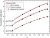 |
Fig. 4 Equivalent widths as measured in this work from WCLC and Pereira’s spectra (red and black lines, respectively), compared to the measurements taken from the work of Pereira et al. (2009b; black dots). See Table 2 for more details. |
4.2.1. Equivalent width measurements
For a given model atmosphere, a grid of theoretical equivalent widths, Wcalc(μ), is computed as a function A(O) and SH by integrating the non-LTE synthetic line profile over a wavelength interval of ±2 Å, separately for each triplet component. Here the inclination angle μ covers the values for both observed spectra (WCLC and Pereira). In addition, the equivalent widths of the disk-integrated line profiles were obtained by appropriate μ-integration, denoted as  in the following.
The EWs of the observed line profiles, Wobs(μ),  , are obtained as a by-product of the 3D non-LTE line profile fitting (see Sect. 4.1):
 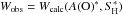 , where A(O)∗ and
  are the best-fit parameters for the respective line profile, obtained by fitting each μ-angle individually. This method of EW measurement ensures an optimal consistency between observed and theoretical equivalent widths. The errors of the observed EWs, σo, were estimated from the formal errors of A(O) and SH for the best-fitting theoretical line profile. The EWs of the O i IR triplet measured in this way are listed in Table 2 for all spectra; for the Pereira spectra, we also give the original measurements by Pereira et al. (2009b; bottom). The EWs from both the WCLC and the Pereira spectra, as collected in Table 2, are plotted in Fig. 4.
The EWs derived with our method from the Pereira spectra are generally slightly larger than those measured by the authors of the original work. This is because we integrate the synthetic single line profile over a very broad wavelength window. Since the O i lines have extended Lorentzian wings, our EWs are systematically higher. For the weakest lines at μ = 0.197, the impact of the Lorentzian wings is diminished, and the two measurements are in very close agreement (see Table 2). We argue that, for the purpose of EW fitting, our EW measurement method is superior to direct integration of the observed line profiles because it ensures consistency of theoretical and observed EWs.
4.2.2. EW fitting of disk-center and full-disk spectra
We first apply the method to determine SH and A(O) from the simultaneous fit of the disk-center and disk-integrated EWs in the Neckel intensity and flux spectra, respectively. For this purpose, we compute for each of the three triplet components two grids of equivalent widths, W(SH, A(O); μ = 1) and W(SH, A(O); flux), from the corresponding sets of 3D non-LTE line profiles. These grids are then used to construct contour lines in the SH – A(O) plane where Wcalc = Wobs, as shown in Fig. 5. The thick (red) solid line and the thick (green) dashed line refers to the EW measured in the Neckel disk-center and disk-integrated (flux) spectrum, respectively (see Table 2). The slope of the contour line of the flux EW is somewhat steeper than that for disk-center, indicating that the lines in the flux spectrum are slightly more sensitive to changes in SH. The unique solution (SH, A(O)) defined by the intersection point of the two lines (red diamond) is given in the legend of each panel.
EWs of the O i IR triplet as a function of μ measured from the different spectra with our line profile fitting method (this work).
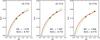 |
Fig. 5 Lines of constant equivalent width in the SH – A(O) plane, as computed from the grid of 3D non-LTE synthetic line profiles for the three triplet components. The thick (red) solid line refers to the EW measured in the Neckel disk-center spectrum, while the thick (green) dashed line is for the measured EW in the Neckel disk-integrated (flux) spectrum. The solution (SH, A(O)) given in the legend is defined by the intersection point of the two lines (red diamond). The black diamonds define the uncertainty range of the solution, assuming an EW measurement error of ≈0.5%, as indicated by the thin lines offset from the original SH – A(O) relations by ± ΔA(O) = 0.0025. |
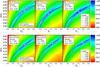 |
Fig. 6 Maps of χ2 (color-coded) in the SH – A(O) plane, indicating the quality of the simultaneous fit over all μ-angles of observed and computed 3D non-LTE EW, considering each of the three triplet components separately. The location of the minium χ2 is marked by a white plus sign, while the white ellipses bound the regions where |

Since the angle at which the two lines intersect is rather small, the position of the intersection point is very sensitive to the exact values of the two equivalent widths. To quantify the uncertainties, we have also plotted in Fig. 5 (thin lines) the contour lines shifted up and down by ΔA(O) = ± 0.0025 dex, corresponding to errors in EW of less than 0.5%. The black diamonds show the solutions obtained by changing the two EWs by this small amount in opposite directions. With this definition of the error bars, we find A(O) = 8.77 ± 0.02, SH = 1.85 ± 0.65.
These results are somewhat lower than the corresponding results obtained from line profile fitting (Sect. 4.1.3), with a marginal overlap of the error bars. We conclude that the idea of simultaneously fitting intensity and flux spectra works in principle, but is highly sensitive to small errors in the measured EWs and to systematic errors in modeling the μ dependence of the oxygen triplet lines. The results obtained with this method are therefore only considered a rough indication of the range of A(O) compatible with our modeling. As we see below, a more accurate determination of the oxygen abundance is possible when fitting simultaneously the line profiles measured at different μ-angles.
Results of non-LTE EW fitting with various model atmospheres: A(O), SH-values, and reduced χ2 of the best fit for two different observed spectra (WCLC and Pereira 2009); the difference between A(O) derived from the two different spectra is given in Col. (4).
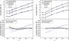 |
Fig. 7 Top panels: center-to-limb variation of observed (symbols) and theoretical EWs derived from the 3D model atmosphere for SH = 0 (blue dashed), 8/3 (red dotted) and best-fit value (black solid), shown individually for the three triplet components, with wavelength increasing from top to bottom. For each SH, the corresponding A(O) is defined as the value that minimizes χ2 (Eq. (5)) at fixed SH. Bottom panels: abundance difference |

4.2.3. EW fitting of the μ-dependent WCLC and Pereira spectra
We now determine SH and A(O) from the simultaneous fit of the EWs at all μ-angles, using the two independent sets of observed μ-dependent spectra of WCLC and Pereira, respectively. As before, we treat the three triplet components separately. In contrast to the method employed by Pereira et al. (2009b), we do not assign a special role to the fit at disk center. The idea of our method is to find the minimum χ2 in the SH – A(O) plane, where χ2 is defined as 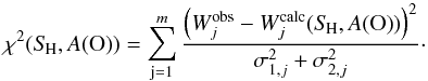 (5)We sum over the different μ-angles (j = 1...m); Wobs and Wcalc are the measured and computed equivalent width, respectively; σ1 is the measurement error of Wobs as given in Table 2, and σ2 is the observational error due to insufficient time averaging given the limited field of view covered by the slit on the solar surface. The error σ2 is only considered in case of the WCLC spectra, where the exposure times are less than the typical granule lifetime and the slit covers roughly three times the surface area of the 3D model. We derive σ2 from a bootstrap-like test, where a random subsample of three different snapshots is repeatedly drawn from a larger sample of 20 3D snapshots without replacement. For each μ-value, we generated 10 000 realizations of the possible appearance of the solar surface in the field of view, using the same A(O) – SH combination as for the equivalent width measurement (see above). The trial-to-trial variance of the derived distribution of the subsample averaged EWs is then taken as σ2. Pereira’s spectra have much better statistics (large number of observations per μ-angle), and there is no need to consider this kind of measurement error in the case of these spectra.
For the purpose of EW fitting, we compute a grid of equivalent widths, W(SH, A(O); μ) from the corresponding sets of 3D non-LTE line profiles, where 0 ≤ SH ≤ 8 / 3, 8.65 ≤ A(O) ≤ 8.83, and μ covering the observed limb angles. This allows us to compute χ2(SH,A(O)) in the SH – A(O) plane, separately for each of the three triplet components, as shown in Fig. 6 for both observational data sets. The best-fit solution is defined by the location of the minimum of χ2, as indicated in the plots by a white plus sign, which is found by EW interpolation using third-order polynomials.
The results of the EW fitting for various model atmospheres are summarized in Table 3, listing A(O) and SH of the best fit for the WCLC and Pereira observed spectra. The formal fitting errors of A(O) and SH are given by the projection of the contour line defined by  (white ellipse in Fig. 6) on the A(O) and SH axis, respectively. We also provide the reduced χ2 of the best fit, which is defined as
  ), where p = 2 is the number of free fitting parameters, as a measure of the quality of the fit.
The high quality of the EW fit achieved with the 3D model is also illustrated in Fig. 7, where we show the center-to-limb variation of observed and theoretical EWs for the best-fitting parameters and for the two extreme values SH = 0 and 8/3. Corresponding plots for all 1D model atmospheres investigated in this work are provided in Appendix F.
To derive the best estimate the solar oxygen abundance from EW fitting, we rely on the results of the 3D model atmosphere, which show the smallest line-to-line scatter and the lowest χ2. Computing the mean and errors for the two data sets as before in Sect. 4.1.2, we obtain ⟨A(O)⟩ = 8.754 ± 0.010 dex (WCLC data set) and ⟨A(O)⟩ = 8.771 ± 0.006 dex (Pereira data set). Again, the formal 1 σ error bars of these two abundance estimates do not overlap (by a narrow margin). Nevertheless, we derive the best estimate by averaging over the two data sets, arriving at ⟨⟨A(O)⟩⟩ = 8.763 ± 0.012, and ⟨⟨SH⟩⟩ = 1.6 ± 0.2. These numbers are fully consistent with the final result obtained from the line profile fitting described in Sect. 4.1.2. As in the latter case, the best-fit solutions, derived from the ⟨3D⟩ and 1D LHD modeling, turn out to be unphysical (negative SH). We discard these results as irrelevant and exclude them from Table 3 (see also Sect. 5.2 below).
5. Discussion
5.1. Comparison with the work of Pereira et al. (2009)
In the present work, we simultaneously derived the oxygen abundance, A(O), and the scaling factor for collisions with neutral hydrogen, SH, using two different methods of analyzing the μ-dependent spectra of the O i IR triplet: line profile fitting and equivalent width fitting. While the former method yields A(O) = 8.757 ± 0.010, SH = 1.6 ± 0.2, the latter gives A(O) = 8.763 ± 0.012, SH = 1.6 ± 0.2. In both methods, the spectra at the different μ-angles are assigned equal weight.
Pereira et al. (2009b) followed a different methodology, using a mix of EW fitting and line profile fitting, and assigning a distinguished role to the fits at disk center. More precisely, they first derive SH from simultaneously fitting the equivalent widths at all μ-angles and all three triplet components. For a given SH, the oxygen abundance is varied to find the local minimum χ2(SH). Then the minimum of this function defines the global minimum of χ2, which corresponds to their best-fitting global value of SH = 0.85. Fixing SH at this value, these authors determine the oxygen abundance by fitting the line profiles at disk center, separately for each triplet component, and average the resulting A(O) values to obtain their best estimate of the oxygen abundance, A(O) = 8.68.
In Fig. 8, we show a comparison of the A(O) – SH relation obtained from our 3D-NLTE modeling with the results of Pereira et al. (2009b), for each of the three triplet lines and the two different disk-center spectra. For a given SH, the oxygen abundance is determined from disk-center line profile fitting, as described in Sect. 4.1.1 (first sweep, but with fixed SH). The figure immediately shows that our A(O) – SH relation differs significantly from that of Pereira et al. (2009b, their Table 3), implying a systematically higher A(O) for given SH. For the value SH = 0.85, which was determined by Pereira et al. (2009b), our relation suggests A(O) ≈ 8.71−8.72. This value is clearly incompatible with the value A(O) ≈ 8.64−8.68, found by the latter authors. However, we are cautious about making a direct comparison of the A(O) – SH relations since possible differences in the particular implementation of the Drawin formula (definition of SH) might introduce a bias (see Sect. 5.3.1), except when SH = 0 and ∞ (LTE).
In addition, the line profile fits that we achieve with our 3D non-LTE synthetic line profiles (see Fig. 3) are superior to the fitting results shown in the work of Pereira et al. (2009b; see their Fig. 6 and Sect. 4.1.2.) where, generally, a less perfect agreement was found.
We can only speculate about what causes the systematic difference between our results and those obtained by Pereira et al. (2009b). Differences in the employed oxygen model atom, the adopted atomic data (like photoionization and collisional cross sections), and other numerical details entering the solution of the non-LTE rate equations, are among the prime suspects. Since we even see systematic A(O) differences of about 0.03 dex in LTE (right column of Fig. 8), we conclude that differences in the 3D hydrodynamical model atmospheres and/or the spectrum synthesis codes must also play a role.
It seems very likely that the above mentioned differences in the theoretical 3D plus non-LTE modeling are the main reason for the discrepancy in the final oxygen abundance of almost 0.1 dex between the present work and that of Pereira et al. (2009b). The different approaches of analyzing the data constitute an additional source of uncertainty.
5.1.1. Impact of equivalent width measurements
As described in Sect. 4.2.1, we systematically derive larger equivalent widths than Pereira et al. (2009b) near the disk center and lower EWs near the limb, from the same observed spectra (see Table 2) due to different measurement methods. One might therefore ask how much of the difference between the oxygen abundance derived in the present work and by Pereira et al. can be ascribed to differences in the measured equivalent widths. To answer this question, we have repeated our 3D, non-LTE, EW fitting procedure with the original equivalent widths as given by Pereira et al. (2009b). We find that the derived oxygen abundance decreases by ΔA(O) ≈ −0.045 dex, explaining roughly half the discussed A(O) discrepancy. We point out, however, that the almost perfect consistency between profile fitting and EW fitting results is destroyed if we were to adopt the equivalent widths measured by Pereira et al. (2009b). Note also that the mismatch illustrated in Fig. 8 is completely independent of any EW measurements.
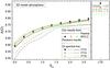 |
Fig. 8 Oxygen abundance determined from disk-center line profile fitting as a function of SH for the three triplet lines and the two different observed spectra. The 3D-NLTE results of the present work (solid lines, symbols) are compared with those of Pereira et al. (2009b, Table 3, dashed lines), obtained from their profile fits of the same disk-center spectra. |
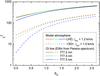 |
Fig. 9 Minimum χ2 as a function of SH obtained from global EW fitting with the ⟨3D⟩ and LHD model atmospheres. For each of the three triplet lines, we plot the minimum of χ2 (nonreduced) at fixed SH. No minimum of χ2 is found in the range 0 ≤ SH ≤ 8 / 3. At SH = 0, the implied oxygen abundances are A(O) = 8.61, 8.62, 8.63 (⟨3D⟩), and A(O) = 8.59, 8.60, 8.61 (LHD), for λ 777.2, 777.4, and 777.5 nm, respectively. The best fits would be obtained at negative SH and even lower A(O). |
5.2. Interpretation of the 1D results
As mentioned in Sect. 4.1, the oxygen abundance derived from line profile fitting based on 1D models (in particular ⟨3D⟩ and LHD) is significantly lower, by up to −0.15 dex, than the value derived with the 3D modeling. A very similar discrepancy between 1D and 3D results is obtained from the method of equivalent width fitting. The main reason is that the 1D models predict a steeper gradient of the line strength with respect to limb angle μ (compare Fig. 7 with Figs. F.1 and F.3). Under such circumstances, the best global fit of the observed center-to-limb variation of the triplet lines would formally require a negative SH, as demonstrated in Fig. 9. Because of the tight correlation between SH and A(O) (see Fig. 8), a low SH implies a low oxygen abundance: while SH ≈ 1.6 for the 3D model, SH ≡ 0 for the ⟨3D⟩ and LHD models, explaining the exceedingly low oxygen abundance derived with these 1D models. We add that our findings are in line with the results of Pereira et al. (2009b, their Fig. 5).
5.2.1. The microturbulence problem
Since the triplet lines are partially saturated, their formation is sensitive to the choice of the microturbulence parameter, ξmic, to be used with the 1D models. While the value of ξmic can be determined empirically, the main issue in the present context is the common assumption that ξmic is independent of μ. In fact, it is well known empirically that both micro- and macroturbulence increase towards the solar limb (e.g., Holweger et al. 1978). Evidently, we could improve the quality of the 1D fits by introducing a μ-dependent microturbulence parameter. With a more realistic ξmic increasing towards the limb, the slope of W(μ) at fixed A(O) would diminish, such that the best fit would require a larger (positive) SH and hence a higher oxygen abundance. Although it may be worthwhile, we have refrained from exploring the effects of a μ-dependent microturbulence on the results of the 1D models in the present work.
It is obvious that the 1D models with a fixed microturbulence are unrealistic, and lead to unphysical conclusions about the scaling factor (SH< 0). The oxygen abundance derived from these 1D models for the O i IR triplet lines is therefore systematically biased towards exceedingly low values. Even though the analysis based on the HM model atmosphere yields positive SH values, the resulting A(O) is considered as misleading, too, since the HM model suffers from the same microturbulence issues as the ⟨3D⟩ and LHD models, albeit in a less obvious way, because the problems are somehow masked by the empirical temperature structure of the HM model. Consequently, we have ignored all 1D results for the estimation of the final solar oxygen abundance. We rather rely on the analysis with the 3D model, which has a built-in hydrodynamical velocity field that properly represents a μ-dependent micro- and macroturbulence.
5.2.2. 1D–3D comparison
As described above, the microturbulence problem renders a direct comparison of the abundance determinations from 1D and 3D models meaningless. Nevertheless, it is possible to ask what oxygen abundance would be obtained from the 1D models if we use the same SH-value as found in the 3D analysis, i.e., considering this SH-value as a property of the model atom. Fixing SH in this way, we determined A(O) from the 1D models by fitting the observed equivalent width at disk center, assuming the canonical microturbulence value of ξmic = 1.0 km s-1. The results are summarized in Table 4.
Remarkably, the HM model atmosphere requires almost exactly the same oxygen abundance as the 3D model to match the measured disk-center equivalent width. This is indeed what is expected from a semi-empirical model. The averaged 3D model gives only a slightly lower A(O), suggesting that the effect of horizontal inhomogeneities is of minor importance, at least for the line formation at μ = 1. In contrast, the LHD model indicates a significantly lower oxygen abundance, which we attribute to the somewhat steeper temperature gradient in the line forming region (see Sect. 3.1.3).
5.3. Treatment of inelastic collisions by neutral hydrogen
Collisions of neutral oxygen atoms with neutral hydrogen give rise to bound-bound (excitation) and bound-free (ionization) transitions. As shown previously, they play a very important role in establishing the statistical equilibrium level population of O i. Unfortunately, quantum mechanical calculations or experimental measurements of the relevant collisional cross sections are so far unavailable. We have therefore resorted to calculating the excitation and ionization rates due to collisions by neutral hydrogen by the classical Drawin formula. Following common practice, we scaled the resulting rates by an adjustable factor, SH, which is determined from the best fit to the observations together with the oxygen abundance, as detailed above.
5.3.1. Alternative implementations of the Drawin formula
In the present work, the cross sections for inelastic collisions with neutral hydrogen are computed according to the classical recipe of Drawin (Drawin 1969; Steenbock & Holweger 1984; Lambert 1993), and hence are proportional to the oscillator strength f for all bound-bound transitions. For optically forbidden transitions, the collisional cross section is therefore zero. All hydrogen related collision rates included in our oxygen model atom, bound-bound and bound-free, are then scaled by the same factor SH. It is not clear whether other authors (e.g., Pereira et al. 2009b) might have adopted different assumptions. We have therefore investigated two test cases to understand the consequences for the derived oxygen abundance of (i) allowing for collisional coupling through optically forbidden transitions; and (ii) assuming a constant collision strength independent of f for all allowed transitions.
To reduce the computational cost, we have restricted the test calculations to EW fitting of the Pereira data set, using the HM 1D model atmosphere with ξmic = 1.2 km s-1. The results are summarized in Table 5. The oxygen abundance and SH-factor obtained with the standard setup are shown in Cols. (2) and (3) (“Case 0”, cf. Table 3).
In “Case 1”, we have included collisional excitation for all possible transitions according to the Drawin formula, where the cross sections of the optically allowed transitions are proportional to the oscillator strength f (as in “Case 0”). In this case, an effective minimum oscillator strength of f = 0.001 is adopted for all forbidden transitions, including the transitions between the triplet and quintuplet system, as suggested by Fabbian et al. (2009). Scaling by SH is restricted to the allowed transitions. The effect of the additional collisional coupling via the forbidden transitions on the oxygen abundance derived from EW fitting of the triplet lines is marginal: on average, A(O) is reduced by only 0.004 dex.
In “Case 2”, the treatment of the collisional coupling in the forbidden transitions is the same as in “Case 1”, but the cross sections of all optically allowed transitions are computed with f = 1. Again, scaling by SH is restricted to the allowed transitions. The effect of removing the proportionality between collision strength and oscillator strength for the allowed transitions on the derived oxygen abundance amounts to ≈−0.01 dex, while the numerical value of the required SH is reduced by roughly a factor 2 with respect to “Case 0”.
The effects shown in Table 5 are expected to be of similar magnitude in the full 3D analysis. We conclude from this experiment that the oxygen abundance derived from the non-LTE analysis of the O i IR triplet lines is not particularly sensitive to the details of the implementation of the Drawin formula, even if the numerical value of SH can differ significantly.
Resulting oxygen abundance A(O) and scaling factor SH derived from non-LTE EW fitting of the Pereira data set, using the HM model atmosphere with ξmic = 1.2 km s-1.
5.3.2. Assumption of a universal SH
Although this approach is commonly accepted, the assumption of a universal scaling factor is questionable. It could well be that each line is characterized by a slightly different value of SH, and/or that individual bound-bound and bound-free transitions require significantly different scaling factors. This would not be surprising, as it is well known that the classical treatment of collisions does not have a rigorous physical foundation. In fact, such nonuniform scaling has recently been demonstrated for Mg + H by Barklem et al. (2012). In principle, SH should depend on temperature (see Barklem et al. 2011) and, because the different triplet lines form at different atmospheric heights, SH could be expected to vary slightly from line to line. Our analysis allows for this possibility, since we treat each of the triplet components separately. However, we do not find any systematic trend in SH with wavelength, and consider the line-to-line variation of SH as random, reflecting the intrinsic uncertainties of our method. With this reasoning, a systematic variation of SH as a function of the limb angle also seems unlikely, and our analysis assumes a μ-independent SH. In summary, the treatment of the collisions by neutral hydrogen in terms of the empirical scaling factor SH appears unsatisfactory.
6. Conclusions
The present analysis of the O i IR triplet is based on two data sets of intensity spectra recorded at different μ-angles across the solar disk: a set of spectrograms taken by one of the authors (WCL) with the rapid scan double-pass spectrometer at the McMath-Pierce Solar Telescope, Kitt Peak, on 12 September 2006, and the set of high-quality spectra used by Pereira et al. (2009b), observed with the Swedish 1-m Solar Telescope on Roque de Los Muchachos, La Palma, in May 2007.
The photospheric oxygen abundance, A(O), and the scaling factor for collisional excitation/ionization by neutral hydrogen, SH, were determined simultaneously, using two different χ2 fitting methods of minimizing the difference between observed and synthetic spectra. In the first method, we simultaneously fit the line profiles at all μ-angles. Averaging the results of the three triplet components and the two different sets of observed spectra, we find an oxygen abundance of A(O) = 8.757 ± 0.010 (SH = 1.6 ± 0.2), where the error is defined by the standard deviation of the individual results. In the second method, we fit equivalent widths instead of line profiles, and obtain a perfectly consistent result, A(O) = 8.763 ± 0.012 (SH = 1.6 ± 0.2).
The above numbers were derived by employing 3D non-LTE synthetic spectra, consistently taking non-LTE line formation in a 3D hydrodynamical model of the solar atmosphere into account. When performing the same analysis with synthetic spectra computed from various 1D model atmospheres, we obtain much less perfect line profile fits, a larger line-to-line variation of A(O) and SH, and a significantly lower value of the best-fitting oxygen abundance. We argue that the 1D results are systematically biased towards low SH and A(O) values, mainly as a consequence of the assumption of a μ-independent microturbulence. Consequently, we have ignored all 1D results for the estimation of the final solar oxygen abundance in the present work. We rather rely on the analysis with the 3D model, which has a built-in hydrodynamical velocity field that properly represents a μ-dependent micro- and macroturbulence.
All individual results derived from the various observations of the O i IR triplet lines with different analysis methods, fall in the range 8.74 <A(O) < 8.78. We thus arrive at a final 3D non-LTE oxygen abundance of A(O) = 8.76 ± 0.02. This coincides with the value recommended in Paper I (see also Caffau et al. 2011) based on various atomic O i lines, but is significantly higher than suggested by the analysis of Pereira et al. (2009b), who find A(O) = 8.68. The reason for this discrepancy of almost 0.1 dex is unknown. Presumably, differences in the 3D hydrodynamical model atmospheres (CO5BOLD versus STAGGER), in the employed oxygen model atom, or in the adopted atomic data may offer an explanation.
Atomic energy levels of the oxygen model atom used in this work.
The present detailed investigation leads us to conclude that, from the CO5BOLD perspective, a solar photospheric oxygen abundance lower than A(O) = 8.70 now appears very unlikely. In view of the recent laboratory measurements of Bailey et al. (2015), indicating that the iron opacity near the solar radiation/convection zone boundary is significantly higher than assumed so far, the conflict between surface chemical abundances and helioseismic models might thus be less severe than previously thought.
Finally, we note that the treatment of the collisions by neutral hydrogen in terms of an empirical scaling factor SH is far from satisfactory. The assumption that the same SH is valid for all transitions is questionable and introduces an additional systematic uncertainty of unknown magnitude in the determination of the photospheric solar oxygen abundance from the O i IR triplet. Clearly, accurate theoretical or experimental collisional cross sections for neutral oxygen are badly needed.
Online material
Appendix E: Supplementary plots: line profile fitting results for 1D model atmospheres
In this appendix, we show the observed center-to limb variation of the line profiles of the O i IR triplet, separately for each component, in comparison with the best-fit theoretical non-LTE line profiles derived from various 1D model atmospheres. The best-fit values of the oxygen abundance, A(O), are given in the legend of each plot, as well as in Table 1 (together with the best-fit SH values). The best fit correspond to the global minimum of χ2 as defined by Eq. (4), i.e., simultaneously fitting the line profiles at all μ-angles. The quality of the fit can be judged from the reduced χ2 values provided in the Table, as well as from the plots of the intensity difference Iobs−Icalc displayed below the plot of the line profiles.
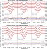 |
Fig. E.3 Same as in Fig. 3, except for the LHD model atmosphere with αMLT = 1.0 and ξmic = 1.2 km s-1. |
Appendix F: Supplementary plots: equivalent width fitting results
In this appendix, we show the center-to-limb variation of the observed equivalent widths, separately for each component of the O i IR triplet, in comparison with the theoretical results derived from various 1D model atmospheres. For given SH = 0 and 8/3, the oxygen abundance is computed as the A(O) value that minimizes the global χ2 given by Eq. (5). The best fit is defined as the
SH – A(O) combination that corresponds to the global minimum of χ2. The best-fit values of SH and A(O) are given in Table 3. The quality of the fit can be judged from the reduced χ2 values provided in the Table, as well as from the plots of the abundance difference  shown in the bottom panels of each Figure. Here A(μ) is the value of A(O) obtained from fitting the line profile separately at the individual μ-angle, while
  denotes the A(O) value derived from simultaneously fitting the line profiles at all μ-angles.
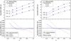 |
Fig. F.1 Same as in Fig. 7, except for the averaged 3D model atmosphere with ξmic = 1.0 km s-1. Best-fit solutions are not shown here, since they would require negative SH. |
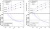 |
Fig. F.3 Same as in Fig. 7, except for the LHD model atmosphere with αMLT = 1.0 and ξmic = 1.2 km s-1. Best-fit solutions are not shown here, since they would require negative SH. |
[O / Fe] = log [ N(O)/N(Fe)]⋆−log [ N(O)/N(Fe)]⊙.
A(O) = log [ N(O)/N(H)] + 12.
μ = cosθ, where θ is the angle between the line of sight and the direction perpendicular to the solar surface; μ = 1 at disk center, while μ = 0 at the limb.
The only difference is that we now employ an equation of state that is consistent with the chemical abundance mix of the opacity tables.
The departure coefficient of atomic level i, bi, is defined as the ratio of non-LTE to LTE population number density,  .
.
Since this package is also utilized in NLTE3D, the calculations of departure coefficients and spectrum synthesis share consistent LTE number densities and continuum opacities.
Stark broadening is ignored here as in Paper I.
Acknowledgments
Part of this work was supported by grants from the Research Council of Lithuania (MIP-065/2013) and the French-Lithuanian programme “Gilibert” (TAP LZ 06/2013, Research Council of Lithuania). M.S. and H.G.L. acknowledge the funding of research visits to Vilnius by the Research Council of Lithuania. D.P. acknowledges financial support from the German Academic Exchange Service (DAAD) and AIP (Potsdam), which funded visits to Potsdam. E.C. is grateful to the FONDATION MERAC for funding her fellowship. H.G.L. acknowledges financial support by the Sonderforschungsbereich SFB881 “The Milky Way System” (subproject A4) of the German Research Foundation (DFG). The authors are also grateful to Sergii Korotin, Lyudmila Mashonkina, Tatyana Sitnova, and Paul Barklem for discussions regarding the non-LTE treatment of oxygen spectral lines. We thank the referee, Remo Collet, for his competent and constructive suggestions that helped us to further improve the presentation of our results.
References
- Allen, C. W. 1973, Astrophysical Quantities (Athlone Press) [Google Scholar]
- Allen de Prieto, C., Lambert, D. L., & Asplund, M. 2001, ApJ, 556, L63 [NASA ADS] [CrossRef] [Google Scholar]
- Allende Prieto, C., Asplund, M., & Fabiani Bendicho, P. 2004, A&A, 423, 1109 [NASA ADS] [CrossRef] [EDP Sciences] [Google Scholar]
- Arnaud, M., & Rothenflug, R. 1985, A&AS, 60, 425 [NASA ADS] [Google Scholar]
- Asplund, M., Grevesse, N., Sauval, A. J., Allen de Prieto, C., & Kiselman, D. 2004, A&A, 417, 751 [NASA ADS] [CrossRef] [EDP Sciences] [Google Scholar]
- Asplund, M., Grevesse, N., & Sauval, A. J. 2005, ASP Conf. Ser., 336, 25 [Google Scholar]
- Auer, L. 1973, ApJ, 180, 469 [NASA ADS] [CrossRef] [Google Scholar]
- Ayres, T. R., Lyons, J. R., Ludwig, H.-G., Caffau, E., & Wedemeyer-Böhm, S. 2013, ApJ, 765, 46 [NASA ADS] [CrossRef] [Google Scholar]
- Bailey, J. E., Nagayama, T., Loisel, G. P., et al. 2015, Nature, 517, 56 [NASA ADS] [CrossRef] [Google Scholar]
- Barklem, P. S. 2007, A&A, 462, 781 [NASA ADS] [CrossRef] [EDP Sciences] [Google Scholar]
- Barklem, P. S., Belyaev, A. K., Guitou, M., et al. 2011, A&A, 530, A94 [NASA ADS] [CrossRef] [EDP Sciences] [Google Scholar]
- Barklem, P. S., Belyaev, A. K., Spielfiedel, A., Guitou, M., & Feautrier, N. 2012, A&A, 541, A80 [NASA ADS] [CrossRef] [EDP Sciences] [Google Scholar]
- Basu, S., & Antia, H. M. 2008, Phys. Rep., 457, 217 [NASA ADS] [CrossRef] [Google Scholar]
- Beeck, B., Collet, R., Steffen, M., et al. 2012, A&A, 539, A121 [NASA ADS] [CrossRef] [EDP Sciences] [Google Scholar]
- Böhm-Vitense, E. 1958, Z. Astrophys., 46, 108 [Google Scholar]
- Caffau, E., 2009, Ph.D. Thesis, Observatoire de Paris [Google Scholar]
- Caffau, E., Ludwig, H.-G., Steffen, M., et al. 2008, A&A, 488, 1031 (Paper I) [CrossRef] [EDP Sciences] [Google Scholar]
- Caffau, E., Ludwig, H.-G., Steffen, M., Freytag, B., & Bonifacio, P. 2011, Sol. Phys., 268, 255 [NASA ADS] [CrossRef] [Google Scholar]
- Caffau, E., Ludwig, H.-G., Steffen, M., et al. 2015, A&A, 579, A88 [NASA ADS] [CrossRef] [EDP Sciences] [Google Scholar]
- Castelli, F., & Kurucz, R. L. 2004, ArXiv eprints [arXiv:astro-ph/0405087] [Google Scholar]
- Cunto, W., Mendoza, C., Ochsenbein, F., & Zeippen, C. J. 1993, A&A, 275, L5 [NASA ADS] [Google Scholar]
- Drawin, H. W. 1969, Z. Astrophys., 225, 483 [Google Scholar]
- Fabbian, D., Asplund, M., Barklem, P. S., Carlsson, M., & Kiselman, D. 2009, A&A, 500, 1221 [NASA ADS] [CrossRef] [EDP Sciences] [Google Scholar]
- Freytag, B., Steffen, M., Ludwig, H.-G., et al. 2012, J. Comp. Phys., 231, 919 [Google Scholar]
- Gratton, R. G., Carretta, E., Matteucci, F., & Sneden, C. 2000, A&A, 358, 671 [NASA ADS] [Google Scholar]
- Grevesse, N., & Sauval, A. J. 1998, Space Sci. Rev., 85, 161 [NASA ADS] [CrossRef] [Google Scholar]
- Gustafsson, B., Edvardsson, B., Eriksson, K., Jørgensen, U. G., Nordlund, Å., et al. 2008, A&A, 486, 951 [NASA ADS] [CrossRef] [EDP Sciences] [Google Scholar]
- Holweger, H. 1967, Z. Astrophys., 65, 365 [Google Scholar]
- Holweger, H., & Mueller, E. A. 1974, Sol. Phys., 39, 19 [NASA ADS] [CrossRef] [Google Scholar]
- Holweger, H., Gehlsen, M., & Ruland, F. 1978, A&A, 70, 537 [NASA ADS] [Google Scholar]
- Kiselman, D. 1991, A&A, 245, L9 [NASA ADS] [Google Scholar]
- Kiselman, D. 1993, A&A, 275, 269 [Google Scholar]
- Kubát, J. 2010, EAS Pub. Ser., 43, 1 [Google Scholar]
- Lambert, D. L. 1993, Phys. Scr. Vol. T, 47, 186 [NASA ADS] [CrossRef] [Google Scholar]
- Livingston, W., Wallace, L., White, O. R., & Giampapa, M. S. 2007, ApJ, 657, 1137 [NASA ADS] [CrossRef] [Google Scholar]
- Ludwig, H.-G., Jordan, S., & Steffen, M. 1994, A&A, 284, 105 [NASA ADS] [Google Scholar]
- Ludwig, H.-G., Caffau, E., Steffen, M., et al. 2009, Mem. Soc. Astron. It., 80, 711 [NASA ADS] [Google Scholar]
- Markwardt, C. B. 2009, Astronomical Data Analysis Software and Systems XVIII, 411, 251 [NASA ADS] [Google Scholar]
- Matteucci, F., & François, P. 1992, A&A, 262, L1 [NASA ADS] [Google Scholar]
- Mihalas, D. 1978, Stellar Atmospheres, Freeman and Company (San Fransisco: W. H. Freeman and Co.) [Google Scholar]
- Neckel, H. 1999, Sol. Phys., 184, 421 [NASA ADS] [CrossRef] [Google Scholar]
- Neckel, H., & Labs, D. 1984, Sol. Phys., 90, 205 [NASA ADS] [CrossRef] [Google Scholar]
- Nordlund, Å. 1982, A&A, 107, 1 [Google Scholar]
- Pereira, T. M. D., Kiselman, D., & Asplund, M. 2009a, A&A, 507, 417 [NASA ADS] [CrossRef] [EDP Sciences] [Google Scholar]
- Pereira, T. M. D., Asplund, M., & Kiselman, D. 2009b, A&A, 508, 1403 [NASA ADS] [CrossRef] [EDP Sciences] [Google Scholar]
- Prakapavičius, D., Steffen, M., Kučinskas, A., et al. 2013, Mem. Soc. Astron. It. Supp., 24, 111 [Google Scholar]
- Przybilla, N., Butler, K., Becker, S. R., Kudritzki, R. P., & Venn, K. A. 2000, A&A, 359, 1085 [NASA ADS] [Google Scholar]
- Rybicki, G. B., & Hummer, D. G. 1991, A&A, 245, 171 [NASA ADS] [Google Scholar]
- Scharmer, G. B., Bjelksjo, K., Korhonen, T. K., Lindberg, B., & Petterson, B. 2003, Proc. SPIE, 4853, 341 [Google Scholar]
- Steenbock, W., & Holweger, H. 1984, A&A, 130, 319 [NASA ADS] [Google Scholar]
- van Regemorter, H. 1962, ApJ, 136, 906 [NASA ADS] [CrossRef] [Google Scholar]
- Villante, F. L., Serenelli, A. M., Delahaye, F., & Pinsonneault, M. H. 2014, ApJ, 787, 13 [NASA ADS] [CrossRef] [Google Scholar]
- Vögler, A., Bruls, J. H. M. J., & Schüssler, M. 2004, A&A, 421, 741 [NASA ADS] [CrossRef] [EDP Sciences] [Google Scholar]
Appendix A: The oxygen model atom designed for solar applications
In Tables A.1 and A.2, we provide details about the 22 energy levels and 54 radiative transitions considered in the oxygen model atom used in this work. The data are taken from the NIST Atomic Spectra Database12.
Radiative transitions included in the oxygen model atom used in this work.
Appendix B: Ignoring the fine-structure splitting of the triplet
In Sect. 3.2.1, we mentioned that the upper level of the O i IR triplet (3p5P) is treated as a single superlevel in our oxygen model atom, thus ignoring the fine structure splitting of this term. Since the energy differences between fine-structure levels are negligible, the LTE population of this superlevel equals the sum of those of the individual sublevels. If the fine-structure levels are merged into one superlevel, the three transitions making up the triplet are merged into a single combined transition, and the gf-value of this combined transition is the sum of the gf-values of the individual fine-structure components.
The radiative transition probability (Einstein coefficient or, equivalently, gf-value) of a bound-bound transition plays a two-fold role in the non-LTE problem: firstly, the photoexcitation rate at given radiation field scales with gf; and secondly, the line opacity is proportional to gf, and hence the radiation field of the transition is a (nonlinear) function of the gf-value. Since the three triplet components are well separated in wavelength and partially saturated in the Sun, merging them leads to a strongly saturated single line where the mean radiation field in the line, , is diminished below the value in any of the individual original triplet components. The photoexcitation rates in the combined transition would therefore be significantly underestimated.
To avoid this systematic bias, we reduce the line opacity of the combined triplet transition by a factor 3. This is equivalent to using, only for the calculation of , the gf-value of the intermediate triplet component instead of the sum of the gf-values of all components. For the calculation of the photoexcitation rates at given radiation field, however, the total gf-value (i.e., the sum of the gf-values of the individual fine structure components) is applied. This procedure guarantees both and photoexcitation rates to be consistent with the real situation.
In the following, we show that the adopted approach is equivalent to having a detailed multiplet transition with three lines, with highly efficient collisions between the fine-structure levels. The latter approach was utilized in numerous works (e.g., Kiselman 1993; Przybilla et al. 2000; Asplund et al. 2004) and is assumed to be a valid representation of the real situation. To demonstrate the equivalence of the two methods, we constructed a model atom that includes the fine-structure splitting of the 3p5P level. We used a solar LHD model atmosphere to compute the departure coefficients for three cases:
-
1.
using the standard model atom where 3p5P is treated as a superlevel and gf is reduced by 1/3 for the calculation of the line opacity;
-
2.
using a model atom that includes the splitting of the 3p5P term and no collisional coupling between the fine-structure levels;
-
3.
using a model atom that includes the splitting of the 3p5P term and strong collisional coupling between the fine-structure levels.
In the last two cases, no scaling of the line opacity is applied. Except for the treatment of the 3p5P term and the transitions that connect to it, all three model atoms are identical (see Sect. 3.2.1). For the test calculations, the oxygen abundance was set to A(O) = 8.77 and SH = 1.0.
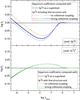 |
Fig. B.1 Departure coefficients of the O i IR triplet levels as a function of the optical depth for three cases of the fine-structure treatment (see text for details). The black solid line shows the results obtained when 3p5P is treated as a superlevel (case 1); colored lines show the results when fine-structure splitting is included; dashed lines show case 2 (no collisional coupling between fine-structure levels); solid lines show case 3 (strong collisional coupling between fine-structure levels). Top and bottom panels refer to terms 3p5P (upper level of the triplet) and 3s5So (lower level of the triplet), respectively. |
The results of this experiment are shown in Fig. B.1. Firstly, it is clear that the treatment of the level 3p5P does not significantly influence the lower level population of the triplet. This means that non-LTE line opacity of the O i IR triplet is not sensitive to the details regarding the fine-structure of 3p5P. Secondly, it is evident that, when no collisional coupling is applied between fine-structure levels, they exhibit slightly different departure coefficients. Our analysis (not detailed here) has shown that this is caused by the different line strengths of the three triplet components, which leads to different photoexcitation rates in each of the triplet transitions and, in turn, to different departure coefficients. Finally, the most important result is that, when efficient collisions between the fine-structure levels are applied, the departure coefficients of the individual sublevels thermalize to the same value that was computed with the superlevel approach. We consider this as a validation of our simplified approach, which reduces the number of lines for which the radiation transfer has to be computed and thus facilitates a faster solution (by about 60%) of the non-LTE statistical equilibrium problem.
Appendix C: Effect of horizontal resolution on the 3D-NLTE synthetic spectrum
In Sects. 3.2.2 and 3.2.3, we have mentioned that to speed up the calculations, we applied a horizontal reduction of the model atmosphere, using only every third vertical column in each horizontal direction (i.e., discarding 90% of the data defining the 3D model atmosphere). In this section, we briefly validate this approach.
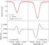 |
Fig. C.1 Effect of reduced horizontal resolution on the 3D-NLTE spectral line profile of the middle component of the O i IR triplet. Top panels: synthetic spectral lines computed with full resolution (black line) and with resolution reduced by a factor 3 in each horizontal direction (red dots). Bottom panels: difference in residual intensity between synthetic spectral lines computed with full and reduced horizontal resolution. A negative difference means that the spectral line computed with full resolution is stronger at the particular wavelength. Left and right panels show the results at μ = 0.2 and μ = 1.0, respectively. |
To estimate the effect of the reduced horizontal resolution, we performed non-LTE calculations (Sect. 3.2.2) and subsequent spectrum synthesis (Sect. 3.2.3) with a fully resolved single 3D model snapshot. In these calculations, we set A(O) = 8.77 and SH = 1.0. To see how the effect changes across the solar disk, spectrum synthesis was performed at two inclination angles: μ = 1.0 and μ = 0.2.
Figure C.1 shows the results of this experiment. It is seen that the effect of the reduced horizontal resolution does not exceed 0.1% of the continuum intensity anywhere in the line profile. The effect on equivalent widths is even smaller, δW/W ≈ 7 × 10⁻⁴ and 12 × 10-4 for μ = 0.2 and μ = 1.0, respectively. Hence we may conclude that the reduced horizontal resolution that we have imposed on the spectrum synthesis does not influence the results in any significant way.
Appendix D: Influence of the mixing-length parameter on 1D-NLTE spectrum synthesis of the O i IR triplet lines
The O i IR triplet lines share a lower level of high excitation potential and, hence, are expected to form in the deep photosphere. It could therefore be expected that 1D-NLTE spectral line synthesis of such lines is influenced by the choice of the mixing-length parameter, αMLT, which quantifies the convective efficiency and thus controls the temperature structure of the lower photosphere. To probe the possible influence of αMLT, we computed a grid of 1D-NLTE line profiles using solar LHD model atmospheres computed with the different values of αMLT. This grid of synthetic spectra is used to perform the same line profile fitting as described in Sect. 4.1.
Despite the fact that the fits are quite bad in general (see discussion in Sect. 4.1 and Fig. E.3), we arrived at very similar results regardless of the chosen αMLT. Table D.1 shows the results of line profile fitting with different values of αMLT and fixed ξmic = 1.2 km s-1 (assuming ξmic = 0.8 km s-1 yields similar conclusions). Varying αMLT between 0.5 and 1.5 changes the best-fitting A(O) by at most 0.006 dex (for the weakest triplet component). Also, the reduced χ2 values of the best fit are only marginally influenced. We conclude that A(O) is very weakly dependent on the choice of αMLT, and the goodness of the fits cannot be improved by modifying αMLT. Hence our results derived from LHD models with αMLT = 1.0 should be representative for all theoretical 1D mixing-length models of the solar atmosphere.
Best-fitting A(O) derived from the two sets of observed spectra, using 1D LHD model atmospheres with different αMLT values between 0.5 and 1.5, and fixed ξmic = 1.2 km s-1.
All Tables
Results of non-LTE line profile fitting with various model atmospheres: A(O), SH-values, and reduced χ2 of the best fit for two different observed spectra (WCLC and Pereira 2009); the difference between A(O) derived from the two different spectra is given in Col. (4).
EWs of the O i IR triplet as a function of μ measured from the different spectra with our line profile fitting method (this work).
Results of non-LTE EW fitting with various model atmospheres: A(O), SH-values, and reduced χ2 of the best fit for two different observed spectra (WCLC and Pereira 2009); the difference between A(O) derived from the two different spectra is given in Col. (4).
Resulting oxygen abundance A(O) and scaling factor SH derived from non-LTE EW fitting of the Pereira data set, using the HM model atmosphere with ξmic = 1.2 km s-1.
Best-fitting A(O) derived from the two sets of observed spectra, using 1D LHD model atmospheres with different αMLT values between 0.5 and 1.5, and fixed ξmic = 1.2 km s-1.
All Figures
|
Fig. 1 Top: temperature structure of 3D, ⟨3D⟩, 1D LHD, and HM model atmosphere on the Rosseland optical depth scale. Bottom: horizontal temperature fluctuations, ΔTRMS, of the 3D model at constant τRoss (black) and temperature difference HM – ⟨3D⟩ (dashed) and 1D LHD – ⟨3D⟩ (blue) as a function of log τRoss. |
| In the text | |
|
Fig. 2 Oxygen model atom used in this work. Radiatively allowed transitions are marked with green solid lines. Radiatively forbidden transitions, which were treated via electron-impact excitation only, are marked by blue dashed lines. The forbidden [O i] line and the O i IR triplet are marked by red dash-dotted lines. We took collisional and radiative bound-free transitions into account for each level. |
| In the text | |
|
Fig. 3 Best-fitting non-LTE line profiles computed with the 3D model atmosphere for the WCLC (top) and Pereira (bottom) spectra. The top panels show the observed spectrum (black lines) and their theoretical best-fitting counterparts (red dots) for the different μ-angles, μ increasing from top (limb) to bottom (disk center). For clarity, a vertical offset of 0.1 was applied between consecutive μ-angles. The legend shows the best-fitting A(O) value for each of the three triplet lines. The bottom panels show the difference of the normalized intensites Iobs − Icalc. An offset of 0.01 was applied between the different μ-angles (μ increasing downwards). |
| In the text | |
|
Fig. 4 Equivalent widths as measured in this work from WCLC and Pereira’s spectra (red and black lines, respectively), compared to the measurements taken from the work of Pereira et al. (2009b; black dots). See Table 2 for more details. |
| In the text | |
|
Fig. 5 Lines of constant equivalent width in the SH – A(O) plane, as computed from the grid of 3D non-LTE synthetic line profiles for the three triplet components. The thick (red) solid line refers to the EW measured in the Neckel disk-center spectrum, while the thick (green) dashed line is for the measured EW in the Neckel disk-integrated (flux) spectrum. The solution (SH, A(O)) given in the legend is defined by the intersection point of the two lines (red diamond). The black diamonds define the uncertainty range of the solution, assuming an EW measurement error of ≈0.5%, as indicated by the thin lines offset from the original SH – A(O) relations by ± ΔA(O) = 0.0025. |
| In the text | |
|
Fig. 6 Maps of χ2 (color-coded) in the SH – A(O) plane, indicating the quality of the simultaneous fit over all μ-angles of observed and computed 3D non-LTE EW, considering each of the three triplet components separately. The location of the minium χ2 is marked by a white plus sign, while the white ellipses bound the regions where |
| In the text | |
|
Fig. 7 Top panels: center-to-limb variation of observed (symbols) and theoretical EWs derived from the 3D model atmosphere for SH = 0 (blue dashed), 8/3 (red dotted) and best-fit value (black solid), shown individually for the three triplet components, with wavelength increasing from top to bottom. For each SH, the corresponding A(O) is defined as the value that minimizes χ2 (Eq. (5)) at fixed SH. Bottom panels: abundance difference |
| In the text | |
|
Fig. 8 Oxygen abundance determined from disk-center line profile fitting as a function of SH for the three triplet lines and the two different observed spectra. The 3D-NLTE results of the present work (solid lines, symbols) are compared with those of Pereira et al. (2009b, Table 3, dashed lines), obtained from their profile fits of the same disk-center spectra. |
| In the text | |
|
Fig. 9 Minimum χ2 as a function of SH obtained from global EW fitting with the ⟨3D⟩ and LHD model atmospheres. For each of the three triplet lines, we plot the minimum of χ2 (nonreduced) at fixed SH. No minimum of χ2 is found in the range 0 ≤ SH ≤ 8 / 3. At SH = 0, the implied oxygen abundances are A(O) = 8.61, 8.62, 8.63 (⟨3D⟩), and A(O) = 8.59, 8.60, 8.61 (LHD), for λ 777.2, 777.4, and 777.5 nm, respectively. The best fits would be obtained at negative SH and even lower A(O). |
| In the text | |
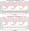 |
Fig. E.1 Same as in Fig. 3, except for the averaged 3D model atmosphere with ξmic = 1.0 km s-1. |
| In the text | |
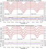 |
Fig. E.2 Same as in Fig. 3, except for the Holweger-Müller model atmosphere with ξmic = 1.2 km s-1. |
| In the text | |
|
Fig. E.3 Same as in Fig. 3, except for the LHD model atmosphere with αMLT = 1.0 and ξmic = 1.2 km s-1. |
| In the text | |
|
Fig. F.1 Same as in Fig. 7, except for the averaged 3D model atmosphere with ξmic = 1.0 km s-1. Best-fit solutions are not shown here, since they would require negative SH. |
| In the text | |
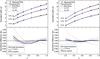 |
Fig. F.2 Same as in Fig. 7, except for the Holweger-Müller model atmosphere with ξmic = 1.2 km s-1. |
| In the text | |
|
Fig. F.3 Same as in Fig. 7, except for the LHD model atmosphere with αMLT = 1.0 and ξmic = 1.2 km s-1. Best-fit solutions are not shown here, since they would require negative SH. |
| In the text | |
|
Fig. B.1 Departure coefficients of the O i IR triplet levels as a function of the optical depth for three cases of the fine-structure treatment (see text for details). The black solid line shows the results obtained when 3p5P is treated as a superlevel (case 1); colored lines show the results when fine-structure splitting is included; dashed lines show case 2 (no collisional coupling between fine-structure levels); solid lines show case 3 (strong collisional coupling between fine-structure levels). Top and bottom panels refer to terms 3p5P (upper level of the triplet) and 3s5So (lower level of the triplet), respectively. |
| In the text | |
|
Fig. C.1 Effect of reduced horizontal resolution on the 3D-NLTE spectral line profile of the middle component of the O i IR triplet. Top panels: synthetic spectral lines computed with full resolution (black line) and with resolution reduced by a factor 3 in each horizontal direction (red dots). Bottom panels: difference in residual intensity between synthetic spectral lines computed with full and reduced horizontal resolution. A negative difference means that the spectral line computed with full resolution is stronger at the particular wavelength. Left and right panels show the results at μ = 0.2 and μ = 1.0, respectively. |
| In the text | |
Current usage metrics show cumulative count of Article Views (full-text article views including HTML views, PDF and ePub downloads, according to the available data) and Abstracts Views on Vision4Press platform.
Data correspond to usage on the plateform after 2015. The current usage metrics is available 48-96 hours after online publication and is updated daily on week days.
Initial download of the metrics may take a while.