| Issue |
A&A
Volume 583, November 2015
|
|
|---|---|---|
| Article Number | A57 | |
| Number of page(s) | 23 | |
| Section | The Sun | |
| DOI | https://doi.org/10.1051/0004-6361/201526406 | |
| Published online | 27 October 2015 | |
Online material
Appendix E: Supplementary plots: line profile fitting results for 1D model atmospheres
In this appendix, we show the observed center-to limb variation of the line profiles of the O i IR triplet, separately for each component, in comparison with the best-fit theoretical non-LTE line profiles derived from various 1D model atmospheres. The best-fit values of the oxygen abundance, A(O), are given in the legend of each plot, as well as in Table 1 (together with the best-fit SH values). The best fit correspond to the global minimum of χ2 as defined by Eq. (4), i.e., simultaneously fitting the line profiles at all μ-angles. The quality of the fit can be judged from the reduced χ2 values provided in the Table, as well as from the plots of the intensity difference Iobs−Icalc displayed below the plot of the line profiles.
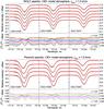 |
Fig. E.1
Same as in Fig. 3, except for the averaged 3D model atmosphere with ξmic = 1.0 km s-1. |
| Open with DEXTER | |
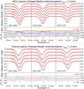 |
Fig. E.2
Same as in Fig. 3, except for the Holweger-Müller model atmosphere with ξmic = 1.2 km s-1. |
| Open with DEXTER | |
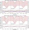 |
Fig. E.3
Same as in Fig. 3, except for the LHD model atmosphere with αMLT = 1.0 and ξmic = 1.2 km s-1. |
| Open with DEXTER | |
Appendix F: Supplementary plots: equivalent width fitting results
In this appendix, we show the center-to-limb variation of the observed equivalent widths, separately for each component of the O i IR triplet, in comparison with the theoretical results derived from various 1D model atmospheres. For given SH = 0 and 8/3, the oxygen abundance is computed as the A(O) value that minimizes the global χ2 given by Eq. (5). The best fit is defined as the
SH – A(O) combination that corresponds to the global minimum of χ2. The best-fit values of SH and A(O) are given in Table 3. The quality of the fit can be judged from the reduced χ2 values provided in the Table, as well as from the plots of the abundance difference ![]() shown in the bottom panels of each Figure. Here A(μ) is the value of A(O) obtained from fitting the line profile separately at the individual μ-angle, while
shown in the bottom panels of each Figure. Here A(μ) is the value of A(O) obtained from fitting the line profile separately at the individual μ-angle, while ![]() denotes the A(O) value derived from simultaneously fitting the line profiles at all μ-angles.
denotes the A(O) value derived from simultaneously fitting the line profiles at all μ-angles.
 |
Fig. F.1
Same as in Fig. 7, except for the averaged 3D model atmosphere with ξmic = 1.0 km s-1. Best-fit solutions are not shown here, since they would require negative SH. |
| Open with DEXTER | |
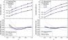 |
Fig. F.2
Same as in Fig. 7, except for the Holweger-Müller model atmosphere with ξmic = 1.2 km s-1. |
| Open with DEXTER | |
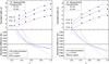 |
Fig. F.3
Same as in Fig. 7, except for the LHD model atmosphere with αMLT = 1.0 and ξmic = 1.2 km s-1. Best-fit solutions are not shown here, since they would require negative SH. |
| Open with DEXTER | |
© ESO, 2015
Current usage metrics show cumulative count of Article Views (full-text article views including HTML views, PDF and ePub downloads, according to the available data) and Abstracts Views on Vision4Press platform.
Data correspond to usage on the plateform after 2015. The current usage metrics is available 48-96 hours after online publication and is updated daily on week days.
Initial download of the metrics may take a while.