© ESO, 2015

1. Introduction

The central black holes in quasars accrete the matter in their surroundings and emit light over the whole electromagnetic range. The standard model of continuum emission from an accretion disc devised by Shakura & Sunyaev (1973) predicts that the temperature of the accretion disc, far from its inner edge, varies with the distance to the black hole as T ∝ R^−3/4. Under the assumption of local blackbody emission, this implies that the emitted flux increases with the frequency as in f_ν ∝ ν^1/3. The emission from the continuum is sometimes altered in outflowing gas, as revealed by the presence of deep absorption troughs observed in 20–40% of the quasars. Broad absorption line (BAL) quasars constitute a class of objects, which show absorption in high ionization lines (such as C iv) with velocities reaching several tens of thousands kilometers per second. The structure and kinematics of this wind is complex, possibly constituted by multiple components (Lamy & Hutsemékers 2004; Borguet & Hutsemékers 2010; O’Dowd et al. 2015). Variability studies indicate that the wind may be composed of high velocity clouds located at a few tenths of parsecs from the disc (Capellupo et al. 2013) in some objects, or at distances of several (hundreds of) parsecs in others (Arav et al. 2013).

H1413+117 is a famous BAL quasar at redshift z_s = 2.556. The light rays originating from this object are bended by a foreground lensing galaxy at a putative redshift z_lens ~ 1.0 (Magain et al. 1988; Kneib et al. 1998), resulting in the observation of four images of this distant quasar. Each of these images is observed through a different portion of the lensing galaxy, such that the stars in the lens act as secondary gravitational microlenses that selectively magnify the source on scales of about 0.01 pc. This scale matches roughly the expected rest-frame ultraviolet size of the accretion disc predicted by the standard model.

Since 1989, (rest-frame) UV spectra of the individual lensed images have been obtained almost every five years. Those data have revealed that the continuum in image D is about 0.7 mag brighter than what is measured in the broad and narrow emission lines. This brightening of image D is due to microlensing magnification of the continuum (Angonin et al. 1990; Hutsemékers 1993; Østensen et al. 1997; Chae et al. 2001; Hutsemékers et al. 2010, hereafter Paper I). In 2011, we obtained new spectra of H1413+117 covering the UV-optical rest-frame domain (1000–7000 Å). In the present paper, we use these spectra to study the chromatic change of microlensing. The data also reveal a different amplitude of microlensing between the unabsorbed and the absorbed continuum fluxes, suggesting two sources of continuum: a compact region that is microlensed, and a more extended region that is not (or less) microlensed. In addition, we estimate how this extended continuum modifies the size and temperature profile of the disc, as derived from chromatic microlensing.

The structure of the paper is as follows. In Sect. 2, we present the data. Section 3 explains how we use the microlensing signal from our spectra to unveil the existence of a non-microlensed continuum, and to measure the chromatic dependence of the amplitude of microlensing affecting the compact continuum. In Sect. 4, after demonstrating the robustness of our detection of an extended continuum, we characterize its properties and discuss its physical origin. The constraints we infer on the size and temperature profile of the accretion disc are presented in Sect. 5.

2. Observations and data reduction

Our principal data set are spectra obtained in 2011 with the FORS2 and SINFONI instruments mounted on the Very Large Telescope (PI: Hutsemékers, program ID:386.B-0337). These data are described hereafter. We complemented those data with archival optical spectra obtained on 1989-03-07 at the Canada-France-Hawai Telescope, and on 1993-06-23 and 2000-04-21-26 with the Hubble Space Telescope (see Paper I for a complete description).

2.1. The SINFONI data

H1413+117 has been observed on 2011-03-27 with the SINFONI H+K grating (R ~ 1500), dithering the object between four positions on the detector and two different position angles on the sky (0° and 90°). This resulted in eight exposures of the system, 600 s each. The sky spectrum was simultaneously obtained on each frame. The seeing was around 0.6′′. Reductions were performed using the Esorex-SINFONI pipeline (v2.2.9). The eight exposures were processed 2 by 2 to obtain four data cubes (wavelength-calibrated and sky-subtracted) with positive and negative images or spectra in each of them. The spectra of the individual components of the quadruple-lensed quasar were extracted by fitting four Gaussian profiles to the positive and negative images of the quasar for each wavelength plane independently. Fitting Moffat profiles gave identical results. Telluric absorption lines were corrected using the spectra of standard stars normalized by a blackbody. After a careful examination of the eight spectra of each quasar image, we selected the four best exposures that provided spectra in perfect agreement.

2.2. The FORS2 data

The FORS2 spectra were obtained by positioning a 0.̋4-wide multi object spectroscopy (MOS) slit through the A − D images, and through the B − C images. The spectra of B and C are ignored in this analysis due to the small amount of microlensing in those images (i.e., about 0.25 mag). The grism 300V was used to cover the 3600–9000 Å  spectral range. Each observation of A − D was repeated at two epochs approximately separated by the time delay between the two images. The first data set was obtained on 2011-03-05 (hereafter epoch 1), and the second on 2011-03-31 (epoch 2). The spectra were obtained in the same range of airmasses and parallactic angle at epochs 1 and 2 (i.e., airmass 1.404–1.281 at epoch 1 and 1.398–1.278 at epoch 2) such as they can be compared one-by-one directly without uncertain differential extinction corrections. The observations were carried out in the FORS2 spectropolarimetric mode. Exposures of 660 s each were secured with the half-wave plate (HWP) rotated at the position angles 0°, 22.5°, 45°, and 67.5°. For each image and grism, 16 spectra (two orthogonal polarizations, four half-wave plate angles HWP, two epochs) were obtained and extracted by fitting two Moffat profiles along the slit. The analysis of the polarization is presented in a separate paper (Hutsemékers et al., in prep.). We corrected the spectra of epoch 2 for slit losses caused by seeing differences to compare the spectra at epochs 1 and 2. For that purpose, we used the spectra of three field stars observed simultaneously to H1413+117. The comparison of the stellar spectra allowed us to verify the absence of chromatic changes at a level larger than 5% (from 3600 to 9000 Å), and to derive for each position of the HWP a multiplicative correction factor. An average factor epoch2/epoch1 ≃0.87 was found with a scatter of ~5%. A more significant corrective factor (epoch2/epoch1 ≃0.65) was found for the HWP orientation of 67.5° due to the poorer seeing of the data obtained at epoch 2. Because of the larger uncertainties affecting that data set, we excluded it from the present analysis.

3. Evidence for two continuum sources from the microlensing analysis

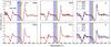Fig. 1 Spectra of images A (black) and D (red) in the spectral range 1300–1700 Å, covering the Si iv-C iv  lines. The left and middle panels show the spectra as observed in 1989, 1993, 2000, and 2011, after normalization to unity in the continuum. The three shaded areas correspond to regions where the absorption changed significantly over the past 20 years, as discussed in Sect. 3.2. The top and bottom right panels show the change of intrinsic absorption over time for images A and D.

Our analysis focuses on the microlensing in image D, which is compared to image A. The latter image did not show evidence for significant microlensing in the rest-frame UV wavelength range, over the last ten years (Paper I), and the current data confirm this finding. Although the intrinsic variability of H1413+117 is relatively small, ambiguity between differences caused by intrinsic variability and microlensing can be present. Fortunately, our new spectra have been obtained at two epochs separated by 25 days, matching the time delay Δt = 23 ± 4 days between images A − D (Goicoechea & Shalyapin 2010; Rathna Kumar et al. 2015). Unless otherwise stated, when we present spectra of A and D in the (rest-frame) UV range, we use the spectra separated by the time delay, namely the spectrum of A obtained on 2011-03-05 and that of D obtained on 2011-03-31.

3.1. Methodology

We follow two complementary methods to characterize the microlensing signal. On the one hand, the amplitude of microlensing as a function of wavelength is measured using the “MmD” decomposition technique (Sluse et al. 2007, 2012a; Hutsemékers et al. 2010; Braibant et al. 2014), briefly summarized hereafter (Sect. 3.1.1). On the other hand, measurement of microlensing in the C iv  absorption trough, is realized by calculating the equivalent width (EW) of the absorption line over small velocity slices (Sect. 3.1.2).

3.1.1. The MmD

Assuming that the observed spectra F_i of the lensed image i is the sum of a spectrum F_M, which is only macrolensed, and of a spectrum F_Mμ, which is both macro- and microlensed, it is possible to extract components F_M and F_Mμ using pairs of observed spectra. Indeed, considering a line profile, we can write $\begin{array}{ccc}{\mathit{F}}_{\mathrm{1}}& \mathrm{=}& \mathit{M}{\mathit{F}}_{\mathit{M}}\mathrm{+}\mathit{M\mu }{\mathit{F}}_{\mathit{M\mu }}\\ {\mathit{F}}_{\mathrm{2}}& \mathrm{=}& {\mathit{F}}_{\mathit{M}}\mathrm{+}{\mathit{F}}_{\mathit{M\mu }}\mathit{,}\end{array}$where M = M₁/M₂ is the macroamplification ratio between images 1 and 2 and μ the microamplification factor of image 1. We assume that image 2 is not affected by microlensing. We can conveniently rewrite these equations to isolate the components of interest: $\begin{array}{ccc}{\mathit{F}}_{\mathit{M}}& \mathrm{=}& \frac{\mathrm{-}\mathit{A}}{\mathit{A}\mathrm{-}\mathit{M}}\left(\frac{{\mathit{F}}_{\mathrm{1}}}{\mathit{A}}\mathrm{-}{\mathit{F}}_{\mathrm{2}}\right)\mathit{,}\\ {\mathit{F}}_{\mathit{M\mu }}& \mathrm{=}& \frac{\mathit{M}}{\mathit{A}\mathrm{-}\mathit{M}}\left(\frac{{\mathit{F}}_{\mathrm{1}}}{\mathit{M}}\mathrm{-}{\mathit{F}}_{\mathrm{2}}\right)\mathit{,}\end{array}$where A = Mμ. Up to a scaling factor, F_M only depends on A, while F_Mμ only depends on M. A is the scaling factor between the F₁ and F₂ continua. It can be accurately determined as the value for which F_M(A) = 0 in the continuum. The microamplification factor of the continuum is then estimated using μ = A/M.

For the MmD of images A and D presented hereafter, we fix M = 0.40 ± 0.02 prior to the decomposition (instead of the empirical determination performed in earlier papers). This value is consistent with values retrieved around H β + [O iii] with SINFONI data (Paper I, M = 0.38 ± 0.01), and with the mid-IR flux ratios obtained by Mac Leod et al. (2009; M = 0.40 ± 0.06).

3.1.2. The equivalent width

The EW, because it involves a normalization by the continuum, is a simple method to unveil differential microlensing between the continuum and another source of emission. By definition, the equivalent width of a line (in emission or absorption) is $\mathit{EW}\mathrm{=}{\mathrm{\int }}_{{\mathit{\lambda }}_{\mathrm{1}}}^{{\mathit{\lambda }}_{\mathrm{2}}}\left(\mathrm{1}\mathrm{-}\frac{{\mathit{F}}_{\mathit{\lambda }}}{\mathrm{ℱ}}\right)\hspace{0.17em}\mathrm{d}\mathit{\lambda ,}$(5)where ℱ is the continuum intensity underlying the absorption or emission line and usually approximated by the continuum emission on either side of the studied feature. The flux over the wavelength range of interest [λ₁,λ₂] is denoted F_λ. It is easy to see that the EW is only modified due to microlensing if F_λ and ℱ are microlensed at different levels, i.e., if the microlensed fluxes are ℱ′ = μ_cℱ, and ${\mathit{F}}_{\mathit{\lambda }}^{\mathrm{\prime }}\mathrm{=}{\mathit{\mu }}_{\mathit{\lambda }}{\mathit{F}}_{\mathit{\lambda }}$, the EW only changes if μ_λ ≠ μ_c.

3.2. Microlensing around the C IV line

First, we focus on the region of the C iv λ1549 line. Figure 1 shows the variations observed in images A and D between 1989 and 2011. The visual inspection of the spectra, normalized in the spectral range 1445–1455 Å, free of line emission, shows that the two spectra do not match, and, in particular, the flux in the emission lines (e.g., the peaks of the C iv  and Si iv-O iv) is smaller in image D than in A. This has been observed previously and is caused by microlensing amplification of the continuum of image D. Indeed, because we have normalized the spectra in the continuum region, the magnification of the continuum of D leads to an apparently less intense emission line in that image, because the line is actually unaffected by microlensing.

The other important feature to notice in Fig. 1, is the difference of absorption depth in A and D on the blue side of C iv. This is particularly noticeable in the range 1455–1505 Å, delimited with three shaded areas, and where the absorption is less deep. On the one hand, we see a decrease of the depth of the absorption with time. This corresponds to a long-term intrinsic decrease of the absorption. On the other hand, we observe a relative change of the absorption in A and D over time: prior to 2000, the absorption is deeper in image D than in A; in 2000, it is similar in A and D; and finally in 2011, it is deeper in image A. Because of this inversion of the relative absorption between A and D in 2011, at that epoch it is impossible to perform a MmD with a zero continuum everywhere in F_M, as shown in Fig. 2. Indeed, when we enforce the continuum to be zero in F_M, setting μ = 1.75, we violate the positivity constraint on F_M at the level of the absorber in the blue side of the C iv line (see light gray line in Fig. 2). In order to get F_M = 0 in that range, it is necessary to allow for a larger amount of microlensing of the continuum: μ = 2.0 (F_M shown with a thick black line in Fig. 2). This new value of μ yields F_M > 0 in the unabsorbed continuum flux. At the same time, a large fraction of the continuum flux is still visible in F_Mμ (i.e., the continuum emission above the dotted line in Fig. 2). Therefore, the MmD suggests that there are two components producing the continuum, one originating from a region, which is sufficiently compact to be microlensed, visible in F_Mμ, and another one that we detect in F_M, and which comes from a nonmicrolensed, and, hence, more extended region. We emphasize that this detection of an extended continuum emission with the MmD also implies that the compact and the extended continua are differently absorbed. More specifically, the extended continuum has to be more absorbed than the compact continuum (in the range 1455–1505 Å). As explained in Appendix A, if both continua were similarly absorbed by the outflowing gas, or if the most compact region was more absorbed than the extended region, the flux from the latter would remain undetected with the MmD when imposing F_M = 0 at the wavelength of the C iv  absorber (i.e., λ ~ 1500 Å). On the other hand, we may not exclude larger magnification of the compact continuum. Figure 2 shows the decomposition for μ = 2.5 (top gray line). In that case, the intensity of the extended continuum emission equals the intensity of the compact (microlensed) continuum.

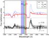Fig. 2 MmD performed on images A and D of H1413+117 in 2011, using M = 0.4 (Sect. 3.3). The dashed blue line is the flux of image A. The thick black line is the fraction of the flux FM unaffected by microlensing for μ = 2.0. The red line is the corresponding microlensed fraction of the flux FMμ (shifted up to ease legibility), the dotted horizontal line is the line corresponding to FMμ = 0. The gray lines show the decomposition for two other values of μ (see Sect. 3.2). The three shaded areas correspond to the three regions A1 − A3 as discussed in the text.

To better characterize this differential signal in A and D, we show in Fig. 3 the time variation of the EW of the absorption in three different wavelength ranges (Figs. 1 and 2): the range A1 = [1496, 1505] Å ([–10 274, –8532] km s^-1), is a flat absorption plateau, which barely changes profile over time, but whose depth is significantly decreasing; the range A2 = [1482, 1496] Å ([–12 984, –10 274] km s^-1) covers the highest velocity part of the absorption as observed in 2011; and finally A3 = [1455, 1482] Å ([–18 209, –12 984] km s^-1) is the range where absorption was detected prior to 2011. The variation of EW, shown in Fig. 3, allows us to assess the significance of the relative absorption differences detected in Fig. 1. The EW declines over the 22 years time span of the observations, in agreement with the intrinsic decrease of the absorption depth seen in Fig. 1. In addition, while EW_A<EW_D before 2000, the reverse behavior is detected in 2011. The observed differences of EW in A1 and A2 are highly significant. We demonstrate in Appendix B that it is only possible to observe EW_A > EW_D in presence of two sources of continuum light, which are differently absorbed and microlensed. The difference of EW observed between A and D at other epochs can also be understood under this hypothesis, but in that case the interpretation is not unique, as EW_A<EW_D can also be explained by superimposed broad line emission at the wavelength of the absorber.

To summarize, the MmD decomposition and the EW variation reveal the existence of two sources of continuum, a compact continuum that is microlensed, and a continuum that is more extended, and hence not microlensed. The MmD reveals the extended continuum in a visual and intuitive way, while the EW allows us to assess the significance of the observed signal.

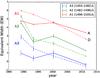Fig. 3 Time variation of the equivalent width of the absorption, in the wavelength ranges A1–A3 (see legend), for image A (solid) and D (dashed).

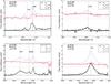Fig. 4 MmD for Ly α +N v (top left), C iii] (top right), H β (bottom left), H α (bottom right) emissions. The values of A = M × μ derived for each line are based on the individual frames, while the MmD is shown for the sum of the individual spectra.

3.3. Microlensing around other lines: chromatic microlensing

The spectra obtained in 2011 cover a large fraction of the wavelength range [1100, 7000] Å  (rest frame). Using the MmD technique (Sect. 3.1.1), we can derive the amplitude of microlensing as a function of wavelength. Because of the lack of apparent chromaticity of M empirically measured in past optical and NIR spectra (Paper I), we may assume that there is no significant differential extinction between A and D¹. The measurement of the amplitude of microlensing, in the vicinity of the main emission lines, is repeated for each individual spectra. The standard deviation between measurements (from three spectra for FORS2 data and four spectra for SINFONI) is quadratically added to the uncertainty in the relative flux calibration between epochs (UV data), and used to calculate the standard error on the mean. The results of this procedure are summarized in Table 1. The MmD of the main emission lines is presented in Fig. 4. As explained above, the measurements in the rest-frame UV account for the time delay. Although intrinsic variability of the absorption lines is noticeable between the two epochs, it mostly affects the value of μ derived from C iv. In that case, measurements of μ on spectra obtained at a single epoch nevertheless agree at the 3σ level with those presented in Table 1. We may then be confident that the values of μ derived at a single epoch from the Hβ and Hα lines are accurate, in particular, since they are identical within the errors to those derived in Paper I.

The extended continuum detected around C iv (Sect. 3.2) is also tentatively detected around Ly α -N v. In that case, the evidence for an extended continuum flux is set by the absorbers in the range [1170–1190] Å (rest frame), which have been identified as H i absorption at z ~ 2.4 − 2.45 (line number 48 to 51 in Monier et al. 1998). They are therefore likely to be high velocity absorptions associated with H1413+117. Note that in the MmD of the Ly α line shown in Fig. 4, the positivity constraint in F_M is (marginally) violated around λ ~ 1165 Å. This is acceptable because this absorption feature is due to intervening C iv (line number 45, 46 in Monier et al. 1998), and therefore may be intrinsically different in A and D. On the other hand, the absorption in the blue side of O iv-Si iv sets almost no constraint on the presence of an extended continuum in that wavelength range. This is because the well-identified high velocity absorption A1 − A2, visible in C iv, is shallower and less clearly detected, in the O iv-Si iv blend.

3.4. Differences of light paths between images

Up to now, we have shown that the continuum flux from H1413+117 originates from two regions, a compact one, which is small enough to be microlensed, and a more extended one, which is not microlensed. An alternative interpretation could be that significant inhomogeneities of the outflowing absorbing material lead to different absorption for each of the lensed images. This can be tested by estimating the linear comoving separation between the two different lensed images A and D as a function of the distance to the central black hole. The comoving linear beam separation for z>z_lens (Smette et al. 1992; Chartas et al. 2007) is given by 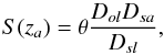$\mathit{S}\mathrm{\left(}{\mathit{z}}_{\mathit{a}}\mathrm{\right)}\mathrm{=}\mathit{\theta }\frac{{\mathit{D}}_{\mathit{ol}}{\mathit{D}}_{\mathit{sa}}}{{\mathit{D}}_{\mathit{sl}}}\mathit{,}$(6)where θ is the separation between the lensed images, D is the angular diameter distance, and the subscripts o, l, s, a refer to the observer, lens, source, and absorber, respectively.

In order to see if the comoving distance between light paths is larger than a cloud size, we need to assume a reasonable cloud distance to the central engine. Important constraints on the distance and geometry of absorbing troughs have been set by variability studies of BALs. Two scenarios are generally considered. One explaining the variability as caused by rapid crossing of an absorbing cloud, and one as a rapid change of ionization in the ionized material (e.g., Lundgren et al. 2007; Filiz Ak et al. 2012; Capellupo et al. 2013; Wildy & Goad 2015; Grier et al. 2015). Recently, Capellupo et al. (2014) carried out a detailed study of the variability of the A1–A2 absorbers in H1413+117. Based on the comparison of the C iv and P v absorptions, they showed that the C iv absorption is saturated such that its variability is most likely caused by rapid crossing of an absorbing cloud. Assuming a so-called crossing-disc model, they derive an upper limit of 3.5 pc on the radial distance of the cloud to the black hole. At this distance, the separation between A and D corresponds to a linear beam separation of 3.2 × 10¹³ cm, (10^-5pc) hence about ten times smaller than the gravitational radius of the source, ensuring that the two lines of sight cross the same absorber. Therefore, the possibility that the light from image A and D intercept different clouds (or regions of a cloud with different opacities) is very unlikely.

4. Characteristics of the extended continuum

In this section, we first try to characterize some of the properties of the extended continuum, in particular its wavelength dependence, and its possible time variability. We then discuss its origin.

4.1. Wavelength dependence

The MmD yields the measurement of the relative fractions of compact (cc) and extended (ce) continua from the total flux. If we define f as the fraction of the total continuum flux ℱ = F_cc + F_ce, which is extended (i.e., f = F_ce/ ℱ), we find based on the MmD around C iv and Ly α that f = 0.3 (i.e., 30% of the total flux is nonmicrolensed). This value of f implies that F_ce/F_cc = f/ (1 − f) = 0.42. Larger values of f may be acceptable (Sect. 3.2, Fig. 2).

Although we do not observe a significant difference of the amount of extended continuum between the Ly α and C iv wavelengths, we cannot exclude a small chromatic change. Since the Ly α and C iv absorbers used to derive μ correspond to clouds at different velocities, the opacity of the absorber (i.e., τ_cc and τ_ce, Appendix A) may be different in Ly α and C iv, leading to a coincidentally similar measure of μ around those two lines, but the effect is unlikely to be large. At wavelengths redder than C iv, the situation is more complex as the lack of intrinsic absorption in that range precludes the detection of the extended continuum. At the wavelength of the Balmer lines in the NIR, we measure μ ~ 1.5, both in 2005 and 2011. This constancy of the amplitude of microlensing suggests that the contribution from a nonmicrolensed continuum is negligible in the redder part of the spectrum (i.e., λ > 4800 Å) because the extended continuum is stronger in 2011 than in 2005 (Sect. 4.2). Consequently, we consider in the following analysis that there is no contribution of the extended continuum at those wavelengths.

4.2. Temporal variation

Our detection of an extended continuum in 2011 has been possible owing to the microlensing of image D and to the differential absorption of the compact and extended continua in 2011, the extended continuum being more absorbed than the compact continuum. We may wonder whether the extended continuum was present at earlier epochs, or simply could not be detected because of the time variation of the relative absorption, an insufficient signal-to-noise ratio in past data, and/or changes of the microlensing configuration. Actually, the MmD presented in Fig. 6 of Paper I shows that F_M < 0 in part of the A2 − A3 absorption for the data obtained in 2000. Our Fig. 3 also reveals that EW_A > EW_D for A2 and A3 in 2000, confirming (at least from A2) a significant detection of the extended continuum at that epoch. Accounting for this absorption in the MmD (i.e., enforcing F_M = 0 at the location of the absorber) leads to F_ce/F_cc ~ 20% and to μ ~ 2.0 ± 0.12. Although the detection is more noisy, this suggests that the extended continuum was indeed present in those data but with a smaller contribution. At earlier epochs, we also detect differences of EW between A and D but with EW_D > EW_A. Although this is not an unambiguous signature of an extended continuum since emission from the BLR can also explain this signal (see Appendix B), it is plausible to attribute the origin of this difference of EW to the extended continuum. Contrary to the situation observed in 2000 and 2011, the extended continuum has to be less absorbed than the compact one (Appendix B). Because we do not know the optical depth of the gas covering the compact and extended continua, we cannot derive F_ce/F_cc with the MmD or based on the EW prior to 2000.

Another way to approach the issue of time variability of F_ce/F_cc is to look at the variation of the effective amplitude of microlensing over time. When calculating μ′ determined by making F_M = 0 in the unabsorbed continuum adjacent to C iv (see Appendix A), we find it to be roughly constant in 1993/ 2000/2005 (μ′ ≃ 2.0 ± 0.2, Paper I). In 2011, μ′ significantly drops to 1.75 ± 0.07. Under the hypothesis that the amplitude of microlensing does not significantly change with time, this indicates that a decrease of μ′ results from an increase of F_ce/F_cc (i.e., Eq. (A.5)). When we only measure the amplitude of microlensing for the compact continuum (i.e., allowing F_M ≠ 0, cf. Appendix A), we find μ = 2.0 ± 0.1 in 2011 (Table 1), which is consistent with the amplitude of microlensing in 1993/2000/2005. Moreover, the micromagnification μ of the H β continuum did not change between 2005 and 2011, also supporting the constancy of μ in the last decade. This absence of variation of the microlensing signal agrees with the small relative transverse velocity of the lens in H1413+117 (Mosquera & Kochanek 2011).

In summary, we find evidence for extended continuum in the past data, but the data also suggest that the fraction of extended over compact continuum varies with time.

4.3. A physical model

The extended continuum unveiled by our data may simply be genuine flux from the host galaxy, or scattered emission by the host, similar to that unveiled by Borguet et al. (2008) in Type 1, and by Zakamska et al. (2006) in Type 2 AGNs. This interpretation is however very unlikely. Indeed, we have shown that at least 30% of the total continuum emission is extended. However, H1413+117 is a BAL quasar, and most of the light is occulted by the optically thick absorption in the blue wing of C iv, with no more than a few percent of the flux detected at those wavelengths. Although this absorber is at least at the distance of the BLR (because it occults the C iv emission), it is unlikely to cover the whole host galaxy.

Broad absorption line quasars like H1413+117 are known to be intrinsically polarized because of scattering of the continuum flux in an extended region possibly located at a radius comparable to the BLR radius or in a polar wind (Lamy & Hutsemékers 2004; Schmidt & Hines 1999). It is legitimate to postulate that the same region is at the origin of the polarization and the source of extended continuum, especially since the observed fraction of extended continuum is consistent with the polarization degree observed in H1413+117 (Hutsemékers et al., in prep.). The scattering could be caused by dust, or by electrons. If dust is responsible for the scattering, we expect a wavelength dependence of the extended continuum as λ^-4. This is consistent with the apparent absence of extended continuum in H β, but implies an extended continuum emission 2.7 times stronger at the level of Ly α than around C iv. Another possibility is scattering by electrons. This does not yield a chromatic dependence of the extended continuum, in agreement with our observation in the blue. Under this scenario, it remains to be seen how we can explain the lack of extended continuum at the reddest wavelengths, e.g., around H β and H α. A combination of both dust and electron scattering is also possible.

Alternatively, to explain the UV peak in quasar spectral energy distribution (and other inconsistencies between the standard disc model and the SED of quasars), Lawrence (2012) has proposed the existence of a population of dense clouds, which partly reprocesses the intrinsic continuum from the accretion disc. A false continuum is produced in the UV coming from an extended source. Since these clouds mostly reflect the inner continuum through electron scattering, we expect the ratio of the two continua to be roughly constant in the Ly α-C iv spectral range, in agreement with our observations. This model also predicts a decrease of the fraction of extended continuum at reddest wavelength, compatible with the absence of significant extended continuum around H β. In addition, in that model, UV variability is interpreted as changes of the cloud covering factor. It can occur independently of variations of the intrinsic continuum and can explain the change of F_ce/F_cc between 2000 to 2011 (Sect. 4.2). In this model, the pseudocontinuum flux is suspected to originate from cold clouds located at about 30 R_Sch (Schwarchild radii) from the continuum, which corresponds to a distance of 0.037 pc = 1.16 × 10¹⁶ cm ~0.6 η₀ (for log (M_BH/M_⊙) = 9.12, and ⟨M⟩ = 0.3 M_⊙ in Eq. (7)). Even if the clouds were located in the range 30 − 100 R_Sch, the extended pseudocontinuum would be of the order of 1–2 η₀, and would therefore be sensibly microlensed.

In conclusion, we can rule out the host galaxy as the source of the extended continuum. Instead, we postulate that the latter is scattered light by dust or electrons. Scattering by dust or electrons could take place in the same region as that at the origin of the polarization in BAL quasars. Dust scattering yields a chromatic dependence, while electron scattering does not. Therefore, dust may explain the apparently small amount of extended continuum at the wavelength of H β, but implies that we underestimate the contribution of the extended continuum at the level of Ly α by almost a factor 3. Variations of microlensing and of the absorption in front of C iv and Ly α may possibly help to test this scenario. Simple electron scattering fails to explain the decrease of extended continuum at redder wavelengths. The model of blurred reflection of the continuum proposed by Lawrence (2012) accounts for most of the observational properties of the extended continuum we detect, except that the cold clouds responsible for the “continuum-reflection” are expected to be located too close to the black hole to remain unaffected by microlensing.

5. Constraints on the accretion disc parameters

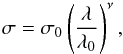
We now use our measurements of the chromatic microlensing (Sect. 3.3) to derive the size of the compact continuum (which originates from the accretion disc) as a function of wavelength. Following various other works (e.g., Eigenbrod et al. 2008; Bate et al. 2008; Anguita et al. 2008), we test an accretion disc model with a temperature profile T ∝ R^{−1 /ν}. This kind of model leads to a dependence of the source size σ as a function of wavelength σ ∝ λ^ν. This model has two parameters, the source size σ (converted into the half-light radius R_1/2) and the power-law index ν, for which we derive the probability density function (PDF), following the Bayesian scheme described hereafter (Sect. 5.1).

5.1. Methodology

To turn the chromatic variation of microlensing into a quantitative information on the disc, we need to compare this signal to microlensing simulations calculated for different sizes and temperature profiles of the accretion disc, as well as for different fractions of compact objects in the lensing galaxy. The data to which the microlensing simulations are compared are the measurements presented in Table 1, excluding μ measured from C iii] and Si iv due to the uncertainty in the fraction of extended continuum at those wavelengths. It is important to keep in mind that those values of μ are derived assuming that the fraction of flux from the extended continuum equals the minimum value needed to reproduce our data (i.e., F_ce/F_cc = 0.42, Sect. 4.1).

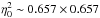
We follow a Bayesian scheme similar to that developed in Bate et al. (2008). Throughout the analysis, the sizes are expressed in units of microlensing Einstein radius η₀, i.e., 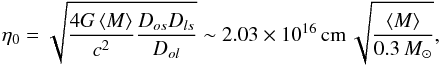${\mathit{\eta }}_{\mathrm{0}}\mathrm{=}\sqrt{\frac{\mathrm{4}\mathit{G}⟨\mathit{M}⟩}{{\mathit{c}}^{\mathrm{2}}}\frac{{\mathit{D}}_{\mathit{os}}{\mathit{D}}_{\mathit{ls}}}{{\mathit{D}}_{\mathit{ol}}}}\mathrm{~}\mathrm{2.03}\mathrm{\times }{\mathrm{10}}^{\mathrm{16}}\hspace{0.17em}\mathrm{cm}\hspace{0.17em}\sqrt{\frac{\mathrm{⟨}{\mathit{M}}_{\mathrm{⟩}}}{\mathrm{0.3}\hspace{0.17em}{\mathit{M}}_{\mathrm{\odot }}}}\mathit{,}$(7)where ⟨M⟩ is the average mass of the stars in the lensing galaxy. The different steps of our analysis can be summarized as follows:

• i)

  We use the inverse ray-shooting code of Wambsganss (1998) to generate microlensing magnification pattern of 100 × 100${\mathit{\eta }}_{\mathrm{0}}^{\mathrm{2}}\mathrm{~}\mathrm{0.657}\mathrm{\times }\mathrm{0.657}$ pc². We fix the value of the local convergence and shear at the location of image D to (κ,γ) = (0.576,0.68) (Pooley et al. 2012), and calculate maps for ten different fractions f_∗ of the total matter density in form of compact objects, logarithmically distributed in the range f_∗ ∈ [0.01,1]. Because of the small dependence of microlensing properties on the mass function of microlenses (Lewis & Irwin 1996; Kochanek 2004), we assume that all the microlenses have the same mass. We then convolve the maps with the luminosity profile of the source. We model the disc as a two-dimensional Gaussian profile. The exact shape of the profile has little influence on the results (Mortonson et al. 2005), provided that profiles with the same half-light radius R_1/2 are considered. We consider 51 logarithmically distributed half-light radii R_1/2 ∈ [0.025,2.5] η₀.

• ii)

  We generate a list of 2 × 10⁶ random positions to be extracted from the maps, excluding 500 pixels (5η₀) at the border of the map.

• iii)

  Based on those positions, we extract the magnification for each source size, and construct a chromatic curve representing the magnification as a function of the source size.

• iv)

  The wavelength of observations λ, and size of the source are related through the equation $\mathit{\sigma }\mathrm{=}{\mathit{\sigma }}_{\mathrm{0}}{\left(\frac{\mathit{\lambda }}{{\mathit{\lambda }}_{\mathrm{0}}}\right)}^{\mathit{\nu }}\mathit{,}$(8)where σ₀ is the disc size (in practice, the width of a Gaussian profile) at the reference wavelength λ₀. This relation enables us to transform the dependence of the amplitude of microlensing with the size of the source into a wavelength dependence of the microlensing signal. 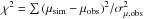We compare each simulated microlensing light curve to the data, and calculate a ${\mathit{\chi }}^{\mathrm{2}}\mathrm{=}\sum \mathrm{(}{\mathit{\mu }}_{\mathrm{sim}}\mathrm{-}{\mathit{\mu }}_{\mathrm{obs}}{\mathrm{)}}^{\mathrm{2}}\mathit{/}{\mathit{\sigma }}_{\mathit{\mu ,}\mathrm{obs}}^{\mathrm{2}}$, where the sum is over all the observed wavelengths, and σ_μ,obs is the uncertainty in the estimated microlensing magnification at each wavelength. When necessary, we perform linear interpolation of the simulated microlensing signal to derive the amplitude of microlensing at the wavelength of the observations.

• v)

  We calculate the likelihood of each pair of parameters (σ,ν), via summing the likelihood of each light curve estimated as L_i(F_obs | σ,ν,f_∗) = exp( − χ²/ 2). This enables us to derive, for each fraction of compact matter f_∗, a two-dimensional map of the likelihood of the source parameters.

• vi)

  We perform a weighted sum of the likelihoods associated with each f_∗, using the dark matter probability distribution derived by Pooley et al. (2012), based on the study of the X-ray microlensing in the system. We then convert the likelihood into probability distribution using the Bayes theorem.

5.2. Results

The 2D probability density function d²P/(dR_1/2 dν) resulting from our analysis is shown in Fig. 5. This PDF is marginalized over the fraction of compact objects f_∗ in the lensing galaxy, weighted by the dP/df_∗ estimated by Pooley et al. (2012). Our most likely values of the disc size and power-law index of the temperature profiles are ${\mathit{R}}_{\mathrm{1}\mathit{/}\mathrm{2}}\mathrm{(}{\mathit{\lambda }}_{\mathrm{0}}\mathrm{=}\mathrm{0.18}\hspace{0.17em}\mathit{\mu }\mathrm{m}\mathrm{)}\mathrm{=}\mathrm{0.3}\hspace{0.17em}{\mathit{\eta }}_{\mathrm{0}}\mathrm{=}\mathrm{6.1}\mathrm{\times }{\mathrm{10}}^{\mathrm{15}}\hspace{0.17em}\sqrt{⟨\mathit{M}⟩\mathit{/}\mathrm{0.3}\hspace{0.17em}{\mathit{M}}_{\mathrm{\odot }}}$ cm = 0.00197 $\sqrt{⟨\mathit{M}⟩\mathit{/}\mathrm{0.3}\hspace{0.17em}{\mathit{M}}_{\mathrm{\odot }}}$  pc, and ν = 0.4. However, those values significantly depend on our prior on the fraction of compact objects. This is illustrated in Fig. 6, where we show the PDF for R_1/2 at a fixed value of ν = 4/3 (i.e., the standard accretion disc value), and for various amounts of the compact matter fraction f_∗. Those PDFs are compared to the case where we use the prior on f_∗ from Pooley et al. (2012, i.e., as in Fig. 5).

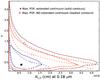Fig. 5 Probability distribution for the size of the disc R1/2, and for the power-law index ν of the temperature profile. Solid contours correspond to the constraints obtained after correction of the microlensing amplitude for the presence of an extended continuum, and the dashed contours show the constraints if we do not account for the extended continuum. Contours are 68.3, 95.5, and 99.7% confidence level. The corresponding peaks of the probability distribution are shown as a filled black star and red cross, respectively.

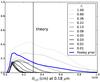Fig. 6 PDF of the source size for a standard accretion disc model (ν = 4/3) and various fractions of compact objects f∗ (extreme values f∗ = 1, shown in light gray, and f∗ = 0.01, shown in dark gray, correspond to 100% and 1% of the total matter being compact, respectively). The thick blue line is the result obtained assuming the same prior on f∗, as in Fig. 5, namely the prior resulting from the analysis of Pooley et al. (2012). The vertical solid line is the theory size for a Shakura-Sunyaev model based on Eq. (10) for cos(i) = 0.5 (R1/2 ~ 3.04 × 1015 cm ~10-3 pc).

Our size estimates can be compared to expectation from theory. The radius R_λ at which the disc temperature equals the photon energy, kT = hc/λ_rest is given by the following expression (Poindexter & Kochanek 2010; Blackburne et al. 2011): 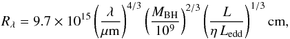${\mathit{R}}_{\mathit{\lambda }}\mathrm{=}\mathrm{9.7}\mathrm{\times }{\mathrm{10}}^{\mathrm{15}}{\left(\frac{\mathit{\lambda }}{\mathit{\mu }\mathrm{m}}\right)}^{\mathrm{4}\mathit{/}\mathrm{3}}{\left(\frac{{\mathit{M}}_{\mathrm{BH}}}{{\mathrm{10}}^{\mathrm{9}}}\right)}^{\mathrm{2}\mathit{/}\mathrm{3}}{\left(\frac{\mathit{L}}{\mathit{\eta }\hspace{0.17em}{\mathit{L}}_{\mathrm{edd}}}\right)}^{\mathrm{1}\mathit{/}\mathrm{3}}\mathrm{cm}\mathit{,}$(9)where η is the accretion efficiency (assumed to be η = 0.1), M_BH the black hole mass, and L_edd is the Eddington ratio. An alternative expression for the size which depends only on the magnification corrected luminosity can also be derived (Morgan et al. 2010; or based on T_eff and Ṁ in Davis & Laor 2011 and Laor & Davis 2014): 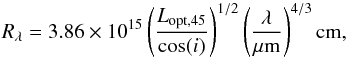${\mathit{R}}_{\mathit{\lambda }}\mathrm{=}\mathrm{3.86}\mathrm{\times }{\mathrm{10}}^{\mathrm{15}}{\left(\frac{{\mathit{L}}_{\mathrm{opt}\mathit{,}\mathrm{45}}}{\cos \mathrm{\left(}\mathit{i}\mathrm{\right)}}\right)}^{\mathrm{1}\mathit{/}\mathrm{2}}{\left(\frac{\mathit{\lambda }}{\mathit{\mu }\mathrm{m}}\right)}^{\mathrm{4}\mathit{/}\mathrm{3}}\mathrm{cm}\mathit{,}$(10)where L_opt,45 is the luminosity at 4861 Å in units of 10⁴⁵ erg s^-1 cm^-2, and i is the inclination of the disc. Figure 6 shows that the theory size (with L_opt,45 = 5.22; Sluse et al. 2012b) is somewhat larger than the microlensing size (using ⟨M⟩ = 0.3 M_⊙ in Eq. (7)). The presence of an extended continuum only has a small impact on this result. If we repeat our analysis using microlensing factors derived by forcing F_M = 0 in the continuum (e.g., μ′ = 1.75 in Fig. 1, see also Appendix A), we then find the PDF represented by the dashed contours in Fig. 5, which peaks at (R_1/2,ν) = (0.37 η₀,0.2).

Because we cannot exclude that the amplitude of microlensing in the compact continuum is larger than the value used above (for F_ce/F_cc ~ 0.4), we experimented with two alternative hypotheses for the chromatic behavior of the extended continuum (Sect. 4.1). On the one hand, we assumed that in the blue (i.e., up to C iv), F_ce/F_cc ~ 1, yielding an increase of the amplitude of microlensing in the blue, namely μ = 2.5 ± 0.12 for C iv  and μ = 2.56 ± 0.13 for Ly α. On the other hand, we considered a constant fraction of extended continuum observed from C iv to H α  (this yields an increase of the amplitude of microlensing μ ~ 2 around H β  and H α). The most likely sizes derived for those alternative signals fell within the 1σ solid contours of Fig. 5. We can then conclude that our estimates of R_1/2 and ν are robust within a factor 2 with respect to F_ce/F_cc, and that the strongest source of error is the prior on f_∗.

5.3. Discussion

In recent years, microlensing studies based on significant samples of microlensed quasars found that the size of the accretion disc is larger by a factor 2 to 10 than the theory size derived from Eq. (9) (Morgan et al. 2010; Blackburne et al. 2011; Jiménez-Vicente et al. 2012; and see Hall et al. 2014 for a summary). Our snapshot (i.e., single epoch) microlensing measurement of H1413+117 instead favors a most likely half-light radius smaller than the theoretical prediction, although the upper limit of the confidence interval extends to about two times the theory size (99.7% C.I.; Fig. 6). There is therefore no tension between the disc size that we measure in H1413+117  and that measured in other systems. More interesting is the impact of the presence of an extended continuum amounting to 30% of the total flux. Figure 5 shows that the disc size shrinks by typically 20% when we account for the extended continuum. Morgan et al. (2010) and Dai et al. (2010) reached similar conclusions, assuming that 30% of the broadband flux in lensed quasars comes from regions of larger physical extent than the compact continuum.

The other constraint provided by our data regards the power-law index of the disc temperature profile. We find a most likely index, ν = 0.4, which is significantly smaller than that of the standard accretion disc, ν = 4/3 (Fig. 5). Nevertheless, the latter is compatible with our data within 2σ, as generally found for measurements based on single epoch data (e.g., Bate et al. 2008; Floyd et al. 2009). Our result also agrees with the finding of Blackburne et al. (2011) that microlensing measurements support a steeper temperature profile than in the standard model. Again, we should underline the rather small impact of the extended continuum on those results. Conversely, the fraction of compact objects in the lens does play an important role on the parameter estimates. As suggested by Fig. 6, our data are more easily reproduced by a standard disc for higher values of f_∗, although a large fraction of compact objects is not favored by X-ray microlensing studies of H1413+117 (Pooley et al. 2012).

In summary, the extended continuum emission is not sufficient to explain discrepancies generally found between the standard accretion disc model and the microlensing measurements, however, we emphasize the important role played by the prior on the dark matter fraction on size measurements. Dark matter fraction estimates result from analyses, which generally assume the size of the source. Jiménez-Vicente et al. (2015) has recently demonstrated that this assumption has a non-negligible effect on the derived dark matter fraction at the location of the lensed images. The common assumption of a very small source size (especially in the X-rays) in dark matter fraction inferences yields a fraction of mass in compact form (f_∗) smaller than what is found by accounting for the extended nature of the source. If we postulate that the prior on f_∗ from Pooley et al. (2012) is shifted to low values because of this source size effect, we then find that the most likely disc parameters derived from microlensing in H1413+117  are closer to those of the standard accretion disc model.

6. Conclusions

The technique of quasar microlensing, which consists of analyzing the deformation of gravitationally lensed quasar spectra produced by stars in a lensing galaxy, is a powerful tool for studying the structure of the accretion disc since it constrains the size of the microlensed emission. This method generally shows that the size of the accretion disc is significantly larger than the theory size (see Hall et al. 2014, for a good summary). In this work, we have analyzed new spectra (obtained in 2011) of the lensed images A and D of the cloverleaf H1413+117, a quadruple-imaged BAL system located at redshift z ~ 2.55. Because of the presence of absorption covering the source of continuum, and of the existence of microlensing in one of the lensed images, we have unveiled the presence of two sources of continuum: a compact continuum-emitting region that is small enough to be microlensed, and a spatially separated nonmicrolensed continuum-emitting region that accounts for about 30% of the total continuum in the UV rest-frame part of the spectra (namely 1000–3000 Å). Because this extended continuum is detected in the UV, and is absorbed by the broad absorption trough, we think that it may not come from the host galaxy, but from the innermost regions of the system (possibly as small as the quasar torus or the broad line region). This extended continuum may be scattered light reprocessed either in the same scattering region as that at the origin of the polarization in BAL quasars, or closer to the compact continuum source as in the model proposed by Lawrence (2012). A reanalysis of archive spectra, shows that this extended continuum was already present in the past 22 years, but was less prominent compared to the compact continuum.

Owing to our method of analysis of the spectra, we effectively deblended the compact continuum from the nonmicrolensed continuum. The amplitude of microlensing for the compact continuum, which we attribute to the accretion disc emission, decreases as the wavelength increases. We use this chromatic variation of the microlensing to derive the size and index of the temperature profile of the disc, assuming that the latter varies like T ∝ R^{−1 /ν} (where ν = 4/3 corresponds to the standard Shakura-Sunyaev value). For this purpose, we develop a Bayesian analysis scheme, which compares simulated microlensing signals for different source sizes and index ν to the observed amplitude of microlensing. This analysis yields a most likely half-light radius of the source of R_1/2 = 0.61 × 10¹⁶cm at 0.18 μm, and a most likely index ν = 0.4. The index is smaller than the prediction from the standard model of accretion, but remains compatible with the latter at the 2σ level. Fixing ν = 4/3, we find a disc size that is about four times smaller than the theory size, but still statistically compatible. There is therefore no evidence for a stronger discrepancy between theory and microlensing disc size in this BAL quasar compared to what is found in other systems.

To test whether the extended continuum emission could explain the tension between standard theory and microlensing results, we repeated our measurement using an effective amplitude of microlensing, which is the amplitude of microlensing measured including both the compact and the extended continuum. This is equivalent to the measurements performed for other systems, where extended continuum emission is not detected (even when present). As expected, this procedure yields an increase of the microlensing size, and a decrease of the index ν, but the change is not large enough to explain the large microlensing sizes that are commonly reported. We emphasize that another parameter of the analysis, the fraction of matter in compact form in the lensing galaxy, may play a more important role in the source size measurement than the presence of an extended continuum. This is especially true for lensed systems where a small fraction of matter in compact form is assumed in simulations.

Our detection of two spatially separated sources of continuum has been possible owing to differential absorption between the two sources of continuum, and to microlensing of the most compact continuum. The same method may be used in other BAL systems, but its guarantee of success depends on the exact location of the absorbers with respect to the central engine. Innovative methods need to be developed to answer the many open questions about this extended continuum such as: is it present in other quasars, and visible for all quasar types? How does this continuum emission vary with wavelength? Is the extended continuum scattered light by the BAL wind, by the dust torus, or by cold clouds inner to the BLR?

Online material

Appendix A: MmD with an absorbed extended continuum

We consider a line profile where absorption is present. We write $\begin{array}{ccc}{\mathit{F}}_{\mathrm{1}}& \mathrm{=}& \mathit{M}\hspace{0.17em}\mathrm{(}{\mathit{F}}_{\mathit{ee}}\mathrm{+}{\mathit{F}}_{\mathit{ce}}\hspace{0.17em}{\mathit{e}}^{\mathrm{-}{\mathit{\tau }}_{\mathit{ce}}}\mathrm{)}\mathrm{+}\mathit{M\mu }\hspace{0.17em}{\mathit{F}}_{\mathit{cc}}\hspace{0.17em}{\mathit{e}}^{\mathrm{-}{\mathit{\tau }}_{\mathit{cc}}}\mathit{,}\\ {\mathit{F}}_{\mathrm{2}}& \mathrm{=}& {\mathit{F}}_{\mathit{ee}}\mathrm{+}{\mathit{F}}_{\mathit{ce}}\hspace{0.17em}{\mathit{e}}^{\mathrm{-}{\mathit{\tau }}_{\mathit{ce}}}\mathrm{+}{\mathit{F}}_{\mathit{cc}}\hspace{0.17em}{\mathit{e}}^{\mathrm{-}{\mathit{\tau }}_{\mathit{cc}}}\mathit{,}\end{array}$where F_ce represents the flux from an extended source of continuum, which is only macrolensed as the emission line flux F_ee, F_cc ≠ 0 is the flux from the source of continuum compact enough to be microlensed, and τ_cc (τ_ce) is the optical depth of the absorber in front of cc (ce). Using these relations in Eqs. (3) and (4) with A = Mμ, we obtain $\begin{array}{ccc}{\mathit{F}}_{\mathit{M}}& \mathrm{=}& {\mathit{F}}_{\mathit{ee}}\mathrm{+}{\mathit{F}}_{\mathit{ce}}\hspace{0.17em}{\mathit{e}}^{\mathrm{-}{\mathit{\tau }}_{\mathit{ce}}}\mathrm{+}\hspace{0.17em}\frac{{\mathit{A}}^{\mathrm{\prime }}\mathrm{-}\mathit{A}}{{\mathit{A}}^{\mathrm{\prime }}\mathrm{-}\mathit{M}}\hspace{0.17em}{\mathit{F}}_{\mathit{cc}}\hspace{0.17em}{\mathit{e}}^{\mathrm{-}{\mathit{\tau }}_{\mathit{cc}}}\\ {\mathit{F}}_{\mathit{M\mu }}& \mathrm{=}& {\mathit{F}}_{\mathit{cc}}\hspace{0.17em}{\mathit{e}}^{\mathrm{-}{\mathit{\tau }}_{\mathit{cc}}}\mathrm{+}\hspace{0.17em}\frac{\mathit{M}\mathrm{-}{\mathit{M}}^{\mathrm{\prime }}}{\mathit{A}\mathrm{-}{\mathit{M}}^{\mathrm{\prime }}}\hspace{0.17em}\mathrm{(}{\mathit{F}}_{\mathit{ee}}\mathrm{+}{\mathit{F}}_{\mathit{ce}}\hspace{0.17em}{\mathit{e}}^{\mathrm{-}{\mathit{\tau }}_{\mathit{ce}}}\mathrm{)}\mathit{.}\end{array}$In these equations, A′ and M′ are parameters tuned to satisfy constraints on F_M and F_Mμ. The constraint F_Mμ = 0 at wavelengths where F_cce^−τ_cc = 0 and F_ee ≠ 0 can only be satisfied with M′ = M. If M is correctly estimated, F_Mμ = F_cce^−τ_cc ≥ 0 independently of the existence of a nonmicrolensed extended continuum.

In the absence of a nonmicrolensed extended continuum (i.e., F_ce = 0), making F_M = 0 at wavelengths where F_ee = 0 and τ_cc = τ_ce = 0 (i.e., in the unabsorbed continuum) gives A′ = A. In the presence of a nonmicrolensed extended continuum, making F_M = 0 in the unabsorbed continuum gives A′ ≠ A. In this case, F_M = F_ce (e^−τ_ce − e^−τ_cc) at wavelengths where the continuum is absorbed and F_ee = 0, which can result in either positive or negative values for F_M whether τ_ce<τ_cc or τ_ce > τ_cc, respectively. Making F_M ≥ 0 allows the detection of the extended continuum in the latter case (τ_ce > τ_cc), but A′ = A is derived only if e^−τ_ce = 0 at some wavelengths where F_ee = 0 and e^−τ_cc ≠ 0. Without absorption (i.e., τ_ce = τ_cc = 0), such a nonmicrolensed extended continuum would remain unnoticed.

Note that μ′ = A′/M, determined by making F_M = 0 in the unabsorbed continuum, can be seen as the average microamplification of the whole continuum source, while μ = A/M refers to the microamplification of the compact continuum source. They are related by 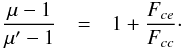$\begin{array}{ccc}\frac{\mathit{\mu }\mathrm{-}\mathrm{1}}{{\mathit{\mu }}^{\mathrm{\prime }}\mathrm{-}\mathrm{1}}& \mathrm{=}& \end{array}$(A.5)

Appendix B: Equivalent width in the absorption trough

In order to understand how microlensing affects the EW, we can write Eq. (5), with more explicit expression of F_λ and of the continuum flux ℱ. We assume that the latter is constant over the emission line and the absorption trough and is well approximated by the continuum flux measured in the vicinity of the line. We consider a broad emission line characterized by a flux F_λ,E, and a continuum originating from two regions, a compact region cc, compact enough to be microlensed, and a more extended region ce, which is not microlensed. We can specialize Eq. (5) in the presence of absorption. For a lensed image i, we obtain 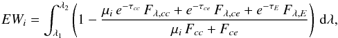$\mathit{E}{\mathit{W}}_{\mathit{i}}\mathrm{=}{\mathrm{\int }}_{{\mathit{\lambda }}_{\mathrm{1}}}^{{\mathit{\lambda }}_{\mathrm{2}}}\left(\mathrm{1}\mathrm{-}\frac{{\mathit{\mu }}_{\mathit{i}}\hspace{0.17em}{\mathit{e}}^{\mathrm{-}{\mathit{\tau }}_{\mathit{cc}}}\hspace{0.17em}{\mathit{F}}_{\mathit{\lambda ,cc}}\mathrm{+}{\mathit{e}}^{\mathrm{-}{\mathit{\tau }}_{\mathit{ce}}}\hspace{0.17em}{\mathit{F}}_{\mathit{\lambda ,ce}}\mathrm{+}{\mathit{e}}^{\mathrm{-}{\mathit{\tau }}_{\mathit{E}}}\hspace{0.17em}{\mathit{F}}_{\mathit{\lambda ,E}}}{{\mathit{\mu }}_{\mathit{i}}\hspace{0.17em}{\mathit{F}}_{\mathit{cc}}\mathrm{+}{\mathit{F}}_{\mathit{ce}}}\right)\hspace{0.17em}\mathrm{d}\mathit{\lambda ,}$(B.1)where μ_i is the amplitude of micromagnification of the compact continuum cc, and τ_cc, τ_ce, and τ_E are the optical depths of the gas absorbing the compact continuum, the extended continuum, and the broad emission line, respectively. Contrary to Appendix A, we make explicit the fact that the emission line can be absorbed (i.e., F_ee = e^−τ_EF_λ,E).

Equation (B.1) clearly shows that if F_λ,ce = F_λ,E = 0 (i.e., no extended continuum or emission line), and if the continuum does not vary over the range [λ₁,λ₂] (i.e., F_λ,cc ≈ F_cc), then the EW is independent of the amplitude of microlensing μ_i. In the following, we compare the difference of equivalent widths ΔEW = EW_D − EW_A, between image D, characterized by microlensing μ, and image A, unaffected by microlensing, in the presence of flux from the emission line and/or from an extended continuum region.

Appendix B.1: Compact continuum+emission line

We first consider the situation where there is only the compact source of continuum F_cc and the emission line over the wavelength range [λ₁,λ₂]. We then have F_λ,ce = 0 in (B.1). Assuming that the continuum flux does not vary over the range [λ₁,λ₂] such that F_λ,cc = F_cc, we can rewrite (B.1): 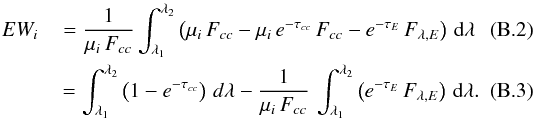$\begin{array}{ccc}\mathit{E}{\mathit{W}}_{\mathit{i}}& \mathrm{=}\frac{\mathrm{1}}{{\mathit{\mu }}_{\mathit{i}}\hspace{0.17em}{\mathit{F}}_{\mathit{cc}}}{\mathrm{\int }}_{{\mathit{\lambda }}_{\mathrm{1}}}^{{\mathit{\lambda }}_{\mathrm{2}}}\left({\mathit{\mu }}_{\mathit{i}}\hspace{0.17em}{\mathit{F}}_{\mathit{cc}}\mathrm{-}{\mathit{\mu }}_{\mathit{i}}\hspace{0.17em}{\mathit{e}}^{\mathrm{-}{\mathit{\tau }}_{\mathit{cc}}}\hspace{0.17em}{\mathit{F}}_{\mathit{cc}}\mathrm{-}{\mathit{e}}^{\mathrm{-}{\mathit{\tau }}_{\mathit{E}}}\hspace{0.17em}{\mathit{F}}_{\mathit{\lambda ,E}}\right)\hspace{0.17em}\mathrm{d}\mathit{\lambda }& \\ & \hspace{0.17em}\mathrm{=}{\mathrm{\int }}_{{\mathit{\lambda }}_{\mathrm{1}}}^{{\mathit{\lambda }}_{\mathrm{2}}}\left(\mathrm{1}\mathrm{-}{\mathit{e}}^{\mathrm{-}{\mathit{\tau }}_{\mathit{cc}}}\right)\hspace{0.17em}\mathit{d\lambda }\mathrm{-}\frac{\mathrm{1}}{{\mathit{\mu }}_{\mathit{i}}\hspace{0.17em}{\mathit{F}}_{\mathit{cc}}}\hspace{0.17em}{\mathrm{\int }}_{{\mathit{\lambda }}_{\mathrm{1}}}^{{\mathit{\lambda }}_{\mathrm{2}}}\left({\mathit{e}}^{\mathrm{-}{\mathit{\tau }}_{\mathit{E}}}\hspace{0.17em}{\mathit{F}}_{\mathit{\lambda ,E}}\right)\hspace{0.17em}\mathrm{d}\mathit{\lambda }\mathit{.}& \end{array}$The difference of equivalent width, ΔEW = EW_D − EW_A, can be derived from the above equation specialized for the pair of images, i.e., 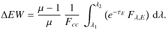$\begin{array}{ccc}\mathrm{\Delta }\mathit{EW}\mathrm{=}\frac{\mathit{\mu }\mathrm{-}\mathrm{1}}{\mathit{\mu }}\hspace{0.17em}\frac{\mathrm{1}}{{\mathit{F}}_{\mathit{cc}}}\hspace{0.17em}{\mathrm{\int }}_{{\mathit{\lambda }}_{\mathrm{1}}}^{{\mathit{\lambda }}_{\mathrm{2}}}\left({\mathit{e}}^{\mathrm{-}{\mathit{\tau }}_{\mathit{E}}}\hspace{0.17em}{\mathit{F}}_{\mathit{\lambda ,E}}\right)\hspace{0.17em}\mathrm{d}\mathit{\lambda }\mathit{.}& & \end{array}$(B.4)It results from this equation that when μ > 1, one may only observe EW_D > EW_A.

Appendix B.2: Compact + extended continua

We now consider that there is no flux from the emission line (F_λ,E = 0) over the wavelength range [λ₁,λ₂], but two sources of continuum: a compact continuum microlensed by a factor μ_i and an extended continuum F_ce which is not microlensed. Assuming that the continuum flux is constant over the range [λ₁,λ₂] such that F_λ,cc = F_cc and F_λ,ce = F_ce, we obtain $\begin{array}{ccc}\mathit{E}{\mathit{W}}_{\mathit{i}}\mathrm{=}\hspace{0.17em}& \frac{\mathrm{1}}{{\mathrm{ℱ}}_{\mathit{i}}}\hspace{0.17em}{\mathrm{\int }}_{{\mathit{\lambda }}_{\mathrm{1}}}^{{\mathit{\lambda }}_{\mathrm{2}}}\left({\mathit{\mu }}_{\mathit{i}}\hspace{0.17em}{\mathit{F}}_{\mathit{cc}}\mathrm{+}{\mathit{F}}_{\mathit{ce}}\mathrm{-}{\mathit{\mu }}_{\mathit{i}}\hspace{0.17em}{\mathit{e}}^{\mathrm{-}{\mathit{\tau }}_{\mathit{cc}}}\hspace{0.17em}{\mathit{F}}_{\mathit{cc}}\mathrm{-}{\mathit{e}}^{\mathrm{-}{\mathit{\tau }}_{\mathit{ce}}}\hspace{0.17em}{\mathit{F}}_{\mathit{ce}}\right)\hspace{0.17em}\mathrm{d}\mathit{\lambda } & \\ \mathrm{=}\hspace{0.17em}& \frac{\mathrm{1}}{{\mathrm{ℱ}}_{\mathit{i}}}{\mathrm{\int }}_{{\mathit{\lambda }}_{\mathrm{1}}}^{{\mathit{\lambda }}_{\mathrm{2}}}\left[{\mathit{\mu }}_{\mathit{i}}\hspace{0.17em}{\mathit{F}}_{\mathit{cc}}\left(\mathrm{1}\mathrm{-}{\mathit{e}}^{\mathrm{-}{\mathit{\tau }}_{\mathit{cc}}}\right)\mathrm{+}\left({\mathit{e}}^{\mathrm{-}{\mathit{\tau }}_{\mathit{ce}}}\hspace{0.17em}{\mathit{F}}_{\mathit{ce}}\right)\right]\hspace{0.17em}\mathrm{d}\mathit{\lambda ,}& \end{array}$where we defined ℱ_i = μ_iF_cc + F_ce, the flux in the unabsorbed continuum.

The difference of equivalent width ΔEW = EW_D − EW_A, is then 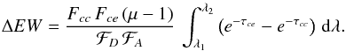$\begin{array}{ccc}\mathrm{\Delta }\mathit{EW}\mathrm{=}\frac{{\mathit{F}}_{\mathit{cc}}\hspace{0.17em}{\mathit{F}}_{\mathit{ce}}\hspace{0.17em}\mathrm{(}\mathit{\mu }\mathrm{-}\mathrm{1}\mathrm{)}}{{\mathrm{ℱ}}_{\mathit{D}}\hspace{0.17em}{\mathrm{ℱ}}_{\mathit{A}}}\hspace{0.17em}{\mathrm{\int }}_{{\mathit{\lambda }}_{\mathrm{1}}}^{{\mathit{\lambda }}_{\mathrm{2}}}\left({\mathit{e}}^{\mathrm{-}{\mathit{\tau }}_{\mathit{ce}}}\mathrm{-}{\mathit{e}}^{\mathrm{-}{\mathit{\tau }}_{\mathit{cc}}}\right)\hspace{0.17em}\mathrm{d}\mathit{\lambda }\mathit{.}& & \end{array}$(B.7)We clearly see that a difference of equivalent width is only detected if there is a difference of opacity between the absorbers covering the extended and the compact continua, i.e., τ_cc ≠ τ_ce. If μ > 1, we find ΔEW > 0 (EW_D > EW_A), and if τ_cc > τ_ce, and conversely ΔEW < 0 (EW_A > EW_D) if τ_cc<τ_ce.

Appendix B.3: Compact + extended continua + emission line

The situation where the source of light under the absorption is the sum of a compact and an extended continuum and of an emission line, directly results from the two previous cases. If we define the flux of the unabsorbed continuum of image A and D, ℱ_A = F_cc + F_ce, and ℱ_D = μF_cc + F_ce, then we can write the following difference of equivalent width ΔEW = EW_D − EW_A between images D and A:$\begin{array}{ccc}\mathrm{\Delta }\mathit{EW}\mathrm{=}\frac{{\mathit{F}}_{\mathit{cc}}\hspace{0.17em}\mathrm{(}\mathit{\mu }\mathrm{-}\mathrm{1}\mathrm{)}}{{\mathrm{ℱ}}_{\mathit{D}}\hspace{0.17em}{\mathrm{ℱ}}_{\mathit{A}}}{\mathrm{\int }}_{{\mathit{\lambda }}_{\mathrm{1}}}^{{\mathit{\lambda }}_{\mathrm{2}}}\left[{\mathit{F}}_{\mathit{ce}}\hspace{0.17em}\left({\mathit{e}}^{\mathrm{-}{\mathit{\tau }}_{\mathit{ce}}}\mathrm{-}{\mathit{e}}^{\mathrm{-}{\mathit{\tau }}_{\mathit{cc}}}\right)\mathrm{+}{\mathit{e}}^{\mathrm{-}{\mathit{\tau }}_{\mathit{E}}}\hspace{0.17em}{\mathit{F}}_{\mathit{\lambda ,E}}\right]\hspace{0.17em}\mathrm{d}\mathit{\lambda }\mathit{.}& & \end{array}$(B.8)

From this equation, we see that when μ > 1 and τ_cc > τ_ce (i.e., when the compact continuum is more absorbed than the extended continuum), ΔEW > 0. Conversely, ΔEW < 0 can only be obtained if τ_cc<τ_ce, i.e., when the compact continuum is less absorbed than the extended continuum. Positive value of ΔEW may also occur depending on the absorption rate of the different components, and on the relative contribution of the extended continuum and of the emission line.

Acknowledgments

We are very grateful to Joachim Wambsganss for making available his inverse ray-shooting code used for simulating the microlensing maps of H1413+117. We thank Ari Laor for enlightening discussions, and the referee for useful comments which helped to improve the presentation of our results. D.S. acknowledges support from a Back to Belgium grant from the Belgian Federal Science Policy (BELSPO), and partial funding from the Deutsche Forschungsgemeinschaft, reference SL172/1-1. D.H. and L.B. are respectively Senior Research Associate and Research Assistant at the F.R.S.-FNRS. Support for T. Anguita is provided by the Ministry of Economy, Development, and Tourism’s Millennium Science Initiative through grant IC120009, awarded to The Millennium Institute of Astrophysics, MAS and proyecto FONDECYT 11130630. This work was supported by the Fonds de la Recherche Scientifique – FNRS under grant 4.4501.05. This research made use of Astropy, a community-developed core Python package for Astronomy (The Astropy Collaboration 2013).

References

All Tables

All Figures

Fig. 1 Spectra of images A (black) and D (red) in the spectral range 1300–1700 Å, covering the Si iv-C iv  lines. The left and middle panels show the spectra as observed in 1989, 1993, 2000, and 2011, after normalization to unity in the continuum. The three shaded areas correspond to regions where the absorption changed significantly over the past 20 years, as discussed in Sect. 3.2. The top and bottom right panels show the change of intrinsic absorption over time for images A and D.

In the text

Fig. 2 MmD performed on images A and D of H1413+117 in 2011, using M = 0.4 (Sect. 3.3). The dashed blue line is the flux of image A. The thick black line is the fraction of the flux FM unaffected by microlensing for μ = 2.0. The red line is the corresponding microlensed fraction of the flux FMμ (shifted up to ease legibility), the dotted horizontal line is the line corresponding to FMμ = 0. The gray lines show the decomposition for two other values of μ (see Sect. 3.2). The three shaded areas correspond to the three regions A1 − A3 as discussed in the text.

In the text

	Fig. 3 Time variation of the equivalent width of the absorption, in the wavelength ranges A1–A3 (see legend), for image A (solid) and D (dashed).
In the text

	Fig. 4 MmD for Ly α +N v (top left), C iii] (top right), H β (bottom left), H α (bottom right) emissions. The values of A = M × μ derived for each line are based on the individual frames, while the MmD is shown for the sum of the individual spectra.
In the text

Fig. 5 Probability distribution for the size of the disc R1/2, and for the power-law index ν of the temperature profile. Solid contours correspond to the constraints obtained after correction of the microlensing amplitude for the presence of an extended continuum, and the dashed contours show the constraints if we do not account for the extended continuum. Contours are 68.3, 95.5, and 99.7% confidence level. The corresponding peaks of the probability distribution are shown as a filled black star and red cross, respectively.

In the text

Fig. 6 PDF of the source size for a standard accretion disc model (ν = 4/3) and various fractions of compact objects f∗ (extreme values f∗ = 1, shown in light gray, and f∗ = 0.01, shown in dark gray, correspond to 100% and 1% of the total matter being compact, respectively). The thick blue line is the result obtained assuming the same prior on f∗, as in Fig. 5, namely the prior resulting from the analysis of Pooley et al. (2012). The vertical solid line is the theory size for a Shakura-Sunyaev model based on Eq. (10) for cos(i) = 0.5 (R1/2 ~ 3.04 × 1015 cm ~10-3 pc).

In the text

References

- Angonin, M.-C., Vanderriest, C., Remy, M., & Surdej, J. 1990, A&A, 233, L5 [NASA ADS] [Google Scholar]
- Anguita, T., Schmidt, R. W., Turner, E. L., et al. 2008, A&A, 480, 327 [NASA ADS] [CrossRef] [EDP Sciences] [Google Scholar]
- Arav, N., Borguet, B., Chamberlain, C., Edmonds, D., & Danforth, C. 2013, MNRAS, 436, 3286 [NASA ADS] [CrossRef] [Google Scholar]
- Bate, N. F., Floyd, D. J. E., Webster, R. L., & Wyithe, J. S. B. 2008, MNRAS, 391, 1955 [NASA ADS] [CrossRef] [Google Scholar]
- Blackburne, J. A., Pooley, D., Rappaport, S., & Schechter, P. L. 2011, ApJ, 729, 34 [NASA ADS] [CrossRef] [Google Scholar]
- Borguet, B., & Hutsemékers, D. 2010, A&A, 515, A22 [NASA ADS] [CrossRef] [EDP Sciences] [Google Scholar]
- Borguet, B., Hutsemékers, D., Letawe, G., Letawe, Y., & Magain, P. 2008, A&A, 478, 321 [NASA ADS] [CrossRef] [EDP Sciences] [Google Scholar]
- Braibant, L., Hutsemékers, D., Sluse, D., Anguita, T., & García-Vergara, C. J. 2014, A&A, 565, L11 [NASA ADS] [CrossRef] [EDP Sciences] [Google Scholar]
- Capellupo, D. M., Hamann, F., Shields, J. C., Halpern, J. P., & Barlow, T. A. 2013, MNRAS, 429 [Google Scholar]
- Capellupo, D. M., Hamann, F., & Barlow, T. A. 2014, MNRAS, 444, 1893 [NASA ADS] [CrossRef] [Google Scholar]
- Chae, K.-H., Turnshek, D. A., Schulte-Ladbeck, R. E., Rao, S. M., & Lupie, O. L. 2001, ApJ, 561, 653 [NASA ADS] [CrossRef] [Google Scholar]
- Chartas, G., Eracleous, M., Dai, X., Agol, E., & Gallagher, S. 2007, ApJ, 661, 678 [NASA ADS] [CrossRef] [Google Scholar]
- Dai, X., Kochanek, C. S., Chartas, G., et al. 2010, ApJ, 709, 278 [NASA ADS] [CrossRef] [Google Scholar]
- Davis, S. W., & Laor, A. 2011, ApJ, 728, 98 [CrossRef] [Google Scholar]
- Eigenbrod, A., Courbin, F., Meylan, G., et al. 2008, A&A, 490, 933 [NASA ADS] [CrossRef] [EDP Sciences] [Google Scholar]
- Filiz Ak, N., Brandt, W. N., Hall, P. B., et al. 2012, ApJ, 757, 114 [NASA ADS] [CrossRef] [Google Scholar]
- Floyd, D. J. E., Bate, N. F., & Webster, R. L. 2009, MNRAS, 398, 233 [NASA ADS] [CrossRef] [Google Scholar]
- Goicoechea, L. J., & Shalyapin, V. N. 2010, ApJ, 708, 995 [NASA ADS] [CrossRef] [Google Scholar]
- Grier, C. J., Hall, P. B., Brandt, W. N., et al. 2015, ApJ, 806, 111 [NASA ADS] [CrossRef] [Google Scholar]
- Hall, P. B., Noordeh, E. S., Chajet, L. S., Weiss, E., & Nixon, C. J. 2014, MNRAS, 442, 1090 [NASA ADS] [CrossRef] [Google Scholar]
- Hutsemékers, D. 1993, A&A, 280, 435 [NASA ADS] [Google Scholar]
- Hutsemékers, D., Borguet, B., Sluse, D., Riaud, P., & Anguita, T. 2010, A&A, 519, A103 [NASA ADS] [CrossRef] [EDP Sciences] [Google Scholar]
- Jiménez-Vicente, J., Mediavilla, E., Muñoz, J. A., & Kochanek, C. S. 2012, ApJ, 751, 106 [NASA ADS] [CrossRef] [Google Scholar]
- Jiménez-Vicente, J., Mediavilla, E., Kochanek, C. S., & Muñoz, J. A. 2015, ApJ, 799, 149 [NASA ADS] [CrossRef] [Google Scholar]
- Kneib, J.-P., Alloin, D., & Pello, R. 1998, A&A, 339, L65 [NASA ADS] [Google Scholar]
- Kochanek, C. S. 2004, ApJ, 605, 58 [Google Scholar]
- Lamy, H., & Hutsemékers, D. 2004, A&A, 427, 107 [NASA ADS] [CrossRef] [EDP Sciences] [Google Scholar]
- Laor, A., & Davis, S. W. 2014, MNRAS, 438, 3024 [NASA ADS] [CrossRef] [Google Scholar]
- Lawrence, A. 2012, MNRAS, 423, 451 [NASA ADS] [CrossRef] [Google Scholar]
- Lewis, G. F., & Irwin, M. J. 1996, MNRAS, 283, 225 [NASA ADS] [Google Scholar]
- Lundgren, B. F., Wilhite, B. C., Brunner, R. J., et al. 2007, ApJ, 656, 73 [NASA ADS] [CrossRef] [Google Scholar]
- MacLeod, C. L., Kochanek, C. S., & Agol, E. 2009, ApJ, 699, 1578 [NASA ADS] [CrossRef] [Google Scholar]
- Magain, P., Surdej, J., Swings, J.-P., Borgeest, U., & Kayser, R. 1988, Nature, 334, 325 [NASA ADS] [CrossRef] [Google Scholar]
- Monier, E. M., Turnshek, D. A., & Lupie, O. L. 1998, ApJ, 496, 177 [NASA ADS] [CrossRef] [Google Scholar]
- Morgan, C. W., Kochanek, C. S., .Morgan, N. D., & Falco, E. E. 2010, ApJ, 712, 1129 [NASA ADS] [CrossRef] [Google Scholar]
- Mortonson, M. J., Schechter, P. L., & Wambsganss, J. 2005, ApJ, 628, 594 [NASA ADS] [CrossRef] [Google Scholar]
- Mosquera, A. M., & Kochanek, C. S. 2011, ApJ, 738, 96 [NASA ADS] [CrossRef] [Google Scholar]
- Muñoz, J. A., Mediavilla, E., Kochanek, C. S., Falco, E., & Mosquera, A. M. 2011, ApJ, 742, 67 [NASA ADS] [CrossRef] [Google Scholar]
- O’Dowd, M. J., Bate, N. F., Webster, R. L., Labrie, K., & Rogers, J. 2015, ArXiv e-prints [arXiv:1504.07160] [Google Scholar]
- Østensen, R., Remy, M., Lindblad, P. O., et al. 1997, A&AS, 126, 393 [NASA ADS] [CrossRef] [EDP Sciences] [Google Scholar]
- Poindexter, S., & Kochanek, C. S. 2010, ApJ, 712, 658 [NASA ADS] [CrossRef] [Google Scholar]
- Pooley, D., Rappaport, S., Blackburne, J. A., Schechter, P. L., & Wambsganss, J. 2012, ApJ, 744, 111 [NASA ADS] [CrossRef] [Google Scholar]
- Rathna Kumar, S., Stalin, C. S., & Prabhu, T. P. 2015, A&A, 580, A38 [NASA ADS] [CrossRef] [EDP Sciences] [Google Scholar]
- Schmidt, G. D., & Hines, D. C. 1999, ApJ, 512, 125 [NASA ADS] [CrossRef] [Google Scholar]
- Shakura, N. I., & Sunyaev, R. A. 1973, A&A, 24, 337 [NASA ADS] [Google Scholar]
- Sluse, D., Claeskens, J.-F., Hutsemékers, D., & Surdej, J. 2007, A&A, 468, 885 [NASA ADS] [CrossRef] [EDP Sciences] [Google Scholar]
- Sluse, D., Chantry, V., Magain, P., Courbin, F., & Meylan, G. 2012a, A&A, 538, A99 [NASA ADS] [CrossRef] [EDP Sciences] [Google Scholar]
- Sluse, D., Hutsemékers, D., Courbin, F., Meylan, G., & Wambsganss, J. 2012b, A&A, 544, A62 [NASA ADS] [CrossRef] [EDP Sciences] [Google Scholar]
- Smette, A., Surdej, J., Shaver, P. A., et al. 1992, ApJ, 389, 39 [NASA ADS] [CrossRef] [Google Scholar]
- The Astropy Collaboration, Robitaille, T. P., Tollerud, E. J., et al. 2013, A&A, 558, A33 [NASA ADS] [CrossRef] [EDP Sciences] [Google Scholar]
- Wambsganss, J. 1998, Living Rev. Relativity, 1, 12 [NASA ADS] [CrossRef] [Google Scholar]
- Wildy, C., & Goad, M. R. 2015, MNRAS, 448, 2397 [NASA ADS] [CrossRef] [Google Scholar]
- Zakamska, N. L., Strauss, M. A., Krolik, J. H., et al. 2006, AJ, 132, 1496 [NASA ADS] [CrossRef] [Google Scholar]