| Issue |
A&A
Volume 582, October 2015
|
|
|---|---|---|
| Article Number | A35 | |
| Number of page(s) | 14 | |
| Section | Extragalactic astronomy | |
| DOI | https://doi.org/10.1051/0004-6361/201526311 | |
| Published online | 01 October 2015 | |
Oxygen abundance distributions in six late-type galaxies based on SALT spectra of H II regions⋆
1 Astronomisches Rechen-Institut, Zentrum für Astronomie der Universität Heidelberg, Mönchhofstr. 12–14, 69120 Heidelberg, Germany
e-mail: This email address is being protected from spambots. You need JavaScript enabled to view it.
2 Main Astronomical Observatory, National Academy of Sciences of Ukraine, 27 Akademika Zabolotnoho St., 03680 Kyiv, Ukraine
3 South African Astronomical Observatory, PO Box 9, 7935 Observatory, Cape Town, South Africa
4 Southern African Large Telescope Foundation, PO Box 9, 7935 Observatory, Cape Town, South Africa
5 Sternberg Astronomical Institute, Lomonosov Moscow State University, Universitetskij Pr. 13, 119992 Moscow, Russia
6 Kazan Federal University, 18 Kremlyovskaya St., 420008 Kazan, Russian Federation
Received: 14 April 2015
Accepted: 4 August 2015
Abstract
Spectra of 34 H ii regions in the late-type galaxies NGC 1087, NGC 2967, NGC 3023, NGC 4030, NGC 4123, and NGC 4517A were observed with the South African Large Telescope (SALT). In all 34 H ii regions, oxygen abundances were determined through the “counterpart” method (C method). Additionally, in two H ii regions in which we detected auroral lines, we measured oxygen abundances with the classic Te method. We also estimated the abundances in our H ii regions using the O3N2 and N2 calibrations and compared those with the C-based abundances. With these data, we examined the radial abundance distributions in the disks of our target galaxies. We derived surface-brightness profiles and other characteristics of the disks (the surface brightness at the disk center and the disk scale length) in three photometric bands for each galaxy using publicly available photometric imaging data. The radial distributions of the oxygen abundances predicted by the relation between abundance and disk surface brightness in the W1 band obtained for spiral galaxies in our previous study are close to the radial distributions of the oxygen abundances determined from the analysis of the emission line spectra for four galaxies where this relation is applicable. Hence, when the surface-brightness profile of a late-type galaxy is known, this parametric relation can be used to estimate the likely present-day oxygen abundance in the disk of the galaxy.
Key words: galaxies: abundances / HII regions / galaxies: general
Based on observations made with the Southern African Large Telescope, programs 2012-1-RSA_OTH-001, 2012-2-RSA_OTH-003 and 2013-1-RSA_OTH-005.
© ESO, 2015
1. Introduction
Metallicities play a key role in studies of galaxies. The present-day abundance distributions across a galaxy provide important information about the evolutionary status of that galaxy and form the basis for the construction of models of the chemical evolution of galaxies.
Oxygen abundances and their gradients in the disks of late-type galaxies are typically based on emission-line spectra of individual H ii regions. When the auroral line [O iii]λ4363 is detected in the spectrum of an H ii region, the Te-based oxygen (O/H)Te abundance can be derived using the standard equations of the Te-method. In our current study, we do not always have this information and use alternative methods where the auroral line is not detected. In those cases, we estimate the oxygen abundances from strong emission lines using a recently suggested method (called the “C method”) for abundance determinations of Pilyugin et al. (2012) and Pilyugin et al. (2014a). When the strong lines R3, N2, and S2 are measured in the spectrum of an H ii region, the oxygen (O/H)CSN abundance can be determined. When the strong lines R2, R3, and N2 are measured in the spectrum, we can measure the oxygen (O/H)CON abundance.
It should be emphasized that the C method produces abundances on the same metallicity scale as the Te-method. In contrast, metallicities derived using one of the many calibrations based on photoionization models tend to show large discrepancies (of up to ~0.6 dex) with respect to Te-based abundances (see the reviews by Kewley & Ellison 2008; López-Sánchez & Esteban 2010; López-Sánchez et al. 2012). Coupling our emission-line measurements with available line measurements from the literature or public databases, we measured the radial distributions of the oxygen abundances across the disks of six galaxies.
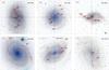 |
Fig. 1 SDSS images of our target galaxies with marked positions of the slits used in the present investigation. |
The study of the correlations between the oxygen abundance and other properties of spiral and irregular galaxies is important for understanding the formation and evolution of galaxies. The correlation between the local oxygen abundance and the stellar surface brightness (the OH – SB relation) or surface mass density has been a subject of discussion for a long time (Webster & Smith 1983; Edmunds & Pagel 1984; Vila-Costas & Edmunds 1992; Ryder 1995; Moran et al. 2012; Rosales-Ortega et al. 2012; Sánchez et al. 2014). We examined the relations between the oxygen abundance and the disk surface brightness in the infrared W1 band of the Wide-field Infrared Survey Explorer (WISE; Wright et al. 2010) at different fractions of the optical isophotal radius R25 in our previous paper (Pilyugin et al. 2014b). We found evidence that the OH – SB relation depends on the galactocentric distance taken as a fraction of the optical radius R25 and on other properties of a galaxy, namely its disk scale length and the morphological T-type. In that study, we suggested a parametric OH – SB relation for spiral galaxies.
In our current paper, we present results from observations of emission-line spectra of H ii regions in six spiral galaxies. These observations were obtained with the South African Large Telescope as a part of our investigation of the abundance properties of nearby late-type galaxies (Pilyugin et al. 2014a,b).
We constructed radial surface-brightness profiles of our galaxies in the infrared W1 band using the photometric maps obtained by the WISE satellite (Wright et al. 2010). The characteristics of the disk for each galaxy were obtained through bulge-disk decomposition. The radial distributions of the oxygen abundances predicted by the parametric OH – SB relation are compared to the radial distributions of the oxygen abundances determined from the analysis of the emission-line spectra of the H ii regions in our target galaxies.
Adopted and derived properties of our target galaxies.
The paper is organized as follows. Our sample of galaxies is presented in Sect. 2. The spectroscopic observations and data reduction are described in Sect. 3. The photometric properties of our galaxies are discussed in Sect. 4. The oxygen abundances are presented in Sect. 5. Section 6 contains a discussion and a brief summary of the main results.
Throughout the paper, we use the following standard notations for the line intensities I: R = I[ O III ] λ4363/IHβ, R2 = I[ O II ] λ3727 + λ3729/IHβ, N2 = I[ N II ] λ6548 + λ6584/IHβ, S2 = I[ S II ] λ6717 + λ6731/IHβ, R3 = I[ O III ] λ4959 + λ5007/IHβ.
2. Our galaxy sample
Our original sample of spiral galaxies for follow-up observations with the Southern African Large Telescope (SALT; Buckley et al. 2006; O’Donoghue et al. 2006) was devised based on Sloan Digital Sky Survey (SDSS) images and the fact that SALT can observe targets with a declination δ< 10 degrees and has a field of view of 8 arcmin. Each selected spiral galaxy contains a sufficiently large number of bright H ii regions distributed across the whole galaxy disk and fitting SALT’s field of view. The total sample consists of ~30 nearby galaxies that are located in the equatorial sky region.
Out of this sample of 58 galaxies, we have obtained spectra of H ii regions in six galaxies (NGC 1087, NGC 2967, NGC 3023, NGC 4030, NGC 4123, NGC 4517A) thus far. In Fig. 1 we present the images and slit positions for those galaxies. For a detailed description of the observations, we refer to Sect. 3.
Table 1 lists the general characteristics of each galaxy. We listed the most widely used identifications for our target galaxies, i.e., the designations in the New General Catalogue (NGC) and in the Uppsala General Catalog of Galaxies (UGC). The morphological type of the galaxy and morphological type code T were adopted from leda (Lyon-Meudon Extragalactic Database; Paturel et al. 1989, 2003). The right ascension and declination were taken from the NASA/IPAC Extragalactic Database (ned)1. The inclination of each galaxy, the position angle of the major axis, and the isophotal radius R25 in arcmin of each galaxy were determined in our current study. The distances were taken from ned. These distances include flow corrections for the Virgo cluster, the Great Attractor, and Shapley Supercluster infall. The isophotal radius in kpc was estimated from the isophotal radius R25 in arcmin and the distance listed above. The characteristics of the disks (the surface brightness at the disk center in the W1 band and the disk scale length) were determined through the bulge-disk decomposition carried out in our current paper. The surface brightness at the disk center was reduced to a face-on galaxy orientation and is given in terms of L⊙ pc-2.
Three galaxies of our sample are members of pairs of galaxies and are included in the “Catalogue of Isolated Pairs of Galaxies in the Northern Hemisphere” (Karachentsev 1972): NGC 3023 = KPG 216B, NGC 4123 = KPG 322B, NGC 4517A = KPG 344A. Two galaxies of our sample, NGC 2967 and NGC 4030, are known members of galaxy groups (Fouqué et al. 1992; Garcia 1993). The galaxy NGC 4517A is a low surface brightness galaxy (Romanishin et al. 1983).
3. Spectroscopic observations and reduction
3.1. Observing procedures
The spectroscopic observations of our selected galaxies were obtained with the multiobject spectroscopic mode (MOS) of the Robert Stobie Spectrograph (RSS; Burgh et al. 2003; Kobulnicky et al. 2003) installed at SALT. For each galaxy from our sample, we constructed a MOS mask, where the slit positions for the H ii regions were selected using gri SDSS images. A typical MOS mask thus devised contained 9–12 slits for H ii regions distributed over the whole galaxy disk. The usual width of the slits was 1.5 arcsec. The general strategy of the observations was to cover the total spectral range of 3600–7000 Å in order to detect: (1) the Balmer lines Hδ, Hγ, Hβ and Hα, which were used for extinction corrections; and (2) various emission lines used for the calculation of abundances: [O ii] λ3727, 3729, [O iii] λ4363, [O iii] λ4959, 5007, [N ii] λ6548, 6584, and [S ii] λ6717, 6731. We chose a resolution of R = 1000–2000 to be able to resolve emission lines located close to each other, e.g., Hγ and [O iii] λ4363, or [S ii] λ6717, and [S ii] λ6731.
In the MOS mode, the actual spectral coverage for each slit varies slightly depending on the X-position of a given slit relative to the center of the mask. Thus, to cover the total desired spectral range of 3600–7000 Å for each slit of the mask we had to obtain two spectral setups for each studied galaxy. One setup ranges from 3500–6500 Å, referred to as the blue setup hereafter, and one setup is from 5000–7000 Å, called the red setup hereafter; we combined these setups after reducing the data. The volume phase holographic (VPH) grating GR900 was used to cover the blue setup with a final reciprocal dispersion of ~0.97 Å pixel-1 and a spectral resolution resulting in a FWHM of 5–6 Å (R ~ 1000). To cover the red setup, we used the VPH grating GR1300 with a final reciprocal dispersion of ~0.64 Å pixel-1 and a spectral resolution with a FWHM of 3–4 Å (R ~ 1600). All observations were carried out between June 2012 and April 2013.
During an observation at the SALT telescope the mirror remains at a fixed altitude and azimuth and the image of an astronomical target produced by the telescope is followed by the “tracker”, which is located at the position of the prime focus (similar in operation to the Arecibo Radio Telescope). This results in only a limited observing window per target. For this reason each observation consisted usually of two exposures of about 1000 s each to fit a single SALT visibility track. For the same reason the blue and red setups were usually observed on different nights.
Spectra of Ar comparison arcs and a set of quartz tungsten halogen flats were obtained immediately after each observation to calibrate the wavelength scale and to correct for pixel-to-pixel variations. A set of spectrophotometric standard stars was observed during twilight time for the relative flux calibration. Since SALT has a variable pupil size, an absolute flux calibration is not possible even using spectrophotometric standard stars. All details of the observations are summarized in Table 2. In total, 34 H ii regions in six galaxies were observed.
The primary reduction of the SALT data was done with the SALT science pipeline (Crawford et al. 2010). After that, the bias- and gain-corrected and mosaicked MOS data were reduced in the way described below.
Journal of the observations.
3.2. Data reduction and line flux measurements
Cosmic ray rejection was done using the IRAF2 task lacose_spec (van Dokkum 2001). The wavelength calibration was accomplished using the IRAF tasks identify, reidentify, fitcoord, and transform. The spectral data were divided by the illumination-corrected flat field to correct for pixel-to-pixel sensitivity variations of the detector. After that two-dimensional spectra were extracted from the MOS images for each slit. The background subtraction was done using the IRAF task background. Since we used a multislit mask, the slits for the individual objects have a length of ~5−20 arcsec and the background was fitted by a low-order polynomial function along the spatial slit coordinate at each wavelength. This allows us to extract the flux from the H ii regions only, without galactic stellar background. The spectra were corrected for sensitivity effects using the Sutherland extinction curve and a sensitivity curve obtained from observed standard star spectra. Finally, all two-dimensional spectra of a slit position obtained with the same observational setup were averaged.
From each two-dimensional spectrum of the blue and red setups, one-dimensional spectra were extracted in spatial direction for each pixel along the slit. We refer to these spectra as “one-pixel-wide”. The line fluxes ([O ii]λλ3727,3729, [O iii]λ4363, Hβ, [O iii]λ4959, [O iii]λ5007, [N ii]λ6548, Hα, [N ii]λ6584, [S ii]λ6717, and [S ii]λ6731) were then measured with IRAF or/and by fitting the lines with Gaussians following Pilyugin & Thuan (2007) and Pilyugin et al. (2010a).
We first consider the distribution of the emission-line fluxes along the slit. The measured fluxes in the Hβ and R3 emission lines in the blue and red one-pixel-wide spectra for slit 8 in NGC 3023 as a function of the pixel number along the slit are shown in Fig. 2. Examination of Fig. 2 shows that the position of the peak in the Hβ (and R3) emission line in the red spectrum is shifted as compared to that in the blue spectrum by approximately three pixels. This shows that the position of the slit of the red spectrum does not coincide with the position of the slit for the blue spectrum. Instead they are shifted in the direction along the slit by approximately three pixels with respect to each other. Inspection of Fig. 2 also shows that the form of the distribution of the Hβ (and R3) emission-line flux per pixel in the red spectrum differs from that in the blue spectrum. This demonstrates that the position of the slit for the red spectrum is also shifted in the direction perpendicular to the slit or that the position angles of the red and blue spectrum are different. This prevents us from considering the lines of the blue and red spectra together. Therefore we derived the abundances using the lines from the blue (or red) spectrum individually.
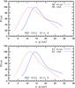 |
Fig. 2 Fluxes in the Hβ (upper panel) and R3 (lower panel) emission lines in the blue (solid lines) and red (dashed lines) spectra as a function of the pixel number along the slit for slit 8 in NGC 3023. The fluxes are in arbitrary units. |
The full set of lines [O ii]λλ3727, 3729, Hβ, [O iii]λ5007, Hα, and [N ii]λ6548 or Hβ, [O iii]λ5007, Hα, [N ii]λ6584, and [S ii]λλ6717, 6731 is needed to correct for interstellar reddening and to determine the oxygen abundances. For this reason, only slits that provide at least one of these line sets in either the blue or red setup are chosen for further study. As the actual spectral coverage for each of our slits varies slightly depending on the position of a given slit on the mask, in some cases the Hβ+[O iii]λ5007 lines of the red spectra and the Hα+[N ii]λ6548 lines of the blue spectra are shifted beyond the actual spectral coverage of the slit. This is the reason why the number of the presented observations of H ii regions varies from one in NGC 4030 to up to nine in NGC 1087.
We constructed the aperture for the blue and red spectra by averaging the seven one-pixel-wide spectra near the flux maximum. As mentioned before, the emission from the underlying stellar population of the galactic disk was subtracted during the background correction, i.e., we removed the stellar continuum averaged along the spatial slit coordinates near the H ii region. Since the continuum in the spectra of our H ii regions is sufficiently weak or undetectable, we neglected possible stellar absorption by the stellar populations of the H ii regions. The measured emission fluxes F were corrected for interstellar reddening. We obtained the extinction coefficient C(Hβ) using the theoretical Hα-to-Hβ ratio (=2.878) and the analytical approximation to the Whitford interstellar reddening law of Izotov et al. (1994).
Dereddened emission line fluxes in units of the Hβ line flux and the extinction coefficient C(Hβ) in the blue spectra of a sample of the target H ii regions in NGC 3023.
Dereddened emission line fluxes in units of the Hβ line flux and the extinction coefficient C(Hβ) in the red spectra of a sample of the target H ii regions in our galaxy sample.
The dereddened emission-line fluxes in the averaged spectra of the target H ii regions are listed in Table 3 for the blue spectra and in Table 4 for the red spectra. The theoretical ratio of [N ii]λ6584/[N ii]λ6548 is constant and close to 3 (Storey & Zeippen 2000) since those lines originate from transitions from the same energy level. Since the [N ii]λ6584 line measurements are more reliable than the [N ii]λ6548 line measurements, the value of N2 is estimated as N2 = 1.33 × [N ii]λ6584 unless indicated otherwise. Similarly, the value of R3 can be estimated as R3 = 1.33 × [O iii]λ5007 since the [O iii]λ5007 and [O iii]λ4959 lines also originate from transitions from the same energy level and their flux ratio is very close to 3 (Storey & Zeippen 2000; Kniazev et al. 2004). Therefore, the [N ii]λ6548 and λ4959 lines are not included in Tables 3 and 4.
The uncertainty of the emission-line flux εline is estimated taking the uncertainty of the continuum level, errors in the line flux, and the uncertainty in the sensitivity curve into account (see Kniazev et al. 2004, for details). The uncertainty of the continuum, εcont, is determined in the region near the emission line where the continuum is approximated by a linear fit. The line-flux uncertainty, εflux, is estimated as the deviation from a Gaussian profile. The uncertainty in the sensitivity curve, εsc, is less than 2−3% in all considered wavelength ranges (see, e.g., Kniazev 2012). We adopt the maximum value of the relative uncertainty as εsc = 0.03.
4. Photometry
To estimate the deprojected galactocentric distance (normalized to the optical isophotal radius R25) of the H ii region from its coordinates on the celestial sphere, one needs to know the values of the inclination, i, the position angle of the major axis, PA, and the isophotal radius of a galaxy, R25. It is common practice to take those values from de Vaucouleurs et al. (1991, thereafter RC3) or from the leda database. However, some values from those sources show a significant difference for galaxies from our list. For example, the isophotal radius of NGC 4517A in the RC3 is larger by a factor of two than that given in the leda database. Therefore we obtained our own estimates of the values of i, PA, and R25 for our target galaxies.
We analyzed the publicly available photometric maps in the infrared W1 band with an isophotal wavelength of 3.4 μm obtained by the (WISE; Wright et al. 2010) and in the g and r bands obtained by the SDSS data release (DR) 9 (Ahn et al. 2012). We derived the surface-brightness profile and disk orientation parameters in three photometric bands for each galaxy. The determinations of the surface-brightness profile, position angle, and ellipticity were performed for each band separately in the way described in Pilyugin et al. (2014b). For NGC 3023, however, we were not able to estimate reliable values of the position angle and ellipticity for the g and r bands. Therefore, for this galaxy the values of the position angle and ellipticity obtained for the W1 band were used for the construction of the surface-brightness profiles in all three filters.
It should be noted that the WISE and SDSS surveys are sufficiently deep for our surface-brightness profiles to extend beyond the optical isophotal radii R25. The obtained surface-brightness profiles are shown in Fig. 3. The adopted inclinations and position angles are given in Table 1.
The value of the isophotal radius is derived from the obtained surface-brightness profiles in the g and r bands. Surface-brightness measurements were corrected for foreground Galactic extinction using the AV values from the recalibration by Schlafly & Finkbeiner (2011) of the extinction maps of Schlegel et al. (1998) and the extinction curve of Cardelli et al. (1989), assuming a ratio of total to selective extinction of RV = AV/EB − V = 3.1. We adopted the AV values given in the NASA Extragalactic Database ned. Afterward, we corrected the surface-brightness measurements for the inclination. The measurements in the SDSS filters g and r were converted to B-band magnitudes, and the AB magnitudes were reduced to the Vega photometric system using the conversion relations and solar magnitudes of Blanton & Roweis (2007). First, we obtained the B-band magnitudes from the g and r magnitudes ![Mathematical equation: \begin{equation} B_{\rm AB} = g + 0.2354 + 0.3915\;[(g-r)-0.6102] , \label{equation:bgr} \end{equation}](/articles/aa/full_html/2015/10/aa26311-15/aa26311-15-eq59.png) (1)where the BAB, g, and r magnitudes in Eq. (1) are in the AB photometric system. Then, the AB magnitudes were reduced to the Vega photometric system
(1)where the BAB, g, and r magnitudes in Eq. (1) are in the AB photometric system. Then, the AB magnitudes were reduced to the Vega photometric system 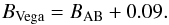 (2)The obtained isophotal radii are given in Table 1.
 |
Fig. 3 Observed surface-brightness profiles of our galaxies in the g and r bands of the SDSS photometric system and in the W1 band of the WISE photometric system. The X-axis shows the galactocentric radius in arcsec and the Y-axis the surface brightness in mag arcsec-2. The optical isophotal radius R25 is marked with an arrow. |
 |
Fig. 4 Comparison between the measured surface-brightness profiles of NGC 4123 in the B band reported by Weiner et al. (2001; solid line), by Micheva et al. (2013; long dashed line), and obtained here (short dashed line). The X-axis shows the galactocentric radius in arcmin, and the Y-axis the surface brightness in mag arcsec-2. The arrow indicates the optical isophotal radius R25. |
 |
Fig. 5 Patterns resulting from the bulge-disk decomposition of our target galaxies (X-axis: galactocentric radius in kpc, Y-axis: logarithm of the central surface brightness for a face-on galaxy orientation in solar luminosities per pc2). Each panel shows the decomposition assuming a purely exponential profile for the disk. The measured surface profile is plotted using gray (blue) circles. The bulge contribution is shown with a dotted line, the disk contribution with a dashed line, and the total (bulge + disk) fit with a solid line. |
Surface brightness profiles of the galaxy NGC 4123 in the B band were published by Weiner et al. (2001) and Micheva et al. (2013). Figure 4 shows the comparison between their profiles with that derived here from the photometric imaging data in the SDSS g and r bands.
We performed a bulge-disk decomposition of the observed surface-brightness profiles using a purely exponential disk (PED) approximation in the same way as in Pilyugin et al. (2014b). Exponential profiles were used to fit the observed disk surface-brightness profiles, and the bulge profiles were fitted with a general Sérsic profile. The observed surface-brightness profiles of five galaxies from our sample are fitted satisfactorily well. The upper panel of Fig. 5 shows the bulge-disk decomposition of the galaxy NGC 1087 as an example. The measured surface profile is marked by circles. The fit to the bulge contribution is shown with a dotted line, the fit to the disk with a dashed line, and the total (bulge + disk) fitting with a solid line. Table 1 lists the parameters of the disk surface-brightness profiles of those galaxies in the W1 band: the logarithm of the central surface brightness of the disk in the W1 band reduced to a face-on galaxy orientation in terms of L⊙ pc-2 and the disk scale length in the W1 band, hW1 in kpc. Those values are parameters of the exponential disk approximation, described in detail in Pilyugin et al. (2014b).
For the galaxy NGC 3023, we could not determine a reliable disk scale length, hW1, and central surface brightness of the disk, (ΣLW1)0. The lower panel of Fig. 5 shows the surface-brightness-profile fit for this galaxy. The disk contribution to the surface brightness is close to the observed surface-brightness profile over a small interval of radial distances only (in fact, this is a bulge-dominated galaxy). Therefore, the values of the disk scale length and central surface brightness of the disk are questionable.
 |
Fig. 6 Diagram of [N ii]λ6584/Hα versus [O iii]λ5007/Hβ . The symbols denote results for the measured H ii regions in our target galaxies. The solid line separates objects with H ii region spectra from those containing an AGN according to Kauffmann et al. (2003), while the dashed line represents the same separation according to the work by Kewley et al. (2001). The gray (light blue) filled circles show a large sample of emission-line SDSS galaxies from Thuan et al. (2010). |
5. Abundances
5.1. Abundance determination
Baldwin et al. (1981) proposed the [OIII]λ5007/Hβ vs. [NII]λ6584/Hα diagram (the so-called BPT classification diagram), which is often used to distinguish between star-forming regions and active galactic nuclei (AGNs). The exact location of the dividing line between star-forming regions and AGNs is still controversial (see, e.g., Kewley et al. 2001; Kauffmann et al. 2003). Figure 6 shows the positions of our targets (open circles) in the BPT classification diagram. The solid line is the dividing line between star-forming regions and AGNs according to Kauffmann et al. (2003), while the dashed line is the same line according to Kewley et al. (2001). Regardless of which line is adopted, Fig. 6 shows that all our objects are H ii regions and their oxygen abundances can be estimated using standard techniques.
The Te-based oxygen (O/H)Te abundances of the H ii regions with the detected auroral line [O iii]λ4363 were determined using the equations for the Te-method from Pilyugin et al. (2010b, 2012).
A new method (called the “C method”) for oxygen and nitrogen abundance determinations from strong emission lines was recently suggested (Pilyugin et al. 2012, 2014a). In our red spectra, we measured the strong lines R3, N2, and S2, which allowed us to determine the oxygen (O/H)CNS abundances using those strong lines. In some of our blue spectra, the strong lines R2, R3, and N2 were measured and applied to determine the oxygen (O/H)CON abundances.
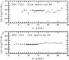 |
Fig. 7 Oxygen abundances along the slit for the slit 8 in the NGC 3023. The circles in the upper panel show the oxygen abundances determined from the individual blue one-pixel-width spectra through the Te method. The solid line is the abundance obtained from the integrated seven-pixel-width spectrum through the Te method. The circles in the lower panel show the oxygen abundances determined from the individual red one-pixel-width spectra through the CNS method. The solid line is the abundance obtained from the integrated seven-pixel-width spectrum through the CNS method. |
5.2. The robustness and precision of the abundance determination
The emission-line fluxes measured in the one-pixel-wide spectra represent the radiation of a small part of the H ii region. One would expect that the Te-based abundances in a given H ii region derived from the spectra of different areas on the H ii region image should be the same or at least should be close to each other. Is this the case for the abundances estimated from the counterpart method? To clarify this matter we have estimated the oxygen abundances from the individual one-pixel-wide spectra and considered the variations in those abundances.
Figure 7 shows the distribution of the oxygen abundances along the slit for the bright, extend H ii region (#8) in NGC 3023, i.e., the abundance estimated from the individual one-pixel-wide spectra as a function of the number of the pixel along the slit. The auroral line R = [O iii]λ4363 is detected in around 20 individual one-pixel-wide spectra of this H ii region. The circles in the upper panel of the Fig. 7 show the oxygen abundances determined from the individual blue one-pixel-wide spectra through the Te method. The solid line is the Te-based abundance obtained from the seven-pixel-wide spectrum. The circles in the lower panel of the Fig. 7 show the oxygen abundances determined from the individual red one-pixel-wide spectra through the CNS method. The solid line represents the abundance obtained from the seven-pixel-width spectrum through the CNS method.
Inspection of the upper panel of Fig. 7 confirms that the Te-based abundances are independent from the position in the H ii region image at which the measurement was taken. Examination of the lower panel of Fig. 7 shows that the abundances determined from the individual one-pixel-wide spectra through the C method are close to each other and are close to the abundance obtained from the integrated seven-pixel-wide spectrum. A similar picture was found for other H ii regions. Thus, the C-based abundances are robust and independent from the specific area covered by the measurement in an H ii region image, i.e., the C method produces a reliable oxygen abundance even if a spectrum of only part of an H ii region is used.
The scatter in individual C-based abundances is even lower than the scatter in individual Te-based abundances, i.e., the formal uncertainty in the C-based abundances is lower than that in the Te-based abundances. This can be attributed to the fact that the measurements of the weak auroral lines used in the Te method can involve larger errors than the measurements of the strong lines used in the C method. It should be noted, however, that the true uncertainty in the C-based oxygen abundance depends on the accuracy of the strong-line measurements in the spectrum of the target H ii region as well as on the reliability of the abundance determinations in the reference H ii regions. Our current sample of reference H ii regions (our standard reference sample from 2013) contains 250 H ii regions for which the absolute differences in the oxygen abundances (O/H)CON – (O/H)Te and (O/H)CNS – (O/H)Te and in the nitrogen abundances (N/H)CON – (N/H)Te and (N/H)CNS – (N/H)Te are less than 0.1 dex (Pilyugin et al. 2014a). Thus the true uncertainty in the C-based oxygen abundance may be up to around 0.1 dex even if the formal error due to the uncertainties in the strong line measurement is small. Therefore we assume that the uncertainties in the obtained oxygen abundances in our investigated H ii regions in the current paper can exceed 0.1 dex, although the formal error caused by the uncertainty in the line fluxes measurement is lower.
5.3. Radial gradients
The radial distribution of the oxygen abundances across the disk within the isophotal radius in each of our target galaxies was fitted with the following equation:  (3)where 12 + log(O/H)R0 is the oxygen abundance at R0 = 0, i.e., the extrapolated central oxygen abundance, CO/H, is the slope of the oxygen abundance gradient expressed in terms of dex
  , and R/R25 is the fractional radius, i.e., the galactocentric distance normalized to the disk’s isophotal radius R25.
NGC 1087. The strong lines Hβ, [O iii]λλ4959, 5007, Hα, [N ii]λλ6548, 6584, and [S ii]λλ6717, 6731 were measured in nine red spectra. In those H ii regions, we derived the oxygen abundance (O/H)CNS. The resulting oxygen abundances are listed in Table 5. Those abundances are shown by the filled circles in panel a of Fig. 8.
There are three SDSS spectra of H ii regions in the galaxy NGC 1087 in data release 7 (DR7, Abazajian et al. 2009), namely Sp 409-51871-237, Sp 1069-52590-193, and Sp 1511-52946-192. (The SDSS spectrum number consists of the SDSS plate number, the modified Julian date of the observation, and the number of the fiber on the plate.) Since SDSS data release 10 (DR10, Ahn et al. 2014) reported line measurements in only one spectrum, we used the SDSS spectra from DR7. The oxygen (O/H)CNS abundances inferred using the SDSS spectra are shown with open (blue) circles in panel a) of Fig. 8.
Oxygen abundances in the H ii regions in the disks of our sample of galaxies.
The best linear fit to all the data points (12 points) with galactocentric distances smaller than the isophotal R25 radius is  (4)with a mean deviation of 0.034 dex around the relationship. The obtained relation is shown by a solid line in panel a) of Fig. 8.
NGC 2967. The strong lines Hβ, [O iii]λλ4959,5007, Hα, [N ii]λλ6548,6584 and [S ii]λλ6717,6731 were measured in six red spectra. Oxygen (O/H)CNS abundances were then inferred for those H ii regions. These abundances are shown with filled circles in panel b) of Fig. 8. The strong lines [O ii]λλ3727,3729, Hβ, [O iii]λλ4959,5007, Hα, and [N ii]λ6584 were measured in two blue spectra of H ii regions in the galaxy NGC 2967 and were used to estimate oxygen (O/H)CON abundances. Those abundances are shown with black filled squares in panel b) of Fig. 8. The obtained oxygen abundances are given in Table 5.
There are three SDSS spectra (Sp 476-52314-622, Sp 266-51630-387, and 266-51602-394) of H ii regions in the galaxy NGC 2967 in DR7. The oxygen (O/H)CNS abundances derived using the SDSS spectra are shown with gray (blue) open circles in panel b) of Fig. 8.
The best linear fit to all the data points (11 points) with galactocentric distances smaller the isophotal R25 radius is  (5)with a mean deviation of 0.026 dex around the relationship. The resulting relation is represented with a solid line in panel b) of Fig. 8.
NGC 3023. The auroral line R = [O iii]λ4363 was detected in two blue spectra of H ii regions in the disk of NGC 3023. The oxygen abundances in those H ii regions were determined through the direct Te method. Those abundances are shown with plus signs in panel c) of Fig. 8. The strong lines [O ii]λλ3727, 3729, Hβ, [O iii]λλ4959, 5007, Hα, and [N ii]λ6548 were measured in one blue spectrum. We derived the oxygen (O/H)CON abundance, finding the total nitrogen flux N2 to be 4 [N ii]λ6548. This abundance is shown with the black filled square in panel c of Fig. 8. The strong lines Hβ, [O iii]λλ4959, 5007, Hα, [N ii]λλ6548, 6584, and [S ii]λλ6717, 6731 were measured in seven red spectra and used to infer the oxygen (O/H)CNS abundance for those H ii regions. The total nitrogen fluxes were determined to be N2 = 1.33[N iiλ6584. Those abundances are shown with black filled circles in panel c) of Fig. 8.
 |
Fig. 8 Radial distributions of oxygen abundances in the disks of our target galaxies. The plus signs are abundances derived through the Te method, the circles are abundances obtained through the CNS method, and the squares are those inferred through the CON method. The filled symbols show abundances based on our SALT spectra, the open (blue) symbols are abundances based on spectra from the literature (see text). The solid line in each panel is the best linear fit to the data points with galactocentric distances less than the isophotal R25 radius. (A color version of this figure is available in the online version.) |
There are four SDSS spectra (Sp 480-51989-056, Sp 481-51908-289, Sp 267-51608-384, and Sp 267-51608-389) of H ii regions in the galaxy NGC 3023. Since there is a large discrepancy between the line fluxes reported in DR7 and DR10, these SDSS spectra were not used.
The best linear fit to the data points (nine points) with galactocentric distances smaller than the isophotal R25 radius is  (6)with a mean deviation of 0.047 dex around the relationship. The obtained relation is plotted with a solid line in panel c) of Fig. 8.
NGC 4030. Unfortunately, the spectral setup used for this galaxy only covers the wavelengths of the Hα and [N ii]λ6584 lines for one of the slits. Therefore, the strong lines [O ii]λλ3727,3729, Hβ, [O iii]λλ4959,5007, Hα, and [N ii]λ6584 were measured in only one blue spectrum of an H ii region in the galaxy NGC 4030. The oxygen (O/H)CON abundance was estimated using the measured strong lines. The inferred abundance is shown with black filled squares in panel d of Fig. 8. There are six SDSS spectra (Sp 285-51930-042, Sp 285-51663-044, Sp 285-51930-049, Sp 285-51663-058, Sp 331-52368-405, and Sp 2892-54552-293) of H ii regions in the galaxy NGC 4030 in DR7. The oxygen (O/H)CNS abundances based on the SDSS spectra are shown with gray (blue) open circles in panel d of Fig. 8.
The best linear fit to all the data points (seven points) with galactocentric distances smaller the isophotal R25 radius is  (7)with a mean deviation of 0.009 dex from the relationship. The relation is shown with a solid line in panel d) of Fig. 8.
NGC 4123. The strong lines [O ii]λλ3727,3729, Hβ, [O iii]λλ4959,5007, Hα, and [N ii]λ6584 were measured in five blue spectra of H ii regions in the galaxy NGC 4123. The oxygen (O/H)CON abundances based on those spectral data are shown with black filled squares in panel e) of Fig. 8. The sulfur lines [S ii]λλ6717,6731 were also measured in the blue spectrum of one H ii region in the galaxy NGC 4123. This allowed us to obtain the oxygen (O/H)CNS abundance for this particular H ii region. The strong lines Hβ, [O iii]λλ4959, 5007, Hα, [N ii]λλ6548, 6584, and [S ii]λλ6717, 6731 were measured in two red spectra. The inferred oxygen (O/H)CNS abundances are shown with the black filled circles in panel e) of Fig. 8. It should be noted that the H ii region at the center of NGC 4123 (Slit 06) is located close to the line dividing AGNs and star-forming regions in the BPT classification diagram.
Spectra of the region near the center of the NGC 4123 were observed by Kehrig et al. (2004) and by SDSS (Sp 517-52024-504). We obtained abundances of 12+log(O/H)CNS = 8.56 and 12+log(O/H)CON = 8.63 using the spectral measurements of Kehrig et al. (2004). Moreover, we measured an abundance of 12+log(O/H)CNS = 8.63 using the DR10 line fluxes.
The best linear fit to all the data points (ten points) with galactocentric distances smaller than the isophotal R25 radius is  (8)with a mean deviation of 0.025 dex. This relation is represented with a solid line in panel e) of Fig. 8.
 |
Fig. 9 Comparison of the radial distributions of oxygen abundances in the disks of our target galaxies determined through the C method (filled dark [black] circles), via the O3N2 calibration (open gray [red] circles), and through the N2 calibration (plus signs). The solid line in each panel is the best linear fit to the (O/H)C abundances (the same as in Fig. 8). (A color version of this figure is available in the online version.) |
NGC 4517A. The strong lines [O ii]λλ3727,3729, Hβ, [O iii]λλ4959, 5007, Hα, and [N ii]λ6584 were measured in the blue spectrum of an H ii region in the galaxy NGC 4517A. In another spectrum, the line [N ii]λ6584 is out of our spectral range, but the line [N ii]λ6548 is included. We derived the oxygen (O/H)CON abundance in these spectra. The total nitrogen flux N2 was determined to be N2 = 1.33[N ii]λ6584 in the former case and to be N2 = 4 [N ii]λ6548 in the latter case. These abundances are shown with black filled squares in panel f) of Fig. 8.
Romanishin et al. (1983) reported emission-line ratios [S ii](λ6717 + λ6731)/Hα, Hα/[N ii](λ6548 + λ6584), and [O iii](λ4959+λ5007)/Hβ obtained from photographic spectra of four H ii regions in NGC 4517A. We estimated the oxygen (O/H)CSN and nitrogen (N/H)CSN abundances from those strong lines. Romanishin et al. (1983) did not provide the positions of the observed H ii regions, but listed the deprojected radii instead. We corrected these galactocentric distances for the galaxy distance adopted here and used the resulting values. Furthermore, there are two SDSS spectra (Sp 289-51990-627 and Sp 290-51941-350) of H ii regions in NGC 4517A. The abundances based on the SDSS and Romanishin et al.’s data are shown with gray (blue) open circles in panel f) of Fig. 8.
The best linear fit to all the data points (eight points) with galactocentric distances smaller than the isophotal R25 radius is  (9)with a mean deviation of 0.023 dex. This relation is indicated by a solid line in panel f) of Fig. 8.
5.4. Comparison between the distributions of the abundances determined through the C method and via the O3N2 and N2 calibrations
Many calibrations based on photoionization models and/or H ii regions with abundances determined through the direct Te-method were suggested for nebular abundance determinations (Pagel et al. 1979; Alloin et al. 1979; Dopita & Evans 1986; McGaugh 1991; Zaritsky et al. 1994; Pilyugin 2000, 2001; Kewley & Dopita 2002; Pettini & Pagel 2004; Pilyugin & Thuan 2005; Tremonti et al. 2004; Stasińska 2006, among many others). The discrepancies between metallicities of a given H ii region derived using different calibrations can be large, up to ~0.6 dex (see reviews by Kewley & Ellison 2008; López-Sánchez & Esteban 2010; López-Sánchez et al. 2012). However, one would expect that all the calibrations based on the abundances in H ii regions determined through the Te method should produce the abundances close to each other. Since the C method produces abundances on the same metallicity scale as the Te-method, those abundances should be close to the abundances produced by other calibrations based on the direct abundances in H ii regions.
The O3N2 and N2 calibrations suggested by Pettini & Pagel (2004) are widely used. The original O3N2 and N2 calibrations are hybrid calibrations, i.e., they are based on both H ii regions with abundances determined through the direct Te-method and photoionization models. Pure empirical O3N2 and N2 calibrations, i.e., based on H ii regions with abundances determined through the direct Te-method, were recently presented by Marino et al. (2013). Thus we determined the (O/H)O3N2 abundances in our H ii regions also using the O3N2 calibration of Marino et al. (2013), i.e.,  (10)where O3N2 = log[([ O III ] λ5007 / Hβ)/[ N II ] λ6584 / Hα) ], and the (O/H)N2 abundances using their N2 calibration
  (11)where N2 = log([ N II ] λ6584 / Hα).
Figure 9 shows the comparison of the radial distributions of the oxygen abundances in the disks of our target galaxies determined through the C method (filled dark [black] circles), via the O3N2 calibration (open gray [red] circles), and through the N2 calibration (plus signs). The solid line in each panel is the best linear fit to the (O/H)C abundances (the same as in Fig. 8).
 |
Fig. 10 Comparison of the oxygen abundances in the individual H ii regions of our sample determined through the C method with oxygen abundances obtained through the O3N2 calibration (upper panel) and through the N2 calibration (lower panel). The solid line indicates a one-to-one correspondence. The dashed lines are shifted by ± 0.1 dex. |
Figure 10 shows the comparison of the oxygen abundances in the individual H ii regions of our sample determined through the C method with the oxygen abundances obtained through the O3N2 calibration (upper panel) and through the N2 calibration (lower panel).
Figures 9 and 10 demonstrate that the (O/H)O3N2 abundances are in satisfactory agreement (within 0.1 dex) with the (O/H)C abundances for H ii regions with metallicities 12+log(O/H) ≳ 8.1. However, a small systematic difference, around 0.05 dex, between (O/H)O3N2 and (O/H)C abundances seems to exist; in the sense that the (O/H)O3N2 abundances are slightly lower than the (O/H)C abundances. A large disagreement between (O/H)O3N2 and (O/H)C abundances for H ii regions with metallicities 12+log(O/H)C≲ 8.1 is not surprising since the O3N2 calibration of Marino et al. (2013) is constructed for H ii regions with metallicities 12+log(O/H) ≳ 8.1 and does not work at low metallicities. The differences between the (O/H)N2 and (O/H)C abundances exceed 0.1 dex for some H ii regions with metallicities 12+log(O/H) ≳ 8.1. This may suggest that the O3N2 calibration of Marino et al. (2013) provides more reliable abundances than their N2 calibration.
In summary, the comparison between C-, O3N2-, and N2-based abundances in our target H ii regions allows us to suggest that the uncertainties in the obtained (O/H)C abundances are within ~0.1 dex. This supports our estimation of the uncertainties in the abundances discussed in Sect. 5.2.
6. Discussion
The radial distributions of the oxygen abundances across the disks of all the galaxies of our sample are well fitted by linear relationships within the isophotal radius (with the abundances on the logarithmic scale). The mean deviation from the relationship is less than 0.05 dex for each galaxy. The values of the radial abundance gradient vary by a factor of ~4 among the galaxies of our sample; from − 0.164 dex  for NGC 4123 to − 0.663 dex for NGC 4517A.
The correlation between the local oxygen abundance and the stellar surface brightness (OH – SB relation) or surface mass density has been discussed in many studies (Webster & Smith 1983; Edmunds & Pagel 1984; Vila-Costas & Edmunds 1992; Ryder 1995; Moran et al. 2012; Rosales-Ortega et al. 2012; Sánchez et al. 2014). In our previous paper (Pilyugin et al. 2014b), we examined the relations between the oxygen abundance and the disk surface brightness in the infrared W1 band of WISE at different fractions of the optical isophotal radius R25. We found evidence that the OH – SB relation varies with galactocentric distance and depends on the disk scale length and the morphological T-type of a galaxy. We derived a general parametric relation between abundance and surface brightness in the W1 band, O/H = f(SB) for spiral galaxies of type Sa – Sd,  (12)where x = r/R25 is the fractional radius expressed in terms of the isophotal radius of a galaxy (R25), (ΣL)x is the disk surface brightness, hW1 the radial disk scale length, and T the morphological T-type. It is interesting to compare the radial distributions of oxygen abundances predicted by this relationship to the radial abundance trends traced by the oxygen abundances in the H ii regions in the disks of our sample of galaxies.
 |
Fig. 11 Radial distributions of oxygen abundances in the disks of the spiral galaxies of our sample. The circles represent the abundances of the individual H ii regions (the same as in Fig. 8). The line in each panel shows the abundance distribution predicted by the relation between abundance and surface brightness in the W1 band, Eq. (12). |
Figure 11 shows the comparison between the radial distributions of the oxygen abundances predicted by the O/H = f(SB) relation, Eq. (12), and the abundances obtained from the analysis of the emission-line spectra of H ii regions for four of our galaxies, NGC 1087, NGC 2967, NGC 4030, and NGC 4123. The O/H = f(SB) relation cannot be applied to the other two galaxies of our sample. It was noted above that we could not determine a reliable disk scale length hW1 and surface brightness at the center of the disk of the galaxy NGC 3023 since the disk contribution to the surface brightness is close to the observed surface-brightness profile over a small range of radial distances only (see lower panel of Fig. 5). NGC 4517A is a Sdm galaxy (with morphological type T = 8), whereas the O/H = f(SB) relation was derived for spiral galaxies of the types Sa – Sd (i.e., for a range of morphological types from T ~ 1 to T ~ 7).
Inspection of Fig. 11 shows that the oxygen abundances predicted by the parametric O/H = f(SB) relation are rather close to the abundances obtained from the analysis of the emission-line spectra of H ii regions of the galaxies of the present sample where the OH – SB relation is applicable. The discrepancy usually does not exceed 0.1 dex. Thus, the parametric O/H = f(SB) relation can be used for a rough estimation of the oxygen abundances in the disks of spiral galaxies.
Summary
Spectra of H ii regions in six late-type galaxies were observed with the South African Large Telescope (SALT). The auroral line [O iii]λ4363 was detected in two spectra. The Te-based oxygen (O/H)Te abundances in these two H ii regions were derived using the equations of the standard Te-method. The oxygen abundances of the other H ii regions were estimated from strong emission lines through the recently suggested “counterpart” method (C method). When the strong lines R3, N2, and S2 were measured in our spectra, oxygen (O/H)CNS abundances could be obtained. When, on the other hand, the strong lines R2, R3, and N2 were available, then oxygen (O/H)CON abundances were determined. Moreover, we also inferred oxygen abundances of the H ii regions in our target galaxies with available spectral measurements from the literature or from the SDSS spectroscopic data base through the C method.
We derived oxygen abundances from the individual one-pixel-wide spectra and considered the variations in those abundances. The abundances determined with the C method from the individual one-pixel-wide spectra are close to each other and are close to the abundances obtained from the integrated seven-pixel-wide spectrum. This can be considered as supporting evidence for the robustness and precision of the C-based abundances, which are independent of the area in the H ii region image that is measured. In other words, the C method produces a reliable oxygen abundance even if a spectrum of only a part of an H ii region is used.
We also determined the (O/H)O3N2 and (O/H)N2 abundances in our target H ii regions using the O3N2 and N2 calibrations of Marino et al. (2013). The (O/H)O3N2 abundances are in satisfactory agreement (within 0.1 dex) with the (O/H)C abundances for H ii regions with metallicities 12+log(O/H) ≳ 8.1. However, a small systematic difference, around 0.05 dex, between (O/H)O3N2 and (O/H)C abundances seems to exist in the sense that the (O/H)O3N2 abundances are slightly lower than the (O/H)C abundances. The differences between the (O/H)N2 and (O/H)C abundances are larger than 0.1 dex for some H ii regions. This may suggest that the O3N2 calibration of Marino et al. (2013) provides more reliable abundances than their N2 calibration.
We determined the abundance gradients in the disks of our six late-type target galaxies. The radial distributions of the oxygen abundances across the disks of all the galaxies of our sample are well fitted by linear relationships within the isophotal radius (with abundances on a logarithmic scale). The mean deviation from the relationship is less than 0.05 dex for each galaxy. The values of the radial abundance gradient vary by a factor of ~4 among the galaxies of our sample, i.e., from − 0.164 dex for NGC 4123 to − 0.663 dex for NGC 4517A.
We derived surface-brightness profiles in three photometric bands (the W1 band of WISE and the g and r bands of the SDSS) for each galaxy using publicly available photometric imaging data. The characteristics of the disks (the surface brightness at the disk center and the disk scale length) were found through bulge-disk decomposition. Using the photometric parameters of the disks, the oxygen abundance distributions were estimated from the relation between abundance and surface brightness of the disk in the W1 band, O/H = SB, which had been obtained for spiral galaxies in our previous study. The oxygen abundances predicted by the O/H = SB relation are rather close to the bundances determined from the analysis of the emission-line spectra of the H ii regions in the galaxies of the present asample where the OH – SB relation is applicable. The discrepancy is usually not larger than 0.1 dex. Thus, the parametric O/H = f(SB) relation can be used for a rough estimation of the oxygen abundances in the disks of spiral galaxies.
The NASA/IPAC Extragalactic Database (ned) is operated by the Jet Populsion Laboratory, California Institute of Technology, under contract with the National Aeronautics and Space Administration. http://ned.ipac.caltech.edu/
IRAF is distributed by the National Optical Astronomical Observatories, which are operated by the Association of Universities for Research in Astronomy, Inc., under cooperative agreement with the National Science Foundation.
Acknowledgments
The observations reported in this paper were obtained with the Southern African Large Telescope (SALT). L.S.P., I.A.Z., and E.K.G. acknowledge support within the framework of Sonderforschungsbereich (SFB 881) on “The Milky Way System” (especially subproject A5), which is funded by the German Research Foundation (DFG). L.S.P. and I.A.Z. thank the Astronomisches Rechen-Institut at the Universität Heidelberg, where this investigation was carried out, for their hospitality. A.Y.K. acknowledges support from the National Research Foundation (NRF) of South Africa. This work was partly funded by the subsidy allocated to the Kazan Federal University for the state assignment in the sphere of scientific activities (L.S.P.). The authors acknowledge the work of the SDSS collaboration. Funding for SDSS-III has been provided by the Alfred P. Sloan Foundation, the Participating Institutions, the National Science Foundation, and the US Department of Energy Office of Science. The SDSS-III web site is http://www.sdss3.org/. SDSS-III is managed by the Astrophysical Research Consortium for the Participating Institutions of the SDSS-III Collaboration including the University of Arizona, the Brazilian Participation Group, Brookhaven National Laboratory, University of Cambridge, Carnegie Mellon University, University of Florida, the French Participation Group, the German Participation Group, Harvard University, the Instituto de Astrofisica de Canarias, the Michigan State/Notre Dame/JINA Participation Group, Johns Hopkins University, Lawrence Berkeley National Laboratory, Max Planck Institute for Astrophysics, Max Planck Institute for Extraterrestrial Physics, New Mexico State University, New York University, Ohio State University, Pennsylvania State University, University of Portsmouth, Princeton University, the Spanish Participation Group, University of Tokyo, University of Utah, Vanderbilt University, University of Virginia, University of Washington, and Yale University. We acknowledge the usage of the HyperLeda database (http://leda.univ-lyon1.fr).
References
- Abazajian, K. N., Adelman-McCarthy, J. K., Agüeros, M. A., et al. 2009, ApJS, 182, 543 [NASA ADS] [CrossRef] [Google Scholar]
- Ahn, C. P., Alexandroff, R., Allen de Prieto, C., et al. 2012, ApJS, 203, 21 [NASA ADS] [CrossRef] [Google Scholar]
- Ahn, C. P., Alexandroff, R., Allen de Prieto, C., et al. 2014, ApJS, 211, 17 [NASA ADS] [CrossRef] [Google Scholar]
- Alloin, D., Collin-Souffrin, S., Joly, M., & Vigroux, L. 1979, A&A, 78, 200 [Google Scholar]
- Baldwin, J. A., Phillips, M. M., & Terlevich, R. 1981, PASP, 93, 5 [NASA ADS] [CrossRef] [EDP Sciences] [Google Scholar]
- Blanton, M. R., & Roweis, S. 2007, AJ, 133, 734 [NASA ADS] [CrossRef] [Google Scholar]
- Buckley, D. A. H., Swart, G. P., & Meiring, J. G. 2006, SPIE, 6267 [Google Scholar]
- Burgh, E. B., Nordsieck, K. H., Kobulnicky, H. A., et al. 2003, SPIE, 4841, 1463 [Google Scholar]
- Cardelli, J. A., Clayton, G. C., & Mathis, J. S. 1989, ApJ, 345, 245 [NASA ADS] [CrossRef] [Google Scholar]
- Crawford, S. M., Still, M., Schellart, P., et al. 2010, SPIE, 7737, 54 [NASA ADS] [Google Scholar]
- de Vaucouleurs, G., de Vaucouleurs, A., Corwin, Jr., H. G., et al. 1991, Third Reference Catalogue of Bright Galaxies (Berlin, Heidelberg, New York: Springer-Verlag) [Google Scholar]
- Dopita, M. A., & Evans, I. N. 1986, ApJ, 307, 431 [NASA ADS] [CrossRef] [Google Scholar]
- Edmunds, M. G., & Pagel, B. E. J. 1984, MNRAS, 211, 507 [NASA ADS] [CrossRef] [Google Scholar]
- Fouqué, P., Gourgoulhon, E., Chamaraux, P., & Paturel, G. 1992, A&AS, 93, 211 [NASA ADS] [Google Scholar]
- Garcia, A. M. 1993, A&AS, 100, 47 [NASA ADS] [Google Scholar]
- Izotov, Y. I., Thuan, T. X., & Lipovetsky, V. A. 1994, ApJ, 435, 647 [NASA ADS] [CrossRef] [Google Scholar]
- Karachentsev, I. D. 1972, Soobshcheniya Spetsial’noj Astrofizicheskoj Observatorii, 7, 1 [Google Scholar]
- Kauffmann, G., Heckman, T. M., Tremonti, C., et al. 2003, MNRAS, 346, 1055 [Google Scholar]
- Kehrig, C., Telles, E., & Cuisinier, F. 2004, AJ, 128, 1141 [NASA ADS] [CrossRef] [Google Scholar]
- Kewley, L. J., & Dopita, M. A. 2002, ApJS, 142, 35 [NASA ADS] [CrossRef] [Google Scholar]
- Kewley, L. J., & Ellison, S. L. 2008, ApJ, 681, 1183 [NASA ADS] [CrossRef] [Google Scholar]
- Kewley, L. J., Dopita, M. A., Sutherland, R. S., Heisler, C. A., & Trevena, J. 2001, ApJ, 556, 121 [Google Scholar]
- Kniazev, A. Y. 2012, Astron. Lett., 38, 707 [NASA ADS] [CrossRef] [Google Scholar]
- Kniazev, A. Y., Pustilnik, S. A., Grebel, E. K., Lee, H., & Pramskij, A. G. 2004, ApJS, 153, 429 [NASA ADS] [CrossRef] [Google Scholar]
- Kobulnicky, H. A., Nordsieck, K. H., Burgh, E. B., et al. 2003, SPIE, 4841, 1634 [Google Scholar]
- López-Sánchez, Á. R., & Esteban, C. 2010, A&A, 517, A85 [NASA ADS] [CrossRef] [EDP Sciences] [Google Scholar]
- López-Sánchez, Á. R., Dopita, M. A., Kewley, L. J., et al. 2012, MNRAS, 426, 2630 [NASA ADS] [CrossRef] [Google Scholar]
- Marino, R. A., Rosales-Ortega, F. F., Sánchez, S. F., et al. 2013, A&A, 559, A114 [NASA ADS] [CrossRef] [EDP Sciences] [Google Scholar]
- McGaugh, S. S. 1991, ApJ, 380, 140 [NASA ADS] [CrossRef] [Google Scholar]
- Micheva, G., Östlin, G., Zackrisson, E., et al. 2013, A&A, 556, A10 [NASA ADS] [CrossRef] [EDP Sciences] [Google Scholar]
- Moran, S. M., Heckman, T. M., Kauffmann, G., et al. 2012, ApJ, 745, 66 [NASA ADS] [CrossRef] [Google Scholar]
- O’Donoghue, D., Buckley, D. A. H., Balona, L. A., et al. 2006, MNRAS, 372, 151 [NASA ADS] [CrossRef] [Google Scholar]
- Pagel, B. E. J., Edmunds, M. G., Blackwell, D. E., Chun, M. S., & Smith, G. 1979, MNRAS, 189, 95 [NASA ADS] [CrossRef] [Google Scholar]
- Paturel, G., Fouqué, P., Bottinelli, L., & Gouguenheim, L. 1989, A&AS, 80, 299 [NASA ADS] [Google Scholar]
- Paturel, G., Petit, C., Prugniel, P., et al. 2003, A&A, 412, 45 [NASA ADS] [CrossRef] [EDP Sciences] [Google Scholar]
- Pettini, M., & Pagel, B. E. J. 2004, MNRAS, 348, L59 [NASA ADS] [CrossRef] [Google Scholar]
- Pilyugin, L. S. 2000, A&A, 362, 325 [NASA ADS] [Google Scholar]
- Pilyugin, L. S. 2001, A&A, 369, 594 [NASA ADS] [CrossRef] [EDP Sciences] [Google Scholar]
- Pilyugin, L. S., & Thuan, T. X. 2005, ApJ, 631, 231 [NASA ADS] [CrossRef] [MathSciNet] [Google Scholar]
- Pilyugin, L. S., & Thuan, T. X. 2007, ApJ, 669, 299 [NASA ADS] [CrossRef] [Google Scholar]
- Pilyugin, L. S., Vílchez, J. M., Cedrés, B., & Thuan, T. X. 2010a, MNRAS, 403, 896 [NASA ADS] [CrossRef] [Google Scholar]
- Pilyugin, L. S., Vílchez, J. M., & Thuan, T. X. 2010b, ApJ, 720, 1738 [NASA ADS] [CrossRef] [Google Scholar]
- Pilyugin, L. S., Grebel, E. K., & Mattsson, L. 2012, MNRAS, 424, 2316 [NASA ADS] [CrossRef] [Google Scholar]
- Pilyugin, L. S., Grebel, E. K., & Kniazev, A. Y. 2014a, AJ, 147, 131 [NASA ADS] [CrossRef] [Google Scholar]
- Pilyugin, L. S., Grebel, E. K., Zinchenko, I. A., & Kniazev, A. Y. 2014b, AJ, 148, 134 [NASA ADS] [CrossRef] [Google Scholar]
- Romanishin, W., Strom, K. M., & Strom, S. E. 1983, ApJS, 53, 105 [NASA ADS] [CrossRef] [Google Scholar]
- Rosales-Ortega, F. F., Sánchez, S. F., Iglesias-Páramo, J., et al. 2012, ApJ, 756, L31 [NASA ADS] [CrossRef] [Google Scholar]
- Ryder, S. D. 1995, ApJ, 444, 610 [NASA ADS] [CrossRef] [Google Scholar]
- Sánchez, S. F., Rosales-Ortega, F. F., Iglesias-Páramo, J., et al. 2014, A&A, 563, A49 [NASA ADS] [CrossRef] [EDP Sciences] [Google Scholar]
- Schlafly, E. F., & Finkbeiner, D. P. 2011, ApJ, 737, 103 [NASA ADS] [CrossRef] [Google Scholar]
- Schlegel, D. J., Finkbeiner, D. P., & Davis, M. 1998, ApJ, 500, 525 [NASA ADS] [CrossRef] [Google Scholar]
- Stasińska, G. 2006, A&A, 454, L127 [NASA ADS] [CrossRef] [EDP Sciences] [Google Scholar]
- Storey, P. J., & Zeippen, C. J. 2000, MNRAS, 312, 813 [Google Scholar]
- Thuan, T. X., Pilyugin, L. S., & Zinchenko, I. A. 2010, ApJ, 712, 1029 [NASA ADS] [CrossRef] [Google Scholar]
- Tremonti, C. A., Heckman, T. M., Kauffmann, G., et al. 2004, ApJ, 613, 898 [NASA ADS] [CrossRef] [Google Scholar]
- van Dokkum, P. G. 2001, PASP, 113, 1420 [NASA ADS] [CrossRef] [Google Scholar]
- Vila-Costas, M. B., & Edmunds, M. G. 1992, MNRAS, 259, 121 [NASA ADS] [CrossRef] [Google Scholar]
- Webster, B. L., & Smith, M. G. 1983, MNRAS, 204, 743 [NASA ADS] [Google Scholar]
- Weiner, B. J., Williams, T. B., van Gorkom, J. H., & Sellwood, J. A. 2001, ApJ, 546, 916 [NASA ADS] [CrossRef] [Google Scholar]
- Wright, E. L., Eisenhardt, P. R. M., Mainzer, A. K., et al. 2010, AJ, 140, 1868 [NASA ADS] [CrossRef] [Google Scholar]
- Zaritsky, D., Kennicutt, Jr., R. C., & Huchra, J. P. 1994, ApJ, 420, 87 [NASA ADS] [CrossRef] [Google Scholar]
All Tables
Dereddened emission line fluxes in units of the Hβ line flux and the extinction coefficient C(Hβ) in the blue spectra of a sample of the target H ii regions in NGC 3023.
Dereddened emission line fluxes in units of the Hβ line flux and the extinction coefficient C(Hβ) in the red spectra of a sample of the target H ii regions in our galaxy sample.
All Figures
|
Fig. 1 SDSS images of our target galaxies with marked positions of the slits used in the present investigation. |
| In the text | |
|
Fig. 2 Fluxes in the Hβ (upper panel) and R3 (lower panel) emission lines in the blue (solid lines) and red (dashed lines) spectra as a function of the pixel number along the slit for slit 8 in NGC 3023. The fluxes are in arbitrary units. |
| In the text | |
|
Fig. 3 Observed surface-brightness profiles of our galaxies in the g and r bands of the SDSS photometric system and in the W1 band of the WISE photometric system. The X-axis shows the galactocentric radius in arcsec and the Y-axis the surface brightness in mag arcsec-2. The optical isophotal radius R25 is marked with an arrow. |
| In the text | |
|
Fig. 4 Comparison between the measured surface-brightness profiles of NGC 4123 in the B band reported by Weiner et al. (2001; solid line), by Micheva et al. (2013; long dashed line), and obtained here (short dashed line). The X-axis shows the galactocentric radius in arcmin, and the Y-axis the surface brightness in mag arcsec-2. The arrow indicates the optical isophotal radius R25. |
| In the text | |
|
Fig. 5 Patterns resulting from the bulge-disk decomposition of our target galaxies (X-axis: galactocentric radius in kpc, Y-axis: logarithm of the central surface brightness for a face-on galaxy orientation in solar luminosities per pc2). Each panel shows the decomposition assuming a purely exponential profile for the disk. The measured surface profile is plotted using gray (blue) circles. The bulge contribution is shown with a dotted line, the disk contribution with a dashed line, and the total (bulge + disk) fit with a solid line. |
| In the text | |
|
Fig. 6 Diagram of [N ii]λ6584/Hα versus [O iii]λ5007/Hβ . The symbols denote results for the measured H ii regions in our target galaxies. The solid line separates objects with H ii region spectra from those containing an AGN according to Kauffmann et al. (2003), while the dashed line represents the same separation according to the work by Kewley et al. (2001). The gray (light blue) filled circles show a large sample of emission-line SDSS galaxies from Thuan et al. (2010). |
| In the text | |
|
Fig. 7 Oxygen abundances along the slit for the slit 8 in the NGC 3023. The circles in the upper panel show the oxygen abundances determined from the individual blue one-pixel-width spectra through the Te method. The solid line is the abundance obtained from the integrated seven-pixel-width spectrum through the Te method. The circles in the lower panel show the oxygen abundances determined from the individual red one-pixel-width spectra through the CNS method. The solid line is the abundance obtained from the integrated seven-pixel-width spectrum through the CNS method. |
| In the text | |
|
Fig. 8 Radial distributions of oxygen abundances in the disks of our target galaxies. The plus signs are abundances derived through the Te method, the circles are abundances obtained through the CNS method, and the squares are those inferred through the CON method. The filled symbols show abundances based on our SALT spectra, the open (blue) symbols are abundances based on spectra from the literature (see text). The solid line in each panel is the best linear fit to the data points with galactocentric distances less than the isophotal R25 radius. (A color version of this figure is available in the online version.) |
| In the text | |
|
Fig. 9 Comparison of the radial distributions of oxygen abundances in the disks of our target galaxies determined through the C method (filled dark [black] circles), via the O3N2 calibration (open gray [red] circles), and through the N2 calibration (plus signs). The solid line in each panel is the best linear fit to the (O/H)C abundances (the same as in Fig. 8). (A color version of this figure is available in the online version.) |
| In the text | |
|
Fig. 10 Comparison of the oxygen abundances in the individual H ii regions of our sample determined through the C method with oxygen abundances obtained through the O3N2 calibration (upper panel) and through the N2 calibration (lower panel). The solid line indicates a one-to-one correspondence. The dashed lines are shifted by ± 0.1 dex. |
| In the text | |
|
Fig. 11 Radial distributions of oxygen abundances in the disks of the spiral galaxies of our sample. The circles represent the abundances of the individual H ii regions (the same as in Fig. 8). The line in each panel shows the abundance distribution predicted by the relation between abundance and surface brightness in the W1 band, Eq. (12). |
| In the text | |
Current usage metrics show cumulative count of Article Views (full-text article views including HTML views, PDF and ePub downloads, according to the available data) and Abstracts Views on Vision4Press platform.
Data correspond to usage on the plateform after 2015. The current usage metrics is available 48-96 hours after online publication and is updated daily on week days.
Initial download of the metrics may take a while.