| Issue |
A&A
Volume 582, October 2015
|
|
|---|---|---|
| Article Number | A87 | |
| Number of page(s) | 12 | |
| Section | Extragalactic astronomy | |
| DOI | https://doi.org/10.1051/0004-6361/201425209 | |
| Published online | 14 October 2015 | |
Suzaku X-ray study of the double radio relic galaxy cluster CIZA J2242.8+5301
1
SRON Netherlands Institute for Space Research, Sorbonnelaan 2, 3584 CA
Utrecht, The
Netherlands
e-mail: This email address is being protected from spambots. You need JavaScript enabled to view it.
2
Harvard-Smithsonian Center for Astrophysics,
60 Garden Street, Cambridge, MA
02138,
USA
3
Department of Earth and Planetary Science, The University of
Tokyo, 113-0033
Tokyo,
Japan
4
Leiden Observatory, Leiden University,
PO Box 9513, 2300 RA
Leiden, The
Netherlands
5
Hamburg Observatory, University of Hamburg,
Gojenbergsweg 112, 21029
Hamburg,
Germany
6
Thüringer Landessternwarte Tautenburg,
Sternwarte 5, 07778
Tautenburg,
Germany
7
Instituto de Astrofísica e Ciências do Espaço, Universidade de
Lisboa, OAL, Tapada da
Ajuda, 1349-018
Lisboa,
Portugal
8
Departamento de Física, Faculdade de Ciências, Universidade de
Lisboa, Edifício C8, Campo
Grande, 1749-016
Lisbon,
Portugal
Received:
23
October
2014
Accepted:
8
July
2015
Abstract
Context. We present the results from Suzaku observations of the merging cluster of galaxies CIZA J2242.8+5301 at z = 0.192.
Aims. To study the physics of gas heating and particle acceleration in cluster mergers, we investigated the X-ray emission from CIZA J2242.8+5301, which hosts two giant radio relics in the northern and southern part of the cluster.
Methods. We analyzed data from three-pointed Suzaku observations of CIZA J2242.8+5301 to derive the temperature distribution in four different directions.
Results. The intracluster medium (ICM) temperature shows a remarkable drop from 8.5-0.6+0.8 keV to 2.7-0.4+0.7 keV across the northern radio relic. The temperature drop is consistent with a Mach number ℳn = 2.7+0.7-0.4 and a shock velocity vshock:n = 2300-400+700 km s-1. We also confirm the temperature drop across the southern radio relic. However, the ICM temperature beyond this relic is much higher than beyond the northern relic, which gives a Mach number ℳs = 1.7+0.4-0.3 and shock velocity vshock:s = 2040-410+550 km s-1. These results agree with other systems showing a relationship between the radio relics and shock fronts which are induced by merging activity. We compare the X-ray derived Mach numbers with the radio derived Mach numbers from the radio spectral index under the assumption of diffusive shock acceleration in the linear test particle regime. For the northern radio relic, the Mach numbers derived from X-ray and radio observations agree with each other. Based on the shock velocities, we estimate that CIZA J2242.8+5301 is observed approximately 0.6 Gyr after core passage. The magnetic field pressure at the northern relic is estimated to be 9% of the thermal pressure.
Key words: shock waves / methods: data analysis / galaxies: clusters: individual: CIZA J2242.8+5301 / X-rays: galaxies: clusters / galaxies: clusters: intracluster medium
© ESO, 2015
1. Introduction
Based on the framework of the hierarchical structure formation theory, clusters of galaxies grow through merging events with smaller objects and accretion flows from large-scale structure filaments (Voit 2005; Kravtsov & Borgani 2012). In particular, merging events between massive clusters of galaxies are the most energetic events in the Universe since the Big Bang, releasing as much as ~1064 erg (Markevitch & Vikhlinin 2007). This gravitational energy is converted into the heating of the intracluster medium (ICM) and particle acceleration by shocks, likely via the mechanism of diffusive shock acceleration (DSA: Blandford & Eichler 1987).
Radio observations show the existence of diffuse nonthermal emission in clusters such as radio halos, relics and mini-halos (for a review, see Feretti et al. 2012; Brunetti & Jones 2014, and references therein). Among these radio structures, radio relics show remarkable features, such as a diffuse (Mpc-scale), elongated shape, and they are typically located at cluster outskirts. In addition, radio relics are usually seen in merging clusters. Therefore, radio relics are considered to be the result of synchrotron emission from relativistic electrons, which are accelerated by shocks induced by cluster mergers (Ensslin et al. 1998).
Because shocks play a fundamental role in cluster evolution, it is crucial to understand their properties (Mach number, shock velocity, shock acceleration efficiency, etc.). In particular, at high Mach numbers (ℳ ~ 103−104) DSA is known to have enough efficiency to accelerate particles from a thermal distribution to the high-energy regime. This is confirmed by observations of several supernova remnants (e.g., Koyama et al. 1995), however, shock fronts induced by cluster mergers are expected to have a much lower Mach number (ℳ ~ 2−5). The acceleration efficiency of these low-Mach number shocks is thought to be too low to reproduce the observed radio brightness (Kang et al. 2012). Recent work by Guo et al. (2014a,b), however, using detailed particle in cell simulations indicates that electron acceleration can be efficient at low-Mach number shocks in the ICM. More detailed studies of cluster shocks are highly desired for understanding their roles during merging activity.
Most evidence for shock fronts in clusters of galaxies is based on X-ray imaging studies (for a review, see Markevitch 2010, and references therein). Up to now, clear evidence for shock fronts are reported in 1E 0657-56 (Bullet cluster: Markevitch et al. 2002), A520 (Markevitch et al. 2005), A754 (Macario et al. 2011), A2146 (Russell et al. 2010, 2012), A521 (Bourdin et al. 2013), and A2034 (Owers et al. 2014).
Follow-up X-ray observations of the northwest radio relic in Abell 3667 revealed that the ICM temperature and surface brightness distribution drops across the relic, which indicates the existence of a shock front across the relic (Finoguenov et al. 2010). The correspondence between radio relics and shocks is also confirmed in other clusters (Macario et al. 2011; Akamatsu et al. 2012a,b, 2013; Ogrean & Brüggen 2013; Bourdin et al. 2013). Using the Rankine-Hugoniot jump conditions, the estimated Mach number from the temperature jump typically spans ℳ ~ 1.5−3.0 (Akamatsu & Kawahara 2013). These values are consistent with predictions from hydrodynamical simulations (Miniati et al. 2000; Ryu et al. 2003).
This paper reports the results of deep X-ray observations of the cluster CIZA J2242.8+5301 with Suzaku. It has been discovered in the Clusters in the Zone of Avoidance (CIZA) survey (z = 0.192: Kocevski et al. 2007). CIZA J2242.8+5301 has a clear double radio relic at a scale of several Mpc with a remarkably narrow width of 50 kpc for the northern relic (van Weeren et al. 2010). The relic is strongly polarized at the 50 to 60% level, indicating a well-ordered magnetic field, which is well aligned with the shock plane.
The northern relic shows an injection index at the edge of the relic of −0.6 ± 0.05 (van Weeren et al. 2010; Stroe et al. 2013), which corresponds to a Mach number of ℳ ~ 4.6. The spectral index for the south relic is also reported as −1.29 ± 0.05, which corresponds to a Mach number of ℳ ~ 2.8 (Stroe et al. 2013). Stroe et al. (2014b) also report the detection of radio emission at the high-frequency band (~16 GHz) and pose some questions for the diffusive shock acceleration predictions of the aging effect on relativistic electrons. A recent deep Chandra observation of CIZA J2242.8+5301 revealed several edges in the X-ray surface brightness distribution. Interestingly, the edges are found in the downstream regions of the shocks assumed to be associated with the radio relics, and have no counterpart in the temperature distribution (Ogrean et al. 2014).
Previous Suzaku observations of CIZA J2242.8+5301 showed a remarkable temperature jump from 8.3 keV to 2.1 keV across the northern relic (Akamatsu & Kawahara 2013). The Mach number estimated from the Rankine-Hugoniot condition is ℳX = 3.2 ± 0.5. On the other hand, as described above, van Weeren et al. (2010) reported a somewhat higher Mach number  . Similar higher values, ℳradio> ℳX, have been found for two other relics (1RXS J0603: van Weeren et al. 2012; Ogrean et al. 2013; Itahana et al. 2015). Recently, Sarazin et al. (2014) reported results of deep XMM-Newton observations of the northeast radio relic in Abell 3667. They derive a Mach number of 2.09 ± 0.09, which is clearly much smaller than the Mach number expected from the radio spectral index (spectrum index α = −0.6 ± 0.2, ℳ = 4.6 ± 0.3: Hindson et al. 2014).
However, more recently Stroe et al. (2014a) reported the possibility of underestimating the radio spectral index from spatially-resolved spectral fitting analysis for the northern radio relic in CIZA J2242.8+5301 and determine a new spectral index of  . The Mach number estimated from the new radio spectral index is
  , which is now in agreement with X-ray observations (Akamatsu & Kawahara 2013; Ogrean et al. 2014).
The combination of X-ray and radio observations gives us the opportunity to solve many problems related to shock physics, in particular the nature of the shock fronts themselves and their role in the acceleration and heating processes in the ICM. From this point of view, CIZA J2242.8+5301 is an important target to study X-ray wavelengths.
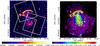 |
Fig. 1 Left: Suzaku observations of CIZA J2242.8+5301 overlaid on a 1.4 GHz radio intensity map in color scale (van Weeren et al. 2010). The Suzaku XIS fields of view are shown as white squares. Right: X-ray image of CIZA J2242.8+5301 in the energy band 0.5−2.0 keV, after subtraction of the NXB with no vignetting correction, after smoothing by a two-dimensional Gaussian with σ = 8 pixel = 8.5′′. The 1.4 GHz radio emission is shown with yellow contours. |
We use H0 = 70 km s-1 Mpc-1, ΩM = 0.27 and ΩΛ = 0.73, which gives a scale of 190 kpc per arcminute at z = 0.192. We employ solar abundances defined by Lodders (2003) and Galactic absorption with NH:total = 46.0 × 1020 cm-2 (Willingale et al. 2013). Unless otherwise stated, the errors correspond to 68% confidence for a single parameter.
2. Suzaku observations and spectrum analysis
Suzaku carried out three observations of CIZA J2242.8+5301 (Fig. 1 left) and one observation of an OFFSET region, during the Suzaku AO-6 (PI: Kawahara) and AO-8 (PI: van Weeren) phase. We refer to these pointings as North, East and South, respectively. They cover the whole cluster beyond the radio relics. The observation log is listed in Table 1. All observations were performed with the normal 5 × 5 and 3 × 3 clocking mode1 (without burst or windows options).
The XIS instrument consists of four CCD chips: one back-illuminated (BI: XIS1) and three front-illuminated (FI: XIS0, XIS2, XIS3) chips (Mitsuda et al. 2007). Because of damage from a meteoroid strike, XIS2 was not operational2. Data reduction was done with HEASOFT version 6.15 and CALDB version 20140203.
The XIS event lists created by the rev 2.5 pipeline processing were filtered using the following additional criteria: a geomagnetic cosmic-ray cut-off rigidity (COR) > 8 GV, and an elevation angle ELV > 12°. We applied additional processing for the XIS1 detector to reduce the non-X-ray background (NXB) level, which increased after the change in the amount of charge injection from 2 keV to 6 keV in June 2011. That operation improved the high-energy response with a negligible loss in low-energy performance3. The detailed processing procedures are the same as those described in XIS analysis topics4. The 5 × 5 and 3 × 3 editing modes data formats were added.
The observed spectrum was assumed to consist of optically-thin thermal plasma emission from the ICM, and emission due to the Galactic foreground, cosmic X-ray background (CXB), and NXB. To investigate the properties of the cluster plasma outside of the radio relics, an accurate estimation of the foreground-background emission is essential. Here we use a Suzaku offset observation, which is located 1 deg east of CIZA J2242.8+5301, to estimate the sky background spectra.
In the fitting procedure for the cluster emission, we combined the spectra from the FI detector (XIS0, 3) and BI and FI spectra were fitted simultaneously. The NXB subtracted spectrum is fitted with a model of the ICM and the sky background components. Details about background estimation and the ICM components across the northern and southern radio relics are described in Sects. 2.1, 2.3 and 2.4.
Suzaku observations log of the CIZA2242.
2.1. Estimation of the background spectra
The sky X-ray background is divided into four components: unabsorbed thermal emission from the local hot bubble (LHB: kT ~ 0.1 keV), absorbed thermal emission form the Milky Way halo (MWH: kT ~ 0.3 keV), the hot foreground (HF: kT ~ 0.6 keV) and the CXB.
To determine the level of the sky X-ray background, we first analyzed a Suzaku offset observation of CIZA J2242.8+5301 (obsID:806002010). We assume that these sky background components are distributed uniformly over the Suzaku FOV. We used uniform ancillary response files (ARF) for the sky background components. The ARF for the sky background was generated using xissimarfgen (Ishisaki et al. 2007), assuming uniform sky emission over a circular region with a radius of 20′. Hereafter, we call this uniform-ARF.
The NXB component was reconstructed from the XIS Night Earth database with xisnxbgen in FTOOLS (Tawa et al. 2008). We accumulated the data for the same detector area and the same distribution of COR2 as the observations. To increase the signal-to-noise ratio, we applied data selection with COR2 > 8 GV (see Fig. 3 in Tawa et al. 2008). To adjust for the long-term variation of the XIS background due to radiation damage, we select the night Earth data within 300 days before and after the period of the observation. Using the wavdetect function in the CIAO package5, we searched for point sources in the Suzaku image. Point sources were detected down to ~1 × 10-13 erg cm-2 s-1 in the 2–10 keV band. We exclude the point sources within a 1−2 arcmin radius to take account for the point spread function (PSF) of the Suzaku XRT (Serlemitsos et al. 2007) into account.
Best-fit background parameters.
For the spectral fits, we used the XSPEC version 12.8.0 package6. The model for the sky-background components is described as ApecLHB + phabs(ApecMWH + ApecHF + powerlawCXB) in XSPEC representation. In this model, Apec and phabs represents thin thermal plasma emission model (Smith et al. 2001) and Galactic absorption toward the target, respectively. We fixed the abundance and the redshift of each thermal component to 1.0 and 0.0, respectively. Further we fixed the temperature of the LHB and photon index of the CXB components to 0.08 keV and Γ = 1.41 (Kushino et al. 2002), respectively. We used the spectra in the 0.5−7 keV range for the BI detectors and 0.8−7 keV for the FI detector. The result is consistent with the CXB intensity with the Kushino et al. (2002) level and the MWH temperature of 0.27 keV is consistent with typical values in other fields (Yoshino et al. 2009). A fit with the HF component fixed to zero (case1) is sightly poorer than a fit with its temperature and nomalization as free parameters (case2). The resulting fit parameters are shown in Table 2. Basically these models reproduce all the features of the observed spectrum well, including CXB intensity, low energy (<1 keV) sky background. We have checked how the HF component improves the fitting with an F-test, and obtained the probability value of the F-test ~0.001. Thus, we employed the parameters of case 2 in Table 2. The best-fit spectrum model (case2) is shown in Fig. 2.
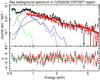 |
Fig. 2 Spectrum of the OFFSET field used for the background estimation, after subtraction of the NXB and the point sources. The XIS BI (Black) and FI (Red) spectra are fitted with CXB + Galactic components (LHB, MWH, and HF) (apec+ phabs(apec+powerlaw+apec)). The CXB spectrum is shown with a black curve, and the LHB, MWH, and HF components are indicated with green, blue and gray curves, respectively. |
2.2. ICM emission along the merging direction
To investigate the cluster temperature distribution in the merging direction (from north to south), we divided the cluster into 11 box regions as shown in Fig. 3. For the ICM emission around the radio relic, we employed an absorbed single temperature thermal plasma model (phabs × apec). In all regions, we fixed the metal abundance and the redshift to 0.3 (Fujita et al. 2008; Werner et al. 2013) and 0.192 (Kocevski et al. 2007), respectively. Because the ICM emission has a different spatial distribution from the sky background, we generated an ARF using the Suzaku XIS image (0.5−8.0 keV band) as the input surface distribution for xissimarfgen. Based on Sect. 2.1, we modeled the sky background emission using the uniform ARF. The XSPEC version 12 enable us to employing multiple ARFs. The normalization of the LHB component, the normalization and temperature of the MWH component, and the normalization of the power-law model for the CXB component were allowed to vary within the range of the errors in the background estimation (Table 2). We separately carried out spectral fits to the pulse-height spectra in each annular region. We only allowed the normalizations to differ in the simultaneous fit of the BI and FI data, although we found that the derived normalizations were consistent within 15%. The resulting temperature profile is shown in Fig. 3. The temperature profile shows a significant drop at r = −6 and 6 arcmin, respectively. The temperature drop strongly indicates the presence of shock fronts at those locations. Here we note that the temperature profile was smeared by the point spread function of the Suzaku XRT (half power diameter ~2 arcmin: Serlemitsos et al. 2007). Therefore, we can not resolve structures of scales less than an arcmin. In the next section, we investigate in detail the properties around the radio relics.
2.3. ICM emission across the northern radio relic
To investigate the detailed ICM properties associated with the radio relics, we extracted pulse-height spectra in two annular regions whose boundary radii were 4.0′−7.0′ and 7.5′−11.5′ for the region inside and outside the radio relic with the center at (22:42:41.9, 53:03:00.0); this is shown in Fig. 5. To reduce contamination from the brighter region, we take the region outside the radio relic 0.5′ away from the outer edge of the inner region. To maximize the signal-to-noise ratio outside the northern relic region, we used the spectra in the 0.5–4 keV range for the BI detector and 0.8–4 keV for the FI detectors.
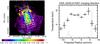 |
Fig. 3 Left: X-ray image of the CIZA J2242.8+5301 in the energy band 0.5−5.0 keV, after subtraction of the NXB with no vignetting correction and after smoothing by a two dimensional Gaussian with σ = 8 pixel = 8.5′′. The identified point sources by XMM-Newton are highlighted with the green circles (see text). The 1.4 GHz radio emission is shown with yellow contours. The dashed cyan circle indicate the center which, was determined by visually fitting a circle to the radio relics. Right: temperature profile of CIZA J2242.8+5301 from the south to north direction. The dotted gray lines show WSRT 1.4 GHz radio emission. |
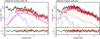 |
Fig. 4 NXB subtracted spectra in each annular region. The XIS BI (Black) and FI (Red) spectra are fitted with the ICM model (phabs × apec), along with the sum of the CXB and the Galactic emission of Case 2 (apec + phabs(apec + apec + powerlaw)). The ICM component is shown with a magenta line. The CXB component is shown with a black curve, and the LHB, MWH, and HF emissions are indicated with green, blue and gray curves, respectively. The sum of all sky background components is shown with the orange curve. The left panel shows the spectrum of the outside region. The right panel shows the inside region. |
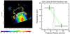 |
Fig. 5 Left: Suzaku XIS image for the northern part of CIZA J2242.8+5301. Right: radial profile of the ICM temperature for the north direction. The present best-fit values with statistical errors are shown with black crosses. Gray dotted crosses indicate previous Suzaku results, which do not include HF component (Akamatsu & Kawahara 2013). The range of uncertainties due to the combined 3% variation of the NXB level and the maximum/minimum fluctuation in the CXB is shown with two green dashed lines. The black dotted lines show the WSRT 1.4 GHz radio intensity scaled arbitrary in flux. The higher peak corresponds the northern radio relic and the second peak is a point source just behind the radio relic. |
To investigate a possible systematic error in the temperature estimation, we consider a 3% fluctuation of the NXB level and fluctuations of the CXB intensity as shown below. It is important to exclude the contribution of point sources in the region of interest, and to reduce the systematic error of the CXB caused by fluctuations of unresolved sources. For the elimination of the point sources, we used the archival data of XMM-Newton (OBSID=0654030101). As shown with small (green) circles in Fig. 3, we detected several point sources and subtracted 10 point sources with 2.0−10.0 keV fluxes higher than Sc = 1 × 10-14 erg cm-1 s-1. According to previous studies of the CXB with the ASCA satellite (Kushino et al. 2002), the CXB flux fluctuation in the field of view of the ASCA GIS (0.5 deg2) is 6.5% in the 2−10 keV band. We scaled the measured fluctuations from our flux limit and the observed area following Hoshino et al. (2010). The estimated fluctuations are 32% and 18% for inside and outside of the radio relic regions, respectively. We repeated all the spectral fits by fixing the CXB intensity at the upper and lower boundary values.
The pulse-height spectra and the best-fit models for both annular regions are shown in Fig. 4. We obtained fairly good fits for all the regions with reduced χ2 values less than 1.2. The resultant ICM temperature with different background models are listed in Table 5. The temperature changes significantly from  keV to
  keV. Even though we use different sky background models, these results are consistent with previous Suzaku results (kTinside = 8.3 ± 0.8 keV and kToutside = 2.1 ± 0.4 keV: Akamatsu & Kawahara 2013). These ICM temperatures are consistent with these estimated from the box regions shown in Fig. 3.
For the inside and outside the northern relic, the box region shows kTinside = 9.7 ± 1.3 keV and kToutside = 3.4 ± 1.1 keV, respectively. The ICM temperature of the post-shock region also agrees with a previous XMM-Newton observation (kTinside ~ 8−11 keV: Ogrean et al. 2013). Figure 5 shows the radial profile of the ICM temperature across the northern radio relic. Black crosses show the best-fit ICM temperature of each annular region. Gray dotted crosses represent previous results (Akamatsu & Kawahara 2013), which do not include the HF component.
One can also estimate the shock compression from the jump in the X-ray surface brightness across the relic. The surface brightness was derived from the observed spectra. We checked the surface brightness across the well-defined northern radio relic. The resulting unabsorbed X-ray surface brightness (0.5−2.0 keV) shows a factor 8 difference across the relic, which corresponds to a shock compression of  , including the difference in emissivity for the two regions. This value matches the compression parameter (
 ) derived across the rectangular sector, which is shown Fig. 3. These surface brightness jumps are consistent with the shock compression predicted based on the temperature jump (Table 5:
  ). This agrees with the results for shocks found on other clusters (for instance, Bullet: Markevitch et al. 2002 Shimwell et al. 2015; A520: Markevitch et al. 2005; A754: Macario et al. 2011; RXJ 1314.4-2515 Mazzotta et al. 2011). However, we note that our estimation based on our X-ray spectroscopic analysis represent the upper limit to the density jumps because the surface brightness profiles of clusters of galaxies typically have steep power-law profiles. It is difficult to make concrete statements on this issue because of the limited spatial resolution of the Suzaku XRT.
Best-fit ICM temperature across the northern radio relic with different background models (unit of keV).
2.4. ICM emission around the southern radio relic
Next we investigate the ICM properties around the southern radio relic with our new Suzaku observations. To increase the signal with our limited observation time, the west and east observations overlap at the southern radio relic. We analyzed these data in the same way as the northern one. Similar to the northern relic, we take a one arcmin gap to avoid contamination from the brighter part of the cluster due to the PSF of the Suzaku XRT. To investigate possible structures in the W and E directions, we also evaluate the ICM temperatures by shifting the annuli by 0.5′. The resulting ICM temperatures are shown with the gray crosses in the Fig. 7.
We used the spectra in the 0.5–7 keV range for the BI detectors and 0.8–7 keV for the FI detector. For point source exclusion, we only used Suzaku data because XMM-Newton/Chandra observations did not completely cover the full Suzaku FOV. We excluded point sources using CIAO to a flux detection limit of Sc = 1 × 10-13 erg cm-2 s-1. Based on the flux detection limit, we estimate the possible fluctuation of the CXB intensity in each region. The estimated fluctuations span 35−60%.
Best-fit ICM temperature across the southern radio relic with different background models (unit of keV).
We successfully obtained the ICM temperature across and beyond the south relic for the first time. The resulting ICM temperature across the radio relic region is shown in Table 4. The best-fit temperature profiles are shown in Fig. 7. Toward the southern radio relic, the ICM temperature shows slightly increasing profile from 8.0 ± 0.3 keV to 9.0 ± 0.5 keV and shows a significant drop to 5.0 keV. Similar to the results for the northern shock/relic, these temperatures are consistent with those derived for in the rectangular sector (Fig. 3), although the statistical errors are large. This might be because this region is located too far from the radio relic, and the bin is placed at about 760 kpc from the peak of radio emission. Given the expected decrease in temperature with radius this would explain the lower temperature measured there. Combined with the fluctuation of the NXB level (3%: Tawa et al. 2008), we investigated the systematic error. The results are shown with green dotted lines in Fig. 7. Because of the high point source flux detection limit, the fluctuations of the CXB intensity are large. The emission intensity outside of the southern radio relic is almost comparable to the sky background (Fig. 6). Therefore, the systematic errors outside of the southern radio relic are larger than the statistical error.
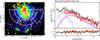 |
Fig. 6 Radial profile of the ICM temperature for the southern direction. Colors are the same as in Fig. 5. |
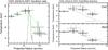 |
Fig. 7 Radial profile of the ICM temperature for the south (left), east and west direction. The black crosses show the best-fitted values and the gray crosses show the results of slightly offset regions. The gray dotted curves in the right panels show the temperature profile Burns et al. (2010; see text). In the left panel, we removed the radio point sousrce located just behind the relic. |
3. Discussion
We performed deep Suzaku observations of the double radio relic cluster CIZA J2242.8+5301. The ICM temperature profiles beyond the relics were measured. The profiles show a significant drop across the radio relics, which implies the presence of shock fronts. We discuss the full cluster temperature structure by comparing to other clusters. We evaluate the shock properties (Mach number, compression factor and propagation speed), the possibility of nonequilibrium effects due to shock heating and we compare these results with the radio observations.
Shock properties at the northern and southern radio relic.
3.1. Large-scale ICM temperature structure
As suggested by numerical simulations, clusters grow via merging with subclusters. These merging activities have a huge impact on the temperature structure (see for a review Markevitch & Vikhlinin 2007). Recent Suzaku observations reveal the ICM temperature profiles up to the virial radius (see for a review Reiprich et al. 2013). However, these studies mainly focus on relaxed clusters, and studies of merging cluster outskirts are still limited except for a few examples (e.g., Ibaraki et al. 2014). Therefore, the impact of merging activity on the cluster structure remains poorly known.
The new Suzaku observations of CIZA J2242.8+5301, in combination with Suzaku observations taken in 2011 (Akamatsu & Kawahara 2013), cover the full cluster region. As shown in Fig. 3, CIZA J2242.8+5301 has a peculiar temperature profile along the merging axis (from north to south). Contrary to relaxed clusters (Reiprich et al. 2013), CIZA J2242.8+5301 has an almost flat radial profile with kT ~ 8 keV (Ogrean et al. 2013, and this work). In addition, across the radio relics, the temperature profile also shows a significant drop. These observed temperature profiles strongly indicate the presence of a shock front and shock heating on the ICM. We discuss the properties of the shock fronts in the next subsection.
We plotted a model temperature profile proposed by Burns et al. (2010) as gray dotted curves in the right panel of Fig. 7. Their model profile reproduces well the measured ICM temperature structure of relaxed clusters of galaxies by the Suzaku satellite (Reiprich et al. 2013). For the calculation of the model profile, we adopt Tavg = 8.0 keV and r200 = 12 arcmin, respectively. Here, r2007 is estimated from Henry et al. (2009). We also compare the measured temperature profiles with previously measured clusters (Fig. 8). The temperature profile in the W direction agrees with the model profile. On the other hand, the profile in the E direction shows an excess. The temperature excess in the E direction is consistent with the previous XMM-Newton results (Ogrean et al. 2013). They report the presence of a high temperature (kT ~ 13 keV) region at the eastern part of the cluster. In our temperature profile, we do not find a temperature region this high. However, because of the limited PSF of the Suzaku XRT, we may miss this component. In addition, a high temperature (kT> 10 keV) like this is beyond the effective energy band of XIS and of XMM-Newton. Therefore tight constraints on high temperature components are difficult to obtain for current X-ray CCD detectors. NuSTAR8 (Harrison et al. 2010) and the upcoming ASTRO-H9 (Takahashi et al. 2012) satellite will help to detect such high temperature components with their hard X-ray imaging and spectral capabilities.
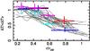 |
Fig. 8 Scaled projected temperature profiles compared with relaxed clusters (gray: see Fig. 8 in Reiprich et al. 2013). The profiles were normalized to the average temperature. The r200 value was derived from Henry et al. (2009). Blue, red, yellow and magenta crosses show the temperature profile of the North, South, East and West direction, respectively. |
3.2. Shock properties
The Suzaku temperature profiles of CIZA J2242.8+5301 show clear drops across the relics, indicating the presence of shock fronts. We evaluate the shock properties at both radio relics based on the Suzaku results. Hereafter we used the error including systematic errors due to the variation of the NXB level and the maximum/minimum fluctuation in the CXB defined as  We cannot determine a one-to-one relationship between the edge of the radio relics and the shock fronts because of the limited PSF of the Suzaku XRT.
The Mach number can be obtained by applying the Rankine-Hugoniot jump condition (Landau & Lifshit’s 1959)  (1)assuming the ratio of specific heats as γ = 5/3. Here, 1,2 indicate pre-shock and post-shock, respectively. Table 5 shows the resultant Mach numbers based on the temperature jump, whose values are
  ,
,  , respectively (Table 5).
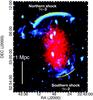 |
Fig. 9 Smoothed 0.5−2.0 keV band X-ray image (red) and WSRT 1.4 GHz image of CIZA J2242.8+5301 (cyan). The thin yellow lines depict the approximate locations of the shock fronts confirmed by Suzaku. |
Using the measured temperature in the pre-shock region (kTpre:n ~ 2.7 keV, kTpre:s ~ 5.1 keV), the sound speed is cs:n ~ 850 km s-1, cs:s ~ 1170 km s-1. With these Mach numbers, the expected shock compression C and the shock propagation speed (vshock = ℳ·cs) are estimated as  ,
,  and
and  ,
,  , respectively. For the northern radio relic, the estimated shock speed is in agreement with the radio observations (vshock:n ~ 2500 km s-1: Stroe et al. 2014a). Here we estimate the shock compression C from the Mach numbers derived from the temperature drops. Although the Mach number is comparable to that of the Bullet cluster (ℳ ~ 3.0), the shock velocity in CIZA J2242.8+5301 is much smaller than for the Bullet cluster (4500 km s-1) and is comparable to A520 (2300 km s-1) and other systems (e.g. A2034: 2057 km s-1). The relative gas flow speed to the shock front is vgas:n = vshock/C ~ 810 km s-1 and vgas:s ~ 1000 km s-1. The estimated downstream velocity for the northern shock is in agreement with that used for estimating the magnetic field (vgas = 1000 km s-1,
  : van Weeren et al. 2010; Stroe et al. 2014a).
Here we discuss possible systematics on our estimate of pre-shock temperature. The Mach number we determined is in principle also affected by any temperature gradient that was present before the shock passage. Any shock heating appears as an excess above the temperature gradient that was already present. We can provide an approximate estimate of this effect assuming the gradient before shock passage followed the profile from Burns et al. (2010). Substituting an average temperature of ⟨ kT ⟩ = 8 keV into Eq. (8) of Burns et al. (2010), the expected temperature gradient between the center of pre- and post-shock is 2.0 keV. So the temperature at the current post-shock location, but before shock passage, was about 2.7 + 2.0 = 4.7 keV. After passage of the shock this increased to the currently measured post-shock value of 8.5 keV. With a value of T1 = 4.7 keV and T2 = 8.5 keV this corresponds to a Mach number of 1.8.
Additional uncertainties arise from the fact that we assumed the temperature measurements are valid for the center of the bins in the above calculation. Our actual temperature estimate is emission weighted, resulting in a temperature bias in the high-density region. Therefore, the position of the weighted temperature of the pre-shock bin could actually be located closer to the relic position (see Fig. 6 in Hoshino et al. 2010) and the shock heating is expected to be located at the edge of the relic. Due to this fact, the correction for the pre-shock temperature is likely somewhat smaller than what we assumed above. As an example, the expected temperature gradient between the edge of the relic and the center of the pre-shock region is ~0.8 keV, assuming the same Burns et al. (2010) profile. The expected pre-shock temperature precisely at the edge of the shock would then be 2.7 + 0.8 = 3.5 keV. With our measured post-shock temperature, this would then correspond to a Mach number of 2.3. We stress that the above calculations are just estimates as we lack information on the original temperature profile before the merger. The discussion in the following sections and conclusions are not affected by this systematics.
3.3. Merger scenario of CIZA J2242.8+5301
The temperature distribution of the ICM shown in Figs. 3, 5, 7 and the presence of the shock fronts suggest that a subcluster is colliding into the main body from the north-south direction. The peak of X-ray emission is close to the southern part of the cluster (Ogrean et al. 2013, 2014), which might be infalling from the north direction. In this point of view, the northern shock corresponds to the backward shock induced by the merging activity. We do not see a significant excess in the temperature profile in the perpendicular direction to the merger axis, which is predicted by several simulations (Akahori & Yoshikawa 2010; Molnar et al. 2013). Overall, our observations indicate that CIZA J2242.8+5301 is experiencing an almost head-on merger with near unity mass ratio and small impact parameter.
Here we estimate the dynamical timescale of CIZA J2242.8+5301, using its shock properties and radio information. Assuming that the shock propagation speed does not change from vshock ~ 2000 km s-1 and that the distance from the north to the south relic is 2.5 Mpc, we estimate that CIZA J2242.8+5301 is observed approximately 2.5 Mpc/(2 × vshock) ~ 0.6 Gyr after core passage. Note that the actual timescale is expected to be longer as the shock speed just after core passage is lower. Therefore, the total travel time would be longer than 0.6 Gyr. Our results support previous estimates based on hydrodynamical simulation and radio observations (van Weeren et al. 2011; Stroe et al. 2014a). They suggested that CIZA J2242.8+5301 is a binary cluster merger with a mass ratio of 1:2, less than 10 degrees from the plane of the sky and impact parameter b< 400 kpc. The combination of radio and X-ray observations is powerful to constrain cluster merger events. For a more detailed understanding of the dynamical evolution of the merger, the mass distribution from a weak lensing observation and hydrodynamical simulations are useful (e.g., Dawson 2013).
3.4. Mach number from X-ray and radio observations
Recent X-ray follow-up observations of the radio relics reveal a relation between the shock front and radio emission (Finoguenov et al. 2010; Macario et al. 2011; Mazzotta et al. 2011; Ogrean et al. 2013; Ogrean & Brüggen 2013; Akamatsu & Kawahara 2013). These results are consistent with the hydrodynamical simulations of merging clusters, which predict that merging events generate shock waves toward outskirts (Takizawa & Mineshige 1998; Ricker & Sarazin 2001; Kang et al. 2005). These shocks accelerate electrons up to relativistic energies via diffusive shock acceleration (DSA) mechanism, which generates radio emission via synchrotron radiation. However, as mentioned in the introduction, the acceleration efficiency of DSA with low-ℳ (<10) shocks is known to be too low to account for the radio flux. Therefore the main acceleration mechanism at cluster merger shocks is still unclear and until now the subject of discussion. To understand shock acceleration, it is crucial to know the particle acceleration efficiency and injection rate.
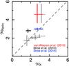 |
Fig. 10 Mach number derived from radio (Mradio) plotted against that from the ICM temperature. The error bars are only statistical and at the one sigma level. Red and blue crosses are this work, but with previous and new radio result (van Weeren et al. 2010; Stroe et al. 2014b). Grsy crosses show the previous our results (Akamatsu & Kawahara 2013). Note: Stroe et al. (2014a) does not give information about the southern relic because the low flux. Therefore the result of the new radio analysis is only available for the northern relic. However, similar to the northern relic case, the Mach number of the southern radio relic is expected to drop. |
Because of the presence of the two clear and giant radio relics, CIZA J2242.8+5301 is one of the best targets to study shock acceleration in clusters. Especially, the northern relic shows an extremely narrow shape, whose width is only 50 kpc (Fig. 1). van Weeren et al. (2010), Stroe et al. (2013) reported the spectral index map of the radio relics in CIZA J2242.8+5301. At the edge of the northern radio relic, the spectral index is estimated from the spectral index map and color–color diagram as αn = −0.6 ± 0.05, which correspond to the Mach number of  . They also confirm the presence of a spectral index gradient across the relic, which is consistent with the DSA theory combined with Synchrotron aging. On the other hand, for the southern radio relic, it was not possible to estimate the injection spectral index directly from spectral index maps due to poor signal to noise. Therefore, the estimated injection spectral index from the measured integrated spectral index αint = −1.29 ± 0.05 as αinj = −0.79 ± 0.05, which corresponds to a Mach number of ℳ = 2.8 ± 0.2 (Stroe et al. 2013). We note that the estimated injection spectral index remains uncertain because of the assumptions that have to be made if it is derived from the integrated spectrum (Kang 2015a,b). The new results of the radio analysis (Stroe et al. 2014a) is slightly different from the previous result (αn ~ −0.6: van Weeren et al. 2010; Stroe et al. 2013). The main difference is that Stroe et al. (2014a) used a largest radio data set and took spatial convolution effects into account. Because of the low flux of the southern radio relic, Stroe et al. (2014a) could not estimate the spectral index. Therefore the result from the new radio analysis is only available for the northern relic.
First order Fermi acceleration (under the assumptions of stationary and continuous injection) yields relativistic electrons with a power-law spectrum n(E)dE ~ E− pdE, where the power-law index is p = (C + 2)/(C − 1). The radio spectral slope just after the shock acceleration is α = −(p−1)/2. Using the measured shock compression, this relation implies pn = 2.64 ± 0.30,  and αn = −0.81 ± 0.15,
  , respectively. For the northern radio relic, the above value is consistent with the spectral index from the radio investigation (van Weeren et al. 2010; Stroe et al. 2014a, α ~ −0.6 ± 0.05, α ~ −0.77). For the DSA theory, the measured injection index would require a shock compression of Cn ~ 2.84, that again consistent with what is suggested by the temperature drop across the radio relic (Table 5: Cn ~ 2.8).
Although it is likely to change similar to the northern radio relic case, there is a difference between the X-ray and radio measurement of the southern radio relic. Using the measured integrated spectral index and an assumption for the cooling effect, a similar trend has been seen in several radio relics and edges of the halo (Markevitch et al. 2005; Ogrean & Brüggen 2013; Ogrean et al. 2013; Akamatsu et al. 2013). There are several mechanism proposed to explain the particle acceleration in clusters (Markevitch et al. 2005; Kang et al. 2012; Pinzke et al. 2013; Skillman et al. 2013). A plausible possibility is re-acceleration of pre-existing nonthermal (low-energy cosmic-ray) particles in the ICM. In this case, the pre-shock ICM already contains several type of nonthermal particles, which are generated by several mechanisms such as large-scale accretion shock (Ryu et al. 2003), turbulence acceleration (Brunetti 2011) and past activity of radio or starburst galaxies (see Brüggen et al. 2012, for a review). These low-energy cosmic-ray particles have a long lifetime comparable to the ages of clusters or longer (Sarazin 1999; Pinzke et al. 2013). Recently, Kang et al. (2012) performed time-dependent simulations for diffusive shock acceleration for the case of the northern radio relic in CIZA J2242.8+5301. Compared with the observed synchrotron flux and spectral distributions, they concluded that if a pre-existing population of low-energy cosmic-ray electrons exists, the radio relics can be explain by weak shocks with a Mach number ℳ ~ 2−3. A similar conclusion is also reported by Pinzke et al. (2013). They found that contributions of fossil electrons cannot be ignored for low Mach number shocks and their self-similar analytic model described the observed radio properties well. Another possibility is that of a varying Mach number along the shock. The ICM in the cluster outskirts is thought to be clumpy (Nagai & Lau 2011; Simionescu et al. 2011), the inhomogeneities in the ICM thus results in small Mach number variations which could lead to a discrepancy between the radio and X-ray derived Mach numbers as the shock acceleration efficiency (and radio relic brightness) scales nonlinearly with Mach number (Hoeft & Brüggen 2007).
For CIZA J2242.8+5301, we measured the ICM temperature jump across the northern relic, which corresponds to a Mach number of ℳ ~ 3. Indeed, the latest radio investigations by Stroe et al. (2014a) suggest that the previous radio spectral index might be biased and that the estimated spectral index is α ~ −0.77, which corresponds to a Mach number ℳ ~ 3.0. The new Mach number from radio observation agrees well with X-ray observations. In addition, the measured Mach number matches the prediction of the simulation by Kang et al. (2012). This supports the scenario of re-acceleration of the pre-existing nonthermal particles in the ICM. Upcoming LOFAR low-frequency radio observations will shed new light on this problem. This kind of high-quality radio spectrum allows us to observe the injection spectral index directly.
3.5. Magnetic field pressure at the northern radio relic
As suggested by previous radio observations (van Weeren et al. 2010), the northern relic has a relatively high magnetic field (B ~ 5 μG). Similar results are also reported for other radio relics (Nakazawa et al. 2009). This kind of magnetic field strength is comparable to the expected value at the cluster central region from simulations of the Faraday rotation measure in the Coma cluster (Bonafede et al. 2010).
The thermal pressure of the ICM and the magnetic pressure of relativistic electrons is calculated as Pth = kT·ne and Pmagnetic = B2/ (8π), respectively. Assuming the ICM temperature and electron density kT ~ 8.0 keV and ne ~ 5 × 10⁻⁴ cm-3, we estimate the thermal pressure at the northern radio relic Pth ~ 6.7 eV/cm3, assuming that the mean molecular weight is 0.6. Here we assume that all X-ray emission comes from the thermal component. With a magnetic field strength of B ~ 5 μG, the energy density is estimated as Pmagnetic ~ 0.62 eV/cm3. Comparing both pressures, we find that the magnetic pressure reaches ~9% of the thermal pressure. In the above estimate, we did not include the contribution of the energy density of the nonthermal electrons and turbulence. Therefore, PB/Pth ~ 0.09 is a robust lower limit of the nonthermal pressure.
3.6. Possibility of nonequilibrium effects
Finally we discuss the possibility of nonequilibrium effects. Similar to supernova remnants, cluster merger shocks are expected to be collisionless. In the shock in young supernova remnants, there is a well-known relation between the ratio of the ion and electron temperature Te/Ti and shock velocity as  (van Adelsberg et al. 2008). In the cluster case, nonequilibrium effects such as non-Maxwellian electron distributions (Kaastra et al. 2009), nonequipartition of electrons and ions temperature (Takizawa 2005; Rudd & Nagai 2009; Akahori & Yoshikawa 2010), and nonequilibrium ionization are also expected.
Because of the different mass between the ions and the electrons, in general, shock heating is more effective for the ions. The electrons set the same temperature via Coulomb collisions. After that, electrons stabilize down to a Maxwellian distribution. Finally, via ion-to-ion collisions, the ionization balance in the ICM reaches equilibrium. The collisional timescale is given by netie = 3 × 1011 cm-3 s. Here, netie is the ionization parameter, which is an indicator of the ionization degree (Masai 1984). The region just behind the shock may have a higher ion temperature Ti than the electron one Te because it has not had enough time to reach equilibrium. We also tried to evaluate the ionization parameter net at the post-shock region using the NIE model in Xspec. Unfortunately Suzaku can not constraint well the net parameter because of the low abundance and low statistics of Fe–K lines. Further studies should be possible by high-resolution spectroscopy of the ICM with the Japanese ASTRO-H (Takahashi et al. 2012) and the European ATHENA10 (Nandra et al. 2013) satellites.
4. Summary
CIZA J2242.8+5301 (z = 0.192) hosts two well-defined giant radio relics. We find that the temperature profiles show a remarkable drop across both relics. Below is a summary of our main results:
The ICM temperature of the merging direction shows a flat profile with kT ~ 8 keV and shows a clear drops to 3−5 keV across the radio relics. The ICM temperature of the perpendicular direction to the merging axis shows different profiles. The temperature profile in the western direction agrees with the simulated temperature profile of Burns et al. (2010). The significant drop in the ICM temperature indicates the presence of shock fronts. Based on the temperature drop, the estimated Mach number of the shocks are  , and
, and  , respectively. The shock velocities are also estimated as vshock:n ~ 2300 km s-1 and vshock:s ~ 2000 km s-1, respectively. This suggests that the merger happened ~0.6 Gyr ago, in agreement with estimates based on hydrodynamical simulation and dynamical analysis (van Weeren et al. 2011; Stroe et al. 2014a; Dawson et al., in prep.). The observed radio spectral index of the northern relic (Stroe et al. 2014a) is consistent with what would be expected from diffusive shock acceleration in a shock with the observed Mach number and compression. By combining our X-ray data with radio results, we estimated the fraction of the magnetic pressure to the thermal pressure at the northern radio relic to be about ~0.62 eV/cm3, which corresponds to 9% of the thermal pressure.
r200 is the radius where the mean total density of the cluster is 200 times the mass density of the Universe with critical density.
Acknowledgments
The authors wish to thank the referee for constructive comments that significantly improved the manuscript. The authors thank the Suzaku team members for their support of the Suzaku project and T. H. Reiprich for the data to reproduce temperature profiles obtained with Suzaku. We would also like to thank A. Simionescu and K. Sato for useful discussions. H.A. is supported by a Grant-in-Aid for Japan Society for the Promotion of Science (JSPS) Fellows (26-606). R.J.W. is supported by NASA through the Einstein Postdoctoral grant number PF2-130104 awarded by the Chandra X-ray Center, which is operated by the Smithsonian Astrophysical Observatory for NASA under contract NAS8-03060. H.K. is supported by the Astrobiology Project of the CNSI, NINS (AB261006) and by Grant-in-Aid for Scientific research from JSPS and from the MEXT (No. 25800106). A.S. acknowledges financial support from NWO. D.S. acknowledges financial support from the Netherlands Organisation for Scientific research (NWO) through a Veni fellowship, from FCT through a FCT Investigator Starting Grant and Start-up Grant (IF/01154/2012/CP0189/CT0010) and from FCT grant PEst-OE/FIS/UI2751/2014. M.H. acknowledges financial support by the DFG, in the framework of the DFG Forschergruppe 1254 “Magnetisation of Interstellar and Intergalactic Media: The Prospects of Low-Frequency Radio Observations”. G.A.O. acknowledges support by NASA though a Hubble Fellowship grant HST-HF2-51345.001-A awarded by the Space Telescope Science Institute, which is operated by the Association of Universities for Research in Astronomy, Inc., under NASA contract NAS5-26555. SRON is supported financially by NWO, the Netherlands Organization for Scientific Research.
References
- Akahori, T., & Yoshikawa, K. 2010, PASJ, 62, 335 [NASA ADS] [Google Scholar]
- Akamatsu, H., & Kawahara, H. 2013, PASJ, 65, 16 [NASA ADS] [CrossRef] [Google Scholar]
- Akamatsu, H., de Plaa, J., Kaastra, J., et al. 2012a, PASJ, 64, 49 [NASA ADS] [Google Scholar]
- Akamatsu, H., Takizawa, M., Nakazawa, K., et al. 2012b, PASJ, 64, 67 [NASA ADS] [Google Scholar]
- Akamatsu, H., Inoue, S., Sato, T., et al. 2013, PASJ, 65, 89 [NASA ADS] [Google Scholar]
- Blandford, R., & Eichler, D. 1987, Phys. Rep., 154, 1 [Google Scholar]
- Bonafede, A., Feretti, L., Murgia, M., et al. 2010, A&A, 513, A30 [NASA ADS] [CrossRef] [EDP Sciences] [Google Scholar]
- Bourdin, H., Mazzotta, P., Markevitch, M., Giacintucci, S., & Brunetti, G. 2013, ApJ, 764, 82 [NASA ADS] [CrossRef] [Google Scholar]
- Brüggen, M., Bykov, A., Ryu, D., & Röttgering, H. 2012, Space Sci. Rev., 166, 187 [Google Scholar]
- Brunetti, G. 2011, Mem. Soc. Astron. It., 82, 515 [NASA ADS] [Google Scholar]
- Brunetti, G., & Jones, T. W. 2014, Int. J. Mod. Phys. D, 23, 30007 [Google Scholar]
- Burns, J. O., Skillman, S. W., & O’Shea, B. W. 2010, ApJ, 721, 1105 [Google Scholar]
- Dawson, W. A. 2013, ApJ, 772, 131 [NASA ADS] [CrossRef] [Google Scholar]
- Ensslin, T. A., Biermann, P. L., Klein, U., & Kohle, S. 1998, A&A, 332, 395 [NASA ADS] [Google Scholar]
- Feretti, L., Giovannini, G., Govoni, F., & Murgia, M. 2012, A&ARv, 20, 54 [Google Scholar]
- Finoguenov, A., Sarazin, C. L., Nakazawa, K., Wik, D. R., & Clarke, T. E. 2010, ApJ, 715, 1143 [NASA ADS] [CrossRef] [Google Scholar]
- Fujita, Y., Tawa, N., Hayashida, K., et al. 2008, PASJ, 60, 343 [Google Scholar]
- Guo, X., Sironi, L., & Narayan, R. 2014a, ApJ, 794, 153 [NASA ADS] [CrossRef] [Google Scholar]
- Guo, X., Sironi, L., & Narayan, R. 2014b, ApJ, 797, 47 [NASA ADS] [CrossRef] [Google Scholar]
- Harrison, F. A., Boggs, S., Christensen, F., et al. 2010, in SPIE Conf. Ser., 7732 [Google Scholar]
- Henry, J. P., Evrard, A. E., Hoekstra, H., Babul, A., & Mahdavi, A. 2009, ApJ, 691, 1307 [NASA ADS] [CrossRef] [Google Scholar]
- Hindson, L., Johnston-Hollitt, M., Hurley-Walker, N., et al. 2014, MNRAS, 445, 330 [NASA ADS] [CrossRef] [Google Scholar]
- Hoeft, M., & Brüggen, M. 2007, MNRAS, 375, 77 [NASA ADS] [CrossRef] [Google Scholar]
- Hoshino, A., Henry, J. P., Sato, K., et al. 2010, PASJ, 62, 371 [NASA ADS] [CrossRef] [Google Scholar]
- Ibaraki, Y., Ota, N., Akamatsu, H., Zhang, Y.-Y., & Finoguenov, A. 2014, A&A, 562, A11 [NASA ADS] [CrossRef] [EDP Sciences] [Google Scholar]
- Ishisaki, Y., Maeda, Y., Fujimoto, R., et al. 2007, PASJ, 59, 113 [NASA ADS] [Google Scholar]
- Itahana, M., Takizawa, M., Akamatsu, H., et al. 2015, PASJ, submitted [arXiv:1508.05845] [Google Scholar]
- Kaastra, J. S., Bykov, A. M., & Werner, N. 2009, A&A, 503, 373 [NASA ADS] [CrossRef] [EDP Sciences] [Google Scholar]
- Kang, H. 2015a, J. Korean Astron. Soc., 48, 9 [NASA ADS] [CrossRef] [Google Scholar]
- Kang, H. 2015b, J. Korean Astron. Soc., 48, 155 [NASA ADS] [CrossRef] [Google Scholar]
- Kang, H., Ryu, D., Cen, R., & Song, D. 2005, ApJ, 620, 21 [NASA ADS] [CrossRef] [Google Scholar]
- Kang, H., Ryu, D., & Jones, T. W. 2012, ApJ, 756, 97 [Google Scholar]
- Kocevski, D. D., Ebeling, H., Mullis, C. R., & Tully, R. B. 2007, ApJ, 662, 224 [NASA ADS] [CrossRef] [Google Scholar]
- Koyama, K., Petre, R., Gotthelf, E. V., et al. 1995, Nature, 378, 255 [NASA ADS] [CrossRef] [Google Scholar]
- Kravtsov, A. V., & Borgani, S. 2012, ARA&A, 50, 353 [NASA ADS] [CrossRef] [Google Scholar]
- Kushino, A., Ishisaki, Y., Morita, U., et al. 2002, PASJ, 54, 327 [NASA ADS] [CrossRef] [Google Scholar]
- Landau, L. D., & Lifshit’s, E. M. 1959, Theory of elasticity (London: Pergamon Press) [Google Scholar]
- Lodders, K. 2003, ApJ, 591, 1220 [NASA ADS] [CrossRef] [Google Scholar]
- Macario, G., Markevitch, M., Giacintucci, S., et al. 2011, ApJ, 728, 82 [NASA ADS] [CrossRef] [Google Scholar]
- Markevitch, M. 2010, Review talk at 12th Marcel Grossman Meeting, Paris, July 2009, ArXiv e-prints [arXiv:1010.3660] [Google Scholar]
- Markevitch, M., & Vikhlinin, A. 2007, Phys. Rep., 443, 1 [NASA ADS] [CrossRef] [EDP Sciences] [Google Scholar]
- Markevitch, M., Gonzalez, A. H., David, L., et al. 2002, ApJ, 567, L27 [NASA ADS] [CrossRef] [Google Scholar]
- Markevitch, M., Govoni, F., Brunetti, G., & Jerius, D. 2005, ApJ, 627, 733 [NASA ADS] [CrossRef] [Google Scholar]
- Masai, K. 1984, Ap&SS, 98, 367 [NASA ADS] [CrossRef] [Google Scholar]
- Mazzotta, P., Bourdin, H., Giacintucci, S., Markevitch, M., & Venturi, T. 2011, Mem. Soc. Astron. It., 82, 495 [NASA ADS] [Google Scholar]
- Miniati, F., Ryu, D., Kang, H., et al. 2000, ApJ, 542, 608 [NASA ADS] [CrossRef] [Google Scholar]
- Mitsuda, K., Bautz, M., Inoue, H., et al. 2007, PASJ, 59, 1 [Google Scholar]
- Molnar, S. M., Chiu, I.-N. T., Broadhurst, T., & Stadel, J. G. 2013, ApJ, 779, 63 [NASA ADS] [CrossRef] [Google Scholar]
- Nagai, D., & Lau, E. T. 2011, ApJ, 731, L10 [NASA ADS] [CrossRef] [Google Scholar]
- Nakazawa, K., Sarazin, C. L., Kawaharada, M., et al. 2009, PASJ, 61, 339 [NASA ADS] [Google Scholar]
- Nandra, K., Barret, D., Barcons, X., et al. 2013, ArXiv e-prints [arXiv:1306.2307] [Google Scholar]
- Ogrean, G. A., & Brüggen, M. 2013, MNRAS, 433, 1701 [NASA ADS] [CrossRef] [Google Scholar]
- Ogrean, G. A., Brüggen, M., Röttgering, H., et al. 2013, MNRAS, 429, 2617 [NASA ADS] [CrossRef] [Google Scholar]
- Ogrean, G. A., Brüggen, M., van Weeren, R., et al. 2014, MNRAS, 440, 3416 [NASA ADS] [CrossRef] [Google Scholar]
- Owers, M. S., Nulsen, P. E. J., Couch, W. J., et al. 2014, ApJ, 780, 163 [NASA ADS] [CrossRef] [Google Scholar]
- Pinzke, A., Oh, S. P., & Pfrommer, C. 2013, MNRAS, 435, 1061 [NASA ADS] [CrossRef] [Google Scholar]
- Reiprich, T. H., Basu, K., Ettori, S., et al. 2013, Space Sci. Rev., 177, 195 [NASA ADS] [CrossRef] [EDP Sciences] [Google Scholar]
- Ricker, P. M., & Sarazin, C. L. 2001, ApJ, 561, 621 [NASA ADS] [CrossRef] [Google Scholar]
- Rudd, D. H., & Nagai, D. 2009, ApJ, 701, L16 [NASA ADS] [CrossRef] [Google Scholar]
- Russell, H. R., Sanders, J. S., Fabian, A. C., et al. 2010, MNRAS, 406, 1721 [NASA ADS] [Google Scholar]
- Russell, H. R., McNamara, B. R., Sanders, J. S., et al. 2012, MNRAS, 423, 236 [NASA ADS] [CrossRef] [Google Scholar]
- Ryu, D., Kang, H., Hallman, E., & Jones, T. W. 2003, ApJ, 593, 599 [NASA ADS] [CrossRef] [Google Scholar]
- Sarazin, C. L. 1999, ApJ, 520, 529 [NASA ADS] [CrossRef] [Google Scholar]
- Sarazin, C., Hogge, T., Chatzikos, M., et al. 2014, in The X-ray Universe 2014, ed. J.-U. Ness, Online at http://xmm.esac.esa.int/external/xmm_science/workshops/2014symposium/ id.181 [Google Scholar]
- Serlemitsos, P. J., Soong, Y., Chan, K.-W., et al. 2007, PASJ, 59, 9 [Google Scholar]
- Simionescu, A., Allen, S. W., Mantz, A., et al. 2011, Science, 331, 1576 [NASA ADS] [CrossRef] [Google Scholar]
- Skillman, S. W., Xu, H., Hallman, E. J., et al. 2013, ApJ, 765, 21 [NASA ADS] [CrossRef] [Google Scholar]
- Smith, R. K., Brickhouse, N. S., Liedahl, D. A., & Raymond, J. C. 2001, ApJ, 556, L91 [NASA ADS] [CrossRef] [Google Scholar]
- Stroe, A., van Weeren, R. J., Intema, H. T., et al. 2013, A&A, 555, A110 [NASA ADS] [CrossRef] [EDP Sciences] [Google Scholar]
- Stroe, A., Harwood, J. J., Hardcastle, M. J., & Röttgering, H. J. A. 2014a, MNRAS, 445, 1213 [NASA ADS] [CrossRef] [Google Scholar]
- Stroe, A., Rumsey, C., Harwood, J. J., et al. 2014b, MNRAS, 441, L41 [NASA ADS] [CrossRef] [Google Scholar]
- Takahashi, T., Mitsuda, K., Kelley, R., et al. 2012, in SPIE Conf. Ser., 8443 [Google Scholar]
- Takizawa, M. 2005, ApJ, 629, 791 [NASA ADS] [CrossRef] [Google Scholar]
- Takizawa, M., & Mineshige, S. 1998, ApJ, 499, 82 [NASA ADS] [CrossRef] [Google Scholar]
- Tawa, N., Hayashida, K., Nagai, M., et al. 2008, PASJ, 60, 11 [Google Scholar]
- van Adelsberg, M., Heng, K., McCray, R., & Raymond, J. C. 2008, ApJ, 689, 1089 [CrossRef] [Google Scholar]
- van Weeren, R. J., Röttgering, H. J. A., Brüggen, M., & Hoeft, M. 2010, Science, 330, 347 [NASA ADS] [CrossRef] [PubMed] [Google Scholar]
- van Weeren, R. J., Brüggen, M., Röttgering, H. J. A., & Hoeft, M. 2011, MNRAS, 418, 230 [Google Scholar]
- van Weeren, R. J., Röttgering, H. J. A., Intema, H. T., et al. 2012, A&A, 546, A124 [NASA ADS] [CrossRef] [EDP Sciences] [Google Scholar]
- Voit, G. M. 2005, Rev. Mod. Phys., 77, 207 [NASA ADS] [CrossRef] [Google Scholar]
- Werner, N., Urban, O., Simionescu, A., & Allen, S. W. 2013, Nature, 502, 656 [NASA ADS] [CrossRef] [Google Scholar]
- Willingale, R., Starling, R. L. C., Beardmore, A. P., Tanvir, N. R., & O’Brien, P. T. 2013, MNRAS, 431, 394 [NASA ADS] [CrossRef] [Google Scholar]
- Yoshino, T., Mitsuda, K., Yamasaki, N. Y., et al. 2009, PASJ, 61, 805 [NASA ADS] [Google Scholar]
All Tables
Best-fit ICM temperature across the northern radio relic with different background models (unit of keV).
Best-fit ICM temperature across the southern radio relic with different background models (unit of keV).
All Figures
|
Fig. 1 Left: Suzaku observations of CIZA J2242.8+5301 overlaid on a 1.4 GHz radio intensity map in color scale (van Weeren et al. 2010). The Suzaku XIS fields of view are shown as white squares. Right: X-ray image of CIZA J2242.8+5301 in the energy band 0.5−2.0 keV, after subtraction of the NXB with no vignetting correction, after smoothing by a two-dimensional Gaussian with σ = 8 pixel = 8.5′′. The 1.4 GHz radio emission is shown with yellow contours. |
| In the text | |
|
Fig. 2 Spectrum of the OFFSET field used for the background estimation, after subtraction of the NXB and the point sources. The XIS BI (Black) and FI (Red) spectra are fitted with CXB + Galactic components (LHB, MWH, and HF) (apec+ phabs(apec+powerlaw+apec)). The CXB spectrum is shown with a black curve, and the LHB, MWH, and HF components are indicated with green, blue and gray curves, respectively. |
| In the text | |
|
Fig. 3 Left: X-ray image of the CIZA J2242.8+5301 in the energy band 0.5−5.0 keV, after subtraction of the NXB with no vignetting correction and after smoothing by a two dimensional Gaussian with σ = 8 pixel = 8.5′′. The identified point sources by XMM-Newton are highlighted with the green circles (see text). The 1.4 GHz radio emission is shown with yellow contours. The dashed cyan circle indicate the center which, was determined by visually fitting a circle to the radio relics. Right: temperature profile of CIZA J2242.8+5301 from the south to north direction. The dotted gray lines show WSRT 1.4 GHz radio emission. |
| In the text | |
|
Fig. 4 NXB subtracted spectra in each annular region. The XIS BI (Black) and FI (Red) spectra are fitted with the ICM model (phabs × apec), along with the sum of the CXB and the Galactic emission of Case 2 (apec + phabs(apec + apec + powerlaw)). The ICM component is shown with a magenta line. The CXB component is shown with a black curve, and the LHB, MWH, and HF emissions are indicated with green, blue and gray curves, respectively. The sum of all sky background components is shown with the orange curve. The left panel shows the spectrum of the outside region. The right panel shows the inside region. |
| In the text | |
|
Fig. 5 Left: Suzaku XIS image for the northern part of CIZA J2242.8+5301. Right: radial profile of the ICM temperature for the north direction. The present best-fit values with statistical errors are shown with black crosses. Gray dotted crosses indicate previous Suzaku results, which do not include HF component (Akamatsu & Kawahara 2013). The range of uncertainties due to the combined 3% variation of the NXB level and the maximum/minimum fluctuation in the CXB is shown with two green dashed lines. The black dotted lines show the WSRT 1.4 GHz radio intensity scaled arbitrary in flux. The higher peak corresponds the northern radio relic and the second peak is a point source just behind the radio relic. |
| In the text | |
|
Fig. 6 Radial profile of the ICM temperature for the southern direction. Colors are the same as in Fig. 5. |
| In the text | |
|
Fig. 7 Radial profile of the ICM temperature for the south (left), east and west direction. The black crosses show the best-fitted values and the gray crosses show the results of slightly offset regions. The gray dotted curves in the right panels show the temperature profile Burns et al. (2010; see text). In the left panel, we removed the radio point sousrce located just behind the relic. |
| In the text | |
|
Fig. 8 Scaled projected temperature profiles compared with relaxed clusters (gray: see Fig. 8 in Reiprich et al. 2013). The profiles were normalized to the average temperature. The r200 value was derived from Henry et al. (2009). Blue, red, yellow and magenta crosses show the temperature profile of the North, South, East and West direction, respectively. |
| In the text | |
|
Fig. 9 Smoothed 0.5−2.0 keV band X-ray image (red) and WSRT 1.4 GHz image of CIZA J2242.8+5301 (cyan). The thin yellow lines depict the approximate locations of the shock fronts confirmed by Suzaku. |
| In the text | |
|
Fig. 10 Mach number derived from radio (Mradio) plotted against that from the ICM temperature. The error bars are only statistical and at the one sigma level. Red and blue crosses are this work, but with previous and new radio result (van Weeren et al. 2010; Stroe et al. 2014b). Grsy crosses show the previous our results (Akamatsu & Kawahara 2013). Note: Stroe et al. (2014a) does not give information about the southern relic because the low flux. Therefore the result of the new radio analysis is only available for the northern relic. However, similar to the northern relic case, the Mach number of the southern radio relic is expected to drop. |
| In the text | |
Current usage metrics show cumulative count of Article Views (full-text article views including HTML views, PDF and ePub downloads, according to the available data) and Abstracts Views on Vision4Press platform.
Data correspond to usage on the plateform after 2015. The current usage metrics is available 48-96 hours after online publication and is updated daily on week days.
Initial download of the metrics may take a while.