| Issue |
A&A
Volume 581, September 2015
|
|
|---|---|---|
| Article Number | A31 | |
| Number of page(s) | 26 | |
| Section | Cosmology (including clusters of galaxies) | |
| DOI | https://doi.org/10.1051/0004-6361/201322689 | |
| Published online | 27 August 2015 | |
The matter distribution in z ~ 0.5 redshift clusters of galaxies
II. The link between dark and visible matter⋆,⋆⋆
1 Université de Toulouse, UPS-Observatoire Midi-Pyrénées, IRAP, Toulouse, France
e-mail: genevieve.soucail@irap.omp.eu
2 CNRS, Institut de Recherche en Astrophysique et Planétologie (IRAP), 14 avenue Edouard Belin, 31400 Toulouse, France
3 CNRS, Institut de Recherche en Astrophysique et Planétologie (IRAP), 9 avenue Colonel Roche, 31028 Toulouse Cedex 4, France
4 Departamento de Física y Astronomía, Universidad de Valparaíso, Avda. Gran Bretana 1111, Valparaíso, Chile
5 Laboratoire AIM, IRFU/Service d’Astrophysique, CEA/DSM, CNRS and Université Paris Diderot, Bât. 709, CEA-Saclay, 91191 Gif-sur-Yvette Cedex, France
6 Laboratoire d’Astrophysique de Marseille (LAM), Université d’Aix-Marseille & CNRS, UMR7326, 38 rue Frédéric Joliot-Curie, 13388 Marseille Cedex 13, France
7 Dark Cosmology Centre, Niels Bohr Institute, University of Copenhagen, Juliane Maries Vej 30, 2100 Copenhagen, Denmark
Received: 17 September 2013
Accepted: 5 May 2015
We present an optical analysis of a sample of 11 clusters built from the EXCPRES sample of X-ray selected clusters at intermediate redshift (z ~ 0.5). With a careful selection of the background galaxies, we provide the mass maps reconstructed from the weak lensing by the clusters. We compare them with the light distribution traced by the early-type galaxies selected along the red sequence for each cluster. The strong correlations between dark matter and galaxy distributions are confirmed, although some discrepancies arise, mostly for merging or perturbed clusters. The average M/L ratio of the clusters is found to be M/Lr = 160 ± 60 in solar units (with no evolutionary correction), in excellent agreement with similar previous studies. No strong evolutionary effects are identified, although the small sample size reduces the significance of the result. We also provide a individual analysis of each cluster in the sample with a comparison between the dark matter, the galaxies, and the gas distributions. Some of the clusters are studied in the optical for the first time.
Key words: Gravitational lensing: weak / X-rays: galaxies: clusters / cosmology: observations / galaxies: clusters: general / dark matter
Appendix A is available in electronic form at http://www.aanda.org
Based on observations obtained with MegaPrime/MegaCam, a joint project of CFHT and CEA/DAPNIA, at the Canada-France-Hawaii Telescope (CFHT) which is operated by the National Research Council (NRC) of Canada, the Institut National des Sciences de l’Univers of the Centre National de la Recherche Scientifique (CNRS) of France, and the University of Hawaii. This research also used the facilities of the Canadian Astronomy Data Centre operated by the National Research Council of Canada with the support of the Canadian Space Agency. Also based on observations obtained with XMM-Newton, an ESA science mission with instruments and contributions directly funded by ESA Member States and NASA.
© ESO, 2015
1. Introduction
Although the origin and evolution of linear-scale clustering is well described by the concordance model (Spergel et al. 2007), gravitational clustering of matter on smaller scales (galaxy clusters and groups) belongs to a non-linear regime of structure formation. This regime is more difficult to understand and to simulate because its evolution must include the role of baryons, which are driven by complex physics. Clusters of galaxies that are the most massive gravitationally bounded structures have been widely used over the past years to probe the cosmic evolution of the large-scale structures in the Universe (Voit 2005; Allen et al. 2011). In the standard model of structure formation driven by gravitation alone, clusters form a self-similar population that is only characterized by their mass and redshift. Including baryon physics introduces some distortions in the scaling relations between the mass and other physical quantities such as temperature, X-ray, or optical luminosity (Kaiser 1986; Giodini et al. 2013). Most recent research works have focused on the relationship between the dominant dark matter and the baryonic matter that forms gas and stars (Lin et al. 2003; Giodini et al. 2009). Both the mass-to-light (M/L) ratio of structures and the halo occupation number (HON, or the number of satellite galaxies per halo) correspond to observables that are easy to compare to predictions from numerical simulations (Cooray & Sheth 2002; Tinker et al. 2005). They are both representative of the way stellar formation occurred in the early stages of halo formation (Marinoni & Hudson 2002; Borgani & Kravtsov 2011). Recent progress on numerical simulations (Murante et al. 2007; Conroy et al. 2007; Aghanim et al. 2009) has also stressed the role of hierarchical building of structures in enriching the intra-cluster medium (ICM) with stars in a consistent way with the observed amount of ICM globular clusters and ICM light. This ICM light, although hardly detectable, can be considered as the extension of the diffuse envelope often seen in the central galaxy in rich clusters of galaxies. It is an important component, although not the only one, that explains the formation of the brightest cluster galaxies (BCG) in the centre of clusters of galaxies (Dubinski 1998; Presotto et al. 2014).
To quantify these processes and to compare them with those included in numerical simulations, it is of prime importance to derive reliable masses and mass distribution in clusters of galaxies. But deriving accurate mass estimates is a difficult task, and large uncertainties reduce the validity of the relation between the light and total mass distribution (Vale & Ostriker 2004; Rozo et al. 2014). The determination of the mass distribution using the weak gravitational lensing of the background galaxies by clusters of galaxies is a powerful approach to address this question (Schneider et al. 2006; Hoekstra et al. 2013). Lensing is able to directly trace the dark matter component in rich clusters of galaxies down to massive groups (Broadhurst et al. 2005; Gavazzi & Soucail 2007; Bradač et al. 2008; Umetsu et al. 2012; Zitrin et al. 2013; Gastaldello et al. 2014). Recent analyses of cluster samples have shown strong improvements in the accuracy of the mass measurements (von der Linden et al. 2014; Applegate et al. 2014; Kettula et al. 2015), thanks to the powerful capacities of ground-based wide-field imaging. Finally, spectacular results were obtained in the case of merging clusters like the Bullet cluster, whose dark matter distribution closely traces the galaxy distribution while the intra-cluster gas traces by X-ray emission are rather uncorrelated to the non-collisional components (Clowe et al. 2006).
Another way to characterize the relation between the mass distribution and the stellar light is to compare the M/L ratio with cluster properties. In particular, recent results obtained with weak-lensing masses seem to show a slight scaling dependence of the M/L ratio on mass: this is demonstrated from the MaxBCG sample built from the SDSS, with structures ranging from small groups to massive clusters (Sheldon et al. 2009) and also from samples of clusters of galaxies (Muzzin et al. 2007; Popesso et al. 2007; Bardeau et al. 2007). All these clusters are at low redshift (<0.2 typically) because there are severe observational limits at higher redshifts.
The purpose of this work is to present a detailed view of the relations between dark matter and stellar light from a sample of 11 clusters at intermediate redshift (~0.5). This sample is part of the EXCPRES sample of clusters, built as an un-biased sample of clusters of luminous X-ray clusters at redshift around 0.5, covering a wide range of dynamical mass and X-ray temperature. The whole sample of 29 clusters was observed in X-ray with XMM-Newton (Arnaud et al., in prep.) to test the evolution of cluster properties with redshift. The 11 brightest clusters were observed at the Canada-France-Hawaii Telescope (CFHT) for optical follow-up. A weak-lensing analysis was proposed to provide a mass estimate for these clusters. Its practical implementation and the global mass analysis were presented in Foëx et al. (2012, hereafter Paper I). In the present paper, we focus on the comparison between the optical properties of the clusters and their mass distribution, and we present the characteristics of each individual cluster. The paper is organized as follows: Sect. 2 presents the data used in the analysis and the selections of the different catalogs. Section 3 presents the global optical properties of the clusters, while Sect. 4 is dedicated to the dark matter bi-dimensional distribution from the weak-lensing maps. In Sect. 5 we discuss the properties of the sample and the links between the stellar light distribution and the total mass. Conclusions are given in Sect. 6. The individual properties of the 11 clusters of the sample are detailed in the Appendix.
Throughout this paper, we use a standard Λ-cold dark matter (CDM) cosmology with ΩM = 0.3,ΩΛ = 0.7 and a Hubble constant H0 = 70 km s-1 Mpc-1 or h = H0/ 100 = 0.7.
2. Observational data
General properties of the clusters and summary of the observations made in the r′ band, i.e. the data used for the weak-lensing analysis.
2.1. Observations and data reduction
Data were obtained for the whole cluster set with the MegaPrime instrument at the CFHT during the three observing periods in 2006 and 2007 (RunIDs: 06AF26, 06BF26 and 07AF8; PI: G. Soucail). The camera MegaCam is a wide-field CCD mosaic covering one square degree, with a pixel size of 0.186′′. Multi-colour imaging was obtained with the four photometric filters g′,r′,i′ and z′ with integration times of 1600 s, 7200 s, 1200 s, and 1800 s, respectively. In practice, some clusters were observed with slightly longer integration times because some images needed to be re-observed due to poor observing conditions. All data in r′ were obtained in good seeing conditions (IQ lower than 0.8′′) and during photometric periods. The integration time in r′ was defined to obtain a limiting magnitude for weak-lensing studies r′ ≃ 26: we consider that at this magnitude limit, the bulk of the background sources is at a redshift higher than 1 and that the lensing strength of the clusters is at its highest. For the three other colours, the strategy was defined to detect cluster galaxies up to m⋆ + 4 (with  at z = 0.5) in reasonable seeing conditions (IQ < 1″). The summary of the observations is presented in Table 1.
The data were reduced in the standard way for large CCD mosaics. After the on-line preprocessing made at the CFHT (correction of instrumental pixel-to-pixel effects) with the Elixir pipeline1, the general processing was made either by the Terapix team or by the authors, using the Terapix tools2 locally. A global astrometric solution was found with Scamp using the star references of the USNO-B1 catalogue (Monet et al. 2003) and the photometric alignment of the different images. The final stacking of each image set was made with Swarp, producing a single wide-field image and its associated weight map. A χ2-image was built from g′,r′,i′ images and was used to detect objects. We note that efficient flat-fielding in the far-red was difficult, therefore we did not include the z′-images in the χ2-images.
The cluster RXJ 1347.5–1145 was directly retrieved from the CFHT-CADC archives3: it was observed in g′ and r′ (PI: H. Hoekstra, runID: 05AC10) and was extensively analysed previously in weak and strong lensing (Bradač et al. 2008; Halkola et al. 2008). We also note that the field of view of RXJ 2228.5+2036, being at low galactic latitude, is highly contaminated by bright stars. It is necessary to mask large areas around all the stars, which prevents an efficient weak-lensing analysis. Results obtained with this cluster will have to be taken with caution.
2.2. Multi-colour photometry
Photometric catalogues were built with Sextractor (Bertin & Arnouts 1996) in dual mode, the detection of the objects being made on the χ2-image for each cluster. For the magnitudes of the objects, we used the MAG_AUTO parameters and for colour indices, we used the MAG_APER magnitudes measured in an constant circular aperture of 3′′ in diameter. We also corrected uncertainties in the zero-point calibration, a critical step for further estimates of photometric redshifts. We used the colour-colour distributions of the stars detected in each field and compared these distributions with the expected ones computed by convolving a well-calibrated spectral stellar library (Pickles 1998) with the filter and instrumental transmissions. The position of the knee seen in the stellar colour-colour diagrams was also matched to the observed colours. We finally considered the r′-band photometry as a reference and computed the best corrections to apply for the other filters, using a χ2 minimization between both distributions.
Separation between stars and galaxies was obtained by following the methodology developed by Bardeau et al. (2005), and all stellar-like objects were removed from the catalogues. The 50% completeness limit of the galaxy catalogues in the r′-band is given in Table 1.
2.3. Photometric redshifts and cluster member selection
To identify cluster members in the photometric catalogues, we used an updated version of the public code HyperZ4 (version 11, June 2009) and computed photometric redshifts. HyperZ is based on a template-fitting method (Bolzonella et al. 2000; Pelló et al. 2009): the measured spectral energy distribution (SED) is fitted with a library of templates built from different spectral types, star formation histories, and redshifts. In the present case, photometric redshifts were computed in the redshift range [0,4]. We did not try to compute Bayesian redshifts with a prior on luminosity, but we used a simple cut in the permitted range of absolute magnitudes: −25 <M< −14.
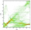 |
Fig. 1 Photometric redshifts estimated by HyperZ for a simulated flat distribution of galaxies. The colour scale shows the density of points, from black to yellow. |
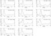 |
Fig. 2 Over-densities in the photometric redshift distribution for each cluster. In each panel the vertical line shows the spectroscopic redshift of the cluster. The plot represents the redshift distribution of the central area defined as R< 5′ minus the distribution of an annulus of same area starting at R = 10′. |
HyperZ can be very efficient with a sufficient number of photometric bands, but in this work we only have magnitudes in four filters with different limiting magnitudes, which makes it quite challenging to perform good photometric redshifts in all redshift ranges. Therefore we did not try to assign a photometric redshift to each individual galaxy and mainly focused on selecting cluster members and detecting the cluster over-density. To have a more quantitative estimate of the reliability of these photometric redshifts, we simulated a photometric catalogue with similar properties as our present observations. For simplicity, we used a flat redshift distribution, which is sufficient to test our redshift ranges of interest. We generated simulated magnitudes for 100 000 galaxies in the four MegaCam filters by adding noise according to the average signal-to-noise ratio (S/N) observed in our data. Then we ran HyperZ on this simulated catalogue and compared the photometric redshifts to the expected values (Fig. 1). Because of several colour−colour degeneracies, the reliability of HyperZ is not constant across the whole redshift range, and many high-redshifts galaxies with ztrue> 1.5 have an under-estimated photometric redshift zphot ~ 0.5. But for galaxies with 0.4 <ztrue< 0.6, the results are quite satisfactory: most of the galaxies have a photometric redshift as expected (±0.1), and only a small fraction of them have strongly deviating values. Therefore, we consider that the photometric redshifts estimated by HyperZ can be safely used to pre-select cluster members. A consistency check was made by considering the cluster over-density of galaxies: we determined the redshift distribution far from the cluster centre and subtracted it from the distribution obtained in a central region that covered the same area. The resulting redshift distribution clearly shows a peak located close to the cluster spectroscopic redshift (Fig. 2).
Global properties of the cluster sample.
2.4. Cluster colour−magnitude diagram
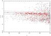 |
Fig. 3 Colour−magnitude diagram in the field of MS 1621.5+2640. The black points are the galaxies located at r< 500′′ from the cluster centre. The red dots are galaxies with r< 200′′ and a zphot compatible with the cluster redshift. The straight line is the best fit to the red sequence and the dashed lines are the 3σ limits of the red sequence. At the cluster redshift (z = 0.43), the expected colour, computed with the synthetic evolutionary code of Bruzual & Charlot (2003), is r′−i′ = 0.77. |
Early-type galaxies form a homogeneous population whose spectral energy distribution is dominated by red and old stars. For a given redshift, these galaxies are distributed along a well-defined red sequence in a colour−magnitude diagram, and this sequence extends over several magnitudes with a small scatter (typically smaller than 0.1 mag). This characteristic has long been used as a powerful tool for detecting clusters of galaxies in large photometric surveys (Gladders & Yee 2000). In the present study we used the red sequence of the galaxies to clean the lensing catalogues from cluster members. To identify this red sequence, we followed the method described by Stott et al. (2009): we first selected a sub-sample of objects located in the central area of the images (R< 200″ from the cluster centre), and we only kept galaxies with a photometric redshift compatible with the cluster redshift. We then performed a linear fit of the red sequence with a 3σ clipping to analytically determine the colour−magnitude relation in the (r′,r′−i′) diagram (Fig. 3). On average, the dispersion σ around the red sequence is 0.07 ± 0.02. Finally, we excluded all the galaxies in the whole catalogue along this relation and within ± 3σ of the Gaussian fit. We also applied a magnitude cut 18 <mr< 23 because fainter galaxies are no longer dominated by cluster members, and it is of prime importance to keep the background density as hgih as possible for the weak-lensing analysis.
In summary, the background galaxy catalogues were built for the present work with the following rules: a magnitude cut 22 <r′< 26 and a colour cut outside the red sequence ± 3σ, up to r′ = 23. Thus, most of the cluster members were removed. We checked that the galaxies density profile of the remaining galaxies is flat, except very near the cluster centre, where some residual contamination remains (see Paper I). However, this has no strong effect on the global morphology of the clusters that is described in this paper. The values of the average background galaxy density are given in Table 1, before and after cleaning the catalogues.
3. Stellar light distribution
3.1. Selection of cluster galaxies and global cluster properties
As stated in Sect. 2, we specifically built galaxy cluster catalogues by selecting galaxies whose r′−i′ colour falls within ± 3σ of the cluster red sequence. We also limited the sample to galaxies brighter than 0.4 L⋆, that is, m⋆ + 1, to avoid too much contamination in the faint-magnitude bins. The m⋆ magnitude was computed for each cluster, assuming an absolute magnitude M⋆−5log h = −20.44 (Blanton et al. 2003) and adding the appropriate distance modulus, the k-correction for an early-type galaxy for each cluster and the galactic reddening correction. Adding an evolution correction in the luminosity of the elliptical galaxies would amount to ~0.65 mag. This would decrease the intrinsic luminosity at a given apparent magnitude by a factor 1.8 and would also change the magnitude cut in the galaxy catalogues and reduce the number of cluster galaxies. All in all, the expected change in the total luminosity of the clusters is a factor of 2 to 2.2. But it is highly uncertain because it strongly depends on the galaxy evolutionary scheme used in the modelling of the evolution correction, and it is generally not included in general cluster studies. To remain consistent with previous works (see Popesso et al. 2004; Bardeau et al. 2007 for example), we chose not to include it in the present work.
Morphological properties of the luminous component of the clusters.
The total luminosity of the clusters was measured by summing the luminosity of all galaxies in the red-sequence interval that are located inside the radius R200 estimated with the weak-lensing analysis (Paper I). A background correction to the total luminosity was included by removing an average luminosity measured in an annulus defined by 2R200<r< 3R200 for each cluster and scaled with the adequate area. This correction is rather small because the total cluster luminosity is dominated by bright early-type galaxies. Finally, a correction for the magnitude cut of the galaxy catalogues was added (Popesso et al. 2004). It was calculated as the integral of a Schechter function up to 0.4L⋆ and with a slope α = 1.25 (Blanton et al. 2003). A factor 1.6 was then included to obtain the total luminosity of the clusters (Table 2). We also computed the cluster optical richness N200 , which we define as the number of cluster galaxies within R200 after correction for the background (Hansen et al. 2005). All values are given in Table 2.
3.2. Morphology of the light distribution
There are many possibilities to map the light distribution in a galaxy cluster. They depend on the choice of the input catalogues and on the method used to derive a correct mapping (see Okabe et al. (2010), for example). In the present case, we generated the light map trying to take the ellipticity and orientation of each individual galaxy into account more accurately to build the cluster light distribution. In practice, we selected cluster galaxies with magnitudes 18 <mr< 23 and colours along the red sequence (± 3σ). An artificial image was created for each with the package Artdata in IRAF 5, with parameters extracted from the photometric catalogues of the cluster galaxies (position, magnitude, ellipticity ε, and position angle PA). The resulting image was then smoothed with a Gaussian kernel to generate the cluster light map. We fixed the FWHM of the kernel to 80′′, a size twice smaller than the smoothing scale of the dark matter mass map. The maps are displayed for each cluster together with the mass distributions (Figs. A.1 to A.11). The ellipticity ϵ = 1−b/a and PA of the cluster light were measured on a 2D fit of the isophotes with Ellipse. For each cluster we favoured the large-scale morphology and fitted isocontours that in some cases encompass several clumps, especially in clusters with complex structure. In most cases, this corresponds to a radius 100 to 150′′, that is, up to 1 Mpc at the cluster redshift (Table 3). Error bars on the elliptical parameters are typically estimated from the change of the parameters when the radius varies from 90 to 150′′.
3.3. Brightest cluster galaxy
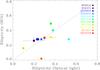 |
Fig. 4 Ellipticity of the global light distribution of the clusters versus the ellipticity of the brightest central galaxy. |
Brightest cluster galaxies are usually located at the very centre of clusters of galaxies. Numerous studies emphasized their specific properties compared to lower luminosity cluster members (Lin & Mohr 2004; Smith et al. 2010; Haarsma et al. 2010; Ascaso et al. 2011): luminosity, size and effective radius, star formation history and stellar populations, etc. It is still debated how best to distinguish the role of internal feedback processes, of the environment, and merging of satellite galaxies in the formation of the BCG. They also depend on the scenario of galaxy formation, and the ΛCDM paradigm seems to favour the importance of galaxy mergers at the centre of the main halo (De Lucia et al. 2007). In contrast, recent observations have confirmed the importance of baryonic feedback in the size evolution of the BCGs (Ascaso et al. 2011). It is beyond the scope of this paper to produce a detailed analysis of the structural parameters of the BCGs in our sample, and we simply compared their ellipticity and orientation (measured with Sextractor) with the large-scale light and dark matter distributions (Table 3). The link with the dark matter ellipticity is not obvious, but the correlation between the light distribution and the central BCG is quite convincing (Fig. 4), except for two outliers that have complex sub-structures. Quantitatively, we find a weighted mean ⟨ εlight−εBCG ⟩ = 0.001 ± 0.12, and the mean orthogonal deviation from the 1:1 line (εlight = εBCG) is 0.06. This value decreases to 0.03 if we remove the two major outliers and is then well below the uncertainties in the ellipticity measurements, of the order of 0.05. This result is not surprising as the alignment of the BCG with the distribution of galaxies at large scale was first observed by Lambas et al. (1988) and has been confirmed since then by many studies (Panko et al. 2009; Niederste-Ostholt et al. 2010).
In a second step, we separated the clusters into two classes: those dominated by a single giant elliptical galaxy, most often embedded in an extended envelope (a cD-type galaxy), and those for which more than one bright galaxy forms the cluster centre, or the brightest cluster member does not outshine other galaxies. Five out of 11 clusters are dominated by a cD galaxy, namely RXC J0856.1+3756, RX J1120.1+4318, RXC J1206.2–0848, MS 1241.5+1710, and RX J2228.5+2036. Surprisingly, they are not necessarily the brightest clusters in terms of total stellar luminosity, nor are they the most massive ones, suggesting that the formation of a giant cluster galaxy is not only related to the initial halo conditions, but also to the evolution processes in the clusters and the merging history of the structures (Dubinski 1998).
General properties of the weak-lensing mass maps for the cluster sample.
4. Bi-dimensional weak-lensing analysis and dark matter distribution
4.1. Mass reconstruction
We refer to Paper I for the details of the weak-lensing implementation. In summary, the galaxy shapes were measured with the Im2shape software (Bridle et al. 2002). For each object a parametric shape model was set up with an ellipse. Im2shape convolves this model with the local PSF and subtracts it to the sub-image centred on the galaxy. A Markov chain Monte Carlo (MCMC) minimizer applied on the image residuals provides the intrinsic shape parameters and error estimates. The point spread function (PSF) is measured directly on the images by averaging the shapes of the five stars closest to each galaxy. All measures were made on the r′ images, which were obtained with the highest image quality. Only galaxies for which the measured ellipticity error was smaller than 0.25 were kept in the working catalogues. The main results for the mass measurements and the study of the global properties of the clusters are presented in Paper I, as is a careful analysis of the sources of error in the mass determination. In the present work, we focus on the spatial distribution of the dark matter traced by the weak-lensing map reconstruction.
We used the software LensEnt2 kindly provided by P. Marshall (Marshall et al. 2002) to build the weak-lensing mass maps. The method is based on an entropy-regularized maximum-likelihood technique. It uses the shape of each background galaxy as an individual estimator of the local reduced shear. The pixel size on the mass grid is chosen to have approximately one galaxy per pixel, which leads to a similar number of data and free parameters. To consider the fact that clusters have an extended and smooth mass distribution, the code includes a smoothing via the size of the intrinsic correlation function (ICF): the physical mass map is expressed as a convolution of the “hidden” distribution (the pixel grid) with a broad kernel defined by the ICF. The shape and size of this ICF are the main control parameters of LensEnt2 and reflect the spatial resolution of the reconstructed mass map. For simplicity, we only used a Gaussian ICF with a width of 150′′ for all clusters. This represents a good compromise between smoothness and details in the mass map. LensEnt2 also computes error maps that locally give the width of the probability function in the mass reconstruction. The average value of the error map within the central area of the CCD image (15′ × 15′) is a good estimate of the level of uncertainty in the mass reconstruction. This value determines the S/N of the detected peaks (Table 4).
LensEnt2 provides output mass maps in physical units of surface mass density (M⊙ pc-2). This is valid provided that the redshift distribution of the background sources is well known. In the present case, we worked with source catalogues that were cleaned for galaxy cluster members, but still contaminated by foreground galaxies. A rough estimate of this contamination comes from the redshift distribution of galaxies in the magnitude range selected for our catalogue: if we apply the same selection criteria on the deep photometric catalogue with photometric redshifts built from the CFHTLS-Deep survey (Coupon et al. 2009), we find that about 25% of the galaxies are at a redshift lower than 0.5, that is, foreground galaxies. This is coherent with the number found in deep spectroscopic surveys, although at slightly brighter magnitudes (Le Fèvre et al. 2005). In our case, the effect of this uniform contamination is mostly a dilution of the weak-lensing signal, which means that the output mass densities of LensEnt2 are not reliable in their absolute values. Moreover, there remains some additional contamination from cluster galaxies in the very centre of the clusters (see Fig. 3 in Paper I). The main effect is to attenuate the peak intensity and to decrease the S/N ratio of the cluster component. But we do not expect any significant influence on the shape of the mass reconstruction, provided the contaminating cluster members are randomly oriented within the cluster. This assumption is valid in our case because the galaxy catalogues include cuts in colour and magnitude that eliminate all bright cluster members. The remaining galaxies are mostly blue and/or faint and therefore are less sensitive to intrinsic alignment effects (Mandelbaum et al. 2011). In the rest of the paper we therefore concentrate our work on the 2D mass distribution. The mass map reconstructions are displayed for each cluster in the Appendix.
4.2. Ellipticity of the mass distribution
The ellipticity of the mass distribution traced by the weak-lensing mass reconstruction has been the focus of several studies. It is direct evidence of the triaxiality of the cluster halos and is expected to be a non-negligible factor in the growth of massive halos in the ΛCDM paradigm (Limousin et al. 2013). Oguri et al. (2010) studied a sample of 25 massive X-ray clusters (mostly in the LOCUSS sample) at redshift ~0.2. They found an average ellipticity ⟨ϵ⟩ = 1−b/a = 0.46 ± 0.04. More recently, Oguri et al. (2012) confirmed the trend with another independent sample of clusters built from the Sloan Giant Arcs Surveys as part of the SDSS (Hennawi et al. 2008). These values of the mean ellipticity agree well with the theoretical predictions based on numerical simulations of cluster dark matter halos (Jing & Suto 2002). They correspond to what is expected for massive clusters, in contrast to low-mass clusters, which are expected to be more circular.
We tried to explore this question with the present sample. But because our sample is at higher redshift than LOCUSS, several difficulties limit the outcomes of the approach. To estimate the uncertainties of the elliptical parameters for each mass reconstruction, we used a jackknife resampling method to remove 10% of the galaxies in the source catalogue and repeated the process ten times. The removed galaxies all differ from one attempt to the next. Ten new mass maps were computed for each cluster with these sub-catalogues, as well as the corresponding error maps. The ten error maps were averaged, and the average level of this frame gives the 1σ level of the mass reconstructions. We then fitted each of the ten mass maps with elliptical contours and selected the elliptical parameters of the 3σ isocontour. An average of the ten fits gives the final values for the elliptical parameters (ε and PA) and their standard deviation (Table 4). This process was acceptable except for the clusters RX J1120.1+4318 and MS 1241.5+1710, which have the lowest S/N maps. We restricted their fits to the 2σ and 2.5σ isocontours, respectively.
In all cases this corresponds to an isocontour of 100 to 150′′ in radius (or 600 to 900  kpc at redshift 0.5). But because of the limited resolution of the mass reconstruction, the effect of the central smoothing by the ICF is quite significant and induces an attenuation in the measure of the mass ellipticity. In practice, an ICF of 150′′ corresponds to a Gaussian smoothing with σ ~ 60″. As a test case, we simulated a set of mass maps with multiple clumps of matter and tested the effects of the smoothing on the ellipticity of the mass distribution. In practice, each clump was generated with a Navarro-Frenk-White (NFW) profile with c = 4 and
 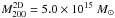 (associated with rs = 60″ = 360 kpc, r200 = 1.4 Mpc, and M200 = 3.9 × 10¹⁴M⊙). Three clumps were aligned along a line and regularly spaced, with separations ranging from 40′′, 60′′ and 80′′ (250 kpc to 500 kpc at z ~ 0.5) between the clumps. The 2D mass maps were then smoothed with two different kernels, with σ = 30″ and σ = 60″, corresponding to an ICF of 75′′ and 150′′ in the mass reconstruction. The ellipticity of the simulated mass distributions was measured with the same method as for the clusters maps, with the centering fixed on the central mass peak, for both the smoothed and unsmoothed distributions (Fig. 5). The relevant ellipticiy was measured in radii between 100′′ and 150′′ for the observed clusters. The measures on the simulated clusters show that the apparent ellipticity is typically decreased by a factor 2 when applying this severe smoothing. We did not attempt to correct for the measured ellipticities more accurately because the ellipticity attenuation probably also depends on the mass profile, which is not well enough constrained in this study. A higher background galaxy density would have allowed sharper mass reconstructions, but this is beyond reach with ground-based wide-field imaging and requires data that have the quality of those the HST provides.
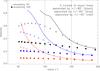 |
Fig. 5 Ellipticity of simulated clusters formed by 3 mass clumps with NFW profile, and smoothed with 2 different kernels. The continuum line is the ellipticity measured on the unsmoothed data. For comparison the ellipticity of the observed clusters was measured in radii ranging from 100 to 150′′ approximately. |
The results of the elliptical fitting of the cluster mass distribution are presented in Table 4. Half of the clusters have a low ellipticity (five clusters with εDM< 0.2), while the other half is clearly elliptical (six clusters with εDM> 0.2). The ellipticity distribution of the sample shows a weighted mean of ⟨ϵ⟩ = 0.25 ± 0.12. It appears to be narrower than that of other samples like LOCUSS (Oguri et al. 2010). But we have fewer clusters, and it is more difficult to provide weak-lensing maps at redshift 0.5. No value exceeds 0.40, in contrast to what is expected for such a cluster sample, and none of the clusters is really circular (εDM< 0.1) in their extended regions. The smoothing process, needed to derive an acceptable mass map at high redshift, is certainly the cause of the lack of high ellipticity clusters in our sample (Fig. 5). In conclusion, even if we cannot draw firm conclusions on the ellipticity distribution of the dark matter from our sample, we show that we remain compatible with standard expectations and previous works. A similar attempt to test the evolution of the ellipticity of the X-ray gas distribution was proposed by Maughan et al. (2008) with Chandra data. They did not find any change in the ellipticity distribution of the high-z sample (>0.5) compared to their low-z sample, in contrast to other morphological parameters like the slope of the surface brightness profile at large radius.
We also compared the distance between the main mass peak and the location of the BCG to check the consistency between the positions of the dark matter peak and the light peak. However, the uncertainty in the centring of the mass distribution is high and strongly depends on the S/N ratio of the main mass peak. As demonstrated with numerical simulations by Dietrich et al. (2012), the shape noise in the weak-lensing map reconstruction combined with the smoothing process generates an offset distribution with a mode as large as 0.3′ and median values up to 1′ for typical ground-based observations. In our case, the clusters with the best map reconstruction and the highest S/N in the central peak (>5) are also those for which the position of the mass peak matches the position of the BCG as well as the centroid of the gas distribution (Figs. A.1 to A.11). This is generally valid, except for the clusters RX J0943.0+4659 (merging cluster) and MS 0015.9+1609. This last cluster deserves some comment because previous weak-lensing modeling of the central area, using HST/ACS images, point towards a mass centre that is well centered on the three brightest galaxies (Zitrin et al. 2011). Our mass reconstruction suffers from the proximity with a bright star and its halo, which distorts the shape distribution of the faint galaxies.
More interesting is the distribution of the X-ray/BCG offset. It clearly appears to be bi-modal, with most of the clusters having an offset smaller than 50 kpc, and three outliers. Among these three clusters, two are merger systems, and the last one, RX J1120.1+4318 is rather poorly defined in its centre. This is a similar trend as was found by Sanderson et al. (2009) in the LOCUSS sample of low-redshift clusters. This X-ray/BCG offset is a good indicator of the dynamical state of the cluster and is highly correlated with the strength of the cooling core in the centre. The comparison between the X-ray and the mass peaks is more uncertain because of the limitations mentioned above. But it shows a similar trend, at least for the clusters with a mass peak detected with a high enough significance.
5. Mass and light distributions
5.1. Comparison between light and mass 2D distributions
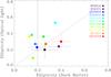 |
Fig. 6 Ellipticity of the optical light distribution versus the ellipticity of the dark matter. The vertical line separates the cluster sample between the circular clusters with ϵ< 0.2 and the elliptical or irregular clusters. |
Figure 6 shows the correlation between the ellipticity of the dark matter and that of the stellar light distributions. As for the comparison between the cluster light and the BCG ellipticities, we measured a weighted mean ⟨ εDM−εlight ⟩ = −0.1 ± 0.02 and the mean orthogonal deviation to the εDM = εlight line is 0.08 for the 11 clusters. Dispersion is slightly higher than for the light-BCG comparison, but again we find a good concordance between the two ellipticities and a tendency towards a better agreement for elliptical clusters than for circular ones. We recall that these measurements correspond to large-scale morphologies, which means that they are more sensitive to substructures that can be found at the Mpc scale. Weak-lensing morphology can also be disturbed by additional mass halos that are projected on the line of sight, but are not physically related to the clusters. Similar conclusions were reached by Oguri et al. (2010) from a very similar study.
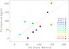 |
Fig. 7 Orientation of the optical light distribution versus the dark matter. The circular clusters with an ellipticity ϵ< 0.2 are marked with a cross. |
To study the possible alignment effect between the light and the dark matter distributions, we represented the position angle of the optical light versus the position angle of the dark matter distribution (Fig. 7). To better visualize the shift with respect to the y = x line, we also computed the distance between the data points associated with the clusters and the 1:1 line in that plane. The position angles of the two distributions are strongly correlated: the mean difference ⟨ ΔPA ⟩ = ⟨ PA(DM)–PA(light) ⟩ = + 3 ± 3° degrees and the average deviation to the 1:1 line is 28°. In addition, as shown in Fig. 8, these differences tend to vanish when the ellipticity increases. We suspect that large differences at small ellipticities are partly due to biases in the processing of the elliptical fits or to the influence of further substructures at large radius. However, Oguri et al. (2010) showed in their detailed study that elliptical fits of weak-lensing maps are robust when they use similar radii of 400 to 800 kpc. We are therefore confident that in the present study the “light traces mass” assumption is valid when clusters are in quiescent phases of their evolution. Departures from this assumption occur when the clusters enter merging processes and when interactions between large clumps of matter globally perturb their dynamical equilibrium.
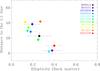 |
Fig. 8 Orthogonal deviation (in degrees) from the 1:1 line for the dark matter orientation (PA(DM)) compared to the light distribution orientation (PA(light)) versus the ellipticity of the dark matter distribution. The more elliptical this distribution, the better the alignment between light and dark matter. |
5.2. Cluster mass-to-light ratio
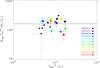 |
Fig. 9 Mass-to-light ratio versus the total luminosity |

The mass-to-light ratio is a quantity that has been widely studied at every mass scale, from single galaxies up to rich and massive galaxy clusters. Its variation across the mass range for instance allows highlighting physical processes that affect the baryonic component of massive structures, such as star formation or galaxy-galaxy interactions in large dark matter halos (Carlberg et al. 1996; Marinoni & Hudson 2002; Giodini et al. 2009). In Paper I, we analysed the correlation between mass and luminosity and found a logarithmic slope of 0.95 ± 0.37 for the mass-luminosity scaling law, compatible with a constant M/L ratio. In the present paper, we used the 2D projected mass  instead of the 3D mass used in Paper I. These two masses mostly differ by a scale factor because all clusters are assumed to have the same concentration parameter. This projected mass is the correct quantity to be compared to the total projected luminosity. We therefore correlated the 2D mass with the total luminosity of early-type galaxies, computed inside the radius R200 and corrected from the non-detected part of the luminosity function. We obtain an average ratio ⟨M/L⟩ = 160 ± 60 h70 (M/L)⊙, with values ranging from ~68 to 235 (Table 2 and Fig. 9). Our results agree excellently well with the values obtained by Bardeau et al. (2007), who used a similar methodology to derive the weak-lensing masses and the optical luminosities for a sample of clusters at lower redshifts (z ~ 0.2). They found an average ratio of ⟨M/L⟩ = 170 ± 67 for the same quantities, and their results are very similar to ours. Because the methodology they used is so close to ours, we merged the two samples, even though the clusters differ in redshift. From the 22 clusters we find an average ratio ⟨M/L⟩ = 166 ± 62 h70 (M/L)⊙. Comparisons with other samples are rather difficult because several methodologies were used to derive optical luminosities (Popesso et al. 2007), and we cannot discuss further here.
In addition, although the mass interval of the sample is rather limited, ranging from 6 × 10¹⁴M⊙ to 2.5 × 10¹⁵M⊙, we tried to consider the possible variation of the M/L ratio with mass. This is rather speculative and limited by the fact that the clusters with the lowest mass are also those with the largest uncertainty in the weak-lensing peak detection and because the two quantities are correlated. Following the same procedure as described in Foëx et al. (2012), we fitted the M versus L relation using a linear regression in the log–log plan with the orthogonal BCES method, which takes into account errors in both directions and provides a statistical dispersion around the fit σstat as well as the intrinsic dispersion σ−int. We did not find any significant departure from a constant ratio between the two quantities, with a slope α = 0.945 ± 0.37,σint = 0.14 and σstat = 0.11 for the dispersions of the fit in the log–log space. With the present data we do not find any departure from a constant M/L ratio independent of the total cluster mass, although previous works have found a significant increase of the M/L ratio for massive clusters of galaxies compared to lower mass clusters and groups (Popesso et al. 2007; Andreon 2010). But this was obtained with samples spanning a much broader mass interval than ours. The physical origin of this situation is still controversial, but it is usually understood in terms of a decrease of the star formation efficiency with increasing halo mass (Springel & Hernquist 2003; Lin et al. 2003).
6. Summary and conclusions
The cluster sample we presented is limited to only 11 clusters, at a redshift z ~ 0.5. They were selected according to their X-ray emission and are part of the representative sample EXCPRES, which includes 20 clusters in the redshift range 0.4 <z< 0.6. Because of additional criteria used to optimize the weak-lensing detection and analysis, our sample is not any more representative of the cluster population at intermediate redshift, but it forms a sub-sample with the brightest X-ray luminosity. We summarize below the properties of the clusters we explored:
-
We provided for each cluster the total luminosity after a carefulidentification of cluster members. We also listed severalmorphological parameters of the light distribution. We find goodcorrelations between the ellipticity of the BCG and the globallight distribution in terms of ellipticity and orientation. Butregardless of whether the BCG has a bright and extendedenvelope of cD-type or not, there are no significant differences inthe general optical properties of the clusters.
-
The weak-lensing mass reconstruction was made for each cluster, although the peak detection was at low significance in a few cases (one cluster detected at less than 3σ). The average ellipticity of the mass maps is ⟨ ϵ ⟩ = 0.25, which is compatible with similar estimates at lower redshift. No evolution of the average ellipticity of the clusters or the fraction of high-ellipticity mass distributions is detectable in our data. We also explored the distance between the mass peak, the location of the BCG, and the X-ray centre for each cluster. The position of the mass peak is the most uncertain and is limited intrinsically by the low density of background galaxies in the mass reconstruction. In contrast, we find good agreement between the location of the BCG and the X-ray centre, especially for regular clusters. As expected, the most discrepant clusters are those with the most disturbed morphology or clear signs of dynamical perturbations.
-
The mass-to-light ratio distribution agrees excellently well with previous measurements made with a similar approach, and we found an average M/L ratio of ⟨M/L⟩ = 160 ± 60 h70 (M/L)⊙. Previous studies were made at lower redshift, and we do not find a significant sign of evolution, as expected for this intermediate-redshift bin.
These properties point towards a general picture of the clusters that is mainly driven by the paradigm “the light follows mass” . This good agreement is valid both in the central parts of the clusters and at large scale, as demonstrated with the weak-lensing mass reconstructions. At greater detail, we tried some attempts to separate the sample in two classes, as was done previously for other cluster samples such as LOCUSS or the CCCP (Smith et al. 2005; Mahdavi et al. 2013). A majority of clusters are regular and follow the main correlations, and three or four outliers are identified as unrelaxed clusters or merger systems (namely RX J0943.0+4659, RXC J1003.0+3254, RX J2228.5+2036, and possibly MS 1241.5+1710). To better quantify departures from the assumption of regularity, it will be important to study and better understand the influence of substructures and the role of triaxiality. It is a natural consequence of structure growth driven by self-gravity of Gaussian density fluctuations (Limousin et al. 2013), but up to now, it has mostly been neglected, for simplicity. We now have gained a good understanding of the tracers of the distribution of the different components in clusters, therefore it is timely and appropriate to address this issue in detail. This would allow improving mass measurements and the understanding of the mass growth of structures, such as massive as clusters of galaxies.
Online material
Appendix A: Individual cluster properties
The 11 clusters presented in the sample are all bright X-ray clusters. Some of them also present specific optical properties or are already known as strong gravitational lenses. We review in this section the properties of the clusters, mostly in the optical. Their X-ray properties will be presented in a companion paper (Arnaud et al., in prep.).
Appendix A.1: MS 0015.9+1609 (z = 0.541)
This very rich cluster has been studied for many years, since the identification of a high fraction of red galaxies in its population (Koo 1981). Included in the CNOC cluster sample, its spectroscopic survey was presented in Ellingson et al. (1998) with more than 180 objects observed spectroscopically. The resulting velocity dispersion  km s-1 is a high value consistent with its galaxy richness (Borgani et al. 1999). MS 0015.9+1609 is one of the brightest and most distant X-ray cluster included in the EMSS sample (Gioia & Luppino 1994). It is also part of the highly luminous X-ray clusters identified in the MACS sample at redshift higher than 0.5 (Ebeling et al. 2007) and is identified as MACS J0018.5+1626.
The weak-lensing properties were described by Smail et al. (1995) and then by Clowe et al. (2000). The authors found a rather low signal and therefore a total mass not consistent with the optical velocity dispersion of the galaxies. More recently, Hoekstra (2007) re-analysed a large sample of clusters observed in good seeing conditions at the CFHT and found for MS 0015.9+1609 a total mass described by a SIS with  km s-1 or by a NFW profile with
  . Note that despite the high mass value of the cluster, no strong-lensing features were detected in HST images (Sand et al. 2005). More recently and thanks to a detailed analysis of HST/ACS images, Zitrin et al. (2011) identified three systems of multiple images, but they have not yet been confirmed spectroscopically. They were used to provide a lensing model of the mass distribution in the centre of the cluster.
There is no dominant central galaxy in this cluster but a chain of bright ellipticals, giving a significant elongation in the galaxy distribution. This elongation was confirmed in the weak-lensing map provided by Zitrin et al. (2011) on the central area of the cluster. In our wide-field map, the ellipticity of the mass distribution does not appear clearly (Fig. A.1). We suspect that the bright star close to the cluster centre prevents a correct study of the cluster mass map obtained from weak-lensing reconstruction.
MS 0015.9+1609 is embedded in a large-scale structure of the size of a supercluster, identified spectroscopically by Connolly et al. (1996). At least three clusters lie within less than 30 Mpc form each other, and a long and massive filamentary structure crosses the cluster in the same direction as the galaxy elongation (Tanaka et al. 2007, 2009). The weak-lensing reconstruction we presented only focused on the central area around the cluster, but we checked that most of the structures spectroscopically identified by Tanaka et al. (2007) were also visible in our global mass map. This may be the case for the south-west elongation seen in the mass map displayed in Fig. A.1. Further work is in progress to better quantify these correlations.
Appendix A.2: MS 0451.6–0305 (z = 0.537)
This cluster is the most X-ray luminous cluster in the EMSS catalogue (Gioia & Luppino 1994) and is also part of the CNOC sample. Intensive spectroscopic follow-up of the galaxies provided more than 100 spectra of cluster members (Ellingson et al. 1998) and a line-of-sight velocity dispersion of  km s-1 (Borgani et al. 1999). Weak-lensing masses measured by Clowe et al. (2000) are roughly compatible with this value as well as those obtained by Hoekstra et al. (2012). Our own measurements are higher by 50%, but they remain compatible within the uncertainties (Foëx et al. 2012). The cluster is also identified as MACS J0454.1–0300.
A few thin and elongated features were suspected to be strong-lensing candidates by Luppino et al. (1999) and were later spectroscopically confirmed by Borys et al. (2004). Interestingly, a SCUBA detection of an extended source in the cluster centre led to the identification of an ERO pair, triple imaged (Chapman et al. 2002; Takata et al. 2003; Berciano Alba et al. 2010). These features point towards the bright central galaxy as the centre of the mass distribution. The observed elongation of the weak-lensing mass reconstruction (Fig. A.2) is well correlated with the global elongation of the light distribution in the SE/NW direction. This is also true for the orientation of the BCG. The latest strong-lens model presented by Zitrin et al. (2011) indicates that the central mass distribution is highly elliptical, with an orientation that matches the SE/NW elongation of the cluster at large scale.
Appendix A.3: RXC J0856.1+3756 (z = 0.411)
This cluster is part of the NORAS sample (Northern ROSAT all-sky galaxy cluster survey), a purely X-ray selected sample (Böhringer et al. 2000). It was included in the EXCPRES sample because of its high X-ray luminosity. It is an optically bright cluster identified in the SDSS-DR6 ([WHL2009] J085612.7+375615, Wen et al. 2009), with a redshift measurement of the BCG at z = 0.411. The cluster displays a well-defined and regular luminous over-density dominated by a bright and extended cD galaxy (Fig. A.3). The mass map also presents a very regular aspect around its centre and provides a coherent picture of a relaxed cluster.
Appendix A.4: RX J0943.0+4659 (z = 0.407)
This cluster is also known as Abell 851 or Cl 0939+4713. It is the only Abell cluster of our sample. High-resolution HST images of the centre revealed a large population of blue galaxies and many merging galaxies (Dressler et al. 1994). Seitz et al. (1996) used this deep HST/WFPC2 image to identify a few lensed objects, but no highly magnified gravitational arcs were detected. X-ray observations of A851, first with ROSAT and more recently with XMM-Newton, showed a very perturbed distribution with pronounced substructures and evidence for a dynamically young cluster (De Filippis et al. 2003). Tentative 2D spectro-imaging led to the identification of a hot region between the two main sub-clusters, a characteristic of a major merger in an early phase.
The galaxy distribution is complex, with a high galaxy density in the central area. It can be separated into two clumps that trace the cluster interaction and are coherent with the gas distribution. Several bright galaxies dominate the light distribution and are more concentrated in the south-west extension of the cluster (Fig. A.4). In contrast, the weak-lensing mass map is surprisingly regular, with only one main structure, but elongated along the direction of the interaction. The separation between the two X-ray peaks is 50′′, well below the resolution of the mass map. With the present data there is therefore no chance to obtain a more detailed view of the mass distribution at a scale where the physical processes of the cluster merger could be identified. Deeper imaging is necessary to proceed in this analysis. Because of the high evidence for merging processes, this cluster was later removed from the EXCPRES sample, but as optical data were obtained in good conditions, we kept it in our sample.
Appendix A.5: RXC J1003.0+3254 (z = 0.416)
The cluster was initially identified by its X-ray extended emission in the NORAS sample (Böhringer et al. 2000), and it was later re-detected in the 400d ROSAT sample (Burenin et al. 2007). Nothing was really known on the optical properties of this cluster, which displays a bright galaxy in its centre and a rather loose distribution of cluster members. Another bright galaxy is located 2.3′ south-west, with similar properties. It is centred on a secondary peak in the X-ray gas distribution and the mass map is centred in between these two galaxies. But the bi-modality of the cluster is more visible in the galaxy distribution than in the mass map (Fig. A.5), which is limited by its spatial resolution. We suspect that this cluster results from the merging of two sub-clusters, and all conclusions regarding RXC J1003.0+3254 in the global analysis of the sample must be taken with caution.
Appendix A.6: RX J1120.1+4318 (z = 0.612)
This cluster belongs to the Bright SHARC survey (Romer et al. 2000) and was included in the WARPS II catalogue (the Wide Angle ROSAT Pointed Survey, Horner et al. 2008). The cluster was observed with XMM-Newton and analysed by Arnaud et al. (2002), who found a regular X-ray emission with a spherical morphology. They also claimed that no cooling flow or central gas concentration is present in this cluster, which is consistent with the cooling time being longer than the age of the Universe at this redshift. With its redshift z = 0.612, RX J1120.1+4318 is the most distant cluster of the EXCPRES sample. The light distribution of cluster members shows an east-west elongation, which was also been measured in the Chandra X-ray map (Maughan et al. 2008). But the ellipticity is rather low and does not attenuate the regular morphology of the cluster, which is clearly in a relaxed phase. Unfortunately, the lensing signal in RX J1120.1+4318 is barely detected, at less than 3σ (Fig. A.6). This makes it difficult to draw any conclusions on the mass distribution in the cluster. Even the shift between the mass peak and the light peak cannot be considered significant.
Appendix A.7: RXC J1206.2–0848 ((z = 0.441)
This cluster is one of the brightest clusters of the REFLEX sample (Böhringer et al. 2004). It belongs to the MACS sample (Ebeling et al. 2010) as MACS J1206.2–0847 and is part of the CLASH sample (Postman et al. 2012). It displays a bright and spectacular arc system, initially spectroscopically observed by Sand et al. (2004) and confirmed more recently by Ebeling et al. (2009) at a redshift z = 1.036. A detailed analysis of the central mass distribution was made both with strong-lensing and X-ray data, giving a discrepancy of a factor 2 between the two mass estimates. But the X-ray distribution of the gas shows some signs of merging processes in the centre, which could explain this discrepancy. Similar trends have already been noticed in other clusters such as A1689 (Limousin et al. 2007).
The weak-lensing mass distribution is clearly peaked, with a regular shape and a central concentration that fits the luminous mass as well as the X-ray mass (Fig. A.7). Note that the central galaxy is also a bright radio source with a steep spectrum (Ebeling et al. 2010).
Umetsu et al. (2012) recently comprehensively analysed this cluster by combining weak and strong lensing derived from wide-field Subaru imaging and HST observations. Their morphological analysis of both the reconstructed mass map and light distribution revealed the presence of a large-scale structure around RXC J1206.2–0848. The orientation of this structure matches the position angle of the BCG and that of the cluster light distribution and projected mass map. The ellipticity they derived for the latter is somehow higher than ours, but we obtain consistent results for the light distribution. The overall shape of RXC J1206.2–0848 indicates that light follows mass up to the large scales of the cosmic web.
Appendix A.8: MS 1241.5+1710 (z = 0.549)
As part of the EMMS sample (Gioia & Luppino 1994), this cluster was also observed in the optical, but no significant strong-lensing feature was detected (Luppino et al. 1999). The luminosity distribution is complex, with a southern extension possibly related to the main cluster. However, neither the mass distribution nor the X-ray gas shows a similar trend. Both are regular and centred in the BCG, embedded in a bright and extended envelope. This means that firm conclusions are difficult to draw because of the low S/N ratio of the mass map (Fig. A.8). The second over-density of galaxies could also be due to some contamination along the line of sight. Deeper and multi-colour images are necessary to confirm the reality of an in-falling substructure on the main cluster.
Appendix A.9: RX J1347.5–1145 (z = 0.451)
This is the brightest cluster of the REFLEX sample (Böhringer et al. 2004) and is part of the CLASH sample (Postman et al. 2012). It presents the spectacular strong-lensing system detected by Schindler et al. (1995). It was also identified as a cluster with a strong central cooling flow (Allen 2000), feeding a powerful radio source (Pointecouteau et al. 2001). A detailed combined analysis of the strong- and weak-lensing effects (Bradač et al. 2005a,b) led to a very accurate view of the dynamical status of the cluster in the inner regions: the cluster presents a mass concentration centred on the BCG with some extension to the SW and much evidence of sub-cluster merging. But RX J1347.5–1145 is definitely not a major merger. After some controversy, the different mass estimates seemed to converge, especially those measured close to the centre using the strong-lensing features (Halkola et al. 2008; Bradač et al. 2008). But a factor of 2 remains between the X-ray and the weak-lensing masses at large radius (Fischer & Tyson 1997; Kling et al. 2005; Gitti et al. 2007). In this context, our mass map confirms the previous results and does not bring new evidence on the mass distribution (Fig. A.9). It was mostly used to check and validate our weak-lensing procedure before applying it to other clusters. Similar results were published on RX J1347.5–1145 by Hoekstra et al. (2012) with the same CFHT data. Fortunately, they obtained very similar mass measures.
Several studies (Lu et al. 2010; Verdugo et al. 2012) revealed that RX J1347.5–1145 is embedded in a large-scale structure, extending up to 20 Mpc in the NE–SW direction. Our luminosity map confirms the existence of several over-densities on a large scale, aligned along this direction. The main orientation of the cluster light distribution also follows the same direction. Like RXC J1206.2–0848, this cluster supports the picture of the cosmic web where massive clusters are fed by filaments whose orientation matches the global morphology of the central node.
Appendix A.10: MS 1621.5+2640 (z = 0.426)
As part of the EMSS cluster sample (Gioia & Luppino 1994), the cluster was rapidly identified as a strong lens with a nice gravitational arc located around a radio galaxy that is not the brightest cluster galaxy (Luppino et al. 1999). No spectroscopic redshift is currently available for the arc, although its lensed nature is not in doubt (Sand et al. 2005). MS 1621.5+2640 is also part of the CNOC sample and was spectroscopically observed with more than 100 cluster redshifts available (Ellingson et al. 1997). The velocity dispersion is low ( km s-1, Borgani et al. 1999). More recently, Hoekstra (2007) reported a very accurate weak-lensing analysis, and his results agree well with the dynamical mass estimate. It is also consistent with the X-ray mass obtained with ROSAT (Hicks et al. 2006). With our weak-lensing mass reconstruction, we find a mass distribution rather elongated and coherent with the light distribution. The large shift between the mass and light peaks is more probably an artefact than real (Fig. A.10).
Appendix A.11: RX J2228.5+2036 (z = 0.412)
This cluster is part of the NORAS sample (Böhringer et al. 2000) and also belongs to the MACS sample (MACS J2228.5+2036, Ebeling et al. 2007). Because it is at low galactic latitude, very few optical observations are available. Our weak-lensing reconstruction is rather uncertain (Fig. A.11) and possibly flawed because of the large number of bright stars in the field of view. However, in addition to its strong X-ray emission, this cluster was detected for its SZ signal, allowing one of the first combined analyses between the X-ray and the SZ signals (Pointecouteau et al. 2002; Jia et al. 2008). Both confirm that the cluster is quite massive and dynamically perturbed. The weak-lensing map shows a poor signal close to the cluster centre but suggests that the cluster has an elongated shape. This is also valid for the complex light distribution. The most convincing feature is a galaxy clump located in the south-west direction, detected on the mass map with higher significance than the main cluster. It is associated with a galaxy excess centred on a bright elliptical galaxy with similar magnitude as the cluster BCG. We suspect that this clump is at a similar redshift as RX J2228.5+2036 and may be the cause of a future major merger with RX J2228.5+2036. Surprisingly, there is no X-ray counter-part to this clump.
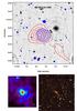 |
Fig. A.1 Up: 15′ × 15′ inset of the cluster field extracted from the full r′ MegaCam image. The thick red contours show the mass distribution derived from the 2D weak-lensing analysis. The contour levels are linearly spaced in σ of the mass reconstruction, starting at 2σ. The thin blue contours come from the X-ray map obtained with XMM-Newton. The image was filtered with wavelets and the contours are scaled logarithmically. Bottom left: same mass isocontours overlaid on the galaxy luminosity distribution where cluster members are selected within the cluster red sequence and mr< 23. Bottom right: true colour image of the cluster centre from g′, r′, i′ combination. The field of view is 3′ × 3′. |
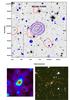 |
Fig. A.2 Same as Fig. A.1, for MS 0451.6-0305. |
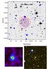 |
Fig. A.3 Same as Fig. A.1, for RXC J0856.1+3756. |
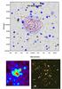 |
Fig. A.4 Same as Fig. A.1, for RX J0943.0+4659. |
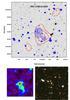 |
Fig. A.5 Same as Fig. A.1, for RXC J1003.0+3254. |
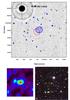 |
Fig. A.6 Same as Fig. A.1, for RX J1120.1+4318. |
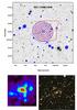 |
Fig. A.7 Same as Fig. A.1, for RXC J1206.2-0848. |
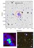 |
Fig. A.8 Same as Fig. A.1, for MS 1241.5+1710. |
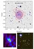 |
Fig. A.9 Same as Fig. A.1, for RX J1347.5-1145. |
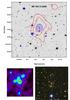 |
Fig. A.10 Same as Fig. A.1, for MS 1621.5+2640. |
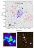 |
Fig. A.11 Same as Fig. A.1, for RX J2228.5+2036. |
Acknowledgments
We thank Gabriel Pratt, Marc Huertas, and Roser Pello for fruitful discussions and encouragements. We acknowledge support from the CNRS/INSU via the Programme National de Cosmologie et Galaxies (PNCG). E.P. and G.S. acknowledge the support of ANR under grant ANR-11–BD56-015. G.F. acknowledges support from FONDECYT through grant 3120160. M.L. acknowledges supports from the CNRS and the Dark Cosmology Centre, funded by the Danish National Research Foundation. The present work is based on observations obtained with XMM-Newton, an ESA science mission with instruments and contributions directly funded by ESA Member States and the USA (NASA), and on data products produced at Terapix and the Canadian Astronomy Data Centre. The authors wish to recognize and acknowledge the very significant cultural role and reverence that the summit of Mauna Kea has always had within the indigenous Hawaiian community. We are most fortunate to have the opportunity to conduct observations from this mountain.
References
- Aghanim, N., da Silva, A. C., & Nunes, N. J. 2009, A&A, 496, 637 [NASA ADS] [CrossRef] [EDP Sciences] [Google Scholar]
- Allen, S. W. 2000, MNRAS, 315, 269 [NASA ADS] [CrossRef] [Google Scholar]
- Allen, S. W., Evrard, A. E., & Mantz, A. B. 2011, ARA&A, 49, 409 [NASA ADS] [CrossRef] [Google Scholar]
- Andreon, S. 2010, MNRAS, 407, 263 [NASA ADS] [CrossRef] [Google Scholar]
- Applegate, D. E., von der Linden, A., Kelly, P. L., et al. 2014, MNRAS, 439, 48 [NASA ADS] [CrossRef] [Google Scholar]
- Arnaud, M., Majerowicz, S., Lumb, D., et al. 2002, A&A, 390, 27 [NASA ADS] [CrossRef] [EDP Sciences] [Google Scholar]
- Ascaso, B., Aguerri, J. A. L., Varela, J., et al. 2011, ApJ, 726, 69 [NASA ADS] [CrossRef] [Google Scholar]
- Bardeau, S., Kneib, J.-P., Czoske, O., et al. 2005, A&A, 434, 433 [NASA ADS] [CrossRef] [EDP Sciences] [Google Scholar]
- Bardeau, S., Soucail, G., Kneib, J.-P., et al. 2007, A&A, 470, 449 [NASA ADS] [CrossRef] [EDP Sciences] [Google Scholar]
- Berciano Alba, A., Koopmans, L. V. E., Garrett, M. A., Wucknitz, O., & Limousin, M. 2010, A&A, 509, A54 [NASA ADS] [CrossRef] [EDP Sciences] [Google Scholar]
- Bertin, E., & Arnouts, S. 1996, A&AS, 117, 393 [NASA ADS] [CrossRef] [EDP Sciences] [Google Scholar]
- Blanton, M. R., Hogg, D. W., Bahcall, N. A., et al. 2003, ApJ, 592, 819 [NASA ADS] [CrossRef] [Google Scholar]
- Böhringer, H., Voges, W., Huchra, J. P., et al. 2000, ApJS, 129, 435 [NASA ADS] [CrossRef] [Google Scholar]
- Böhringer, H., Schuecker, P., Guzzo, L., et al. 2004, A&A, 425, 367 [NASA ADS] [CrossRef] [EDP Sciences] [Google Scholar]
- Bolzonella, M., Miralles, J.-M., & Pelló, R. 2000, A&A, 363, 476 [NASA ADS] [Google Scholar]
- Borgani, S., & Kravtsov, A. 2011, Adv. Sci. Lett., 4, 204 [CrossRef] [Google Scholar]
- Borgani, S., Girardi, M., Carlberg, R. G., Yee, H. K. C., & Ellingson, E. 1999, ApJ, 527, 561 [NASA ADS] [CrossRef] [Google Scholar]
- Borys, C., Chapman, S., Donahue, M., et al. 2004, MNRAS, 352, 759 [NASA ADS] [CrossRef] [Google Scholar]
- Bradač, M., Erben, T., Schneider, P., et al. 2005a, A&A, 437, 49 [NASA ADS] [CrossRef] [EDP Sciences] [Google Scholar]
- Bradač, M., Schneider, P., Lombardi, M., & Erben, T. 2005b, A&A, 437, 39 [NASA ADS] [CrossRef] [EDP Sciences] [Google Scholar]
- Bradač, M., Schrabback, T., Erben, T., et al. 2008, ApJ, 681, 187 [NASA ADS] [CrossRef] [Google Scholar]
- Bridle, S., Gull, S., Bardeau, S., & Kneib, J.-P. 2002, in Proc. Yale Cosmology Workshop: ed. N. P. P. Natarajan (World Scientific), 38 [Google Scholar]
- Broadhurst, T., Takada, M., Umetsu, K., et al. 2005, ApJ, 619, L143 [NASA ADS] [CrossRef] [Google Scholar]
- Bruzual, G., & Charlot, S. 2003, MNRAS, 344, 1000 [NASA ADS] [CrossRef] [Google Scholar]
- Burenin, R. A., Vikhlinin, A., Hornstrup, A., et al. 2007, ApJS, 172, 561 [NASA ADS] [CrossRef] [Google Scholar]
- Carlberg, R. G., Yee, H. K. C., Ellingson, E., et al. 1996, ApJ, 462, 32 [Google Scholar]
- Chapman, S. C., Scott, D., Borys, C., & Fahlman, G. G. 2002, MNRAS, 330, 92 [NASA ADS] [CrossRef] [Google Scholar]
- Clowe, D., Luppino, G. A., Kaiser, N., & Gioia, I. M. 2000, ApJ, 539, 540 [NASA ADS] [CrossRef] [Google Scholar]
- Clowe, D., Bradač, M., Gonzalez, A. H., et al. 2006, ApJ, 648, L109 [NASA ADS] [CrossRef] [Google Scholar]
- Connolly, A. J., Szalay, A. S., Koo, D., et al. 1996, ApJ, 473, L67 [NASA ADS] [CrossRef] [Google Scholar]
- Conroy, C., Wechsler, R. H., & Kravtsov, A. V. 2007, ApJ, 668, 826 [NASA ADS] [CrossRef] [Google Scholar]
- Cooray, A., & Sheth, R. 2002, Phys. Rep., 372, 1 [NASA ADS] [CrossRef] [Google Scholar]
- Coupon, J., Ilbert, O., Kilbinger, M., et al. 2009, A&A, 500, 981 [NASA ADS] [CrossRef] [EDP Sciences] [Google Scholar]
- De Filippis, E., Schindler, S., & Castillo-Morales, A. 2003, A&A, 404, 63 [NASA ADS] [CrossRef] [EDP Sciences] [Google Scholar]
- De Lucia, G., Poggianti, B. M., Aragón-Salamanca, A., et al. 2007, MNRAS, 374, 809 [NASA ADS] [CrossRef] [Google Scholar]
- Dietrich, J. P., Böhnert, A., Lombardi, M., Hilbert, S., & Hartlap, J. 2012, MNRAS, 419, 3547 [NASA ADS] [CrossRef] [Google Scholar]
- Dressler, A., Oemler, Jr., A., Sparks, W. B., & Lucas, R. A. 1994, ApJ, 435, L23 [NASA ADS] [CrossRef] [Google Scholar]
- Dubinski, J. 1998, ApJ, 502, 141 [NASA ADS] [CrossRef] [Google Scholar]
- Ebeling, H., Barrett, E., Donovan, D., et al. 2007, ApJ, 661, L33 [NASA ADS] [CrossRef] [Google Scholar]
- Ebeling, H., Ma, C. J., Kneib, J., et al. 2009, MNRAS, 395, 1213 [NASA ADS] [CrossRef] [Google Scholar]
- Ebeling, H., Edge, A. C., Mantz, A., et al. 2010, MNRAS, 962 [Google Scholar]
- Ellingson, E., Yee, H. K. C., Abraham, R. G., et al. 1997, ApJS, 113, 1 [NASA ADS] [CrossRef] [Google Scholar]
- Ellingson, E., Yee, H. K. C., Abraham, R. G., Morris, S. L., & Carlberg, R. G. 1998, ApJS, 116, 247 [NASA ADS] [CrossRef] [Google Scholar]
- Fischer, P., & Tyson, J. A. 1997, AJ, 114, 14 [NASA ADS] [CrossRef] [Google Scholar]
- Foëx, G., Soucail, G., Pointecouteau, E., et al. 2012, A&A, 546, A106 [NASA ADS] [CrossRef] [EDP Sciences] [Google Scholar]
- Gastaldello, F., Limousin, M., Foëx, G., et al. 2014, MNRAS, 442, L76 [NASA ADS] [CrossRef] [Google Scholar]
- Gavazzi, R., & Soucail, G. 2007, A&A, 462, 459 [NASA ADS] [CrossRef] [EDP Sciences] [Google Scholar]
- Giodini, S., Pierini, D., Finoguenov, A., et al. 2009, ApJ, 703, 982 [NASA ADS] [CrossRef] [Google Scholar]
- Giodini, S., Lovisari, L., Pointecouteau, E., et al. 2013, Space Sci. Rev., 177, 247 [NASA ADS] [CrossRef] [Google Scholar]
- Gioia, I. M., & Luppino, G. A. 1994, ApJS, 94, 583 [NASA ADS] [CrossRef] [Google Scholar]
- Gitti, M., Piffaretti, R., & Schindler, S. 2007, A&A, 472, 383 [NASA ADS] [CrossRef] [EDP Sciences] [Google Scholar]
- Gladders, M. D., & Yee, H. K. C. 2000, AJ, 120, 2148 [NASA ADS] [CrossRef] [Google Scholar]
- Haarsma, D. B., Leisman, L., Donahue, M., et al. 2010, ApJ, 713, 1037 [NASA ADS] [CrossRef] [Google Scholar]
- Halkola, A., Hildebrandt, H., Schrabback, T., et al. 2008, A&A, 481, 65 [NASA ADS] [CrossRef] [EDP Sciences] [Google Scholar]
- Hansen, S. M., McKay, T. A., Wechsler, R. H., et al. 2005, ApJ, 633, 122 [NASA ADS] [CrossRef] [Google Scholar]
- Hennawi, J. F., Gladders, M. D., Oguri, M., et al. 2008, AJ, 135, 664 [NASA ADS] [CrossRef] [Google Scholar]
- Hicks, A. K., Ellingson, E., Hoekstra, H., & Yee, H. K. C. 2006, ApJ, 652, 232 [NASA ADS] [CrossRef] [Google Scholar]
- Hoekstra, H. 2007, MNRAS, 379, 317 [NASA ADS] [CrossRef] [Google Scholar]
- Hoekstra, H., Mahdavi, A., Babul, A., & Bildfell, C. 2012, MNRAS, 427, 1298 [NASA ADS] [CrossRef] [Google Scholar]
- Hoekstra, H., Bartelmann, M., Dahle, H., et al. 2013, Space Sci. Rev., 177, 75 [NASA ADS] [CrossRef] [Google Scholar]
- Horner, D. J., Perlman, E. S., Ebeling, H., et al. 2008, ApJS, 176, 374 [NASA ADS] [CrossRef] [Google Scholar]
- Jia, S. M., Böhringer, H., Pointecouteau, E., Chen, Y., & Zhang, Y. Y. 2008, A&A, 489, 1 [NASA ADS] [CrossRef] [EDP Sciences] [Google Scholar]
- Jing, Y. P., & Suto, Y. 2002, ApJ, 574, 538 [NASA ADS] [CrossRef] [Google Scholar]
- Kaiser, N. 1986, MNRAS, 222, 323 [NASA ADS] [CrossRef] [Google Scholar]
- Kettula, K., Giodini, S., van Uitert, E., et al. 2015, MNRAS, 451, 1460 [NASA ADS] [CrossRef] [Google Scholar]
- Kling, T. P., Dell’Antonio, I., Wittman, D., & Tyson, J. A. 2005, ApJ, 625, 643 [NASA ADS] [CrossRef] [Google Scholar]
- Koo, D. C. 1981, ApJ, 251, L75 [NASA ADS] [CrossRef] [Google Scholar]
- Lambas, D. G., Groth, E. J., & Peebles, P. J. E. 1988, AJ, 95, 996 [NASA ADS] [CrossRef] [Google Scholar]
- Le Fèvre, O., Vettolani, G., Garilli, B., et al. 2005, A&A, 439, 845 [NASA ADS] [CrossRef] [EDP Sciences] [Google Scholar]
- Limousin, M., Richard, J., Jullo, E., et al. 2007, ApJ, 668, 643 [NASA ADS] [CrossRef] [Google Scholar]
- Limousin, M., Morandi, A., Sereno, M., et al. 2013, Space Sci. Rev., 177, 155 [NASA ADS] [CrossRef] [Google Scholar]
- Lin, Y.-T., & Mohr, J. J. 2004, ApJ, 617, 879 [NASA ADS] [CrossRef] [Google Scholar]
- Lin, Y.-T., Mohr, J. J., & Stanford, S. A. 2003, ApJ, 591, 749 [NASA ADS] [CrossRef] [Google Scholar]
- Lu, T., Gilbank, D. G., Balogh, M. L., et al. 2010, MNRAS, 403, 1787 [NASA ADS] [CrossRef] [Google Scholar]
- Luppino, G. A., Gioia, I. M., Hammer, F., Le Fèvre, O., & Annis, J. A. 1999, A&AS, 136, 117 [NASA ADS] [CrossRef] [EDP Sciences] [Google Scholar]
- Mahdavi, A., Hoekstra, H., Babul, A., et al. 2013, ApJ, 767, 116 [NASA ADS] [CrossRef] [Google Scholar]
- Mandelbaum, R., Blake, C., Bridle, S., et al. 2011, MNRAS, 410, 844 [NASA ADS] [CrossRef] [Google Scholar]
- Marinoni, C., & Hudson, M. J. 2002, ApJ, 569, 101 [NASA ADS] [CrossRef] [Google Scholar]
- Marshall, P. J., Hobson, M. P., Gull, S. F., & Bridle, S. L. 2002, MNRAS, 335, 1037 [Google Scholar]
- Maughan, B. J., Jones, C., Forman, W., & Van Speybroeck, L. 2008, ApJS, 174, 117 [NASA ADS] [CrossRef] [Google Scholar]
- Monet, D. G., Levine, S. E., Canzian, B., et al. 2003, AJ, 125, 984 [NASA ADS] [CrossRef] [Google Scholar]
- Murante, G., Giovalli, M., Gerhard, O., et al. 2007, MNRAS, 377, 2 [Google Scholar]
- Muzzin, A., Yee, H. K. C., Hall, P. B., & Lin, H. 2007, ApJ, 663, 150 [NASA ADS] [CrossRef] [Google Scholar]
- Niederste-Ostholt, M., Strauss, M. A., Dong, F., Koester, B. P., & McKay, T. A. 2010, MNRAS, 405, 2023 [NASA ADS] [Google Scholar]
- Oguri, M., Takada, M., Okabe, N., & Smith, G. P. 2010, MNRAS, 405, 2215 [NASA ADS] [Google Scholar]
- Oguri, M., Bayliss, M. B., Dahle, H., et al. 2012, MNRAS, 420, 3213 [NASA ADS] [CrossRef] [Google Scholar]
- Okabe, N., Takada, M., Umetsu, K., Futamase, T., & Smith, G. P. 2010, PASJ, 62, 811 [NASA ADS] [Google Scholar]
- Panko, E., Juszczyk, T., & Flin, P. 2009, AJ, 138, 1709 [NASA ADS] [CrossRef] [Google Scholar]
- Pelló, R., Rudnick, G., De Lucia, G., et al. 2009, A&A, 508, 1173 [NASA ADS] [CrossRef] [EDP Sciences] [Google Scholar]
- Pickles, A. J. 1998, PASP, 110, 863 [CrossRef] [Google Scholar]
- Pointecouteau, E., Giard, M., Benoit, A., et al. 2001, ApJ, 552, 42 [NASA ADS] [CrossRef] [Google Scholar]
- Pointecouteau, E., Hattori, M., Neumann, D., et al. 2002, A&A, 387, 56 [NASA ADS] [CrossRef] [EDP Sciences] [Google Scholar]
- Popesso, P., Böhringer, H., Brinkmann, J., Voges, W., & York, D. G. 2004, A&A, 423, 449 [NASA ADS] [CrossRef] [EDP Sciences] [Google Scholar]
- Popesso, P., Biviano, A., Böhringer, H., & Romaniello, M. 2007, A&A, 464, 451 [NASA ADS] [CrossRef] [EDP Sciences] [Google Scholar]
- Postman, M., Coe, D., Benítez, N., et al. 2012, ApJS, 199, 25 [NASA ADS] [CrossRef] [Google Scholar]
- Presotto, V., Girardi, M., Nonino, M., et al. 2014, A&A, 565, A126 [NASA ADS] [CrossRef] [EDP Sciences] [Google Scholar]
- Romer, A. K., Nichol, R. C., Holden, B. P., et al. 2000, ApJS, 126, 209 [NASA ADS] [CrossRef] [Google Scholar]
- Rozo, E., Bartlett, J. G., Evrard, A. E., & Rykoff, E. S. 2014, MNRAS, 438, 78 [NASA ADS] [CrossRef] [Google Scholar]
- Sand, D. J., Treu, T., Smith, G. P., & Ellis, R. S. 2004, ApJ, 604, 88 [NASA ADS] [CrossRef] [Google Scholar]
- Sand, D. J., Treu, T., Ellis, R. S., & Smith, G. P. 2005, ApJ, 627, 32 [NASA ADS] [CrossRef] [Google Scholar]
- Sanderson, A. J. R., Edge, A. C., & Smith, G. P. 2009, MNRAS, 398, 1698 [NASA ADS] [CrossRef] [Google Scholar]
- Schindler, S., Guzzo, L., Ebeling, H., et al. 1995, A&A, 299, L9 [NASA ADS] [Google Scholar]
- Schneider, P., Kochanek, C., & Wambsganss, J. 2006, in Saas-Fee Advanced Course 33: Gravitational Lensing: Strong, Weak and Micro, eds. G. Meylan, P. Jetzer, P. North, et al., 1 [Google Scholar]
- Seitz, C., Kneib, J., Schneider, P., & Seitz, S. 1996, A&A, 314, 707 [NASA ADS] [Google Scholar]
- Sheldon, E. S., Johnston, D. E., Masjedi, M., et al. 2009, ApJ, 703, 2232 [NASA ADS] [CrossRef] [Google Scholar]
- Smail, I., Ellis, R. S., Fitchett, M. J., & Edge, A. C. 1995, MNRAS, 273, 277 [NASA ADS] [CrossRef] [Google Scholar]
- Smith, G. P., Kneib, J.-P., Smail, I., et al. 2005, MNRAS, 359, 417 [NASA ADS] [CrossRef] [Google Scholar]
- Smith, G. P., Khosroshahi, H. G., Dariush, A., et al. 2010, MNRAS, 409, 169 [NASA ADS] [CrossRef] [Google Scholar]
- Spergel, D. N., Bean, R., Doré, O., et al. 2007, ApJS, 170, 377 [NASA ADS] [CrossRef] [Google Scholar]
- Springel, V., & Hernquist, L. 2003, MNRAS, 339, 312 [NASA ADS] [CrossRef] [Google Scholar]
- Stott, J. P., Pimbblet, K. A., Edge, A. C., Smith, G. P., & Wardlow, J. L. 2009, MNRAS, 394, 2098 [NASA ADS] [CrossRef] [Google Scholar]
- Takata, T., Kashikawa, N., Nakanishi, K., et al. 2003, PASJ, 55, 789 [NASA ADS] [Google Scholar]
- Tanaka, M., Hoshi, T., Kodama, T., & Kashikawa, N. 2007, MNRAS, 379, 1546 [Google Scholar]
- Tanaka, M., Finoguenov, A., Kodama, T., et al. 2009, A&A, 505, L9 [NASA ADS] [CrossRef] [EDP Sciences] [Google Scholar]
- Tinker, J. L., Weinberg, D. H., Zheng, Z., & Zehavi, I. 2005, ApJ, 631, 41 [NASA ADS] [CrossRef] [Google Scholar]
- Umetsu, K., Medezinski, E., Nonino, M., et al. 2012, ApJ, 755, 56 [NASA ADS] [CrossRef] [Google Scholar]
- Vale, A., & Ostriker, J. P. 2004, MNRAS, 353, 189 [Google Scholar]
- Verdugo, M., Lerchster, M., Böhringer, H., et al. 2012, MNRAS, 421, 1949 [NASA ADS] [CrossRef] [Google Scholar]
- Voit, G. M. 2005, Rev. Mod. Phys., 77, 207 [NASA ADS] [CrossRef] [Google Scholar]
- von der Linden, A., Allen, M. T., Applegate, D. E., et al. 2014, MNRAS, 439, 2 [NASA ADS] [CrossRef] [Google Scholar]
- Wen, Z. L., Han, J. L., & Liu, F. S. 2009, ApJS, 183, 197 [NASA ADS] [CrossRef] [Google Scholar]
- Zitrin, A., Broadhurst, T., Barkana, R., Rephaeli, Y., & Benítez, N. 2011, MNRAS, 410, 1939 [NASA ADS] [Google Scholar]
- Zitrin, A., Meneghetti, M., Umetsu, K., et al. 2013, ApJ, 762, L30 [NASA ADS] [CrossRef] [Google Scholar]
All Tables
General properties of the clusters and summary of the observations made in the r′ band, i.e. the data used for the weak-lensing analysis.
All Figures
|
Fig. 1 Photometric redshifts estimated by HyperZ for a simulated flat distribution of galaxies. The colour scale shows the density of points, from black to yellow. |
| In the text | |
|
Fig. 2 Over-densities in the photometric redshift distribution for each cluster. In each panel the vertical line shows the spectroscopic redshift of the cluster. The plot represents the redshift distribution of the central area defined as R< 5′ minus the distribution of an annulus of same area starting at R = 10′. |
| In the text | |
|
Fig. 3 Colour−magnitude diagram in the field of MS 1621.5+2640. The black points are the galaxies located at r< 500′′ from the cluster centre. The red dots are galaxies with r< 200′′ and a zphot compatible with the cluster redshift. The straight line is the best fit to the red sequence and the dashed lines are the 3σ limits of the red sequence. At the cluster redshift (z = 0.43), the expected colour, computed with the synthetic evolutionary code of Bruzual & Charlot (2003), is r′−i′ = 0.77. |
| In the text | |
|
Fig. 4 Ellipticity of the global light distribution of the clusters versus the ellipticity of the brightest central galaxy. |
| In the text | |
|
Fig. 5 Ellipticity of simulated clusters formed by 3 mass clumps with NFW profile, and smoothed with 2 different kernels. The continuum line is the ellipticity measured on the unsmoothed data. For comparison the ellipticity of the observed clusters was measured in radii ranging from 100 to 150′′ approximately. |
| In the text | |
|
Fig. 6 Ellipticity of the optical light distribution versus the ellipticity of the dark matter. The vertical line separates the cluster sample between the circular clusters with ϵ< 0.2 and the elliptical or irregular clusters. |
| In the text | |
|
Fig. 7 Orientation of the optical light distribution versus the dark matter. The circular clusters with an ellipticity ϵ< 0.2 are marked with a cross. |
| In the text | |
|
Fig. 8 Orthogonal deviation (in degrees) from the 1:1 line for the dark matter orientation (PA(DM)) compared to the light distribution orientation (PA(light)) versus the ellipticity of the dark matter distribution. The more elliptical this distribution, the better the alignment between light and dark matter. |
| In the text | |
|
Fig. 9 Mass-to-light ratio versus the total luminosity |
| In the text | |
|
Fig. A.1 Up: 15′ × 15′ inset of the cluster field extracted from the full r′ MegaCam image. The thick red contours show the mass distribution derived from the 2D weak-lensing analysis. The contour levels are linearly spaced in σ of the mass reconstruction, starting at 2σ. The thin blue contours come from the X-ray map obtained with XMM-Newton. The image was filtered with wavelets and the contours are scaled logarithmically. Bottom left: same mass isocontours overlaid on the galaxy luminosity distribution where cluster members are selected within the cluster red sequence and mr< 23. Bottom right: true colour image of the cluster centre from g′, r′, i′ combination. The field of view is 3′ × 3′. |
| In the text | |
|
Fig. A.2 Same as Fig. A.1, for MS 0451.6-0305. |
| In the text | |
|
Fig. A.3 Same as Fig. A.1, for RXC J0856.1+3756. |
| In the text | |
|
Fig. A.4 Same as Fig. A.1, for RX J0943.0+4659. |
| In the text | |
|
Fig. A.5 Same as Fig. A.1, for RXC J1003.0+3254. |
| In the text | |
|
Fig. A.6 Same as Fig. A.1, for RX J1120.1+4318. |
| In the text | |
|
Fig. A.7 Same as Fig. A.1, for RXC J1206.2-0848. |
| In the text | |
|
Fig. A.8 Same as Fig. A.1, for MS 1241.5+1710. |
| In the text | |
|
Fig. A.9 Same as Fig. A.1, for RX J1347.5-1145. |
| In the text | |
|
Fig. A.10 Same as Fig. A.1, for MS 1621.5+2640. |
| In the text | |
|
Fig. A.11 Same as Fig. A.1, for RX J2228.5+2036. |
| In the text | |
Current usage metrics show cumulative count of Article Views (full-text article views including HTML views, PDF and ePub downloads, according to the available data) and Abstracts Views on Vision4Press platform.
Data correspond to usage on the plateform after 2015. The current usage metrics is available 48-96 hours after online publication and is updated daily on week days.
Initial download of the metrics may take a while.