| Issue |
A&A
Volume 580, August 2015
|
|
|---|---|---|
| Article Number | A128 | |
| Number of page(s) | 15 | |
| Section | The Sun | |
| DOI | https://doi.org/10.1051/0004-6361/201525811 | |
| Published online | 19 August 2015 | |
Testing magnetic helicity conservation in a solar-like active event⋆
1
LESIA, Observatoire de Paris, PSL Research University, CNRS, Sorbonne
Universités, UPMC Univ. Paris 06, Univ. Paris Diderot, Sorbonne Paris Cité, 5 place Jules Janssen,
92195
Meudon, France
e-mail:
etienne.pariat@obspm.fr
2
UCL-Mullard Space Science Laboratory, Holmbury St. Mary, Dorking, Surrey, RH5
6NT, UK
3
CISL/HAO, National Center for Atmospheric Research,
PO Box 3000, Boulder, CO
80307-3000,
USA
Received: 5 February 2015
Accepted: 18 June 2015
Context. Magnetic helicity has the remarkable property of being a conserved quantity of ideal magnetohydrodynamics (MHD). Therefore, it could be used as an effective tracer of the magnetic field evolution of magnetized plasmas.
Aims. Theoretical estimations indicate that magnetic helicity is also essentially conserved with non-ideal MHD processes, for example, magnetic reconnection. This conjecture has been barely tested, however, either experimentally or numerically. Thanks to recent advances in magnetic helicity estimation methods, it is now possible to numerically test its dissipation level in general three-dimensional datasets.
Methods. We first revisit the general formulation of the temporal variation of relative magnetic helicity on a fully bounded volume when no hypothesis on the gauge is made. We introduce a method for precisely estimating its dissipation independently of which type of non-ideal MHD processes occurs. For a solar-like eruptive-event simulation, using different gauges, we compare an estimate of the relative magnetic helicity computed in a finite volume with its time-integrated flux through the boundaries. We thus test the conservation and dissipation of helicity.
Results. We provide an upper bound of the real dissipation of magnetic helicity: It is quasi-null during the quasi-ideal MHD phase. Even with magnetic reconnection, the relative dissipation of magnetic helicity is also very low (<2.2%), in particular compared to the relative dissipation of magnetic energy (>30 times higher). We finally illustrate how the helicity-flux terms involving velocity components are gauge dependent, which limits their physical meaning.
Conclusions. Our study paves the way for more extended and diverse tests of the magnetic helicity conservation properties. Our study confirms the central role of helicity in the study of MHD plasmas. For instance, the conservation of helicity can be used to track the evolution of solar magnetic fields from when they form in the solar interior until their detection as magnetic clouds in the interplanetary space.
Key words: magnetic fields / magnetohydrodynamics (MHD) / magnetic reconnection / plasmas / methods: numerical / Sun: activity
Appendix A is available in electronic form at http://www.aanda.org
© ESO, 2015
1. Introduction
In physics, conservation principles have driven the understanding of observed phenomena. Exact and even approximately conserved quantities have allowed a better description and prediction of the behavior of physical systems. Conservation laws state that for an isolated system, a particular measurable scalar quantity does not change as the system evolves. A corollary is that a conserved scalar quantity only evolves, for a non-isolated system, thanks to the flux of that quantity through the studied system boundaries. Given a physical paradigm, a physical quantity may not be conserved if source or dissipation terms exist.
In the framework of magnetohydrodynamics (MHD), a quantity has received increasing attention for its conservation property: magnetic helicity (Elsasser 1956). Magnetic helicity quantitatively describes the geometrical degree of twist, shear, or more generally, knottedness of magnetic field lines (Moffatt 1969). In ideal MHD, where the magnetic field can be described as the collection of individual magnetic field lines, magnetic helicity is a strictly conserved quantity (Woltjer 1958) because no dissipation or creation of helicity is permitted since magnetic field lines cannot reconnect.
In his seminal work, Taylor (1974) conjectured that even in non-ideal MHD, the dissipation of magnetic helicity probably is relatively weak and that therefore magnetic helicity probably is conserved. This can be theoretically explained by the inverse-cascade property of magnetic helicity: helicity, unlike magnetic energy, tends to cascade towards the larger spatial scales in a turbulent medium, thus avoiding dissipation at smaller scales (Frisch et al. 1975; Pouquet et al. 1976). This cascade has been observed in numerical simulations (Alexakis et al. 2006; Mininni 2007) and in laboratory experiments (Ji et al. 1995). For the case of resistive MHD, Berger (1984) derived an upper limit on the amount of magnetic helicity that could be dissipated through constant resistivity. He showed that the typical helicity dissipation time in the solar corona far exceeds the one for magnetic energy dissipation.
From Taylor’s conjecture on helicity conservation, multiple important consequences for the dynamics of plasma systems have been derived. Based on helicity conservation, Taylor (1974) predicted that relaxing MHD systems would probably reach a linear force-free state. This prediction, which was verified to different degrees, has allowed understanding the dynamics of plasma in several laboratory experiments (Taylor 1986; Prager 1999; Ji 1999; Yamada 1999). The concept of Taylor relaxation has also driven theoretical models of solar coronal heating (Heyvaerts & Priest 1984). The importance of magnetic helicity conservation has been further raised for magnetic field dynamos (Brandenburg & Subramanian 2005; Blackman & Hubbard 2014). Magnetic helicity is also strongly impacting the energy budget during reconnection events (Linton et al. 2001; Linton & Antiochos 2002; Del Sordo et al. 2010), and models of eruption based on magnetic helicity annihilation have been developed (Kusano et al. 2004). The conservation of magnetic helicity has been suggested as the core reason of the existence of coronal mass ejections (CMEs), the latter being the mean for the Sun to expel its excess magnetic helicity (Rust 1994; Low 1996). Because of this hypothesis, important efforts of estimating the magnetic helicity in the solar coronal have been carried out over the past decade (Démoulin 2007; Démoulin & Pariat 2009).
Despite its potential importance, it is surprising to note that Taylor’s conjecture on helicity conservation has barely been tested. Several experimental and numerical works have focused on testing Taylor’s prediction that relaxed systems probably are linear force free (Taylor 1986; Prager 1999; Ji 1999; Yamada 1999; Antiochos & DeVore 1999). However, the fact that the system may not reach a complete relaxed linear force-free state does not mean that helicity is not well conserved. It simply means that the dynamics of the relaxation does not allow the full redistribution of helicity towards the largest available scales. From studying the long-term evolution of turbulent MHD systems, magnetic helicity has been found to decay more slowly than magnetic energy (Biskamp & Müller 1999; Christensson et al. 2005; Candelaresi 2012). These studies were based on the estimation of the helicity density, which is not generally gauge invariant, however. The periodic boundaries, the long-term and large spatial scales involved do not allow an estimation of helicity dissipation when a “singular” non-ideal event is occurring.
Direct tests on magnetic helicity conservation and dissipation have been limited because of the inherent difficulties to measure that very quantity. Laboratory experiments and observations require the measurement of the complete 3D distribution of the magnetic field. Most laboratory experiments therefore make assumptions on the symmetries of the system to limit the sampling of the data, which in turn limits the measurement precision. Ji et al. (1995) have measured a 1.3−5.1% decay of helicity (in regard of a 4−10% decrease of energy) during a sawtooth relaxation in a reversed-field pinch experiment. Heidbrink & Dang (2000) have estimated that helicity was conserved within 1% during a sawtooth crash. Other experiments have tried to measure helicity conservation by comparing the helicity in the system with its theoretically injected amount (Barnes et al. 1986; Gray et al. 2010). While they found results agreeing within 10−20%, the experimental conditions limit the precision on the measure of injected helicity (Stallard et al. 2003). In numerical experiments of flux-tubes reconnection, simulations using triple periodic boundaries, Linton & Antiochos (2005) have found that the loss of helicity ranged between 6% and 53% depending on the Lundquist number, which means that it is primarily due to diffusion and not to magnetic reconnection.
For non-periodic systems in which the magnetic field threads the domain boundary (as in most natural cases), the very definition of magnetic helicity is not gauge invariant (cf. Sect. 2.1), and a modified definition of magnetic helicity, the relative magnetic helicity, had to be introduced (Berger & Field 1984, see Sect. 2.2). Practical methods that allow a generally computation of relative magnetic helicity have been published only very recently (Rudenko & Myshyakov 2011; Thalmann et al. 2011; Valori et al. 2012; Yang et al. 2013). These methods now enable careful helicity studies of 3D datasets, such as are frequently used for natural plasmas. Zhao et al. (2015) and Knizhnik et al. (2015) have observed a good helicity conservation but have not quantified it. Yang et al. (2013) have measured the helicity conservation in a numerical simulation by comparing the relative helicity flux with the variation of helicity in the domain. They found that the helicity was conserved within 3% during the quasi-ideal evolution of the system, with higher dissipation values when non-ideal MHD effects became important. However, the relative helicity flux definition used in previous studies may not be fully consistent with the choice of gauge used to compute the volume helicity (see Sect. 2.2).
In the present manuscript, we push the tests on the conservation of magnetic helicity further. We derive a generalized analytical formula for the flux of relative magnetic helicity (Sect. 2.3) without taking any assumption on the gauges of the studied and the reference fields. We discuss whether relative magnetic helicity can be considered as a conserved quantity in the classical sense, that is, whether its variations can be described solely as a flux through the boundary. The general method that we employ (see Sect. 3) is based on comparing the evolution of the relative magnetic helicity with its flux through the boundaries, and we apply it to a numerical simulation of solar active-like events. In Sects. 4 and 5 we constrain the conservation level of relative magnetic helicity using different gauges and study the amount of dissipated magnetic helicity. This is extended even more in Appendix A with another selection of gauges. We conclude in Sect. 6.
2. Magnetic helicity and its time variation
2.1. Magnetic helicity
Magnetic helicity is defined as 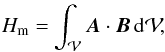 (1)where B is the magnetic field studied over a fixed volume
  . is here a fully closed1 volume bounded by the surface
  . The vector potential, A of B, classically verifies ∇ × A = B as ∇·B = 0 (only approximately true in numerical computations, Valori et al. 2013). The magnetic field B is gauge invariant, meaning that it is unchanged by transformations A → A + ∇ψ, where ψ is any sufficiently regular, scalar function of space and time. Since A is not uniquely defined in general, magnetic helicity requires additional constraints to be well defined. In particular, Hm is a gauge-invariant quantity provided that is a magnetic volume, meaning that the magnetic field is tangent at any point of the surface boundary of :
  , at any time.
Assuming that the volume is fixed, with a flux surface ensuring gauge invariance, the temporal variation of magnetic helicity is derived by direct differentiation of Eq. (1): 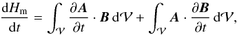 (2)where each of the two integrals on the right-hand side are well defined because they are independently gauge invariant. Given that ∇·(A × ∂A/∂t) = ∂A/∂t·∇ × A − A·∂(∇ × A) /∂t and using the Gauss divergence theorem, we obtain
 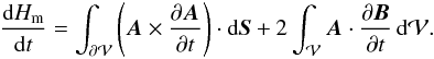 Here, dS is the elementary surface vector, directed outside of the domain . Using Faraday’s law of induction, we derive
 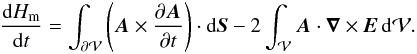 (3)Using again the Gauss divergence theorem, we find that the temporal variation of magnetic helicity is composed of three independently gauge-invariant terms: a volume-dissipative term and two helicity flux terms on the surface of , such that
 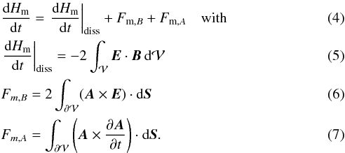 In ideal MHD, where E = −v × B, the volume term is null. For an isolated system, magnetic helicity is thus conserved in the classical sense since its variations are null (cf. Sect. 1). Variations of Hm can only originate from advection of helicity through the boundaries of . The dHm/ dt | diss term corresponds to the dissipation of magnetic helicity of the studied magnetic field in . Taylor (1974) conjectured that this term is relatively small even when non-ideal MHD processes are developing, for example, when magnetic reconnection is present (cf. Sect. 1).
However, because of the gauge-invariance requirement, which imposes that must be a flux surface, magnetic helicity appears as a quantity of limited practical use. In most studied systems, the magnetic field threads the surface and the condition is not fulfilled. In their seminal paper, Berger & Field (1984) have introduced the concept of relative magnetic helicity: a gauge-invariant quantity that preserves essential properties of magnetic helicity while allowing a non-null normal component of the field B through the surface of the studied domain.
2.2. Relative magnetic helicity
In their initial work, Berger & Field (1984) gave a first definition of the relative magnetic helicity as the difference between the helicity of the studied field B and the helicity of a reference field B0 that has the same distribution as B for the normal component along the surface:  .
.
While the definition allows for any field to be used as the reference field, the potential field Bp is frequently used as a reference field in the literature. Since ∇ × Bp = 0, the potential field can be derived from a scalar function φ:  (8)where the scalar potential φ is the solution of the Laplace equation △ φ = 0 derived from ∇·Bp = 0. Given the distribution of the normal component on the surface
  of the studied domain, there is a unique potential field at any instant that satisfies the following condition on the whole boundary of the volume considered:
  (9)Under these assumptions, the potential field has the lowest possible energy for the given distribution of B on (e.g. Eq. (2) of Valori et al. 2012). In the following we also use the potential field as our reference field.
A second gauge-independent definition for relative magnetic helicity has been given by Finn & Antonsen (1985), whose definition we use from here on in this article:  (10)with Ap the potential vector of the potential field Bp = ∇ × Ap. Not only is H gauge invariant, but the gauges of A and Ap are independent of each other, meaning that for any set of sufficiently regular scalar functions (ψ;ψp), H is unchanged by the gauge transformation (A;Ap) → (A + ∇ψ;Ap + ∇ψp). We note that Ap and φ correspond to two distinct solutions of the Helmholtz’s theorem, that is, two distinct non-incompatible decompositions of Bp.
The relative helicity in Eq. (10) can first be decomposed into a contribution that is only due to B, Eq. (1), one that is only due to Bp, and a mixed term: 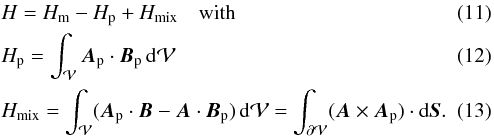 We note that this decomposition is only formal in the sense that each term is gauge dependent and only their sum is actually gauge invariant.
Relative magnetic helicity, as defined in Eq. (10), is equal to the difference between the helicity of the field B and the helicity of its potential field (H = Hm(B) − Hm(Bp)) only if Hmix cancels. Relative helicity is in general not a simple difference of helicity, as for relative energy. A sufficient (but not necessary) condition that ensures the nullity of the mixed term is that A and Ap have the same transverse component on the surface, that is, 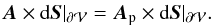 (14)This condition automatically enforces the condition of Eq. (9) on the normal field components. However, it imposes that the choice of the gauge of A is linked with that of Ap. The original definition of Berger & Field (1984) corresponds to a quantity that is less general than the one given by Finn & Antonsen (1985). It is only gauge invariant for particular sets of transformation: (A;Ap) → (A + ∇ψ;Ap + ∇ψp).
Another possible decomposition of relative magnetic helicity from Eq. (10) is (Berger 2003)  where Hj is the classical magnetic helicity of the non-potential, or current-carrying, component of the magnetic field, Bj = B − Bp, and Hpj is the mutual helicity between Bp and Bj. The field Bj is contained within the volume , therefore it is also called the closed-field part of B. Because of Eq. (9), not only H, but also both Hj and Hpj are independently gauge invariant.
2.3. Relative magnetic helicity variation
Assuming a fixed domain , we can differentiate Eq. (10) in time to study the time variations of relative helicity: 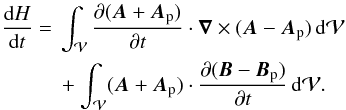 (18)Using the Gauss divergence theorem, we obtain
 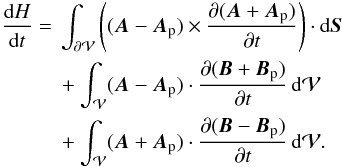 Combining the second and third terms, we find the following synthetic decomposition of the helicity variation in three terms:
 ![\begin{eqnarray} \label{eq:Hvar3} \begin{split} \fdHdt =\ & 2\int_{\vol} \vA \cdot \pardiff{\vB}{t} \dV + \int_{\surf} \left((\vA-\vAp) \times \pardiff{(\vA+\vAp)}{t} \right) \cdot \dS \\ &- 2\int_{\vol} \vAp \cdot \pardiff{\vBp}{t} \dV .\\[-8mm] \end{split} \end{eqnarray}](/articles/aa/full_html/2015/08/aa25811-15/aa25811-15-eq58.png) (19)This decomposition is only formal. Indeed, as for the decomposition of relative helicity of Eq. (11), none of these three terms are independently gauge invariant and only their sum is. The third term can be further decomposed using the scalar potential φ, Eq. (8), and the Gauss divergence theorem:
(19)This decomposition is only formal. Indeed, as for the decomposition of relative helicity of Eq. (11), none of these three terms are independently gauge invariant and only their sum is. The third term can be further decomposed using the scalar potential φ, Eq. (8), and the Gauss divergence theorem: 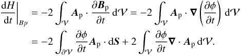 (20)Using the Faraday law and the Gauss divergence theorem, we also obtain
 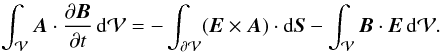 (21)Assuming that at the boundary the evolution of the system is ideal,
 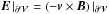 , the surface flux can be written as (e.g., Berger & Field 1984)
 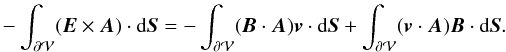 (22)We note that if the evolution of the system is not ideal at the boundary, an additional flux term depending on Enonideal × A, could be added, with Enonideal the non-ideal part of the electric field. This term is here de facto estimated but assumed to be measured as a volume-dissipation term.
Including Eqs. (20)−(22) in Eq. (19), the variation of magnetic helicity can thus be decomposed as 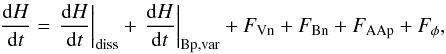 (23)with
 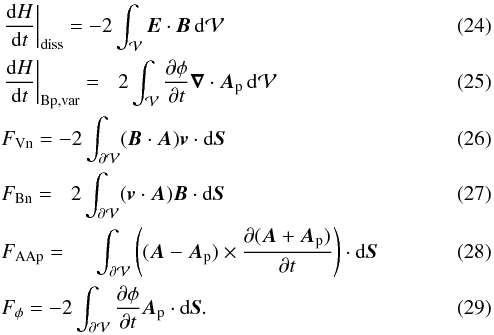 The dH/ dt | diss term is a volume term that corresponds to the actual dissipation of magnetic helicity of the studied magnetic field (Eq. (5)). The dH/ dt | Bp,var term, which, despite being a volume term, is not a dissipation, traces a change in the helicity of the potential field. As B evolves, its distribution at the boundary implies a changing Bp (Eq. (9)). The helicity of the potential field, not necessarily null, therefore evolves in time. More precisely, the potential field is only defined in terms of its boundary values. However, this is not true in general for the vector potential of the potential field because of the gauge freedom. Hence, the helicity of the potential field cannot in general be expressed as a function of boundary values alone, except for the particular case of a vector potential without sources or sinks in , which is the case when the Coulomb gauge is used. Therefore, the time variation of the helicity of the potential field necessarily contains both volume and flux contributions.
All the other terms are flux terms that correspond to the transfer of helicity through the surface boundary . The FVn and FBn are sometimes called the “emergence” and “shear” terms, but such a characterization can be misleading because their contributions depend on the gauge selected for A. The FAAp term is related to a cross contribution of A and Ap. Finally, Fφ corresponds to a flux of the helicity of the potential field.
The dH/ dt | diss term is the only term of the decomposition that is gauge invariant. All the other terms are not independently gauge invariant. This means that the relative intensity of these terms is different for different gauges. Combined, they produce the same gauge-invariant value of dH/ dt. We study the dependence of this decomposition on the chosen gauge in Sect. 5. We also note that the total flux Ftot of relative helicity,  (30)is only gauge invariant for A but not for Ap.
Moreover, unlike dH/ dt | diss, dH/ dt | Bp,var is not a priori null in ideal MHD. This implies that dH/ dt cannot be written in a classical conservative form since dH/ dt | Bp,var cannot be strictly written as a flux term. Therefore relative magnetic helicity is not a priori a conserved quantity of MHD in the classical sense: its variation in may not solely come from a flux of relative helicity through the boundary. Relative magnetic helicity may not be conserved even if dH/ dt | diss is small. The conservation of relative helicity and the dissipation of magnetic helicity are thus two distinct problems: the relative intensity of these terms will vary, depending on which gauge is employed, as we illustrate in Sect. 5.
2.4. Relative magnetic helicity variation with specific gauge conditions
While the variation of magnetic helicity can be generally described by Eq. (23) for any gauge, the choice of some specific additional constraint on the gauge allows simplifying the expression of dH/ dt and possibly its computation.
2.4.1.  condition
We note that with the specific condition 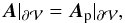 (31)the condition of Eq. (14) is necessarily satisfied thus FAAp = 0 and the terms FVn and FBn can be expressed only in terms of Ap. Thus, the helicity variation, Eq. (23), simplifies as
 ![\begin{eqnarray} \begin{split} \label{eq:HvarcondAAp} \left. \fdHdt\right |_{\rm Cond.~ (\text{\ref{eq:CondA=Ap}})} = &-2\int_{\vol} \vE \cdot \vB \dV +2\int_{\vol}\pardiff{\phi}{t} \divAp \dV \\ &-2\int_{\surf} (\vB \cdot \vAp) \vv \cdot \dS +2\int_{\surf} (\vv \cdot \vAp) \vB \cdot \dS \\ &-2\int_{\surf} \pardiff{\phi}{t} \vAp \cdot \dS.\\[-8mm] \end{split} \end{eqnarray}](/articles/aa/full_html/2015/08/aa25811-15/aa25811-15-eq80.png) (32)We note that in this derivation the vector potential A is absent. Condition (31) removes the need of computing A to estimate the helicity variations. However, to derive H from Eq. (10), both A and Ap must be computed with gauges coupled with Eq. (31). Then, one must strictly control that this condition is enforced throughout the surface of the studied system. This can be numerically challenging.
(32)We note that in this derivation the vector potential A is absent. Condition (31) removes the need of computing A to estimate the helicity variations. However, to derive H from Eq. (10), both A and Ap must be computed with gauges coupled with Eq. (31). Then, one must strictly control that this condition is enforced throughout the surface of the studied system. This can be numerically challenging.
To determine the helicity dissipation, we here compare time-integrated helicity flux with direct helicity measurements. As our numerical method does not allow us to enforce Eq. (31), we cannot use the simplified Eq. (32) to compute the helicity variation.
2.4.2. Coulomb gauge for the potential field: ∇·Ap = 0
If to determine the potential field one decides to choose the Coulomb gauge,  (33)then there is no volume variation of the helicity of the potential field dH/ dt | Bp,var = 0. The helicity variation can be reduced to the simplified form
 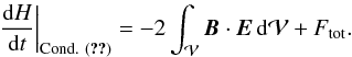 (34)Using the coulomb gauge for the potential field, we observe that the variation of the relative magnetic helicity is given by a flux of helicity through the boundary and the dissipation term dH/ dt | diss. Relative magnetic helicity to a reference field expressed in the Coulomb gauge can therefore be written with a classical conservative equation.
2.4.3. Boundary null Coulomb gauge
Condition (33) does not enforce a unique solution for Ap. It is possible to further constrain the Coulomb gauge if the vector potential Ap satisfies the additional boundary condition  (35)With this additional constraint, the flux of helicity of the potential field is null, Fφ = 0. Then, with conditions (33) and (35), the helicity variation thus reduces to the form
 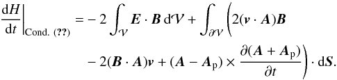 (36)
(36)
2.4.4. Simplified helicity flux
Including the three conditions of previous subsections, that is, 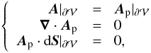 (37)we obtain the well-known expression for the simplified helicity flux (e.g., Berger & Field 1984; Pariat et al. 2005):
 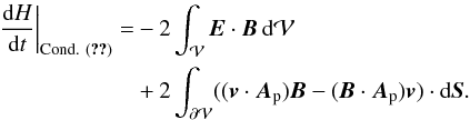 (38)With this set of conditions, the flux terms FVn and FBn are fully fixed. However, we recall that these terms remain gauge dependent: using a gauge where the conditions of Eq. (37) are not fully enforced would lead to a different Ap and A, consequently, to a different distribution of helicity flux between FVn, FBn and other terms. It is therefore theoretically incorrect to study them independently.
Equation (38) is the classical formulation for the helicity flux that has been derived by Berger & Field (1984) for an infinite plane. However, for a 3D cubic domain this formulation is only valid if all the conditions of Eq. (37) are satisfied. While Yang et al. (2013) have used Eq. (38) to compute the helicity flux, it remains to be determined whether all conditions (37) are fulfilled when computing the volume helicity. Their relatively high level of non-conservation (3%) in the ideal phase of the evolution of their system may be related to this discrepancy. Finally, while the conditions of Eq. (37) can drastically simplify the estimation of the helicity variation, they strongly constrain the numerical implementation of A and Ap. Fast, precise, and practical numerical computation of the vector potentials may require a different choice of gauge.
3. Methodology
This section describes the methodology employed in our numerical experiments. In Sect. 3.1 we present the general method used to estimate the relative magnetic helicity conservation and the magnetic helicity dissipation. Then in Sect. 3.2 we describe how we practically computed the volume helicity and its flux. Finally, in Sect. 3.3 we present the numerical data set considered for the helicity conservation tests.
3.1. Estimators of magnetic helicity conservation
Following Yang et al. (2013), we computed the volume variation along with the flux of magnetic helicity. From two successive outputs of the studied MHD system, corresponding to two instant τ and τ′, separated by a time interval Δt, we directly computed their respective total helicity  and
and  in the volume using the method of Sect. 3.2, and then, the helicity variation rate between these 2 instants:
  . We simultaneously estimated the different sources of fluxes F# through the surface of the domain, with # the different contribution to the total flux in Eq. (30).
We also integrated the helicity fluxes at the boundary  in time,
 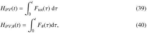 with # the different contribution to the total flux of Eq. (30).
We note that two very different methods were used to compute  and . To derive (and
  ) from Eq. (10), only three components of the magnetic field B in the whole domain are needed: A,Bp,andAp, are derived from B (cf. Sect. 3.2). For (and Ftot), only data along the boundary are required. Furthermore, the helicity flux estimation requires the knowledge of the three components of the velocity field on (to compute FVn and FBn). These quantities are not used to compute . The methods of estimating and are thus fully independent.
A physical quantity is classically said to be conserved when its time variation in a given domain is equal to its flux through the boundary of the domain (cf. Sect. 1). To study the twofold problem of the conservation of relative magnetic helicity and the dissipation of magnetic helicity, we used two quantities, Cr and Cm respectively.
 |
Fig. 1 Snapshots of the magnetic field evolution during the generation of the jet. The red field lines are initially closed. The green and white field lines are initially open. All the field lines are plotted from fixed footpoints. The red and white field lines are regularly plotted along a circle of constant radius, while the green field lines are plotted along the x-axis. At t = 900 the system is in its pre-eruption stage. It is close to the maximum of energy and helicity. All the helicity is stored in the close domain. At t = 1000 the system is erupting. Numerous field lines have changed their connectivity, as can be observed from the open red field lines and the closed white field lines. Helicity is ejected upward along newly opened reconnected field lines. At t = 1500 the system is slowly relaxing to its final stage. |
For relative magnetic helicity to be perfectly conserved, we must have  , or dH/ dt equal to Ftot, or in other words, the volume terms of the relative helicity variation should be null. By estimating Cr,
 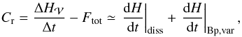 (41)it is possible to determine the level of conservation of relative magnetic helicity. As already noted in Sect. 2.3, even if B evolves within the ideal MHD paradigm, the relative magnetic helicity evolution cannot be written with a classical equation of conservation because the term in dH/ dt | Bp,var is not a flux integral through a boundary and generally does not vanish.
Second, we determined the dissipation of the magnetic helicity of the studied field (Eq. (24)), by estimating Cm equal to 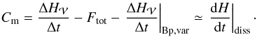 (42)Our estimation of Cm was made independently of the estimation of dH/ dt | diss. Our method thus does not require the knowledge of the electric field E, which is a secondary quantity in most MHD problems. The dissipation is thus estimated in a way that is completely independent of the non-ideal process, for instance, of the precise way magnetic reconnection develops.
As the estimators measure both physical helicity variations and numerical errors, we used different non-dimensional criteria to quantify the level of helicity conservation and the precision of our measurements. We computed the relative accumulated helicity difference ϵH,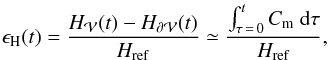 (43)with Href a normalizing reference helicity, which is physically significant for the studied system (e.g., the highest value in the studied interval).
At each instant, Cm expresses the rate of dissipation of helicity, that is, our numerical estimation of Eq. (24). It can include artifact fluctuations that are due to the numerical precision of the flux estimation and the time derivation of . In addition, because helicity is a signed quantity, both positive and negative helicity can be generated by non-ideal effects. It may be relevant to know the time-integrated absolute variation of helicity as a function of time. Hence, we defined another metric, ϵCm, 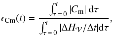 (44)where the absolute values guarantee that we take an upper limit of the dissipation. Along with ϵH, ϵCm allows us to evaluate the level of dissipation and the numerical precision of our measurements. The measure of a low value of ϵCm and ϵH can thus provide a clear demonstration of the level of conservation of relative magnetic helicity. For two methods with similar ϵH, a higher value of ϵCm would indicate measurements presenting larger numerical errors.
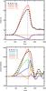 |
Fig. 2 Top panel: time evolution of the different magnetic energies relative to their respective initial values: total ( |


3.2. Volume helicity and flux computations in the DeVore gauge
To compute magnetic helicity in the volume, , we used the method presented in Valori et al. (2012). All the vector potentials were computed using the gauge presented in DeVore (2000), without a vertical component: 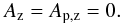 (45)Under this assumption, the vector potentials were computed in the volume using a 1D integral (cf. Eqs. (10) or (11) of Valori et al. 2012) with a 2D partial differential equation to be solved at the bottom or top boundary (cf. Eqs. (9) or (12) of Valori et al. 2012). We tested that we did not obtain significant differences on the helicity conservation and dissipation properties, whether the integration was made from the top or the bottom boundary of the system. Our results here were obtained with the integration performed from the top boundary.
While other gauge choices could be explored, choosing the DeVore gauge, Eq. (45), is here motivated by the fact that it is numerically efficient and convenient. This selection leaves a freedom for the gauge of A and Ap, which can be independent, that is, not linked as in Eq. (31). In our computation of Ap and A, we used gauge freedom to additionally enforce that the two vectors are equal at the top (see Eq. (29) of Valori et al. 2012),  (46)We still have a freedom on Ap(ztop), as expressed by the 2D partial differential equation (20) of Valori et al. (2012). Here, we selected their particular solution expressed by their Eqs. (24), (25). With this additional choice, both Ap and A are uniquely defined (modulo a constant) by vertical integration starting from the top boundary.
Practically, we first determined the potential field by solving the solution of the Laplace Eq. (17) for φ of Valori et al. (2012). Then we computed the potential vectors from a direct 1D integration of Bz starting from the top boundary (cf. Sect. 3.3 of Valori et al. 2012). We refer to this method below as the “practical DeVore method” since it is efficient and easy to implement.
While condition (46) holds at the top boundary, it does not hold at the other boundaries. Indeed, Eq. (13) in Valori et al. (2012) can be used to show that the difference between the value of Ap and A at the bottom boundary is equal to  . It is important to note that the conditions of Hmix = 0 and
  are never enforced in this gauge. The relative helicity terms Hmix and Hp and the helicity flux term FAAp and Fφ can thus never be considered null (see also Valori et al. 2012,for more details). For the practical DeVore method, the helicity variation of the system is therefore given by the general formula of Eq. (23).
Alternatively, we determined the helicity assuming a Coulomb gauge for Ap alone. The DeVore and Coulomb gauge are indeed compatible for a potential field. We solved the 2D partial differential Eq. (20) of Valori et al. (2012) as a Poisson problem to obtain Ap (see their Eq. (41), but translated to the top boundary). This implies by construction that Ap is simultaneously respecting the DeVore, Eq. (45), and the Coulomb gauge, Eq. (33). In the following, we refer to this method as the DeVore-Coulomb method.
While still following the DeVore condition (45), A computed in the DeVore-Coulomb method will be different from A computed in the practical DeVore method because the boundary condition, Eq. (46), is different. In particular, the distributions of A at the bottom boundary will be significantly different with each method and hence will lead to very different values of FBn and FVn. In Appendix A, we present an additional test, with Ap computed in the Coulomb gauge, but where A does not satisfy condition (46).
3.3. Test data set
To test the helicity conservation, we employed a test-case 3D MHD numerical simulation of the generation of a solar coronal jet Pariat et al. (2009). Figure 1 presents snapshots of the evolution of the magnetic field. The simulation assumes an initial uniform coronal plasma with an axisymmetric null-point magnetic configuration (left panel). The magnetic null point was created by embedding a vertical dipole below the simulation domain and adding a uniform-volume vertical magnetic field of opposite direction in the domain. The null point presents a fan-spine topology that divides the volume into two connectivity domains, one closed and surrounding the central magnetic polarity, and one open.
The computation was performed with non-dimensional units. We analyzed the time evolution of the magnetic field from t = 0 to t = 1600. The time steps between two outputs were Δt = 50 for t ∈ [ 0;700 ] during the accumulation phase and Δt = 10 for t ∈ [ 700;1600 ] during the dynamic phase of the jet. The analysis volume is a subdomain of the larger discretized volume employed in the original MHD simulation: [−6,6 ] in x-, [−6,6 ] in y-, and [ 0,12 ] in the z-directions, thus only taking into account the region of higher resolution (cf. Fig. 1 of Pariat et al. 2009).
The ideal MHD equations were solved with the ARMS code based on flux-corrected transport algorithms (FCT, DeVore 1991). The parallelization of the code was ensured with the PARAMESH toolkit (MacNeice et al. 2000). In the original simulation of Pariat et al. (2009), reconnection is strongly localized thanks to the use of adaptive mesh-refinement methods at the location of the formation of the thin current sheets involved in reconnection (cf. Appendix of Karpen et al. 2012). To keep the resolution of the domain constant, we here switched off adaptivity, however, so that the resolution is equal to the initial one (as in Fig. 1 of Pariat et al. 2009), throughout the whole simulation.
The variation of energies relative to their initial value,  is displayed in the top panel of Fig. 2. The index indicates that the energy is computed by volume integration. The total energy,
  , in the domain can be decomposed as
  (47)where
  and
and  are the energies associated with the potential and current-carrying solenoidal contributions, and
  is the sum of the nonsolenoidal contributions (see Eqs. (7) and (8) in Valori et al. 2013,for the corresponding expressions). Initially, the system is fully potential and
  . Energy is injected in the system by line-tied twisting motions of the central polarity. The axisymmetric boundary motions preserve the distribution of Bz at the bottom boundary. Magnetic free energy and helicity accumulates, which monotonically increases the twist in the closed domain (Fig. 1, central left panel). The potential field energy
  decreases slightly during the accumulation phase because of the bulge of the central domain, which changes the distribution of the field on the side and top boundaries. The
  term is almost constantly null, an indication of the excellent solenoidality of the system
Around t ≃ 920, the system eventually becomes violently unstable: magnetic reconnection sets in, and the closed twisted field lines reconnect with the outer open field lines. A steep decrease in the free magnetic energy is observed in Fig. 2: 83% of the maximum free magnetic energy is dissipated, ejected, or transformed. Through reconnection, twist and helicity are expelled from the central domain, inducing a large-scale kink wave that exits through the top boundary (Fig. 1, central right panel). This large-scale nonlinear magnetic wave simultaneously compresses and heats the plasma, inducing the generation of an untwisting jet that can observationally be interpreted as a blowout jet (Patsourakos et al. 2008; Pariat et al. 2015). The driving motions had been slowly ramped down at the time of the trigger of the jet, so that little energy and helicity are injected from the lower boundary after the jet onset (cf. Fig. 6 of Pariat et al. 2009). The system slowly relaxes in the final stage to a configuration similar to its initial state, with the potential field energy being similar to its initial value and only few field lines remaining twisted, next to the inversion line (Fig. 1, right panel).
This simulation thus presents two distinct phases that are typical of active events: before t ≃ 920, a phase with a slow ideal accumulation of magnetic helicity and energy, and after t ≃ 920, an eruptive phase of fast energy dissipation and helicity transfer involving non-ideal effects. In the first phase, the system behaves very similarly to ideality, as demonstrated in a benchmark with a strictly ideal simulation (Rachmeler et al. 2010). In the non-ideal phase, Pariat et al. (2009) showed that 90% of the helicity was eventually ejected through the top boundary by the jet, and Pariat et al. (2010) showed the high reconnection rate processing the magnetic flux during the jet. These two phases allow us to test the conservation of helicity in two very distinct paradigms of MHD.
In the following we test the helicity conservation with the above MHD simulation. We first use the practical DeVore method (see Sect. 4). We next test the effect of the gauge choice on our results by using the DeVore-Coulomb method (see Sect. 5). We show how the gauge choice can affect the evolution of each term.
4. Magnetic helicity conservation in the practical DeVore gauge
Our first study of the helicity variations was performed in the practical DeVore gauge. The only assumptions on the potential field and the vector potentials are given by Eqs. (9), (45), and (46). This corresponds to a general case where the helicity variation of the system is provided by Eq. (23).
4.1. Helicity evolution
The bottom panel of Fig. 2 presents the evolution of the relative magnetic helicity in the system. Similarly to magnetic energy, the two phases of the evolution are clearly marked. The first phase corresponds to a steady accumulation of magnetic helicity, while the second corresponds to the blowout jet. The latter is associated with a steep decrease of magnetic helicity. As the system relaxes, the magnetic helicity value oscillates. These oscillations are related to the presence of a large-scale Alfvénic wave, which is slowly damped after the jet. This oscillations can also be seen in the total energy but with a much smaller relative amplitude (so small that still decreases monotonically).
The right panel of Fig. 2 also presents the decomposition of the relative magnetic helicity, , in Hm, Hmix and Hp of Eqs. (11)−(13). During the accumulation phase, is dominated by Hmix, while Hp is almost constantly null. During the jet, strong fluctuations of the relative importance of these terms are visible. Hm, Hmix and Hp eventually present contributions of similar amplitude. However, because these terms are not gauge invariant, their value in a different gauge might be quite different (cf. Sect. 5).
The decomposition of with Hj and Hpj of Eqs. (15)−(17) is also plotted in Fig. 2, bottom panel. Hj has an evolution comparable to  . It captures most of the helicity evolution during both the accumulation and jet phases. In contrast, the mutual helicity between the potential and the current-carrying fields contains mostly oscillations. Therefore, Hj, which is a gauge invariant quantity, is a promising quantity to analyze during a jet or eruption.
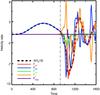 |
Fig. 3 Comparison of the helicity variation rate and the helicity flux computed in the practical DeVore gauge. The helicity variation rate ( |
4.2. Helicity fluxes
We computed the time variations of the helicity determined with the volume-integration method and compared it with the different terms of the relative magnetic helicity flux through the whole system boundary (Fig. 3). This shows that the helicity variation very closely matches the curve of Ftot, indicating that the variation of helicity in the domain is tightly related to the flux of relative helicity through the boundary. The core result of this study is that indeed magnetic helicity is very well conserved in the studied simulation during both the quasi-ideal-MHD and non-ideal phases.
During the non-ideal/jet phase, strong fluctuations are observed for all terms except for the FAAp term. The latter is constantly negligible compared to the others. On the other hand, the Fφ term displays strong fluctuations, frequently of similar amplitude and opposite sign to FBn. The Fφ term clearly cannot be neglected in this gauge.
The analysis of the flux of each term through each individual boundary is enlightening (Fig. 4), although we recall that the plotted terms are not gauge invariants. Although its amplitude is extremely small, a finite flux of FAAp is present only at the bottom boundary during the whole evolution of the system: there is no flux on the sides because of the DeVore gauge (Eq. 45) and no flux on the top because of the imposed condition of Eq. (46).
During the ideal phase, the flux of helicity is completely dominated by the FBn term that originates from the bottom photospheric boundary. This is consistent with the fact that the system is indeed driven by horizontal shearing motions at the bottom boundary. No remarkable helicity flux is observed at the other boundaries during this period. Helicity is thus accumulating in the volume .
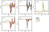 |
Fig. 4 Total helicity flux, Ftot (Eq. (30)), and the terms compositing it, Eqs. (26)−(29), through the different boundaries computed in the practical DeVore gauge. a) Ftot; b) Fφ; c) FAAp; d) FBn; and e) FVn. In each plot the dark line corresponds to the sum of the flux through all the boundaries, while the color lines correspond to a flux through a particular boundary (purple and blue: left and right x sides, green and orange: front and back y sides; yellow and red: bottom and top z sides). |
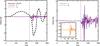 |
Fig. 5 Difference between the helicity variation rate and the boundary helicity flux computed in the practical DeVore gauge. The relative helicity conservation criterion Cr (red line, Eq. (41)) and the magnetic helicity dissipation criterion Cm (blue line, Eq. (42)) are plotted relative to the helicity variation rate ( |
During and after the jet (t> 920), strong helicity fluxes are noted in the side and top boundaries, while the bottom flux is now negligible because the boundary flows have been decreased in amplitude. A strong helicity flux occurs at the top boundary (red curves), dominated by the FBn term and to a lesser extend by the FVn term. This corresponds to the ejection of helicity by the jet, driven by a large-scale nonlinear torsional wave (Pariat et al. 2009, 2015). FVn peaks at the time of the passage of the bulk of the jet through the top boundary. The flux of FBn and FVn through the side boundaries, while present, is comparatively low. However, the side boundaries see the transit of important flux Fφ. No specific side boundary dominates the total value of Fφ. As a result of the DeVore gauge (Eq. (45)), Fφ is null at the bottom and top boundaries.
We conclude that when it is computed with the particular DeVore method, the total flux of helicity Ftot during the jet consists of a complex transfer of helicity through all the boundaries of the system.
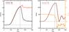 |
Fig. 6 Left panel: comparison of the evolution of magnetic energy ( |


4.3. Helicity conservation
To better estimate the helicity conservation and dissipation, we plot in Fig. 5 the criteria Cr and Cm (see their definition in Sect. 3.1). We observe that these two criteria are almost equal. They differ only by the term describing the volume variation of the potential helicity dH/ dt | Bp,var of Eq. (26). Our calculation finds that dH/ dt | Bp,var is extremely small compared to the variation of Cr and Cm (see inset in the right panel of Fig. 5), even though we did not explicitly enforce ∇·Ap = 0. This term is smaller than the combined effect of the real helicity dissipation dH/ dt | diss and the numerical errors on the volume and flux helicity measurements.
The curve of Cr demonstrates that magnetic helicity is extremely well conserved during the ideal-MHD phase of the simulation and that it is also very well conserved during the non-ideal phase. Moreover, the amplitude of | Cm | does not exceed 0.029 during the ideal phase, which is 1% of the maximum amplitude of helicity variation during the period. At the end of this period, we also have ϵCm(t = 920) < 1%, thus helicity is very weakly dissipated, as theoretically expected (Woltjer 1958).
During the non-ideal phase, Cr and Cm show high frequency fluctuations around the null value, decorrelated from the fluctuation of helicity in the system. Our analysis indicates that while these fluctuations might originate from the real physical term dH/ dt | diss, they are in fact dominated by the numerical precision on the estimation of Ftot. From the same simulations data, we show in Sect. 5 that the computation with the DeVore-Coulomb method reduces these fluctuations.
In Fig. 6 we plot the variation of magnetic energy and helicity in the system computed with a volume integration and from the integration of the Poynting and helicity fluxes through the boundaries of the system. During the ideal-MHD phase, both magnetic energy and helicity are well conserved, their volume variations being equal to their boundary fluxes. While magnetic helicity is still very well conserved during the non-ideal phase, magnetic energy is clearly not. When the jet is generated, the magnetic energy quickly decreases: part of it is ejected through the top boundary by the jet, but for most part it dissipates in the reconnection current sheet and is transformed into other forms of energy. When the simulation is stopped, we determined that about 17% of the magnetic energy injected in the system by the bottom boundary motions remains in the system, 21% is directly ejected with the jet, and the remaining 62% are dissipated or transformed into other forms of energy (see also Pariat et al. 2009). As expected during reconnection, magnetic energy is strongly non-conserved.
The situation for magnetic helicity is very different. At the end of the ideal phase, the maximum difference between and is of 3.5 units. During this period, a total of Href = max(H) = 1265 units are injected and only a fraction ϵH(t = 920) = 0.3% is lost. The ideality of the system is thus very well maintained. During the non-ideal phase, the maximum difference between and is equal to 58 units (orange line, Fig. 6, right panel) and ϵH(t = 1600) = 4.5%. The jet is able to transport away a huge portion, 77% of the helicity of the system. Finally, about 19% of the helicity remains in the system at t = 1600, while still slightly oscillates (Fig. 6, right panel).
To summarize, we have thus confirmed with a generic gauge for solar-like events the hypothesis of Taylor (1974) that magnetic helicity is very well conserved even when non-ideal processes are acting. The relative helicity dissipation is 15 times smaller that the relative magnetic energy dissipation. However, with the practical DeVore Gauge, we observed that Cm fluctuates strongly, possibly limited by numerical precision. We now wish to test whether we can obtain better results with a different gauge, simultaneously allowing us to test the gauge invariance of the different helicity variation terms.
5. Magnetic helicity conservation in the DeVore-Coulomb case
Relative magnetic helicity has been defined as a gauge-invariant quantity (see Sect. 2.3). However, the surface flux of relative helicity is not, neither are the individual terms that define the flux. In the following we study the influence of computing magnetic helicity using a different gauge. The vector potential of the potential field, Ap, is now computed in the DeVore-Coulomb gauge, but not A (since the Coulomb gauge is only compatible with DeVore gauge for a potential field). Because we also impose the condition of Eq. (46), A is also recomputed with our DeVore-Coulomb method, however (see Sect. 3.2). We briefly discuss in Sect. A the case where Eq. (46) is not enforced.
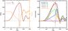 |
Fig. 7 Left panel: evolution of the magnetic helicity computed with the practical DeVore method (dashed line) and with the DeVore-Coulomb method (red line). Their difference is plotted with an orange line (cf. right axis). Right panel: volume magnetic helicity ( |
5.1. Gauge dependance
In Fig. 7 we plot the evolution of the relative magnetic helicity, in the DeVore-Coulomb gauge for Ap. The left panel shows the comparison with the same quantity computed using the practical DeVore gauge, used in the previous section. We observe that the two curves match almost perfectly. Their maximum differences is at most 3.5 units, and their maximum relative helicity difference is 0.3%. The gauge invariance is thus very well respected for our estimation of the relative magnetic helicity.
In the right panel of Fig. 7 we plot the decomposition of the relative magnetic helicity. Unlike with the gauges of the practical DeVore method (cf. Fig. 2), Hp is now almost constantly null. It is not strictly null since we did not impose  on the side boundaries. We see that when the jet developes, Hp fluctuates slightly (barely visible in Fig. 7). The helicity is thus distributed differently between Hm, Hmix and Hp in the DeVore-Coulomb case than in the practical DeVore gauge. As expected, these helicity terms are indeed not gauge invariant. Most of the helicity that was carried by Hp for the practical DeVore gauge is now carried by Hm, while Hmix remains very similar in both gauges (compare the green curves in Figs. 2 and 7). In general, we have to expect a completely different distribution of Hm, Hmix, and Hp in other gauges. On the other hand, the quantity Hj and Hpj remains equal in both gauge computation (with the same precision as ). This is expected since Hj and Hpj are gauge-invariant quantities.
For the helicity fluxes, the time variations of the helicity in the DeVore-Coulomb case tightly follows the helicity flux through the boundary (Fig. 8, left panel). While is gauge invariant, the different contribution of Ftot are not. By comparison with Fig. 3 one observes that FBn, FVn, and Fφ have a very different evolution. While Fφ was presenting fluctuations of the same amplitude as Ftot in the practical DeVore gauge, this term is now very weak throughout the evolution of the system with the DeVore-Coulomb method. The FBn term dominates Ftot in the DeVore-Coulomb case during both the ideal MHD phase (at the bottom boundary) and during the non-ideal period (at the top boundary). FVn is weaker than with the practical DeVore gauge. The FAAp term remains negligible in both cases, although with a different choice of gauge, FAAp can contribute significantly to Ftot (see Appendix A).
The effect of the gauge dependance is more strikingly illustrated for the time-integrated helicity fluxes  (Eq. (40)) through the boundaries. Their evolution is presented in Fig. 9 for the two gauge computations. While remains gauge invariant (Fig. 7, left panel), the present different profiles in the different gauges, as expected.
  is small when computed with the DeVore-Coulomb gauge, while it presents large amplitudes in the practical DeVore gauge.
  and
and  present lower mean absolute values when Ap follows the DeVore-Coulomb conditions. Their ratio also strongly depends on the set of gauges employed.
Numerous studies have computed  and
and  and followed their time evolution in observed active regions (e.g., Zhang et al. 2012; Liu et al. 2013, 2014b,a). These terms have been incorrectly called “emergence” and “shear” terms, and it was attempted to extract physical insight from their values and respective ratio. However, as these terms are not gauge invariant, one must question the pertinence of such results. and cannot be studied independently because for a given v, their intensities and respective values can be simply modified by a change of gauge. This extends the conclusion of Démoulin & Berger (2003), who showed that only the sum of and can be derived when only the tangential velocity components are known. More generally, the study presented here shows that even when the full velocity field on the boundary is known, and can present different values depending on the gauge used for the computation. In summary, only the sum
  of all the flux terms, , carries meaningful information.
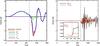 |
Fig. 8 Left panel: comparison of the helicity variation rate and the helicity flux integrated through the six boundaries of the domain in the DeVore-Coulomb case. The plotted curves are similar as in Fig. 3. Right panel: magnetic helicity dissipation criterion Cm, Eq. (42), plotted for the practical DeVore (black line) and the DeVore-Coulomb (red line) methods. The inset shows ϵCm, Eq. (44), with the same color convention. |
5.2. Helicity dissipation
The estimators Cr and Cm (cf. Sect. 3.1) enable us to study the helicity conservation and dissipation. Since dH/ dt | Bp,var is null because of the Coulomb condition in the potential field, Cm and Cr are equal to our numerical precision. There is no volume helicity variation due to the potential field. The conservation of the relative helicity is only limited by the actual dissipation helicity dH/ dt | diss. The curve of Cr for the DeVore-Coulomb computation confirms that magnetic helicity is gauge-invariantly well conserved during the simulation (Fig. 8, right panel).
Our estimation of the helicity dissipation is even improved in the DeVore-Coulomb case. During the quasi-ideal phase Cm is equal to its value with the practical DeVore case. However, we observe that in the non-ideal phase, Cm presents smaller oscillations when computed in the DeVore-Coulomb case. Because Cm is equal to the helicity dissipation, dH/ dt | diss, it should theoretically be gauge invariant, but Cm can change by a factor 2 when computed with the different methods. With the practical DeVore method, the fluctuations of Cm peak at 25% of the maximum amplitude of helicity variation during the non-ideal phase, while the peak is only equal to 4.5% of the amplitude in the DeVore-Coulomb case. The non-dimensional criterion ϵCm at the end of the simulation is equal to 7% in the practical DeVore case, while it is limited to 2.7% with the DeVore-Coulomb method (see the inset in Fig. 8, right panel).
While we measured with a high precision (see above), the estimation of the helicity flux, Ftot induces more numerical errors. The high-frequency oscillations observed in the different terms contributing to Ftot are caused by the lower level of precision. The criterion Cm is equal to the helicity dissipation plus the numerical errors in the volume helicity variations and in the helicity flux. Actually, Cm provides is an upper value for the helicity dissipation. In the DeVore-Coulomb case, Cm probably provides a lower value, hence a better constraint on dH/ dt | diss, because the Ftot is dominated by the errors on FBn, while in the practical DeVore case, the errors of the fluctuating FBn, FVn and Fφ have comparable magnitudes.
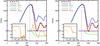 |
Fig. 9
|


The measure of the helicity flux through the boundary is the limiting factor that does not permit us to reach numerical precision during the non-ideal phase. A higher spatial resolution sampling of the velocity field on the boundary sides will probably further improve the helicity dissipation estimation. Our present computation of Cm is therefore only an upper bound on the real helicity dissipation dH/ dt | diss. Because of its lower ϵCm, the DeVore-Coulomb method allows us to better bound the helicity dissipation.
In a DeVore-Coulomb computation, the maximum difference between and is of now of 4.3 units and ϵH(t = 920) = 0.3% during the ideal-MHD phase. As theoretically expected, the dissipation of magnetic helicity is extremely small when only ideal processes are present. This demonstrates that the ideality of the system is very well maintained by the numerical scheme during that phase. At the end of the non-ideal phase, the maximum difference between and is equal to 28.2 units (orange line, Fig. 9, right panel), and the relative amount of helicity dissipated is smaller than ϵH(t = 1600) = 2.2%.
In absolute values, the dissipation of magnetic helicity is thus much smaller than the magnetic helicity, which is ejected. The dissipated helicity represents less than 3% of the helicity carried away by the jet. To track the helicity evolution of this jet system, the helicity dissipation only represents a very minor contribution, more than one order of magnitude smaller than the helicity that remains in the system and the ejected helicity.
This low helicity dissipation is also to be compared to the relative decrease of magnetic energy of 62%, which develops simultaneously. The reconnections generating the jets are thus dissipating or transforming magnetic energy ≳30 times more efficiently than magnetic helicity is dissipated. While vast amounts of energy are lost, magnetic helicity is barely affected by the non-ideal MHD processes at play.
6. Conclusion
Based on the property that magnetic helicity presents an inverse cascade from small to large scale, Taylor (1974) conjectured that magnetic helicity, similarly to pure ideal MHD, is also effectively conserved when non-ideal processes are present. Because of the inherent difficulties in measuring magnetic helicity, tests of this conjecture have so far been very limited (cf. Sect. 1). The theoretical development of relative magnetic helicity (Berger & Field 1984) and the publication of recent methods for measuring relative magnetic helicity in general 3D datasets (Thalmann et al. 2011; Valori et al. 2012; Yang et al. 2013) are now opening direct ways to test the conservation of magnetic helicity.
We here performed the first precise and thorough test of the hypothesis proposed by Taylor (1974) in a numerical simulation of an active solar-like event: the impulsive generation of a blowout jet (Pariat et al. 2009). Following Yang et al. (2013), our methods for testing the level of magnetic helicity dissipation relies on the comparison of the variation of relative helicity in the domain with the fluxes of helicity through the boundaries.
This led us to revise the formulation of the time variation of relative magnetic helicity in a fully bounded volume (cf. Sect. 2.3). As relative magnetic helicity relies on magnetic vector potential, the question of the gauge is a central problem of any quantitiy related to magnetic helicity. A general decomposition of the gauge-invariant time variation of magnetic helicity is given in Eq. (23), with no assumption made on the gauges of the magnetic field and of the reference potential field. Furthermore, we discussed how specific gauges and combination of gauges can simplify the formulation of the helicity variation (Sect. 2.4).
Following (Valori et al. 2012), we computed the variation of relative magnetic helicity using different gauges, all of them based on the gauge of Eq. (45) suggested by DeVore (2000). We were able to test the gauge dependance of several terms entering in the decomposition of relative magnetic helicity and its time variation. We demonstrated that all the quantities that were theoretically gauge invariant (H, Hj, Hpj, dH/ dt) were indeed invariant with a very good numerical precision (<0.3% of relative error).
Additionally, our analysis showed the effect of using different gauges on gauge-dependant quantities. Of particular interest are the results that we obtained for the FVn and FBn terms, Eqs. (26), (27), entering in the decomposition of the helicity flux. In some studies (e.g., Liu et al. 2014b,a), these terms have been used to putatively track the helicity contribution of vertical and horizontal plasma flows. However, our computations illustrate that these fluxes (and their ratio) vary with the gauges used, hence preclude any meaningful physical insight into their interpretation in terms of helicity. Following Démoulin & Berger (2003), we concluded that only the total helicity flux, Ftot, conveys a physical meaning.
Unlike magnetic helicity, we showed that relative magnetic helicity cannot be expressed in general in classical conserved form, even in ideal MHD. Only when computing the reference potential field with the Coulomb gauge can the variation of the relative magnetic helicity be expressed in ideal MHD as a pure surface flux. Generally, relative magnetic helicity is therefore not a conserved quantity in a classical sense.
In the first phase of our simulation, the system is believed to tightly follow an ideal MHD evolution because of a topological constraint (Pariat et al. 2009). In our practical numerical case, we observed during that phase that relative magnetic helicity is very well conserved, its variation following the time-accumulated flux of helicity with a relative accuracy of 0.3%. The relative helicity dissipation that we obtained is one order of magnitude smaller than the one estimated during the ideal evolution of the simulation tested in Yang et al. (2013). The measure of the helicity dissipation can appear as a practical way to test the level of ideality in a simulation. As expected, the flux-corrected transport scheme (DeVore 1991) that is used to produce our test numerical simulation is effectively able to ensure a quasi-ideal evolution with a measurable high degree of precision during the ideal MHD phase.
Furthermore, the term-by-term study of the helicity variation enables determining the real, gauge-invariant dissipation of the magnetic helicity of the studied magnetic field dH/ dtdiss, Eq. (24). For a solar-like active event, we confirmed the hypothesis of Taylor (1974) that magnetic helicity is very well conserved even for non-ideal processes. For the specific event that we studied, less than 2.2% of the injected helicity is dissipated even when intense magnetic reconnection is present. While this is one order of magnitude larger than during the ideal phase, the dissipation of magnetic helicity is more than 30 times smaller than the dissipation of magnetic energy during the same period.
Yang et al. (2013) and this study pave the way for future more complete and more extensive tests of Taylor’s conjecture. In parallel to the exploration of the properties of helicity, our study also offers more numerically oriented applications. In a previous work (Valori et al. 2013), we introduced a diagnostic for numerical discretization of a magnetic field dataset that presents finite errors of non-solenoidality that affect the estimation of their magnetic energy. Additional studies on the effect of time and spatial resolution, on a wider range of processes and dynamical MHD evolution, are now needed. If precise quantitative bounds are placed on the level of helicity dissipation, magnetic helicity will eventually become useful to test numerical MHD codes: the level of helicity dissipation could be used as a quantitative criterion of the quality of numerical experiments over the entire simulated evolution. With respect to the instantaneous divergence metric of the magnetic field, helicity is a complementary extremely sensitive proxy suitable for testing integral conservation properties. The method of measuring the helicity dissipation we presented opens up a new way to benchmark numerical codes.
The strong physical insight that can be gained by studying magnetic helicity is also increased by our study. More that forty years later, our numerically precise tests of Taylor (1974) conjecture, on a solar-like event, confirm that magnetic helicity is a quasi-conserved quantity of MHD. The application of the conservation of magnetic helicity is full of potential for studying complex natural and experimental magnetized plasma systems. Because of its conservation, magnetic helicity may be the raison d’être of CMEs (Rust 1994; Low 1996). Magnetic helicity can be tracked to characterize and relate the evolution of a coronal active region with interplanetary magnetic clouds (e.g., Mandrini et al. 2005; Nakwacki et al. 2011).
Finally, the effect of magnetic helicity conservation on the magnetic reconnection mechanism remains to be better understood (Russell et al. 2015). While it has been observed that magnetic helicity can significantly modify the reconnection dynamics (Linton et al. 2001; Del Sordo et al. 2010), it still needs to be determined how magnetic helicity is redistributed in the system at quasi-constant total value by magnetic reconnection.
Online material
Appendix A: Helicity test without the condition A (ztop) = A (ztop)
In the numerical implementation of both the practical DeVore method and the DeVore-Coulomb methods, we imposed the condition of Eq. (46), of having the same distribution of A and Ap at the top boundary, in addition to the DeVore gauge (Eq. (45)), which is valid in the whole volume. Because of this condition, A and Ap are both different when computed with one method or the other. The gauge of A and the gauge of Ap are linked by Eq. (46). It induces that FAAp is null at the top boundary and reduces its intensity in the whole domain.
It is possible, however, to compute and estimate the helicity without enforcing Eq. (46). We can follow the helicity evolution by mixing the vector potential computed with both methods. Since the gauge invariance of Eq. (10) does not require using the same gauge for A and Ap, we can use the A computed with the practical DeVore method with Ap derived with the DeVore-Coulomb methods. Ap thus still satisfies both the DeVore and the Coulomb gauge. As A, which is only satisfying the DeVore gauge condition, has been computed independently of Ap, there is no boundary surface along which they share any common distribution. In this appendix we refer to this derivation as the “general DeVore-Coulomb” case.
Figure A.1, right panel, presents the different terms entering in the decompositions Eqs. (11), (15) of the relative helicity. As in Sect. 5.1, the gauge invariance of in this computation relative to the other methods is ensured with a high precision (<0.3%). As with the others methods, Hj and Hpj remain constant, while Hm, Hmix and Hp are different in the general DeVore-Coulomb case. This further confirms the gauge-dependance properties of each decomposition.
The time-integrated helicity fluxes (Fig. A.1, right panel) again show that  tightly follows the variation of helicity
. The helicity dissipation is also very small in the other two methods and has a precision similar to the practical DeVore case (Sect. 4.3). The repartition of the helicity flux Ftot between the different terms that compose it is significantly different here compared to the other two methods, however.
Since Ap fulfills the Coulomb condition, the term dH/ dtp,var is null to the numerical precision. Since Fφ only involves quantities based on the derivation of the potential field, are equal for both the DeVore-Coulomb and the general DeVore-Coulomb cases. On the other hand, as FBn, FVn only involve A, and in the general DeVore-Coulomb are equal with their respective estimations in the practical DeVore case.
FAAp concentrates the helicity flux contribution, which enables Ftot to be quasi gauge-invariant for the three derivations (Fig. A.1, right panel). While  was negligible in both the practical DeVore and the DeVore-Coulomb cases, we observe that this term is now a main contributor of the helicity fluxes. This is expected since results from the existence of large differences between the distribution of A and Ap on the boundaries. The computations in the practical DeVore and the DeVore-Coulomb method both enforced Eq. (46), which induces a very weak value of . We observe that dropping condition (46) creates a strong .
This test again demonstrates that the choice of the gauge strongly influences the distribution of the helicity fluxes that compose the total helicity flux Ftot. Only the total flux Ftot is quasi gauge-invariant. None of the terms that compose the helicity flux Ftot must be neglected a priori. Depending on the gauge, each term can carry a significant contribution. In a numerical estimation, it is thus highly advisable to compute all the terms that form the helicity flux density (Eq. (23)). Explicitly computing each term allows us to verify that the constraints set on the used gauges are effectively enforced numerically.
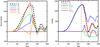 |
Fig. A.1 Left panel: relative magnetic helicity
( |
Acknowledgments
G.V. thanks the Scientific Council of the Observatoire de Paris for supporting his stay during which this work has been initiated, and acknowledges the support of the Leverhulme Trust Research Project Grant 2014-051, and funding from the European Com missions Seventh Framework Programme under the grant agreements no. 284461 (eHEROES project). K.D. acknowledges funding from the Computational and Information Systems Laboratory, the High Altitude Observatory, and support from the Air Force Office of Scientific Research under award FA9550-15-1-0030. The National Center for Atmospheric Research is sponsored by the National Science Foundation. G.V. and E.P. thanks ISSI, its members and the participants of the ISSI international team on Magnetic Helicity estimations in models and observations of the solar magnetic field, where this work has been discussed and commented on. The numerical simulations presented in this article have been performed thanks to the HPC resources of CINES, granted under the allocations 2014–046331 by GENCI (Grand Équipement National de Calcul Intensif).
References
- Alexakis, A., Mininni, P. D., & Pouquet, A. 2006, ApJ, 640, 335 [NASA ADS] [CrossRef] [Google Scholar]
- Antiochos, S. K., & DeVore, C. R. 1999, Magnetic Helicity in Space and Laboratory Plasmas: Geophysical Monograph 111, ed. M. R. Brown, 187 [Google Scholar]
- Barnes, C. W., Fernández, J. C., Henins, I., et al. 1986, Phys. Fluids, 29, 3415 [NASA ADS] [CrossRef] [Google Scholar]
- Berger, M. A. 1984, Geophys. Astrophys. Fluid Dyn., 30, 79 [NASA ADS] [CrossRef] [Google Scholar]
- Berger, M. A. 2003, Advances in Nonlinear Dynamics, eds. A. Ferriz-Mas, & M. Núñez (London: Taylor and Francis Group), 345 [Google Scholar]
- Berger, M. A., & Field, G. B. 1984, J. Fluid Mech., 147, 133 [NASA ADS] [CrossRef] [Google Scholar]
- Biskamp, D., & Müller, W.-C. 1999, Phys. Rev. Lett., 83, 2195 [NASA ADS] [CrossRef] [Google Scholar]
- Blackman, E. G., & Hubbard, A. 2014, MNRAS, 442, 1040 [NASA ADS] [CrossRef] [Google Scholar]
- Brandenburg, A., & Subramanian, K. 2005, Phys. Rep., 417, 1 [NASA ADS] [CrossRef] [Google Scholar]
- Candelaresi, S. 2012, Ph.D. Thesis, 126 [Google Scholar]
- Christensson, M., Hindmarsh, M., & Brandenburg, A. 2005, Astron. Nachr., 326, 393 [NASA ADS] [CrossRef] [Google Scholar]
- Del Sordo, F., Candelaresi, S., & Brandenburg, A. 2010, Phys. Rev. E, 81, 036401 [NASA ADS] [CrossRef] [Google Scholar]
- Démoulin, P. 2007, Adv. Space Res., 39, 1674 [Google Scholar]
- Démoulin, P., & Berger, M. A. 2003, Sol. Phys., 215, 203 [NASA ADS] [CrossRef] [Google Scholar]
- Démoulin, P., & Pariat, E. 2009, Adv. Space Res., 43, 1013 [NASA ADS] [CrossRef] [Google Scholar]
- DeVore, C. R. 1991, J. Comput. Phys., 92, 142 [NASA ADS] [CrossRef] [MathSciNet] [Google Scholar]
- DeVore, C. R. 2000, ApJ, 539, 944 [NASA ADS] [CrossRef] [Google Scholar]
- Elsasser, W. M. 1956, Rev. Mod. Phys., 28, 135 [NASA ADS] [CrossRef] [Google Scholar]
- Finn, J. H., & Antonsen, T. M. J. 1985, Comments on Plasma Physics and Controlled Fusion, 9, 111 [Google Scholar]
- Frisch, U., Pouquet, A., Leorat, J., & Mazure, A. 1975, J. Fluid Mech., 68, 769 [NASA ADS] [CrossRef] [Google Scholar]
- Gray, T., Lukin, V. S., Brown, M. R., & Cothran, C. D. 2010, Phys. Plasmas, 17, 102106 [NASA ADS] [CrossRef] [Google Scholar]
- Heidbrink, W. W., & Dang, T. H. 2000, Plasma Physics and Controlled Fusion, 42, L31 [NASA ADS] [CrossRef] [Google Scholar]
- Heyvaerts, J., & Priest, E. R. 1984, A&A, 137, 63 [NASA ADS] [Google Scholar]
- Ji, H. 1999, Magnetic Helicity in Space and Laboratory Plasmas, 111, 167 [CrossRef] [Google Scholar]
- Ji, H., Prager, S. C., & Sarff, J. S. 1995, Phys. Rev. Lett., 74, 2945 [NASA ADS] [CrossRef] [Google Scholar]
- Karpen, J. T., Antiochos, S. K., & DeVore, C. R. 2012, ApJ, 760, 81 [NASA ADS] [CrossRef] [Google Scholar]
- Knizhnik, K. J., Antiochos, S. K., & DeVore, C. R. 2015, Joint American Astronomical Society/American Geophysical Union Triennial Earth-Sun Summit, 1, 11305 [Google Scholar]
- Kusano, K., Maeshiro, T., Yokoyama, T., & Sakurai, T. 2004, ApJ, 610, 537 [NASA ADS] [CrossRef] [Google Scholar]
- Linton, M. G., & Antiochos, S. K. 2002, ApJ, 581, 703 [NASA ADS] [CrossRef] [Google Scholar]
- Linton, M. G., & Antiochos, S. K. 2005, ApJ, 625, 506 [NASA ADS] [CrossRef] [Google Scholar]
- Linton, M. G., Dahlburg, R. B., & Antiochos, S. K. 2001, ApJ, 553, 905 [Google Scholar]
- Liu, Y., Hoeksema, J. T., Bobra, M., et al. 2014a, ApJ, 785, 13 [NASA ADS] [CrossRef] [Google Scholar]
- Liu, Y., Hoeksema, J. T., & Sun, X. 2014b, ApJ, 783, L1 [NASA ADS] [CrossRef] [Google Scholar]
- Liu, Y., Zhao, J., & Schuck, P. W. 2013, Sol. Phys., 287, 279 [NASA ADS] [CrossRef] [Google Scholar]
- Low, B. C. 1996, Sol. Phys., 167, 217 [Google Scholar]
- MacNeice, P., Olson, K. M., Mobarry, C., de Fainchtein, R., & Packer, C. 2000, Comput. Phys. Comm., 126, 330 [Google Scholar]
- Mandrini, C. H., Pohjolainen, S., Dasso, S., et al. 2005, A&A, 434, 725 [NASA ADS] [CrossRef] [EDP Sciences] [Google Scholar]
- Mininni, P. D. 2007, Phys. Rev. E, 76, 26316 [NASA ADS] [CrossRef] [Google Scholar]
- Moffatt, H. K. 1969, J. Fluid Mech., 35, 117 [NASA ADS] [CrossRef] [Google Scholar]
- Nakwacki, M. S., Dasso, S., Démoulin, P., Mandrini, C. H., & Gulisano, A. M. 2011, A&A, 535, A52 [NASA ADS] [CrossRef] [EDP Sciences] [Google Scholar]
- Pariat, E., Démoulin, P., & Berger, M. A. 2005, A&A, 439, 1191 [NASA ADS] [CrossRef] [EDP Sciences] [Google Scholar]
- Pariat, E., Antiochos, S. K., & DeVore, C. R. 2009, ApJ, 691, 61 [NASA ADS] [CrossRef] [Google Scholar]
- Pariat, E., Antiochos, S. K., & DeVore, C. R. 2010, ApJ, 714, 1762 [NASA ADS] [CrossRef] [Google Scholar]
- Pariat, E., Dalmasse, K., DeVore, C. R., Antiochos, S. K., & Karpen, J. T. 2015, A&A, 573, A130 [NASA ADS] [CrossRef] [EDP Sciences] [Google Scholar]
- Patsourakos, S., Pariat, E., Vourlidas, A., Antiochos, S. K., & Wuelser, J. P. 2008, ApJ, 680, L73 [NASA ADS] [CrossRef] [Google Scholar]
- Pouquet, A., Frisch, U., & Leorat, J. 1976, J. Fluid Mech., 77, 321 [NASA ADS] [CrossRef] [Google Scholar]
- Prager, S. C. 1999, Magnetic Helicity in Space and Laboratory Plasmas, 111, 55 [CrossRef] [Google Scholar]
- Rachmeler, L. A., Pariat, E., DeForest, C. E., Antiochos, S. K., & Török, T. 2010, ApJ, 715, 1556 [NASA ADS] [CrossRef] [Google Scholar]
- Rudenko, G. V., & Myshyakov, I. I. 2011, Sol. Phys., 270, 165 [NASA ADS] [CrossRef] [Google Scholar]
- Russell, A. J. B., Yeates, A. R., Hornig, G., & Wilmot-Smith, A. L. 2015, Phys. Plasmas, 22, 032106 [NASA ADS] [CrossRef] [Google Scholar]
- Rust, D. M. 1994, Geophys. Res. Lett., 21, 241 [NASA ADS] [CrossRef] [Google Scholar]
- Stallard, B. W., Hooper, E. B., Woodruff, S., et al. 2003, Phys. Plasmas, 10, 2912 [NASA ADS] [CrossRef] [Google Scholar]
- Taylor, J. B. 1974, Phys. Rev. Lett., 33, 1139 [NASA ADS] [CrossRef] [Google Scholar]
- Taylor, J. B. 1986, Rev. Mod. Phys., 58, 741 [NASA ADS] [CrossRef] [Google Scholar]
- Thalmann, J. K., Inhester, B., & Wiegelmann, T. 2011, Sol. Phys., 272, 243 [NASA ADS] [CrossRef] [Google Scholar]
- Valori, G., Démoulin, P., & Pariat, E. 2012, Sol. Phys., 278, 347 [NASA ADS] [CrossRef] [EDP Sciences] [Google Scholar]
- Valori, G., Démoulin, P., Pariat, E., & Masson, S. 2013, A&A, 553, 38 [Google Scholar]
- Woltjer, L. 1958, in PNAS, 44, 489 [Google Scholar]
- Yamada, M. 1999, Magnetic Helicity in Space and Laboratory Plasmas, 111, 129 [CrossRef] [Google Scholar]
- Yang, S., Büchner, J., Santos, J. C., & Zhang, H. Q. 2013, Sol. Phys., 283, 369 [NASA ADS] [CrossRef] [Google Scholar]
- Zhang, Y., Kitai, R., & Takizawa, K. 2012, ApJ, 751, 85 [NASA ADS] [CrossRef] [Google Scholar]
- Zhao, L., DeVore, C. R., Antiochos, S. K., & Zurbuchen, T. H. 2015, ApJ, 805, 61 [Google Scholar]
All Figures
|
Fig. 1 Snapshots of the magnetic field evolution during the generation of the jet. The red field lines are initially closed. The green and white field lines are initially open. All the field lines are plotted from fixed footpoints. The red and white field lines are regularly plotted along a circle of constant radius, while the green field lines are plotted along the x-axis. At t = 900 the system is in its pre-eruption stage. It is close to the maximum of energy and helicity. All the helicity is stored in the close domain. At t = 1000 the system is erupting. Numerous field lines have changed their connectivity, as can be observed from the open red field lines and the closed white field lines. Helicity is ejected upward along newly opened reconnected field lines. At t = 1500 the system is slowly relaxing to its final stage. |
| In the text | |
|
Fig. 2 Top panel: time evolution of the different magnetic energies relative to their respective initial values: total ( |
| In the text | |
|
Fig. 3 Comparison of the helicity variation rate and the helicity flux computed in the practical DeVore gauge. The helicity variation rate ( |
| In the text | |
|
Fig. 4 Total helicity flux, Ftot (Eq. (30)), and the terms compositing it, Eqs. (26)−(29), through the different boundaries computed in the practical DeVore gauge. a) Ftot; b) Fφ; c) FAAp; d) FBn; and e) FVn. In each plot the dark line corresponds to the sum of the flux through all the boundaries, while the color lines correspond to a flux through a particular boundary (purple and blue: left and right x sides, green and orange: front and back y sides; yellow and red: bottom and top z sides). |
| In the text | |
|
Fig. 5 Difference between the helicity variation rate and the boundary helicity flux computed in the practical DeVore gauge. The relative helicity conservation criterion Cr (red line, Eq. (41)) and the magnetic helicity dissipation criterion Cm (blue line, Eq. (42)) are plotted relative to the helicity variation rate ( |
| In the text | |
|
Fig. 6 Left panel: comparison of the evolution of magnetic energy ( |
| In the text | |
|
Fig. 7 Left panel: evolution of the magnetic helicity computed with the practical DeVore method (dashed line) and with the DeVore-Coulomb method (red line). Their difference is plotted with an orange line (cf. right axis). Right panel: volume magnetic helicity ( |
| In the text | |
|
Fig. 8 Left panel: comparison of the helicity variation rate and the helicity flux integrated through the six boundaries of the domain in the DeVore-Coulomb case. The plotted curves are similar as in Fig. 3. Right panel: magnetic helicity dissipation criterion Cm, Eq. (42), plotted for the practical DeVore (black line) and the DeVore-Coulomb (red line) methods. The inset shows ϵCm, Eq. (44), with the same color convention. |
| In the text | |
|
Fig. 9
|
| In the text | |
|
Fig. A.1 Left panel: relative magnetic helicity
( |
| In the text | |
Current usage metrics show cumulative count of Article Views (full-text article views including HTML views, PDF and ePub downloads, according to the available data) and Abstracts Views on Vision4Press platform.
Data correspond to usage on the plateform after 2015. The current usage metrics is available 48-96 hours after online publication and is updated daily on week days.
Initial download of the metrics may take a while.