© ESO, 2015

1. Introduction

For most astrophysical plasmas the viscosity and current dissipation (resistivity) are negligibly small, that is, astrophysical plasmas are nearly ideal, almost dissipationless, and hence, for relevant processes and scales, the characteristic Reynolds and Lundquist numbers are very large. This requires specific approaches to correctly take into account turbulence and different types of ideal and non-ideal interactions in the plasma flows such as shock waves, dynamo action, and magnetic reconnection (Birn & Priest 2007). Fortunately, improvements in computer technology as well as the development of efficient algorithms allow increasingly realistic numerical simulations of the underlying space plasma processes (Büchner et al. 2003). For the proper numerical description of nearly dissipationless astrophysical plasmas, for example, of magnetic reconnection (Büchner 2007a) and dynamo action, one needs to employ schemes with negligible numerical diffusion for magnetohydrodynamical (MHD) as well as kinetic plasma descriptions (Elkina & Büchner 2006). The schemes should be as simple as possible so that they can run quickly and efficiently. Moreover, to ensure flexibility concerning the particular physics problem under consideration, they should allow an easy modification of initial and boundary conditions as well as the simple addition and adjustment of physics modules. For this purpose, the serial second-order-accurate MHD simulation code LINMOD3D had been developed, to name just one. It was successfully applied to study the magnetic coupling between the solar photosphere and corona based on multiwavelength observations (Büchner et al. 2004b), to investigate the heating of the transition region of the solar atmosphere (Büchner et al. 2004a), and the acceleration of the fast solar wind by magnetic reconnection (Büchner & Nikutowski 2005a). It was also used to physically consistently describe the evolution of the solar chromospheric and coronal magnetic fields (Büchner & Nikutowski 2005b) and to compare solar reconnection with spacecraft telescope observations (Büchner 2007b), the electric currents around EUV bright points (Santos et al. 2008a), the role of magnetic null points in the solar corona (Santos et al. 2011b), and the triggering of flare eruptions (Santos et al. 2011a). Other typical applications of LINMOD3D were the investigation of the relative importance of compressional heating and current dissipation for the formation of coronal X-ray bright points (Javadi et al. 2011) and of the role of the helicity evolution for the dynamics of active regions (Yang et al. 2013). To investigate stronger magnetic field gradients in larger regions of the solar atmosphere, however, an enhanced spatial resolution is required. To a certain degree this was possible using the OpenMP parallelized code MPSCORONA3D, which can be run on large shared-memory parallel computing resources, to investigate the influence of the resistivity model on the solar coronal heating (Adamson et al. 2013), for instance.

To simulate further challenging problems, like the development and feedback of turbulence, for high-resolution simulations of large spatial domains, for the investigation of turbulent astrophysical plasmas with very large Reynolds numbers, for the consideration of subgrid-scale turbulence for large scale plasma phenomena, one needs to be able to use a much larger number of CPU cores than shared memory systems can provide, however. Hence, message passing interface (MPI) parallelized MHD codes such as ATHENA¹, BATS-R-US², BIFROST, ENZO³ or PENCIL⁴ have to be used; these codes run on distributed memory computers. The PENCIL code is accurate to sixth order in space and to third order in time. It uses centered spatial derivatives and a Runge-Kutta time-integration scheme. ENZO is a hybrid (MHD + N-body) code with adaptive mesh refinement, which uses a third-order piecewise parabolic method (Colella & Woodward 1984) with a two-shock approximate Riemann solver. ATHENA allows a static mesh refinement, implementing a higher order scheme and using a Godunov method on several different grid geometries (Cartesian, cylindrical). It employs third-order cell reconstructions and a Roe solver, Riemann solvers, and a split corner-transport upwind scheme (Colella 1990; Stone et al. 2008) with a constrained-transport method (Evans & Hawley 1988; Stone & Gardiner 2009). The BIFROST code is accurate to sixth order in space and to third order in time (Gudiksen et al. 2011). The code BATS-R-US solves the 3D MHD equations in finite-volume form using numerical methods related to Roe’s approximate Riemann solver. It uses an adaptive grid composed of rectangular blocks arranged in varying degrees of spatial refinement levels. We note that all these codes are of an accuracy higher than second order. As a result, every time step is numerically expensive and changes or modifications of initial and boundary conditions, for instance, require quite some effort. Conversely, second-order-accurate schemes are based on simpler numerics and efficient solvers. They are generally far easier to implement and modify, different types of initial and boundary conditions are parallelized, for example. On modern computer architectures the desired numerical accuracy can rather easily and computationally cheaply be achieved by enhancing the grid resolution. This motivated us to base our new code GOEMHD3 on a simple second-order-accurate scheme that is relatively straightforward to implement and parallelize, which facilitates modification and extension. GOEMHD3 runs quickly and efficiently on different distributed-memory computers from standard PC clusters to high-performance-computing (HPC) systems like the Hydra cluster of the Max Planck Society at the computing center (RZG) in Garching, Germany. To demonstrate the reach and limits of the code, GOEMHD3 was tested on standard problems and by simulating the response of the strongly height-stratified solar atmosphere based on photospheric observations using a large number of CPU cores. In Sect. 2 we describe the basic equations that are solved by the code (Sect. 2.1), together with their discretization and numerical implementation (Sect. 2.2). In Sect. 2.3 we describe the hybrid MPI-OpenMP parallelization of GOEMHD3. The performance of the code was tested with respect to different ideal and non-ideal plasma processes (Sect. 3). All tests were carried out using the same 3D code. For quasi-2D simulations the number of grid points in the invariant direction was reduced to four, the minimum value required by the discretization scheme. Section 3.1 presents a test of the hydrodynamic part of the code by simulating the well-posed problem of a Kelvin-Helmholtz velocity shear instability using the methodology developed by McNally et al. (2012) because it was also applied to test higher-order codes such as PENCIL, ATHENA, and ENZO. In Sect. 3.2 the ideal MHD limit is tested by simulating vortices according to Orszag & Tang (1979). In the past, Kelvin-Helmholtz instability and Orszag-Tang vortex tests have also been used to verify total-variation-diminishing schemes (Ryu et al. 1995). The possibility of numerical oscillations caused by the finite-difference discretization was investigated as in Wu (2007). To verify the explicit consideration of dissipative processes by GOEMHD3, a current decay test was performed by suppressing other terms in the equations (Sect. 3.3). The effective numerical dissipation rate of the new code was assessed by a set of 1D Harris-like current sheet (e.g., Kliem et al. 2000) simulations (Sect. 3.4) and by a fully 3D application with solar-corona physics (Sect. 4.5).Section 4 presents an application of GOEMHD3 to the evolution of the solar corona in response to changing conditions at the lower boundary according to the photospheric plasma and magnetic field evolution, and we document the computational performance of the code. The paper is summarized and conclusions for the use of GOEMHD3 are drawn in Sect. 5.

2. Basic equations and numerical implementation

2.1. Resistive MHD equations

For a compressible, isotropic plasma, the resistive MHD equations in dimensionless form read $\begin{array}{ccc}& & \frac{\mathit{\partial \rho }}{\mathit{\partial t}}\mathrm{+}\mathrm{\nabla }\mathrm{·}\mathrm{\left(}\mathit{\rho }{u}\mathrm{\right)}\mathrm{=}\mathit{\chi }{\mathrm{\nabla }}^{\mathrm{2}}\mathit{\rho }\\ & & \frac{\mathit{\partial }\mathrm{\left(}\mathit{\rho }{u}\mathrm{\right)}}{\mathit{\partial t}}\mathrm{+}\mathrm{\nabla }\mathrm{·}\left[\mathit{\rho }{u}{u}\mathrm{+}\frac{\mathrm{1}}{\mathrm{2}}\mathrm{(}\mathit{p}\mathrm{+}{\mathit{B}}^{\mathrm{2}}\mathrm{)}{I}\mathrm{-}{B}{B}\right]\mathrm{=}\mathrm{-}\mathit{\nu \rho }\mathrm{(}{u}\mathrm{-}{{u}}_{\mathrm{0}}\mathrm{)}\mathrm{+}\mathit{\chi }{\mathrm{\nabla }}^{\mathrm{2}}\mathit{\rho }{u}\\ & & \\ & & \end{array}$where the symbols ρ, u, h, and B denote the primary variables, density, velocity, specific entropy of the plasma, and the magnetic field, respectively. The symbol I is the 3 × 3 identity matrix. The resistivity of the plasma is given by η and the collision coefficient ν accounts for the coupling of the plasma to a neutral gas moved around with a velocity u₀. The system of equations is closed by an equation of state. The entropy h is expressed via the scalar pressure p as p = 2h^γ. When the entropy is used as a variable instead of the internal energy (here adiabatic conditions are assumed, i.e., a ratio of the specific heats γ = 5/3), then Eq. (4) shows that in contrast to the internal energy, the entropy is conserved in the absence of Joule and viscous heating. Ampere’s law j = ∇ × B allows eliminating the current density j. The terms proportional to χ in Eqs. (1), (2), and (4) are added for technical reasons, as explained in the next section (Sect. 2.2).

The variables are rendered dimensionless by choosing typical values for a length scale L₀, a normalizing density ρ₀, and a magnetic field strength B₀. To normalize the remaining variables and parameters, the following definitions are used: ${\mathit{p}}_{\mathrm{0}}\mathrm{=}\frac{{\mathit{B}}_{\mathrm{0}}^{\mathrm{2}}}{\mathrm{2}{\mathit{\mu }}_{\mathrm{0}}}$ for a typical (magnetic) pressure, ${\mathit{u}}_{\mathrm{A}\mathrm{0}}\mathrm{=}\frac{{\mathit{B}}_{\mathrm{0}}}{\sqrt{{\mathit{\mu }}_{\mathrm{0}}{\mathit{\rho }}_{\mathrm{0}}}}$ for a typical (Alfvén) velocity, and τ₀ for the Alfvén crossing time over a distance L₀, that is, ${\mathit{\tau }}_{\mathrm{A}\mathrm{0}}\mathrm{=}\frac{{\mathit{L}}_{\mathrm{0}}}{{\mathit{u}}_{\mathrm{A}\mathrm{0}}}$. The current density is normalized by ${\mathit{j}}_{\mathrm{0}}\mathrm{=}\frac{{\mathit{B}}_{\mathrm{0}}}{{\mathit{\mu }}_{\mathrm{0}}{\mathit{L}}_{\mathrm{0}}}$, the resistivity by η₀ = μ₀L₀u_A0, and the energy by ${\mathit{E}}_{\mathrm{0}}\mathrm{=}{\mathit{B}}_{\mathrm{0}}^{\mathrm{2}}{\mathit{L}}_{\mathrm{0}}^{\mathrm{2}}\mathit{/}{\mathit{\mu }}_{\mathrm{0}}$. For simulations of the solar atmosphere, typical numerical values are L₀ = 5000 km, ρ₀ = 2 × 10¹⁵ m^-3 and B₀ = 10^-3 T, which yields p₀ = 0.7958 Pa, u_A0 = 487.7 kms^-1, τ_A0 = 10.25 s, j₀ = 1.59 × 10^-4 Am^-2, η₀ = 3.06 × 10⁶ Ω.m, and W₀ = 1.99 × 10¹³ J for the normalizing energy.

2.2. Numerical implementation

The resistive MHD equations (Eqs. (1)–(4)) are discretized on a 3D Cartesian grid employing a combination of a time-explicit leap-frog, a Lax, and a DuFort-Frankel finite-difference scheme (see Press et al. 2007). For the conservative, homogeneous part of the MHD equations, we adopted a second-order accurate leap-frog discretization scheme 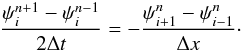$\begin{array}{ccc}\frac{{\mathit{\psi }}_{\mathit{i}}^{\mathit{n}\mathrm{+}\mathrm{1}}\mathrm{-}{\mathit{\psi }}_{\mathit{i}}^{\mathit{n}\mathrm{-}\mathrm{1}}}{\mathrm{2}\mathrm{\Delta }\mathit{t}}\mathrm{=}\mathrm{-}\frac{{\mathit{\psi }}_{\mathit{i}\mathrm{+}\mathrm{1}}^{\mathit{n}}\mathrm{-}{\mathit{\psi }}_{\mathit{i}\mathrm{-}\mathrm{1}}^{\mathit{n}}}{\mathrm{\Delta }\mathit{x}}\mathrm{·}& & \end{array}$(5)A first-order Lax method is used to start the integration from initial conditions, that is, to compute ψⁿ from the given initial values ψⁿ⁻¹, or upon a change of the time step Δt (see below).

The advantage of the leap-frog scheme lies in its low numerical dissipation – in the derivation of the scheme all even derivative terms cancel out in the expansion, and a von Neumann stability analysis shows that there is no amplitude dissipation for the linearized system of MHD equations. The full nonlinear system in principle exhibits finite dissipation rates, corresponding to additional nonlinear terms in the von Neumann stability analysis. As we show in Sects. 3.4 and 4.5, the effective numerical dissipation rates found with GOEMHD3 are sufficiently low to enable simulations of almost ideal dissipationless magneto-fluids with very high Reynolds number (Re ~ 10¹⁰).

The disadvantage of the leap-frog scheme is that it is prone to generating oscillations. When such numerical oscillations arise, they must be damped by a locally switched-on diffusivity, for example, which prevents a steepening of gradients beyond those resolved by the grid. This also prevents mesh-drift instabilities of staggered leap-frog schemes that arise because odd and even mesh points are decoupled (see, e.g., Press et al. 2007 and Yee 1966).

This general oscillation-damping diffusion is explicitely introduced via terms proportional to χ∇²ρ, χ∇²ρu, and χ∇²h in the right-hand sides of Eqs. (1), (2), and (4). Finite χ are switched on only when necessary for damping, as explained below. Hence, although a leap-frog scheme is by construction dissipationless (at least in the linear regime), we combined it with an explicit, externally controllable diffusion necessary to avoid oscillations. This in the end makes the scheme dissipative, but in a controlled way. To maintain second-order accuracy, the dissipative terms are discretized by a DuFort-Frankel scheme, which is also used to discretize the diffusion term in the induction Eq. (3): $\begin{array}{ccc}{\mathit{\psi }}_{\mathit{i}}^{\mathit{n}\mathrm{+}\mathrm{1}}\mathrm{=}{\mathit{\psi }}_{\mathit{i}}^{\mathit{n}\mathrm{-}\mathrm{1}}\mathrm{+}\mathrm{2}\mathrm{\Delta }\mathit{t}\left[{\mathit{w}}_{\mathrm{1}}{\mathit{\psi }}_{\mathit{i}\mathrm{-}\mathrm{1}}^{\mathit{n}}\mathrm{+}{\mathit{w}}_{\mathrm{3}}{\mathit{\psi }}_{\mathit{i}\mathrm{+}\mathrm{1}}^{\mathit{n}}\mathrm{+}\frac{\mathrm{1}}{\mathrm{2}}{\mathit{w}}_{\mathrm{2}}\mathrm{(}{\mathit{\psi }}_{\mathit{i}}^{\mathit{n}\mathrm{-}\mathrm{1}}\mathrm{+}{{\mathit{\psi }}_{\mathit{i}}^{\mathit{n}\mathrm{+}\mathrm{1}}}^{\mathrm{)}}\right]\mathit{.}& & \end{array}$(6)Here, ${\mathit{w}}_{\mathrm{1}}\mathrm{=}\frac{\mathrm{2}}{\mathrm{\Delta }{\mathit{x}}_{\mathit{l}}\mathrm{\Delta }\mathit{x}}$, ${\mathit{w}}_{\mathrm{2}}\mathrm{=}\frac{-2}{\mathrm{\Delta }{\mathit{x}}_{\mathit{l}}\mathrm{\Delta }{\mathit{x}}_{\mathit{r}}}$, and ${\mathit{w}}_{\mathrm{3}}\mathrm{=}\frac{\mathrm{2}}{\mathrm{\Delta }{\mathit{x}}_{\mathit{r}}\mathrm{\Delta }\mathit{x}}$ are the coefficients necessary for calculating the second-order derivatives on the nonequidistant mesh. The left derivative is denoted by Δx_l = x_i−x_i−1, the right by Δx_l = x_{i + 1}−x_i, and the total by Δx = Δx_l + Δx_r.

By combining the leap-frog (Eq. (5)) and the DuFort-Frankel (Eq. (6)) discretization schemes, we obtain $\begin{array}{ccc}{\mathit{\psi }}^{\mathit{n}\mathrm{+}\mathrm{1}}\mathrm{=}{\mathit{\psi }}^{\mathit{n}\mathrm{-}\mathrm{1}}\mathrm{+}\mathit{\lambda }\left[{\mathit{S}}^{\mathit{n}}\mathrm{+}\sum _{\mathit{i}}\left({\mathit{\chi }}_{\mathit{i}}{\mathit{H}}_{\mathit{i}}\mathrm{-}\mathrm{d}{\mathit{x}}_{\mathit{i}}{\mathit{F}}_{\mathit{i}}^{\mathit{n}}\right)\right]\mathit{,}& & \end{array}$(7)with the fluxes ${\mathit{F}}_{\mathit{i}}^{\mathit{n}}$ and source terms S_i$\begin{array}{ccc}{F}\mathrm{=}\left(\begin{array}{c}\\ \\ \\ \\ \end{array}\right)\mathit{,} {S}\mathrm{=}\left(\begin{array}{c}\\ \\ \\ \\ \end{array}\right)\mathit{.}& & \end{array}$(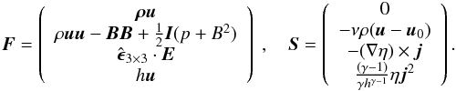8)The diffusion term is 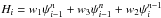${\mathit{H}}_{\mathit{i}}\mathrm{=}{\mathit{w}}_{\mathrm{1}}{\mathit{\psi }}_{\mathit{i}\mathrm{-}\mathrm{1}}^{\mathit{n}}\mathrm{+}{\mathit{w}}_{\mathrm{3}}{\mathit{\psi }}_{\mathit{i}\mathrm{-}\mathrm{1}}^{\mathit{n}}\mathrm{+}{\mathit{w}}_{\mathrm{2}}{\mathit{\psi }}_{\mathit{i}}^{\mathit{n}\mathrm{-}\mathrm{1}}$, where $\widehat{{ϵ}}{}_{\mathrm{3}\mathrm{\times }\mathrm{3}}$ is the permutation pseudo-tensor, E = −u × B is the convection electric field, and ψ represents any one of the plasma variables ρ, ρu, B, and h. Equation (7) further uses the abbreviations $\mathit{\lambda }\mathrm{=}\frac{\mathrm{d}\mathit{t}}{\mathrm{1}\mathrm{-}\frac{\mathrm{1}}{\mathrm{2}}\sum {\mathit{\chi }}_{\mathit{i}}{\mathit{w}}_{\mathrm{2}\mathit{,i}}}$, dt = 2Δt, d${\mathit{x}}_{\mathit{i}}\mathrm{=}\frac{\mathrm{1}}{\mathrm{\Delta }{\mathit{x}}_{\mathit{i}}}$, and the index i represents the x, y, and z directions.

Note that two terms of the source vector S are not treated exactly according to this scheme: as a result of the staggered nature of the leap-frog scheme, the values of h at time level n are not available in the pressure equation. Similarly, for the induction equation, the gradient of the resistivity is needed at time level n. While in the former case, hⁿ can simply be approximated by averaging over the neighboring grid points, now the gradient ∇ηⁿ is extrapolated from the previous time level n−1, assuming that the arising numerical error is small for a resistivity that is reasonably smoothed both in space and in time. The resistivity is smoothed in time if a time-dependent resistivity model is used. GOEMHD3 is meant to describe collisionless astrophysical plasmas of the solar corona, for instance, where resistivity is physically caused by micro-turbulence. Since it is not possible to describe kinetic processes like micro-turbulence in the framework of an MHD fluid-model, different types of switch-on resistivity models are implemented in GOEMHD3 to mimic a kinetic-scale current dissipation at the macro scales. The criteria controlling the switch-on of resistivity usually localize the resistivity increase. This allows reaching the observed magnetic reconnection rates, for example. Current dissipation is expected to be most prominent in regions of enhanced current densities where the use of smooth resistivity models is appropriate.

As noted before, the numerical oscillations are damped by switching on diffusion. As soon as the value of ψ exhibits two or more local extrema (either maxima or minima) in any of the three coordinate directions, the diffusion coefficient χ is given a finite value, as an example, we chose ≃10^-2, at the given grid point and its next neighbors. If at least two extrema are found, then the diffusion term is switched on locally in the corresponding direction. For this all directions (x,y and z) are considered separately.

For solar applications it is possible to start GOEMHD3 with initially force-free magnetic fields. These magnetic fields are obtained by a numerical extrapolation of the observed photospheric magnetic field. To improve the accuracy for strong initial magnetic fields, the current density is evaluated by calculating j = ∇ × (B−B_init), that is, for a field from which the initial magnetic field B_init is subtracted. This reduces the error arising from the discretization of the magnetic field. In this case, the current density is explicitly used to solve the momentum equation, which has the form $\begin{array}{ccc}\frac{\mathit{\partial \rho }{u}}{\mathit{\partial t}}\mathrm{+}\mathrm{\nabla }\mathrm{·}\left[\mathit{\rho }{u}{u}\mathrm{+}\frac{\mathrm{1}}{\mathrm{2}}\mathit{p}{I}\right]\mathrm{-}{j}\mathrm{\times }{B}\mathrm{=}\mathrm{-}\mathit{\nu \rho }\mathrm{(}{u}\mathrm{-}{{u}}_{\mathrm{0}}\mathrm{)}\mathrm{+}\mathit{\chi }{\mathrm{\nabla }}^{\mathrm{2}}\mathit{\rho }{u}\mathit{.}& & \end{array}$(9)For this case, GOEMHD3 can alternatively solve the momentum equation Eq. (9) instead of Eq. (2).

Time step control.

The time-explicit discretization entails a time-step limit according to the Courant-Friedrichs-Lewy (CFL) condition, which basically requires that during a time step no information is propagated beyond a single cell of the numerical grid. To this end, the minimum value of the sound, Alfvén, and fluid crossing times, and similarly for the resistive time scale, is determined for every grid cell, 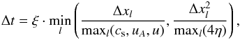$\begin{array}{ccc}\mathrm{\Delta }\mathit{t}\mathrm{=}\mathit{\xi }\mathrm{·}\underset{\mathit{l}}{\min }\left(\frac{\mathrm{\Delta }{\mathit{x}}_{\mathit{l}}}{{\max }_{\mathit{l}}\mathrm{\left(}{\mathit{c}}_{\mathrm{s}}\mathit{,}{\mathit{u}}_{\mathit{A}}\mathit{,u}\mathrm{\right)}}\mathit{,}\frac{\mathrm{\Delta }{\mathit{x}}_{\mathit{l}}^{\mathrm{2}}}{{\max }_{\mathit{l}}\mathrm{\left(}\mathrm{4}\mathit{\eta }\mathrm{\right)}}\right)\mathit{,}& & \end{array}$(10)with the local values of the sound speed, ${\mathit{c}}_{\mathrm{s}}\mathrm{=}\sqrt{\mathit{\gamma p}\mathit{/}\mathit{\rho }}$, the Alfvén speed, ${\mathit{u}}_{\mathit{A}}\mathrm{=}\sqrt{{{B}}^{\mathrm{2}}\mathit{/}\mathit{\rho }}$, and the macroscopic velocity u = | u | at the grid position l. Typically, a value of 0.2 is chosen for the constant safety factor ξ ∈ (0,1).

In our simulations the time step Δt was changed only after several (usually at least aboutten) time steps, which avoids interleaving a necessary Lax integration step too frequently and hence compromising the overall second-order accuracy of the leap-frog scheme. To prevent an unlimited decrease of the time step, limiting values of at least 10% of the initial values of the density and 1% of the entropy h, for example, and u< 3u_A were enforced. The values at the corresponding grid points were reset to the corresponding cut-off value, and the values at the surrounding grid points were smoothed by averaging over the neighboring grid points.

Divergence cleaning.

As a result of discretization errors, unphysical finite divergences of the magnetic field may arise. To remove such finite values of ∇B,weapplied the following cleaning method that solves a Poisson equation for the magnetic potential φ: 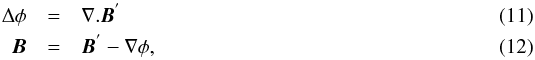$\begin{array}{ccc}\mathrm{\Delta }\mathit{\phi }& \mathrm{=}& \\ {B}& \mathrm{=}& {{B}}^{\mathrm{\prime }}\mathrm{-}\mathrm{\nabla }\mathit{\phi ,}\end{array}$where B′ is the magnetic field with a finite divergence, and B is the cleaned magnetic field. With central differences d_x = 1/(x_{i + 1}−x_i−1), and similarly for the other coordinate directions, which are suppressed here for brevity, the Poisson equation Eq. (11) is discretized as $\begin{array}{ccc}{\mathit{d}}_{\mathit{x}}\mathrm{(}{\mathit{d}}_{\mathit{x}\mathrm{-}\mathrm{1}}\mathrm{+}{\mathit{d}}_{\mathit{x}\mathrm{+}\mathrm{1}}\mathrm{)}\overline{\mathit{\phi }}\begin{array}{c}\mathit{k}\mathrm{+}\mathrm{1}\\ \mathit{i}\end{array}& \mathrm{=}& {\mathit{d}}_{\mathit{x}}\mathrm{(}{\mathit{B}}_{\mathit{x}\mathrm{+}\mathrm{1}}\mathrm{-}{\mathit{B}}_{\mathit{x}\mathrm{-}\mathrm{1}}\mathrm{)}\\ & & \end{array}$(13)and is solved with a simple fix-point iteration, where k denotes the iteration step. For faster convergence we used a standard relaxation method, $\begin{array}{ccc}{\mathit{\phi }}_{\mathit{i}}^{\mathit{k}\mathrm{+}\mathrm{1}}\mathrm{=}\mathit{\xi }\overline{\mathit{\phi }}\begin{array}{c}\mathit{k}\mathrm{+}\mathrm{1}\\ \mathit{i}\end{array}\mathrm{+}\mathrm{(}\mathrm{1}\mathrm{-}\mathit{\xi }\mathrm{)}{\mathit{\phi }}_{\mathit{i}}^{\mathit{k}}\mathit{,}& & \end{array}$(14)where the relaxation coefficient ξ depends on the iteration k as $\begin{array}{ccc}\mathit{\xi }\mathrm{=}\frac{\mathrm{1}}{\mathrm{4}}\left(\tanh \left(\frac{\mathrm{16}\mathit{k}}{{\mathit{k}}_{\max }}\mathrm{-}\mathrm{2}\right)\mathrm{+}\mathrm{1}\right)\mathrm{+}\frac{\mathrm{1}}{\mathrm{2}}\mathrm{·}& & \end{array}$(15)

2.3. Hybrid MPI-OpenMP parallelization

The time-explicit discretization scheme described above can be straightforwardly parallelized using a domain decomposition approach and introducing halo regions (ghost zones) of width 1, corresponding to an effective stencil length of 3 in each of the coordinate directions. Accordingly, only next-neighbor communication and a single global reduction operation (for computing the time step, cf. Eq. (10)) are necessary for exchanging data between the domains. To be specific, GOEMHD3 employs a 2D domain decomposition in the y-z plane with width-1 halo exchange, using the MPI. Within the individual pencil-shaped domains, a shared-memory parallelization is implemented using OpenMP. The hybrid MPI-OpenMP approach first integrates smoothly with the existing structure of the serial code, and second, thanks to a very efficient OpenMP parallelization within the domains, allows using a sufficiently large number of processor cores, given typical sizes of the numerical grid ranging between 256³ and 2048³ points. In addition, the hybrid parallelization helps to maximize the size (i.e., volume in physical space) of the individual MPI domains, and hence to minimize the surface-to-volume ratio. The latter translates into a lower communication-to-computation ratio and hence relatively shorter communication times, and the former accounts for longer MPI messages and hence decreases communication overhead (latency). Our parallelization assumes the individual MPI domains to be of equal size (but not necessarily with a quadratic cross section in the y-z plane). This greatly facilitates the technical handling of the extrapolations required by so-called line-symmetric side-boundary conditions (Otto et al. 2007), which are often employed in realistic solar corona simulations. As a side effect, this restriction a priori avoids load-imbalances due to an otherwise non-uniform distribution of the processor workload.

Overall, as we demonstrate below (cf. Sect. 4.3), GOEMHD3 achieves very good parallel efficiency over a wide range of processor counts and sizes of the numerical grid, with the hybrid parallelization outperforming a plain MPI-based strategy at high core counts.

3. Test problems

To assess the stability, the convergence properties, and the numerical accuracy of the new GOEMHD3 code, we simulated the standard test problems of the Kelvin-Helmholtz instability and the Orszag-Tang vortex, performed a test (Skála & Bárta 2012) of the resistive MHD properties of the code, estimated the effective numerical dissipation in the nonlinear regime using a Harris-like current sheet, and compared our results with numerical and analytical reference solutions. All tests are 2D problems in the space coordinates. To perform these 2D simulations with our 3D code, the x-direction was considered invariant, and the numerical grid in this direction covered four points (minimum required by the code).

3.1. Kelvin-Helmholtz instability

The properties of the hydrodynamic limit of the GOEMHD3 code were verified by simulating the nonlinear evolution of the Kelvin-Helmholtz instability (KHI) in two dimensions. This is a well-known standard test of numerical schemes that solve the equations of hydrodynamics (see, e.g., McNally et al. 2012). The KHI instability is caused by a velocity shear. At its nonlinear stage, it leads to the formation of large-scale vortices. The time evolution of the size and growth rate of the vortices can be followed and compared with reference solutions obtained by other numerical schemes. We verified GOEMHD3 by closely following McNally et al. (2012). These authors established a standard methodology for the KHI test and published and sent us the results of their fiducial reference solutions obtained using the PENCIL code of simulations for high-resolution grids with up to 4096² grid points. To avoid problems of resolving sharp discontinuities that arise in some numerical schemes, McNally et al. (2012) proposed a test setup with smooth initial conditions as introduced by Robertson et al. (2010). For the two spatial coordinates 0 <y< 1 and 0 <z< 1) the initial conditions are therefore $\begin{array}{ccc}\mathit{\zeta }\mathrm{=}\{\begin{array}{c}\\ & \\ & \\ & \\ & \end{array}\mathit{,}& & \end{array}$(16)where ζ either denotes the density ρ or the velocity u_y, and ζ_m = (ζ₁ + ζ₂)/2. To trigger the instability, a small perturbation u_z = 0.01sin(4πy) was imposed on the velocity in the z-direction, while the initial pressure was assumed to be uniform in space: p = 5. Periodic boundary conditions were imposed. According to the stability requirements of our code, we imposed diffusion quantified by a coefficient χ = 4 × 10^-5 in Eqs. (1), (2) and (4).

Figure 1 shows snapshots of the fluid density at time t = 2.5 as computed by GOEMHD3 using different numerical resolution ranging from 128² (panel a) to 1024² (panel d) grid points. The familiar Kelvin-Helmholtz patterns are clearly recognizable and compare qualitatively well with published structures (e.g., Robertson et al. 2010; Springel 2010). For lower resolutions we observe somewhat smoother edges of the primary Kelvin-Helmholtz instability, which is due to the higher effective numerical diffusivity caused by the smoothing scheme of GOEMHD3 (cf. Sect. 2). For higher resolutions of 512² (panel c) and 1024² (panel d), secondary billows develop in the primary billows. As McNally et al. (2012) pointed out, these secondary billows are artifacts caused by numerical grid noise.

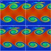Fig. 1 Color-coded mass density, ρ(y,z) at time t = 2.5 for the Kelvin-Helmholtz test problem. Panels a)–d) show the GOEMHD3 results for a numerical resolution of 1282, 2562, 5122, and 10242, respectively.

For a quantitative verification of GOEMHD3, we computed the time evolution of different variables introduced and defined by McNally et al. (2012). First we calculated the y-velocity mode amplitude A_y according to Eqs. (6) to (9) in McNally et al. (2012), its growth rate Ȧ_y, and the spatial maximum of the kinetic energy density of the motion in the y-direction (${\mathit{E}}_{\mathit{y}}\mathrm{=}\frac{\mathrm{1}}{\mathrm{2}}{\max }_{\mathit{y,z}}\mathrm{\left(}\mathit{\rho }{\mathit{u}}_{\mathit{y}}^{\mathrm{2}}\mathrm{\right)}$). We furthermore calculated the relative error by comparing GOEMHD3 results with those of the PENCIL reference code as obtained by McNally et al. (2012), who used the PENCIL code with a grid resolution of 4096² points. Finally, we calculated convergence quantities as defined by Roache (1998) for GOEMHD3. The results of these calculations are shown in Figs. 2–5.

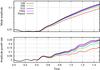Fig. 2 Time evolution of the y-velocity mode amplitude Ay (top panel) and of its growth rate Ȧy (bottom panel) in the course of the Kelvin-Helmholtz test. The results obtained by GOEMHD3 for different spatial resolutions are color-coded according to the legend. The black line corresponds to the result obtained by a PENCIL code run using a grid resolution of 40962 (McNally et al. 2012).

First, Fig. 2 shows that both the y-velocity mode amplitude A_y of the KHI (upper panel) and its growth rate (lower panel) converge well with increasing numerical resolution of GOEMHD3. They also agree very well overall with the reference solution obtained by using the PENCIL code. A closer look reveals, however, that while the initial evolution of A_y closely resembles the reference solution at high as well as at lower resolution, at later times a sufficiently high resolution of at least 512² is needed to match the PENCIL code results. The velocity mode growth rate Ȧ_y and the maximum of the kinetic energy density of the motion in the y-direction E_y behave similarly, as Fig. 3 shows. While GOEMHD3 initially follows the reference solution at all tested resolutions, at later times, GOEMHD3 results for lower resolution are slightly lower than the result obtained by the PENCIL code.

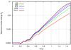Fig. 3 Time evolution of the highest kinetic energy density ${\mathit{E}}_{\mathit{y}}\mathrm{=}\frac{\mathrm{1}}{\mathrm{2}}{\max }_{\mathit{y,z}}\mathrm{\left(}\mathit{\rho }{\mathit{u}}_{\mathit{y}}^{\mathrm{2}}\mathrm{\right)}$ in the Kelvin-Helmholtz test. The results obtained by GOEMHD3 for different spatial resolutions are color-coded according to the legend. The black line corresponds to the result of a PENCIL code run using a grid resolution of 40962 (McNally et al. 2012).

Furthermore, we benchmarked GOEMHD3 by comparing it with the KHI test results obtained by the PENCIL code for the same initial conditions. We quantified the comparison by calculating the relative error | ε_A | of the mode amplitude ${\mathit{A}}_{\mathit{y}}^{\mathit{G}}$ obtained by GOEMHD3 with the corresponding values ${\mathit{A}}_{\mathit{y}}^{\mathit{P}}$ obtained by a 4096² grid points run of the PENCIL code for reference: 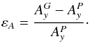$\begin{array}{ccc}{\mathit{\epsilon }}_{\mathit{A}}\mathrm{=}\frac{{\mathit{A}}_{\mathit{y}}^{\mathit{G}}\mathrm{-}{\mathit{A}}_{\mathit{y}}^{\mathit{P}}}{{\mathit{A}}_{\mathit{y}}^{\mathit{P}}}\mathrm{·}& & \end{array}$(17)For the whole time evolution of the KHI until t = 1.5 (the last value available from McNally et al. 2012), Fig. 4 shows the relative errors of the GOEMHD3 results compared to the benchmark solution that was obtained with the PENCIL code using 4096² grid points. The relative error decreases from 30% if GOEMHD3 is using 128² grid points to less than 4% if GOEMHD3 uses the same resolution of 4096² grid points as the PENCIL code. This is a very good result given that GOEMHD3 uses a numerically much less expensive second-order accurate scheme compared to the sixth-order scheme used in the PENCIL code.

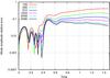Fig. 4 Time evolution of the relative error | εA | of the mode amplitude obtained for the Kelvin-Helmholtz test using GOEMHD3 compared to those obtained by the PENCIL code (McNally et al. 2012) for different numbers of grid points (color coded).

Now, we investigate how the mode amplitude converges with increasing mesh resolution and establish its uncertainty. The convergence assessment is based on the generalized Richardson extrapolation method, which allows extracting the convergence rate from simulations performed at three different grid resolutions with a constant refinement ratio (Roache 1998) $\begin{array}{ccc}\mathit{p}\mathrm{=}\ln \left(\frac{{\mathit{f}}_{\mathrm{3}}\mathrm{-}{\mathit{f}}_{\mathrm{2}}}{{\mathit{f}}_{\mathrm{2}}\mathrm{-}{\mathit{f}}_{\mathrm{1}}}\right)\mathit{/}\ln \mathrm{\left(}\mathit{r}\mathrm{\right)}\mathit{.}& & \end{array}$(18)Here, r = 2 is the mesh refinement ratio and f₁, f₂, and f₃ are the mode amplitudes for the fine, medium, and coarse mesh, respectively. From the convergence rate we can calculate the grid convergence index (GCI, Roache 1998), which indicates the uncertainty based on the grid convergence p. $\begin{array}{ccc}\mathit{GCI}\mathrm{=}{\mathit{F}}_{\mathrm{s}}\frac{\mathrm{\left|}\mathit{\epsilon }\mathrm{\right|}}{{\mathit{r}}^{\mathit{p}}\mathrm{-}\mathrm{1}}\mathit{,}& & \end{array}$(19)where ε = (f₂−f₁) /f₁ is a relative error and F_s = 1.25 is a safety factor. Following (Roache 1998), we used this value for grid convergence studies that compare three or more different resolutions. Figure 5 shows the time evolution of the grid convergence rate for the mode amplitude (upper panel) and the GCI corresponding to the finest resolution (lower panel). The convergence order of the GOEMHD3 runs appeared to be in the range (0.8−1.5). A convergence order p of about 1.5 for GOEMHD3, a second-order accurate code, is a very good result compared to convergence orders of about 2 obtained by higher (e.g., sixth-) order accurate schemes like PENCIL. At the same time, the mode amplitude uncertainty GCI for the highest resolution always remains lower than 0.008.

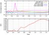Fig. 5 Time evolution of the grid convergence rate (top panel) of the mode amplitude in dependence on the spatial resolution given in the legend and of the grid convergence index GCI (bottom panel) of the mode amplitude uncertainty for the highest resolution.

The differences between the results obtained by GOEMHD3 and PENCIL at later times originate from the different role of diffusivity in the codes. While the leap-frog scheme implemented in GOEMHD3 is intrinsically not diffusive, it initially does not switch on diffusion either because no strong gradients are present, which would cause numerical oscillations. Hence the initial (linear) phase of the Kelvin-Helmholtz instability is well described by GOEMHD3 since it does not need additional smoothing at this stage. However, secondary billows develop earlier in the GOEMHD3 KHI test simulation than in PENCIL code simulations (see Fig. 1 and also Fig. 12 of McNally et al. 2012). This is due to the explicit diffusion that is switched on by the GOEMHD3 code when steep gradients have to be smoothed that develop during the turbulent phase of the KHI. As a result, GOEMHD3 initially, when it is still not diffusive at all, reveals the same Kelvin-Helmholtz instability growth even though is only second-order accurate. Later, however, at the nonlinear stage of the KHI, the explicit diffusion used in GOEMHD3 for smoothing exceeds the diffusion level of the sixth-order accurate PENCIL code.

3.2. Orszag-Tang test

The ideal-MHD limit of the GOEMHD3 code was tested by simulating an Orszag-Tang vortex setup in two dimensions (Orszag & Tang 1979). The test starts with an initially periodic velocity and magnetic fields, a constant mass density, and a pressure distribution given by 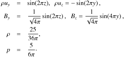$\begin{array}{ccc}\mathit{\rho }{\mathit{u}}_{\mathit{y}}& \mathrm{=}& \sin \mathrm{\left(}\mathrm{2}\mathit{\pi z}\mathrm{\right)}\mathit{,\rho }{\mathit{u}}_{\mathit{z}}\mathrm{=}\mathrm{-}\sin \mathrm{\left(}\mathrm{2}\mathit{\pi y}\mathrm{\right)}\hspace{0.17em}\mathit{,}\\ {\mathit{B}}_{\mathit{y}}& \mathrm{=}& \frac{\mathrm{1}}{\sqrt{\mathrm{4}\mathit{\pi }}}\sin \mathrm{\left(}\mathrm{2}\mathit{\pi z}\mathrm{\right)}\hspace{0.17em}\mathit{,}{\mathit{B}}_{\mathit{z}}\mathrm{=}\frac{\mathrm{1}}{\sqrt{\mathrm{4}\mathit{\pi }}}\sin \mathrm{\left(}\mathrm{4}\mathit{\pi y}\mathrm{\right)}\hspace{0.17em}\mathit{,}\\ \mathit{\rho }& \mathrm{=}& \frac{\mathrm{25}}{\mathrm{36}\mathit{\pi }}\mathit{,}\\ \mathit{p}& \mathrm{=}& \frac{\mathrm{5}}{\mathrm{6}\mathit{\pi }}\mathrm{·}\end{array}$(20)Hence both the velocity and magnetic fields contain X-points, where the fields vanish. In the y-direction the modal structure of the magnetic field differs from the velocity field structure. The simulation box size is [− 0.5,0.5] × [−0.5,0.5]. All boundary conditions are periodic. The coefficients χ of the smoothing diffusion terms are chosen to be 2 × 10^-4, 1 × 10^-4, 5 × 10^-5, and 2 × 10^-5 for meshes with 128², 256², 512², and 1024² grid points, respectively. As expected, GOEMHD3 reproduces purely growing vortices including sharp gradients, structures, and a dynamics that resembles the results obtained by Ryu et al. (1995) and Dai & Woodward (1998). To show an example, Fig. 6 depicts the mass density distribution at t = 0.25. Panels a–d of Fig. 6 correspond to mesh resolutions of 128², 256², 512², and 1024² grid points, respectively. Low-density regions are color-coded in blue, higher density values are plotted in red. Similar structures containing sharp gradients (shocks) were obtained also by ATHENA 4.2, for instance⁵, and by our least-squares finite element code (Skála & Bárta 2012). Note that, owing to its flux conservative discretization scheme, GOEMHD3 is able to accurately reproduce the position of shock fronts (cf. Fig. 7).

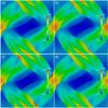Fig. 6 Mass density distribution obtained at t = 0.25 for the 2D Orszag-Tang test. Panels a)–d) correspond to a mesh resolution of 1282, 2562, 5122, and 10242 grid points, respectively.

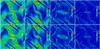Fig. 7 Thermal plasma pressure (panels a), e)), magnetic pressure (panels b), f)), vorticity ∇ × u (panels c), g)) and current density ∇ × B (panels d), h)) obtained for the 2D Orszag-Tang test by GOEMHD3 (top row) and ATHENA 4.2 (bottom row) for a grid resolution of 2562. t = 0.5.

The convergence properties of GOEMHD3 are illustrated by calculating the relative difference ε_ρ = (ρ₂−ρ₁) /ρ₁ of the spatial distribution of the mass density obtained by comparing the mass densities derived from runs with lower and higher mesh resolution. Here ρ₁ corresponds to the mass density distribution obtained for the higher mesh resolution and ρ₂ to the coarser grid. In particular, Fig. 8 shows the spatial distribution of the relative differences obtained at t = 0.5 for runs with doubled numbers of grid points – from 128² to 256², from 256² to 512², and from 512² to 1024² in panels a) to c), respectively. Figure 8 shows that the largest relative differences ε_ρ of the mass density are localized in regions of strong gradients (shock fronts), while they do not extend into regions of smooth flows.

Fig. 8 Spatial distribution of the relative difference | ερ | of the mass density obtained by GOEMHD3 simulating the Orszag-Tang vortex problem comparing the results for three different mesh resolutions of a) 1282–2562; b) 2562–5122; and c) 5122–10242 grid points.

To directly compare the Orszag-Tang test of GOEMHD3 with the results of another astrophysical MHD code, we ran the same test using the ATHENA code in its version 4.2. For this, we employed the same setup as described before, a Courant safety constant C = 0.5, and a resolution of 256² grid points.

Figure 7 compares the Orszag-Tang test simulation results of GOEMHD3 (top row) with those obtained by running it using the ATHENA 4.2 code (bottom row). The figure depicts the two-dimensional spatial distribution of the thermal pressure (panels a, e), of the magnetic pressure (panels b, f), of the vorticity ∇ × u (panels c, g), and of the current density proportional to ∇ × B (panels d, h) obtained at t = 0.50 for a mesh resolution of 256² grid points. Figure 7 clearly shows that the thermal pressure, depicted in panels a) an e) and the magnetic pressure (panels b and f) are anticorrelated everywhere except in the post-shock flows. The comparison with the ATHENA results shows that the numerically much less expansive code GOEMHD3 reproduces the ATHENA results and only leaves slightly shallower gradients because only weak diffusion is added to smooth gradients to keep the simulation stable.

As already discussed before, GOEMHD3 switches on a finite diffusion to smooth numerically caused oscillations that may arise as a result of using a leap-frog discretization scheme. In addition, GOEMHD3 limits mass density and pressure to certain externally given lowest values to avoid too high information propagation speeds (sound and Alfvén), which would require very short time steps to fulfill the Courant-Friedrich-Levy condition. At the same time, the values of mass density and pressure in the neighboring zones of the grid are locally smoothed towards the minimum value. Of course, the limiting parameters have to be carefully chosen in a way to avoid numerically caused local changes of thermal and kinetic energy.

The resulting properties of GOEMHD3 concerning total energy conservation are documented in Fig. 9, which shows the resolution-dependent time evolution of the total energy (upper panel) and of the relative deviation from the conserved energy (lower panel). GOEMHD3 simulations were performed with resolutions of 128² (red line), 256² (green line), 512² (blue line), and 1024² (magenta line) grid points. The black line overlaid in the upper panel corresponds to the volume-integrated total energy value of 0.0697, which was obtained with the the ATHENA code on a mesh of 1024² grid points (the energy density on the ATHENA mesh was rescaled from a surface density to a volume density to make it comparable with the 3D GOEMHD3 simulation).

The colored curves show the resolution-dependent amount of energy dissipation of GOEMHD3 – in contrast with (by construction of the numerical scheme) perfectly energy-conserving ATHENA code simulations. As expected, Fig. 9 shows that the energy loss in GOEMHD3 simulations can be easily reduced by enhancing the numerical resolution.

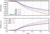Fig. 9 Time evolution of the simulated total energy (upper panel) and its relative deviation from its conserved value (lower panel) as obtained by the 2D Orszag-Tang test using GOEMHD3 in dependence on the mesh resolution of 1282 (red), 2562 (green), 5122 (blue), and 10242 (magenta) grid points. The black line overlaid in the upper panel corresponds to the volume energy density of 0.0697 rescaled from the surface density that was obtained by the ATHENA code run for 10242 grid points.

3.3. Resistive decay of a cylindrical current

GOEMHD3 was developed to simulate current carrying astrophysical plasmas taking into account current dissipation. This means that to describe solar flares, for example, magnetic reconnection has to be simulated, which needs resistivity. A locally increased resistivity is commonly assumed to do this, which is switched on after reaching a macroscopic current density threshold, for example. After this, the resistivity grows linearly or nonlinearly with the current density (see, e.g., Adamson et al. 2013). For this purpose, GOEMHD3 contains modules for spatial and also temporal smoothing of the resistivity, which keeps the simulations stable. To test the ability of GOEMHD3 to correctly describe the behavior of a resistive magneto-plasma, we tested it by applying different models of resistivity and comparing the simulation results with analytical predictions where possible. In particular, we applied a test setup simulating the resistive decay of a cylindrical current column in two spatial dimensions for which in certain limits analytical solutions exist (Skála & Bárta 2012).

Initially, at t = 0, a cylindrical current was set up using a radial magnetic field B = (0,B_φ,0), which is given by 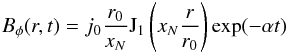$\begin{array}{ccc}{\mathit{B}}_{\mathit{\phi }}\mathrm{\left(}\mathit{r,t}\mathrm{\right)}\mathrm{=}{\mathit{j}}_{\mathrm{0}}\frac{{\mathit{r}}_{\mathrm{0}}}{{\mathit{x}}_{\mathit{N}}}{\mathrm{J}}_{\mathrm{1}}\left({\mathit{x}}_{\mathit{N}}\frac{\mathit{r}}{{\mathit{r}}_{\mathrm{0}}}\right)\exp \mathrm{(}\mathrm{-}\mathit{\alpha t}\mathrm{)}& & \end{array}$(21)in the internal (r ≤ r₀) region and by 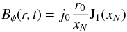$\begin{array}{ccc}{\mathit{B}}_{\mathit{\phi }}\mathrm{\left(}\mathit{r,t}\mathrm{\right)}\mathrm{=}{\mathit{j}}_{\mathrm{0}}\frac{{\mathit{r}}_{\mathrm{0}}}{{\mathit{x}}_{\mathit{N}}}{\mathrm{J}}_{\mathrm{1}}\mathrm{\left(}{\mathit{x}}_{\mathit{N}}\mathrm{\right)}& & \end{array}$(22)in outer space (r>r₀). Here j₀ = 1 is the amplitude of the current density on the axis of the cylinder, and r₀ = 1 is the radius of the current column, J_l(x) denotes a Bessel function of the order l, and x_N ≈ 2.40 is its first root J₀(x). The decrement (current decay rate) α is defined as α = η(x_N/r₀)². The pressure was chosen uniformly (p = 1) in the whole domain and the density was set to a very high uniform value (ρ = 10³²) that effectively sets the plasma at rest. Then the system of MHD Eqs. (1)–(4)) reduces to the induction Eq. (3), which in special cases can be solved analytically. For the GOEMHD3 test simulations the computational domain was chosen as [− 2.5,2.5] × [−2.5,2.5] and open boundary conditions were applied in the y and z directions. Periodic boundary conditions were used in the invariant (x-) direction.

We simulated the consequences of resistivity for the evolution of electrical currents by using GOEMHD3 considering the decay of a current column in response to two different resistivity models – a sharp step-function-like and a smooth change of the resistivity.

Step function model of resistivity.

In this model the resistivity was set η = 0.1 in the internal region, while in outer space it was set to zero. For this step function of the resistivity distribution, Skála & Bárta (2012) found an analytic solution of the induction equation describing the time-dependent evolution of the magnetic field and current in the cylinder. According to this solution, the current decays exponentially, and an infinitesimally thin current ring is induced around the resistive region according to $\begin{array}{ccc}{\mathit{j}}_{\mathit{x}}\mathrm{\left(}\mathit{r,t}\mathrm{\right)}& \mathrm{=}& {\mathit{j}}_{\mathrm{0}}{\mathit{J}}_{\mathrm{0}}\left({\mathit{x}}_{\mathit{N}}\frac{\mathit{r}}{{\mathit{r}}_{\mathrm{0}}}\right)\exp \mathrm{(}\mathrm{-}\mathit{\alpha t}\mathrm{)}\mathrm{+}\frac{{\mathit{j}}_{\mathrm{0}}}{\mathrm{2}\mathit{\pi }{\mathit{x}}_{\mathit{N}}}{\mathit{J}}_{\mathrm{1}}\mathrm{\left(}{\mathit{x}}_{\mathit{N}}\mathrm{\right)}\\ & & \mathrm{\times }\left[\mathrm{1}\mathrm{-}\exp \mathrm{(}\mathrm{-}\mathit{\alpha }{\mathit{t}}^{\mathrm{)}}\right]\mathit{\delta }\mathrm{(}\mathit{r}\mathrm{-}{\mathit{r}}_{\mathrm{o}}\mathrm{)}\mathit{,}\end{array}$(23)where δ(x) is the Dirac delta function. As a result of the discretization of the equations instead of a Dirac delta function shape, the current ring has a finite width, which, in our case, extends over two grid-points while the magnitude of the current inside this ring is finite.

Fig. 10 GOEMHD3 simulation of the time evolution of the current density jx at the center of a current cylinder assuming a step-function change of the resistivity. Colored lines correspond to different mesh resolutions employed for the simulations. The solid black line corresponds to the analytic solution given by Eq. (23).

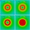Fig. 11 Magnetic field strength | B | in the y-z-plane at time t = 0.1τA for the step-function-like change of the resistivity changing with mesh resolution. Panels a)–d) correspond to a resolution of 1282, 2562, 5122, and 10242 grid points, respectively.

Figure 10 shows that, initially, the decay of the current density in the center closely follows the time evolution of the analytic solution (Eq. (23)), while a sharp drop to zero is observed at later times depending on the numerical resolution of the grid. Figure 10 shows that the drop of the current density at the center of the column is steeper and occurs earlier the better the grid resolution is. This is due to a numerical instability which spreads starting from the sharp edge of the resistive cylinder propagating toward its center. The growth rate and speed of propagation of this instability increases with the grid resolution, as illustrated in Fig. 11. The figure shows the magnetic field strength | B | in the y-z-plane at time t = 0.1τ_A for four different mesh resolutions corresponding to 128², 256², 512², and 1024² grid points. This dependence on resolution strongly indicates that the numerical origin of the instability is caused by the sharp resistivity in this model. To verify this hypothesis, we also tested another model in which the resistivity changes not by a step-function-like jump, but smoothly, as is typically encountered in astrophysical applications.

Smooth change of resistivity model.

Indeed, GOEMHD3 is meant to treat collisionless astrophysical plasmas, like that of the solar corona, by a fluid approach, while the resistivity (as other transport properties) is due to micro-turbulence, which is not described by the MHD equations. As a good compromise, smoothly changing resistivity models are often assumed to include this microphysics-based phenomenon in the fluid description. Smoothly changing switch-on models of resistivity are well suited to mimic the consequences of kinetic-scale processes. To test the influence of a resistivity changing smoothly in space and time, we used the same setup as described in the previous paragraph and only replaced the step-like jump function by a smooth resistivity change according to 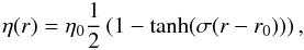$\begin{array}{ccc}\mathit{\eta }\mathrm{\left(}\mathit{r}\mathrm{\right)}\mathrm{=}{\mathit{\eta }}_{\mathrm{0}}\frac{\mathrm{1}}{\mathrm{2}}\left(\mathrm{1}\mathrm{-}\tanh \mathrm{\left(}\mathit{\sigma }\mathrm{\right(}\mathit{r}\mathrm{-}{\mathit{r}}_{\mathrm{0}}\mathrm{\left)}\mathrm{\right)}\right)\mathit{,}& & \end{array}$(24)where now η₀ = 0.1 and σ is a smoothness parameter. Figure 12 shows the results obtained for a smoothness parameter σ = 32. It indicates that a smooth resistivity change immediately solves the problem of oscillatory instabilities arising for a step-function-like resistivity change. As there is no analytical solution known for the smooth switch-on resistivity, we also show in Fig. 12 (by the black line) the result of the analytical prediction obtained for a step-function-like change of the resistivity. The simulated current decay is very similar to the analytically predicted decay for the step-function-like jump of the resistivity. The slight deviation of the curves from the predicted decay at later times might be due to the lower resistivity values that arise in the smooth model at the edge of the resistive cylinder (r → r₀) compared to those typical for the step-function model. We note that the steepness parameter σ = 32 in Eq. (24) allowed a stable simulation of the current decay already for the relatively coarse mesh resolution of 128² grid points, as shown in Fig. 12. We tested with additional test runs (not shown here) the stability of the simulations for even steeper resistivity changes and found that GOEMHD3 can easily cope with changes characterized by steepness parameters 64, 128, and higher, as long as the grid resolution is increased accordingly.

Finally, we conclude that by testing different models of changing resistivity, we were able to demonstrate that GOEMHD3 can simulate the consequences of localized resistive dissipation with sufficient accuracy, provided the changes are not step-function-like.

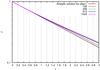Fig. 12 GOEMHD3 simulation of the time evolution of the current density jx at the center of a current cylinder assuming a smooth change of the resistivity. Colored lines correspond to different mesh resolutions employed for the simulations. Note that, since no analytical solution exists for this problem, the solid black line still corresponds to the analytic solution for a step-funtion-like change of the resistivity as given by Eq. (23) – as in Fig. 10.

3.4. Harris current sheet

To assess the effective numerical dissipation rate for the leap-frog scheme in the nonlinear regime, we simulated a Harris-like current sheet in the framework of an ideal plasma (see, e.g., Kliem et al. 2000). The size of the simulation box was set to [− 10.0,10.0] × [−0.6,0.6] with an open boundary in y-direction and periodic boundary conditions in z-direction. The initial conditions read 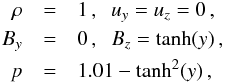$\begin{array}{ccc}\mathit{\rho }& \mathrm{=}& \mathrm{1}\hspace{0.17em}\mathit{,}{\mathit{u}}_{\mathit{y}}\mathrm{=}{\mathit{u}}_{\mathit{z}}\mathrm{=}\mathrm{0}\hspace{0.17em}\mathit{,}\\ {\mathit{B}}_{\mathit{y}}& \mathrm{=}& \mathrm{0}\hspace{0.17em}\mathit{,}{\mathit{B}}_{\mathit{z}}\mathrm{=}\tanh \mathrm{\left(}\mathit{y}\mathrm{\right)}\hspace{0.17em}\mathit{,}\\ \mathit{p}& \mathrm{=}& \mathrm{1.01}\mathrm{-}{\tanh }^{\mathrm{2}}\mathrm{\left(}\mathit{y}\mathrm{\right)}\hspace{0.17em}\mathit{,}\end{array}$(25)and the physical resistivity is η = 0.

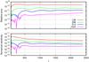Fig. 13 Time evolution of the relative deviation | ΔBz/ tanh(ym) | of the magnetic field from the analytical prediction (top) and derived effective numerical resistivity ηn (bottom) at position (ym,zm) = (−0.5493,0) for the simulation of a Harris-like current sheet. Results for different spatial resolutions (number of grid points in y direction) are color-coded according to the legend. The high-frequency oscillations are caused by the mesh drift instability of the staggered leap-frog scheme, which is not explicitly damped in this simulation setup (cf. Sect. 2.2).

We measured the time-variation of the magnetic field, B_z, at point (y_m,z_m) = (−0.5493,0) where the field attains half of its maximum magnitude. The effective numerical resistivity of the discretization scheme can then be estimated by $\begin{array}{ccc}{\mathit{\eta }}_{\mathit{n}}\mathrm{=}\frac{\mathrm{\Delta }{\mathit{B}}_{\mathit{z}}}{\mathrm{\Delta }\mathit{t}}\mathrm{·}{\left(\frac{{\mathit{\partial }}^{\mathrm{2}}{\mathit{B}}_{\mathit{z}}}{\mathit{\partial }{\mathit{y}}^{\mathrm{2}}}\right)}^{-1}\mathit{,}& & \end{array}$(26)where ΔB_z = B_z(y_m,z_m)−tanh(y_m) is the difference between the numerical and the analytical solution for the magnetic field, Δt represents the time of the measurement, and the second derivative of B_z is approximated by a standard finite-difference representation. Figure 13 shows the time evolution of the numerical dissipation rate, η_n, of the code for different values of the mesh resolution in y direction (a constant number of eight grid points was used in the invariant z direction). The relative numerical error of B_z and hence the estimate of the numerical resistivity settle at very low values, for instance, η_n ≃ 10^-14 and | ΔB_z/ tanh(y_m) | ≃ 5 × 10^-11 for the simulation with 256 × 8 grid points.

We conclude that the residual intrinsic numerical dissipation of the discretization scheme is negligible compared with the physical resistivities and explicit numerical stabilization measures that typically apply in simulations with GOEMHD3. We complement this idealized 1D test below by estimates for the effective numerical dissipation rate obtained in fully 3D simulations of an eruptive solar region (see Sect. 4.5).

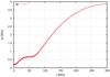Fig. 14 Grid spacing dz in the z-direction in the simulation of the AR 1429, where z = 0 is the photosphere. The finer spacing at the bottom part samples the transition region better with steep gradients in the density and temperature.

4. Three-dimensional simulations of the solar corona with GOEMHD3

To demonstrate the applicability of the GOEMHD3 code to realistic, 3D simulations of weakly collisional astrophysical plasmas at high Reynolds numbers and to assess the computational performance of the code, we simulated the evolution of the solar corona above an active region. Being able to simulate such scenarios, where a number of important dynamical processes are still not well understood, has in fact been the main motivation for developing GOEMHD3. As we show below, GOEMHD3 allows us to numerically tackle such problems with significantly higher numerical resolution and accuracy than was possible with its predecessor codes.

4.1. Physical context

We chose for this demonstration the solar corona above active region NOAA AR 1429 in March 2012. This active region is well known since it released many prominent phenomena, such as strong plasma heating, particle acceleration, and even eruptions. Many of them took place during the two weeks between March 2 and 15, 2012, making AR1429 one of the most active regions during solar cycle 24. They were observed in detail using the AIA instrument onboard of NASA’s Solar Dynamics Observatory SDO, for instance (see, e.g., Inoue et al. 2014; van Driel-Gesztelyi et al. 2014; Möstl et al. 2013). Very sensitive information was obtained about MeV energy (relativistic) electron acceleration processes, for example, which is provided by 30 THz radio waves. Examining the role of the continuum below the temperature minimum with a new imaging instrument operating at El Leoncito, Kaufmann et al. (2013) studied the 30 THz emissions. For the M8 class flare on March 13, 2012, for example, they found a very clear 30 THz signature, much cleaner than the white-light observations are able to provide. Another important information obtained about the solar activity are the dynamic spectra of solar proton emissions. The PAMELA experiment, for instance, measures the spectra of strongly accelerated protons over a wide energy range. For four eruptions of AR 1429 the observed energetic proton spectra were analyzed by Martucci et al. (2014). The authors interpreted the eruptions as an indication of first-order Fermi acceleration, that is, of a mirroring of the protons between dynamically evolving plasma clouds in the corona above AR 1429. Changes in the chemistry of the Earth’s atmosphere after the impact of the energetic solar protons emitted by AR 1429 were studied by von Clarmann et al. (2013). These authors used the MIPAS spectrometer onboard the now defunct European environmental satellite ENVISAT to measure temperature and trace gas profiles in the Earth’s atmosphere. They found that the amount of energetic solar protons produced by AR 1429 was among the 12 largest solar-particle events, also known as proton storms, in 50 years. These and more observations of AR 1429 indicate that very efficient energy conversion processes took place in the corona.

4.2. Initial and boundary conditions

We started the simulation with initial conditions derived in accordance with observations of AR 1429 on March 7, 2012, when at 00:02 UT a X5.4 flare eruption took place at heliographic coordinates N18E31. To describe the evolution of the corona before the eruption, we initialized the simulation using photospheric magnetic field observations obtained on March 6 at 23:35 UT. Figure 16 shows the line-of-sight (LOS) component of the photospheric magnetic field of AR 1429 obtained at this time by the HMI instrument onboard the SDO spacecraft in a field of view of 300 × 300 arcsec². This field of view covers an area of 217.5 × 217.5 Mm², which we chose as the lower boundary of the simulation box. The line-of-sight magnetic field was preprocessed by flux balancing, removing small-scale structures and fields close to the boundary before it was used for extrapolation into 3D. In particular, a spatial 2D Fourier filtering of the magnetic field data was applied to remove short spatial wavelength modes with wave numbers greater than 16, which correspond to structures that do not reach out into the corona, above the transition region. The Fourier-filtered magnetic fields were flux balanced and extrapolated into the third dimension according to the MHD box boundary conditions derived by Otto et al. (2007). The resulting initial magnetic field is depicted in Fig. 17. For the height of the simulation box we chose 300 Mm. The simulation grid spacing in the x and y directions is homogeneous with a mesh resolution given by the sampling over 258² grid points. After filtering out all modes with wave numbers larger than 16, this grid allows resolving all magnetic field structures sufficiently well. In the height (z-) direction we also used 258 grid points, but the grid was nonuniformly distributed to better resolve the lower part of the corona, that is, transition region and chromosphere. Figure 14 shows the height-dependent grid spacing (dz) used.

The initial density distribution was prescribed such that the chromospheric density is 500 times higher than the density in the corona according to the equation $\begin{array}{ccc}\mathit{\rho }\mathrm{\left(}\mathit{z}\mathrm{\right)}\mathrm{=}\frac{{\mathit{\rho }}_{\mathrm{ch}}}{\mathrm{2}}\left[\mathrm{1}\mathrm{-}\tan \mathrm{(}\mathrm{2}{\mathrm{(}\mathit{z}\mathrm{-}{\mathit{z}}_{\mathrm{0}}\mathrm{)}}^{\mathrm{)}}\right]\mathrm{+}{\mathit{\rho }}_{\mathrm{co}}\mathit{,}& & \end{array}$(27)where, ρ_ch and ρ_co are chromospheric and coronal densities. We note that the normalizing density was ρ₀ = 2 × 10¹⁵ m^-3. The transition region was initially localized around z₀ = 3, which corresponds to 15 Mm. The initial thermal pressure p = 0.01p₀ = 0.7957 Pa was homogeneous throughout the whole simulation domain, meaning that gravity effects were neglected. According to the ideal gas law T = p/ (k_BN), this reveals the temperature height profile. The initial density and temperature height profiles are depicted in Fig. 15. The initial coronal temperature is on the order of 10⁶ K. The initial plasma velocity is zero everywhere in the corona, but finite in the chromosphere.

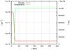Fig. 15 Initial height profiles of density and temperature in the simulation of AR 1429. The chromospheric density is 500 times higher than the density in the corona. The transition region is initially localized around z0 = 3, which corresponds to 15 Mm.

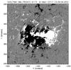Fig. 16 Magnetogram of active region 1429 on March 6, 2012, as taken by HMI onboard SDO.

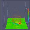Fig. 17 Initial structure of the magnetic field in the parallel scaling tests. The field is current-free and is extrapolated from the 2D magnetogram of AR1429 by the Fourier method. The evolution is triggered by a divergence-free velocity vortex located in the positive magnetic footpoint.

For the sides of the simulation box, the boundary conditions were set according to the MHD-equation-compatible line symmetry conditions derived by Otto et al. (2007). The top boundaries were open, that is, $\frac{\mathit{\partial }}{\mathit{\partial z}}\mathrm{=}\mathrm{0}$, except for the normal to the boundary component of the magnetic field, which was obtained to fulfill the source-freeness condition ∇·B = 0. The bottom boundary of the simulation box was open for entropy and magnetic fluxes.

The coronal plasma was driven via a coupling to the neutral gas below the transition region. The neutral gas was driven in accordance with the observed photospheric motion. First, the plasma flow velocities were inferred from photospheric magnetic field observations according to Santos et al. (2008b). To avoid emerging and submerging magnetic fluxes, the motion pattern was then modeled by divergence-free vortices given by $\begin{array}{ccc}{{u}}_{\mathrm{0}}\mathrm{=}\mathrm{\nabla }\mathrm{\times }\left[\frac{{\mathit{\phi }}_{\mathrm{0}}}{\cosh \mathrm{(}{\frac{\mathit{x}\mathrm{-}\mathit{y}\mathrm{+}{\mathit{c}}_{\mathrm{0}}}{{\mathit{l}}_{\mathrm{0}}}}^{\mathrm{)}}\cosh \mathrm{(}{\frac{\mathit{x}\mathrm{+}\mathit{y}\mathrm{+}{\mathit{d}}_{\mathrm{0}}}{{\mathit{l}}_{\mathrm{1}}}}^{\mathrm{)}}}\right]\hat{{z}}\mathit{.}& & \end{array}$(28)The parameters determining strength and localization of the vortex motion were chosen in accordance with observations. In the simulated case the magnetic fluxes rotate around footpoints given by the set of parameters φ₀ = 0.1, c₀ = 9, d₀ = −49, l₀ = 2, and l₁ = −2. The strength of the plasma driving by the neutral gas decreases with the height above the photosphere. This decrease is controlled by a height-dependent coupling term in the momentum equation Eq. (2) (or Eq. (9)). The height-dependent collision coefficient is defined as $\begin{array}{ccc}\mathit{\nu }\mathrm{\left(}\mathit{z}\mathrm{\right)}\mathrm{=}\frac{{\mathit{\nu }}_{\mathrm{0}}}{\mathrm{2}}\left[\mathrm{1}\mathrm{-}\tanh \mathrm{\left(}\mathrm{20}\mathrm{\right(}\mathit{z}\mathrm{-}{\mathit{z}}_{\mathrm{c}}\mathrm{\left)}\mathrm{\right)}\right]\mathit{.}& & \end{array}$(29)For the simulated case a good approximation for the coupling coefficient is ν₀ = 3 with and z_c = 0.25 (or 1.25 Mm) as the characteristic height, where the coupling (and, therefore, the photospherically caused plasma driving) vanishes.

4.3. Computational performance of GOEMHD3

Employing the physical setup (i.e., initial and boundary conditions) described in the previous subsection, the parallel scalability and efficiency of the GOEMHD3 code was assessed across a wide range of CPU-core counts and for different sizes of the numerical mesh. The benchmarks were performed on the high-performance-computing system of the Max Planck Society, Hydra, which is operated by its computing center, the RZG. Hydra is an IBM iDataPlex cluster based on Intel Xeon E5-2680v2 Ivy Bridge processors (two CPU sockets per node, ten cores per CPU socket, operated at 2.8 GHz) and an InfiniBand FDR 14 network. Hydra’s largest partition with a fully nonblocking interconnect comprises 36 000 cores (1800 nodes). For the benchmarks Intel’s FORTRAN compiler (version 13.1) and runtime were used together with the IBM parallel environment (version 1.3) on top of the Linux (SLES11) operating system.

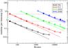Fig. 18 Computing time per time step (open circles) as a function of the number of CPU cores. Two MPI tasks, each spawning ten OpenMP threads that are assigned to the ten cores of a CPU socket were used on each of the two-socket nodes, i.e., the total number of MPI tasks is ten times smaller than the number of CPU cores given on the abscissa. Different colors correspond to different sizes of the numerical grid. Dashed inclined lines indicate ideal strong scalability for a given grid size. Two sets of measurements in which both the number of grid points and the number of processor cores was increased by a factor of 23 from left to right are marked by filled circles. The horizontal dotted lines are a reference for ideal weak scalability. The diamond symbols correspond to additional runs that employed a plain MPI parallelization (OpenMP switched off), i.e., the number of MPI tasks equals the number of cores.

Figure 18 provides an overview of the parallel performance of GOEMHD3, using the execution time for a single time step⁶ as a metric. Four different grid sizes were considered: grids with 256³ cells (black), 512³ cells (red), 1024³ cells (green), and 2048³ cells (blue). The figure demonstrates the very good overall strong scalability of the code, that is, the reduction of the computing time for fixed grid size with an increasing number of CPU cores (compare the measured runtimes plotted as circles with the dashed lines of the same color that indicate ideal scalability). For example, the parallel efficiency is at the 80% level for the 1024³ grid on 2580 cores (128 nodes) when compared to the baseline performance on 160 cores (8 nodes). Simulations with a 2048³ grid can be performed with a parallel efficiency of 80% on more than 10 000 cores.

Increasing the number of grid points by a factor of 8 (from 256³ to 512³, or from 512³ to 1024³) and at the same time using eight times as many CPU cores, the computing time remains almost constant (compare the two sets of filled circles with the corresponding horizontal dotted lines in Fig. 18). This demonstrates the very good weak scalability of GOEMHD3, given that the complexity of the algorithm scales linearly with the number of grid points.

The deviations from the ideal (strong) scaling curves that become apparent at high core counts are due to the relatively longer fraction of time spent in the MPI communication (halo exchange) between the domains. For example, for the 1024³ grid, the percentage of communication amounts to 30% for 10 000 cores and increases to about 50% at 36 000 cores. For a given number of cores, the communication-time share is longer for smaller grids (visible as a stronger deviation from ideal scalability in Fig. 18). The latter observation underlines the benefit of making the MPI domains as large as possible, which is enabled by our hybrid MPI-OpenMP parallelization approach (cf. Sect. 2.3). Moreover, by comparison with runs where the OpenMP parallelization was switched off and computer nodes were densely populated with MPI tasks (one MPI task per core), the advantages of the hybrid MPI-OpenMP vs. a plain MPI parallelization become immediately apparent. The smaller size of the MPI domains in the plain MPI runs (diamond symbols in Fig. 18) accounts for a higher communication-to-computation ratio and a larger number of smaller MPI messages. Accordingly, the communication times increase by about 75%, resulting in total runtimes being longer by 15–30% than the hybrid version using the same number of cores. It is crucial for the hybrid approach to achieve a close-to-perfect parallel efficiency of the OpenMP parallelization within the MPI domains so as not to jeopardize the performance advantages of the more efficient communication. Additional benchmarks have shown that GOEMHD3 indeed achieves OpenMP efficiencies close to 100% up to the maximum number of cores a single CPU socket provides (ten cores on our benchmark platform), but – as a result of the effects of NUMA⁷ and limited memory bandwidth – not beyond.

Overall, GOEMHD3 achieves a floating-point performance of about 1 GFlops/s per core, which is about 5% of the theoretical peak performance of the Intel Xeon E5-2680v2 CPU. Floating-point efficiencies in this range are commonly considered reasonable for this class of finite-difference schemes.

4.4. 3D simulation of the energy distribution in the photospherically driven solar corona

To understand the dependence of the energy distribution in the corona on the inflow of mechanical, thermal, and magnetic (Poynting flux) energy from below, through the transition region, we calculated the corresponding coronal energy contents and the fluxes through the transition region.

The energies were calculated based on their change rates as $\begin{array}{ccc}{\mathit{E}}_{\mathrm{kin}}& \mathrm{=}& \int [\mathrm{-}\frac{\mathrm{1}}{\mathrm{2}}{\mathrm{\int }}_{\mathit{S}}\mathit{\rho }{\mathit{u}}^{\mathrm{2}}{u}\mathrm{·}\mathrm{d}{S}\\ & & \mathrm{-}\frac{\mathrm{1}}{\mathrm{2}}{\mathrm{\int }}_{\mathit{V}}\left({u}\mathrm{·}{\nabla }\mathit{p}\mathrm{+}{u}\mathrm{·}{j}\mathrm{\times }{B}\right)\mathrm{d}\mathit{V}]\mathrm{d}\mathit{t}\\ {\mathit{E}}_{\mathrm{mag}}& \mathrm{=}& \int [{\mathrm{\int }}_{\mathit{S}}\mathrm{(}\mathrm{-}{u}{\mathit{B}}^{\mathrm{2}}\mathrm{+}\mathrm{(}{u}\mathrm{·}{{B}}^{\mathrm{)}}{B}\mathrm{-}\mathit{\eta }{j}\mathrm{\times }{{B}}^{\mathrm{)}}\mathrm{·}\mathrm{d}{S}\\ & & \mathrm{+}{\mathrm{\int }}_{\mathit{V}}\mathrm{(}\mathrm{-}{u}\mathrm{·}{j}\mathrm{\times }{B}\mathrm{-}\mathit{\eta }{\mathit{j}}^{\mathrm{2}}\mathrm{)}\mathrm{d}\mathit{V}]\mathrm{d}\mathit{t}\\ {\mathit{E}}_{\mathrm{th}}& \mathrm{=}& \int [\frac{\mathrm{-}\mathit{\gamma }}{\mathrm{2}\mathrm{(}\mathit{\gamma }\mathrm{-}\mathrm{1}\mathrm{)}}{\mathrm{\int }}_{\mathit{S}}\mathit{p}{u}\mathrm{·}\mathrm{d}{S}\\ & & \mathrm{+}\frac{\mathrm{1}}{\mathrm{2}}{\mathrm{\int }}_{\mathit{V}}\mathrm{(}{u}\mathrm{·}\mathrm{\nabla }\mathit{p}\mathrm{+}\mathit{\eta }{\mathit{j}}^{\mathrm{2}}\mathrm{)}\mathrm{d}\mathit{V}]\mathrm{d}\mathit{t}\mathit{.}\end{array}$We note that the main contributions to the surface integrals (${{\mathrm{\int }}^{}}_{\mathit{S}}$) are mainly due to energy fluxes through the transition region. The latter is taken as the lower boundary for the volume integrals (${{\mathrm{\int }}^{}}_{\mathit{V}}$). At the same time, the energy fluxes through the side boundaries cancel each other due to the symmetric boundary conditions, and the fluxes through the upper boundary are negligibly weak.

To investigate the dependence of the energy distribution on the dissipative properties of the coronal plasma, we started to impose the photospheric-chromospheric driving on a corona with commonly assumed large Reynolds numbers (weakly dissipative). The simulation was initiated with a very low background resistivity η = 10^-10. As a result of our normalization length, the corresponding characteristic Reynolds number based on the normalizing Alfvén speed, that is, the Lundquist number, is on the order of 10¹⁰; at the grid resolution scale it is still 2 × 10⁹. After t = 100τ_A (~1025 s), when enhanced activity was observed at the Sun, the background resistivity was enhanced to η = 10^-2, which corresponds to microturbulence theory predictions of Silin & Büchner (2003a) and Silin & Büchner (2003b). Figure 19 depicts the temporal evolution of the kinetic, magnetic, and thermal energies within the corona above the transition region and the energy fluxes into/from the corona across the transition region. Note that the curves in the figure correspond to the net changes of the energy, that is, the excess from the initial values at t = 0. The figure shows that the main energy source for the corona is the Poynting flux generated by the footpoint motion of the flux tubes, not the direct transfer of kinetic energy from the chromosphere. Until about t = 20τ_A (about 200 s, slightly more than 3 min), the magnetic energy inflow mainly enhances the kinetic energy of the corona, meanign that the coronal flux tubes are driven by the photospheric motion. This process lasts as long as the average propagation time of the corresponding Alfvenic perturbation along typical flux tubes. Hence this Alfven transition time is needed to drive, finally, the whole flux tube system. After this, the amount of magnetic energy in the corona steadily increases until, at t = 100τ_A, that is, after about 1000 s (i.e., about 17 min), the resistivity is increased by orders of magnitude (see above). Now the enhanced resistivity (the magnetic diffusivity) quickly heats the corona. After only 80τ_A (800 s or 13 min), the thermal energy enhancement of the corona due to the imposed Joule heating almost reaches the level of the kinetic energy enhancement due to the footpoint motion. At the same time, the increase of the magnetic energy contents of the corona due to the permanent Poynting flux inflow is slowed down only slightly by the heating process.

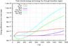Fig. 19 Scaling test simulating the solar corona above AR 1429. We show the temporal evolution of thermal, kinetic, and magnetic energies within corona above the transition region. The energy fluxes of the thermal, kinetic, and magnetic energies from the chromosphere are denoted by flux. For the meaning of the different lines see the line form legend. After t ~ 16 min the background resistivity is enhanced, causing Joule heating.

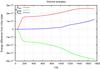Fig. 20 Scaling test simulation of the solar corona above AR 1429: temporal evolution of the thermal, kinetic, and magnetic volumetric energies in the solar atmosphere above the transition region. For the meaning of the different lines see the line form legend. Note that after the time t ~ 16 min the resistivity and, therefore, Joule heating, is essentially enhanced.

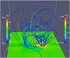Fig. 21 Snapshot of the magnetic field at the time t = 130τA (~22 min) of the simulated AR 1429. The magnetic field lines are colored according to the magnitude of the current carrier velocity j/n. The bottom plane depicts the magnetic field Bz component (perpendicular to the plane). A movie is available online.

To better understand the change of the coronal energy distribution, Fig. 20 depicts the temporal evolution of its kinetic, magnetic, and thermal energy contents without taking into account the contribution of energy inflows across the transition region. First, after the Alfvenic transition time has passed, in the course of the almost ideal (large Reynolds number) evolution, practically only the kinetic energy of the corona grows completely at the expense of the decreasing magnetic field energy. Then, after the magnetic diffusivity is enhanced at t = 100τ_A, the magnetic energy drops faster as a result of resistive dissipation. The latter enhances the thermal energy contents of the corona via Joule heating. After t = 170τ_A, the amount of the released energy within the corona is about half of the kinetic energy, as we showed in Fig. 19.

The time evolution of the magnetic field is captured by a movie that can be downloaded⁸.

The movie shows that until the moment when the resistivity, that is, the magnetic diffusivity is enhanced (after about 16 min solar time), the coronal magnetic fields evolves almost ideally, it is only bent following the footpoint motion, while the magnetic flux tubes are kept low. Only after the current carrier velocity (color-coded along the field lines) j/n becomes high enough, that is, after the micro-turbulence threshold is reached, the flux tubes start to rise faster. The reason for this is that the enhanced current dissipation allows magnetic diffusion and heating. After this, the magnetic flux tubes continue to rise even faster, releasing parts of the high magnetic tension until, finally, reconnection starts, the most efficient magnetic energy release process. Figure 21 shows the magnetic field configuration reached at t = 130τ_A, that is, after about 22 min. The color-coding of the magnetic field lines depicts the actual values of V_CC = j/n. At the places where V_CC is enhanced above the threshold, the plasma is quickly heated by Joule current dissipation.

4.5. Estimate of the numerical dissipation

Using a simulation setup for an eruptive solar region similar to the one described in Sect. 4.2, we estimated the effective numerical dissipation rate for the leap-frog scheme in realistic 3D simulations with complete input physics (see also Sect. 3.4). The mesh resolution was set to 258³ grid points. The initial magnetic field was taken from the active region 11226 on June 7 2011, 06:16 UT. During a total simulation time of t = 2400 and about 9.66 × 10⁵ time steps, the field line apex rose from an initial altitude of z₀ = 3.2 to the final height, z_e = 29.0. As a result of the very low physical resistivity, the field line is frozen in to the plasma and the position of the second footpoint can be predicted by tracking photospheric plasma motions. In our simulation the displacement of the second footpoint from the predicted position was Δr_e = 0.02942, from which we can estimate the effective numerical resistivity at the end of the simulation: 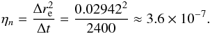$\begin{array}{ccc}{\mathit{\eta }}_{\mathit{n}}\mathrm{=}\frac{\mathrm{\Delta }{\mathit{r}}_{\mathrm{e}}^{\mathrm{2}}}{\mathrm{\Delta }\mathit{t}}\mathrm{=}\frac{{\mathrm{0.02942}}^{\mathrm{2}}}{\mathrm{2400}}\mathrm{\approx }\mathrm{3.6}\mathrm{\times }{\mathrm{10}}^{-7}\mathit{.}& & \end{array}$(33)The corresponding value of η_n for the times t = 20 and t = 240 are 1.47 × 10^-8 and 1.14 × 10^-7, respectively. Different values for η_n are obtained for different times because the computation of the footpoint displacement includes errors from the field line integration (which is very long at the end of the simulation) and also the from tracing the second footpoint over time. In summary, both the idealized 1D Harris current sheet (Sect. 3.4) and the application of GOEMHD3 to the full solar corona physics in three dimensions reveal no significant reconnection that would be due to numerical dissipation.

5. Discussion and conclusions

We have implemented a new 3D MHD code based on second-order-accurate finite-difference discretization schemes to be able to efficiently simulate large-scale weakly dissipative astrophysical plasma systems (systems with large Reynold number). To reduce numerical dissipation, the conservative part and source terms of the equations were solved by a leap-frog scheme that is second-order accurate in time and space. Only terms with second-order spatial derivatives, that is, viscosity, diffusion, and resistive dissipation, were discretized with a DuFort-Frankel scheme. Numerically induced grid-scale oscillations were damped away by introducing an artificial diffusivity that was switched on locally. We documented the main physical, numerical, and computational concepts of the new code GOEMHD3 and its computational performance. The code was tested and verified by means of a number of appropriate test problems that allowed us to reveal the limits of the applicability of GOEMHD3 and to describe the ways for achieving the goals when solving concrete problems.

The code was first tested by simulating a velocity-shear Kelvin-Helmholtz instability. Owing to the use of a low numerical dissipation leap-frog scheme, GOEMHD3 obtained the same linear evolution as simulations with the numerically more expensive, higher order PENCIL code. As expected, at later times, during the nonlinear evolution of the instability for the same number of grid points, the dissipation is higher than that of the higher order PENCIL code (McNally et al. 2012). The reason is artificial diffusivity, which is locally switched on to damp spurious grid-scale oscillations inherent to the leap-frog scheme. The amount of necessary damping can be easily and computationally cheaply reduced, however, by enhancing the grid resolution of the overall less expensive second-order scheme. We showed that GOEMHD3 solutions converge toward the solution obtained with PENCIL, and the resulting uncertainty (GCI, Fig. 5) agrees with the relative error (Fig. 4) of the GOEMHD3 (compared to PENCIL) mode amplitude evolution. GOEMHD3 revealed the same results for vortices of Orszag & Tang (1979) as obtained by Ryu et al. (1995) and by Dai & Woodward (1998). Gradients were well resolved by two grid-points. Numerical oscillations were smoothed by locally switching on diffusivity. GOEMHD3 dissipates more energy at steep wave fronts than a higher order code for the same grid-resolution. This dissipation can be easily overcome by (locally) using a larger number of grid points. The solver for the resistive part of the induction equation was tested separately by imposing a homogeneous resistivity on a current column. The results agree well with an analytically predicted current decay. The code fully reproduces the analytic solution until the enhanced numerical errors reach the center of the current system, where the current concentration is highest. Since the spreading of the numerical error only depends on the number of time steps, not on the real physical time, this phenomenon is of purely numerical nature. To cope with this effect, GOEMHD3 contains a module that smoothes an eventually self-regulated resistivity increase around the maximum gradient of the current growth. We showed that this resistivity smoothing is sufficient to keep simulations stable. In simulations of a 1D Harris current sheet and of a realistic 3D scenario with complete input physics, the residual numerical dissipation of GOEMHD3 was demonstrated to be sufficiently low to allow applications with almost ideal magneto-fluids at very high Reynolds number (Re ~ 10¹⁰). The parallel computing performance of the code was demonstrated by obtaining the scaling of the runtime with the number of CPU cores and grid points (i.e., different numerical resolutions) for a realistic application scenario. To this end, GOEMHD3 was initialized to simulate the evolution of the solar atmosphere above an observed active region and thus to obtain the distribution of the energy injected from the photosphere through the transition region into the corona. The calculations revealed an almost linearstrong scaling of the runtime with the number of CPU cores for meshes with up to 2048³ grid points. On the HPC system Hydra of the Max Planck Society, GOEMHD3 exhibited an almost ideal scaling even beyond 30 000 processor cores. In addition, we also obtained a very good weak scalability from 20 cores (1 node) for 256³ grid runs to more than 20 000 cores (1000 nodes) for a 2048³ grid, thereby maintaining absolute run times of shorter than a second per time step.

In summary, we showed that the new code GOEMHD3 is able to efficiently and accurately solve the MHD equations of almost ideal plasma systems on non-equidistant grids. As a result of its second-order-accurate discretization scheme, the code is conceptually straightforward to implement and to parallelize on distributed-memory computer architectures. The code can simply be adjusted to different types of initial and boundary conditions and extended to include additional physics modules. Its excellent computational performance and parallel efficiency enable compensating for the formally comparably low numerical accuracy per grid point and time step by adopting an enhanced resolution in space and time. Aiming at the same accuracy for the same problem, this is computationally still cheaper than running codes using higher order schemes.

Online material

Movie of Fig. 21 Access here

Acknowledgments

We gratefully acknowledge support of this work by the German Science Foundation Deutsche Forschungsgemeinschaft, DFG Collaborative Research Center 963, Project A02, by the Czech GACR project 13-24782S and the EU FP7-PEOPLE-2011-CIG programme PCIG-GA-2011-304265 (SERaF) as well as by Bernhard Bandow at the Max Planck Institute for Solar System Research. The authors thank Colin P. McNally, who provided data for the cross-code comparison, and the anonymous referee for valuable comments that helped to improve the quality of the paper.

References

All Figures

	Fig. 1 Color-coded mass density, ρ(y,z) at time t = 2.5 for the Kelvin-Helmholtz test problem. Panels a)–d) show the GOEMHD3 results for a numerical resolution of 1282, 2562, 5122, and 10242, respectively.
In the text

	Fig. 2 Time evolution of the y-velocity mode amplitude Ay (top panel) and of its growth rate Ȧy (bottom panel) in the course of the Kelvin-Helmholtz test. The results obtained by GOEMHD3 for different spatial resolutions are color-coded according to the legend. The black line corresponds to the result obtained by a PENCIL code run using a grid resolution of 40962 (McNally et al. 2012).
In the text

Fig. 3 Time evolution of the highest kinetic energy density ${\mathit{E}}_{\mathit{y}}\mathrm{=}\frac{\mathrm{1}}{\mathrm{2}}{\max }_{\mathit{y,z}}\mathrm{\left(}\mathit{\rho }{\mathit{u}}_{\mathit{y}}^{\mathrm{2}}\mathrm{\right)}$ in the Kelvin-Helmholtz test. The results obtained by GOEMHD3 for different spatial resolutions are color-coded according to the legend. The black line corresponds to the result of a PENCIL code run using a grid resolution of 40962 (McNally et al. 2012).

In the text

	Fig. 4 Time evolution of the relative error | εA | of the mode amplitude obtained for the Kelvin-Helmholtz test using GOEMHD3 compared to those obtained by the PENCIL code (McNally et al. 2012) for different numbers of grid points (color coded).
In the text

	Fig. 5 Time evolution of the grid convergence rate (top panel) of the mode amplitude in dependence on the spatial resolution given in the legend and of the grid convergence index GCI (bottom panel) of the mode amplitude uncertainty for the highest resolution.
In the text

	Fig. 6 Mass density distribution obtained at t = 0.25 for the 2D Orszag-Tang test. Panels a)–d) correspond to a mesh resolution of 1282, 2562, 5122, and 10242 grid points, respectively.
In the text

	Fig. 7 Thermal plasma pressure (panels a), e)), magnetic pressure (panels b), f)), vorticity ∇ × u (panels c), g)) and current density ∇ × B (panels d), h)) obtained for the 2D Orszag-Tang test by GOEMHD3 (top row) and ATHENA 4.2 (bottom row) for a grid resolution of 2562. t = 0.5.
In the text

	Fig. 8 Spatial distribution of the relative difference | ερ | of the mass density obtained by GOEMHD3 simulating the Orszag-Tang vortex problem comparing the results for three different mesh resolutions of a) 1282–2562; b) 2562–5122; and c) 5122–10242 grid points.
In the text

Fig. 9 Time evolution of the simulated total energy (upper panel) and its relative deviation from its conserved value (lower panel) as obtained by the 2D Orszag-Tang test using GOEMHD3 in dependence on the mesh resolution of 1282 (red), 2562 (green), 5122 (blue), and 10242 (magenta) grid points. The black line overlaid in the upper panel corresponds to the volume energy density of 0.0697 rescaled from the surface density that was obtained by the ATHENA code run for 10242 grid points.

In the text

	Fig. 10 GOEMHD3 simulation of the time evolution of the current density jx at the center of a current cylinder assuming a step-function change of the resistivity. Colored lines correspond to different mesh resolutions employed for the simulations. The solid black line corresponds to the analytic solution given by Eq. (23).
In the text

	Fig. 11 Magnetic field strength | B | in the y-z-plane at time t = 0.1τA for the step-function-like change of the resistivity changing with mesh resolution. Panels a)–d) correspond to a resolution of 1282, 2562, 5122, and 10242 grid points, respectively.
In the text

Fig. 12 GOEMHD3 simulation of the time evolution of the current density jx at the center of a current cylinder assuming a smooth change of the resistivity. Colored lines correspond to different mesh resolutions employed for the simulations. Note that, since no analytical solution exists for this problem, the solid black line still corresponds to the analytic solution for a step-funtion-like change of the resistivity as given by Eq. (23) – as in Fig. 10.

In the text

Fig. 13 Time evolution of the relative deviation | ΔBz/ tanh(ym) | of the magnetic field from the analytical prediction (top) and derived effective numerical resistivity ηn (bottom) at position (ym,zm) = (−0.5493,0) for the simulation of a Harris-like current sheet. Results for different spatial resolutions (number of grid points in y direction) are color-coded according to the legend. The high-frequency oscillations are caused by the mesh drift instability of the staggered leap-frog scheme, which is not explicitly damped in this simulation setup (cf. Sect. 2.2).

In the text

	Fig. 14 Grid spacing dz in the z-direction in the simulation of the AR 1429, where z = 0 is the photosphere. The finer spacing at the bottom part samples the transition region better with steep gradients in the density and temperature.
In the text

	Fig. 15 Initial height profiles of density and temperature in the simulation of AR 1429. The chromospheric density is 500 times higher than the density in the corona. The transition region is initially localized around z0 = 3, which corresponds to 15 Mm.
In the text

	Fig. 16 Magnetogram of active region 1429 on March 6, 2012, as taken by HMI onboard SDO.
In the text

	Fig. 17 Initial structure of the magnetic field in the parallel scaling tests. The field is current-free and is extrapolated from the 2D magnetogram of AR1429 by the Fourier method. The evolution is triggered by a divergence-free velocity vortex located in the positive magnetic footpoint.
In the text

Fig. 18 Computing time per time step (open circles) as a function of the number of CPU cores. Two MPI tasks, each spawning ten OpenMP threads that are assigned to the ten cores of a CPU socket were used on each of the two-socket nodes, i.e., the total number of MPI tasks is ten times smaller than the number of CPU cores given on the abscissa. Different colors correspond to different sizes of the numerical grid. Dashed inclined lines indicate ideal strong scalability for a given grid size. Two sets of measurements in which both the number of grid points and the number of processor cores was increased by a factor of 23 from left to right are marked by filled circles. The horizontal dotted lines are a reference for ideal weak scalability. The diamond symbols correspond to additional runs that employed a plain MPI parallelization (OpenMP switched off), i.e., the number of MPI tasks equals the number of cores.

In the text

Fig. 19 Scaling test simulating the solar corona above AR 1429. We show the temporal evolution of thermal, kinetic, and magnetic energies within corona above the transition region. The energy fluxes of the thermal, kinetic, and magnetic energies from the chromosphere are denoted by flux. For the meaning of the different lines see the line form legend. After t ~ 16 min the background resistivity is enhanced, causing Joule heating.

In the text

	Fig. 20 Scaling test simulation of the solar corona above AR 1429: temporal evolution of the thermal, kinetic, and magnetic volumetric energies in the solar atmosphere above the transition region. For the meaning of the different lines see the line form legend. Note that after the time t ~ 16 min the resistivity and, therefore, Joule heating, is essentially enhanced.
In the text

	Fig. 21 Snapshot of the magnetic field at the time t = 130τA (~22 min) of the simulated AR 1429. The magnetic field lines are colored according to the magnitude of the current carrier velocity j/n. The bottom plane depicts the magnetic field Bz component (perpendicular to the plane). A movie is available online.
In the text

References

- Adamson, E., Büchner, J., & Otto, A. 2013, A&A, 557, A118 [NASA ADS] [CrossRef] [EDP Sciences] [Google Scholar]
- Birn, J., & Priest, E. R. 2007, Reconnection of Magnetic Fields (Cambridge University Press) [Google Scholar]
- Büchner, J. 2007a, Plasma Physics and Controlled Fusion, 49, 325 [NASA ADS] [CrossRef] [Google Scholar]
- Büchner, J. 2007b, in New Solar Physics with Solar-B Mission, eds. K. Shibata, S. Nagata, & T. Sakurai, ASP, 369, 407 [Google Scholar]
- Büchner, J., & Nikutowski, B. 2005a, in Solar Wind 11/SOHO 16, Connecting Sun and Heliosphere, eds. B. Fleck, T. H. Zurbuchen, & H. Lacoste, ESA Sp. Publ., 592, 141 [Google Scholar]
- Büchner, J., & Nikutowski, B. 2005b, in Chromospheric and Coronal Magnetic Fields, eds. D. E. Innes, A. Lagg, & S. A. Solanki, ESA Sp. Publ., 596 [Google Scholar]
- Büchner, J., Dum, C., & Scholer, M. 2003, Space Plasma Simulation (Berlin: Springer Verlag), Lect. Notes Phys., 615 [Google Scholar]
- Büchner, J., Nikutowski, B., & Otto, A. 2004a, in SOHO 15 Coronal Heating, eds. R. W. Walsh, J. Ireland, D. Danesy, & B. Fleck, ESA Sp Publ., 575, 23 [Google Scholar]
- Büchner, J., Nikutowski, B., & Otto, A. 2004b, in Multi-Wavelength Investigations of Solar Activity, eds. A. V. Stepanov, E. E. Benevolenskaya, & A. G. Kosovichev, IAU Symp., 223, 353 [Google Scholar]
- Colella, P. 1990, J. Comput. Phys., 87, 171 [NASA ADS] [CrossRef] [Google Scholar]
- Colella, P., & Woodward, P. R. 1984, J. Comp. Phys., 54, 174 [Google Scholar]
- Dai, W., & Woodward, P. R. 1998, ApJ, 494, 317 [NASA ADS] [CrossRef] [Google Scholar]
- Elkina, N. V., & Büchner, J. 2006, J. Comp. Phys., 213, 862 [NASA ADS] [CrossRef] [Google Scholar]
- Evans, C. R., & Hawley, J. F. 1988, ApJ, 332, 659 [Google Scholar]
- Gudiksen, B. V., Carlsson, M., Hansteen, V. H., et al. 2011, A&A, 531, A154 [NASA ADS] [CrossRef] [EDP Sciences] [Google Scholar]
- Inoue, S., Hayashi, K., Magara, T., Choe, G. S., & Park, Y. D. 2014, ApJ, 788, 182 [NASA ADS] [CrossRef] [Google Scholar]
- Javadi, S., Büchner, J., Otto, A., & Santos, J. C. 2011, A&A, 529, A114 [NASA ADS] [CrossRef] [EDP Sciences] [Google Scholar]
- Kaufmann, P., White, S. M., Freeland, S. L., et al. 2013, ApJ, 768, 134 [NASA ADS] [CrossRef] [Google Scholar]
- Kliem, B., Karlický, M., & Benz, A. O. 2000, A&A, 360, 715 [NASA ADS] [Google Scholar]
- Martucci, M., Boezio, M., Bravar, U., et al. 2014, Nucl. Instrum. Methods Phys. Res. A, 742, 158 [NASA ADS] [CrossRef] [Google Scholar]
- McNally, C. P., Lyra, W., & Passy, J.-C. 2012, ApJS, 201, 18 [NASA ADS] [CrossRef] [Google Scholar]
- Möstl, U. V., Temmer, M., & Veronig, A. M. 2013, ApJ, 766, L12 [NASA ADS] [CrossRef] [Google Scholar]
- Orszag, S., & Tang, C. 1979, J. Fluid Mech., 90, 129 [NASA ADS] [CrossRef] [Google Scholar]
- Otto, A., Büchner, J., & Nikutowski, B. 2007, A&A, 468, 313 [NASA ADS] [CrossRef] [EDP Sciences] [Google Scholar]
- Press, W. H., Teukolsky, S. A., Vetterling, W. T., & Flannery, B. P. 2007, Numerical Recipes (Cambridge: Cambridge University Press) [Google Scholar]
- Roache, P. J. 1998, Verification and Validation in Computational Science and Engineering (Albuquerque: Hermosa publishers) [Google Scholar]
- Robertson, B. E., Kravtsov, A. V., Gnedin, N. Y., Abel, T., & Rudd, D. H. 2010, MNRAS, 401, 2463 [NASA ADS] [CrossRef] [Google Scholar]
- Ryu, D., Jones, T. W., & Frank, A. 1995, ApJ, 452, 785 [NASA ADS] [CrossRef] [Google Scholar]
- Santos, J. C., Büchner, J., Madjarska, M. S., & Alves, M. V. 2008a, A&A, 490, 345 [NASA ADS] [CrossRef] [EDP Sciences] [Google Scholar]
- Santos, J. C., Büchner, J., & Zhang, H. 2008b, Adv. Space Res., 42, 812 [NASA ADS] [CrossRef] [Google Scholar]
- Santos, J. C., Büchner, J., & Otto, A. 2011a, A&A, 535, A111 [NASA ADS] [CrossRef] [EDP Sciences] [Google Scholar]
- Santos, J. C., Büchner, J., & Otto, A. 2011b, A&A, 525, A3 [NASA ADS] [CrossRef] [EDP Sciences] [Google Scholar]
- Silin, I., & Büchner, J. 2003a, Phys. Plasmas, 10, 1299 [NASA ADS] [CrossRef] [Google Scholar]
- Silin, I., & Büchner, J. 2003b, Phys. Plasmas, 10, 3561 [NASA ADS] [CrossRef] [Google Scholar]
- Skála, J., & Bárta. 2012, Appl. Math., 3, 1842 [CrossRef] [Google Scholar]
- Springel, V. 2010, ARA&A, 48, 391 [NASA ADS] [CrossRef] [Google Scholar]
- Stone, J. M., & Gardiner, T. 2009, New A, 14, 139 [Google Scholar]
- Stone, J. M., Gardiner, T. A., Teuben, P., Hawley, J. F., & Simon, J. B. 2008, ApJS, 178, 137 [NASA ADS] [CrossRef] [Google Scholar]
- van Driel-Gesztelyi, L., Baker, D., Török, T., et al. 2014, ApJ, 788, 85 [NASA ADS] [CrossRef] [Google Scholar]
- von Clarmann, T., Funke, B., López-Puertas, M., et al. 2013, Geophys. Res. Lett., 40, 2339 [NASA ADS] [CrossRef] [Google Scholar]
- Wu, C.-C. 2007, Geophys. Astrophys. Fluid Dyn., 101, 37 [NASA ADS] [CrossRef] [Google Scholar]
- Yang, S., Büchner, J., Santos, J. C., & Zhang, H. 2013, Sol. Phys., 283, 369 [NASA ADS] [CrossRef] [Google Scholar]
- Yee, K.-S. 1966, IEEE Trans. Antennas Propag., 14, 302 [Google Scholar]