© ESO, 2015

1. Introduction

Hierarchical models of structure formation predict that galaxies form in small dark matter haloes that subsequently clump together and merge into larger ones (White & Rees 1978). At large scales, the evolution of structure is mainly determined by the properties of dark matter and dark energy. However, at smaller, galactic scales, baryonic physics cannot be ignored. Processes such as supernova and AGN feedback affect the relation between the observable (baryonic) properties of galaxies and their dark matter haloes. By measuring these relations, we hence gain insight into the processes that affected them. Studying this with numerical simulations is notoriously difficult, although in recent years this field has rapidly advanced through the use of semi-analytic models (e.g. Baugh 2006) and hydrodynamical simulations (e.g. Vogelsberger et al. 2014; Schaye et al. 2015). To test these simulations and guide them with further input, we need observations of the relation between the properties of galaxies and their dark matter haloes. This is also crucial for understanding the effect of baryonic physics on the dark matter power spectrum (e.g. van Daalen et al. 2011; Semboloni et al. 2011), which is the main observable in weak-lensing studies that aim to extract cosmological parameters, such as Euclid (Laureijs et al. 2011).

The properties of dark matter haloes around galaxies can be studied with weak gravitational lensing. As the photons emitted by distant galaxies traverse the Universe, they are deflected by the curvature of space around intervening mass inhomogeneities in the foreground. Consequently, the observed shapes of these background galaxies slightly deform, a distortion that can be reliably measured out to projected separations of tens of Mpcs around the lenses (e.g. Mandelbaum et al. 2013). Since this completely covers the regime where the dark matter halo of any lens dominates, weak gravitational lensing offers an excellent tool for measuring halo masses. The weak-lensing signal of individual galaxies is too noisy to be detected, but by averaging the signal of many lenses of similar observable properties, for instance in a certain luminosity range, we can learn about the average halo properties of such lens samples.

The relation between the properties of galaxies and their dark matter haloes has been studied before with weak lensing (e.g. Hoekstra et al. 2005; Mandelbaum et al. 2006b; Li et al. 2009; van Uitert et al. 2011; Brimioulle et al. 2013; Velander et al. 2014), but most of these studies focused on lenses at a limited redshift range. However, to study how galaxies evolve, one would like to measure how the luminosity-to-halo mass relation depends on lookback time. Recent imaging surveys such as the Canada-France-Hawaii Telescope Survey (CFHTLS) and the second Red-sequence Cluster Survey (RCS2) contain sufficient statistical power to enable such studies. Redshift-dependent constraints that are derived in a homogeneous way, as is done in this study, are particularly useful for numerical simulations, as they can potentially distinguish degeneracies among the model parameters and limit the space for fine-tuning to match low-redshift observations (for an example, see Fig. 23 in Guo et al. 2011).

In this work, we study a particular type of galaxies: luminous red galaxies (LRGs). They form an interesting subsample of the total population of galaxies, as they trace the highest density peaks in the Universe. These galaxies are thought to have formed around z ~ 2 during a relatively short and intense period of star formation, after which the formation of stars practically halted. Their luminosity evolution can therefore be approximately described by “passive evolution”, the evolution of a stellar population without forming new stars (e.g. Glazebrook et al. 2004; Cimatti et al. 2006; Roseboom et al. 2006; Cool et al. 2008; Banerji et al. 2010). This enables us to model the luminosity evolution, for example with stellar population synthesis models (e.g. Bruzual & Charlot 2003; Conroy et al. 2009, 2010; Maraston et al. 2009), and separate that from the halo mass evolution part. Low-level star formation and mergers may also contribute to the luminosity evolution of LRGs, but this is thought to mainly affect less massive LRGs (Scarlata et al. 2007; Pozzetti et al. 2010; Tojeiro & Percival 2010, 2011; Tojeiro et al. 2011, 2012). How strong the average effect is on the luminosity evolution compared to the pure passive evolution scenario is unclear. However, for massive and luminous LRGs, the luminosity evolution is thought to be well understood.

LRGs are advantageous to study also from an observational perspective. They are easily selected in multi-band optical datasets, and their redshifts can be relatively easily determined using the 4000 Å break (Eisenstein et al. 2001). More than a million LRGs have been observed spectroscopically as part of the Baryon Oscillation Spectroscopic Survey (BOSS; Dawson et al. 2013), forming the LOWZ sample, which targets z ≲ 0.4 galaxies, and the CMASS sample, which targets 0.4 <z< 0.7 galaxies. From a weak-lensing perspective, the advantage of LRGs is that they are massive and therefore produce a strong lensing signal that can be measured up to relatively high redshift. The overlap between the BOSS survey and the RCS2 therefore offers a perfect combined dataset on which to study the evolution of the luminosity-to-halo mass relation of LRGs.

The outline of this work is as follows. In Sect. 2 we describe the data that we use in this work, how we compute the luminosities, and how we perform the lensing analysis. We interpret the lensing measurements with the halo model, which we describe in Sect. 3. The evolution of the luminosity-to-halo mass relation is presented and discussed in Sect. 4. The mass-concentration relation is discussed in Sect. 5. We conclude in Sect. 6. Unless stated otherwise, we assume a WMAP7 cosmology (Komatsu et al. 2011) with σ₈ = 0.8, Ω_Λ = 0.73, Ω_M = 0.27, Ω_b = 0.046, and h₇₀ = H₀/ 70 km s^-1 Mpc^-1, with H₀ the Hubble constant; all distances are quoted in physical (rather than comoving) units; and all apparent magnitudes have been corrected using the dust maps from Schlegel et al. (1998).

2. Data analysis

We used data from the tenth data release (DR10; Ahn et al. 2014) from the Sloan Digital Sky Survey (SDSS; York et al. 2000) and from the second Red-sequence Cluster Survey (RCS2; Gilbank et al. 2011). As in van Uitert et al. (2011, 2013), Cacciato et al. (2014), we used the greater number of ancillary data on galaxies that is available from the SDSS compared with the RCS2 because the SDSS features photometry in five optical bands and includes spectroscopy for over a million of galaxies. However, the RCS2 imaging is ~2 mag deeper and achieved a median seeing of approximately 0.7′′, compared to 1.2′′ for SDSS, therefore the RCS2 is better suited for a weak-lensing analysis of lenses at higher redshifts. The total overlap between the RCS2 and the DR10 is about 450 square degrees.

A first combined analysis of the overlap between the ninth data release of SDSS (DR9; Ahn et al. 2012) and the RCS2 was presented in Cacciato et al. (2014), where the lensing signal of the DR9 galaxies with spectroscopy was studied using RCS2 galaxies as sources. In that work we did not study the redshift evolution of the lensing signal, because, in contrast to the current work, we studied a mixed sample of early- and late-type galaxies whose combined luminosity evolution was only poorly understood. In DR9, the number of (high-redshift) BOSS spectra was also only about half of that in DR10.

2.1. Lens sample

We used a subset of the total sample of overlapping DR10 galaxies with spectroscopy as our lenses, that is, only the LRGs. We selected all galaxies that have been targeted as part of BOSS. These are selected from the SDSS catalogues by requiring¹

• BOSS_TARGET1 && 2⁰

• SPECPRIMARY == 1

• ZWARNING_NOQSO == 0

• TILEID >= 10324

for the LOWZ sample, and

• BOSS_TARGET1 && 2¹

• SPECPRIMARY == 1

• ZWARNING_NOQSO == 0

• (CHUNK != “boss1”) && (CHUNK != “boss2”)

• i_fib2< 21.5

for the CMASS (high-z) sample. Additionally, we selected all objects with reliable spectroscopy from the SDSS catalogues that satisfy the BOSS LOWZ target selection cuts:

• | (r − i) − (g − r)/4−0.18 | < 0.2

• r< 13.5 + [ 0.7 × (g − r) + 1.2 × ((r − i) −0.18) ] /3

• $\mathrm{16}\mathit{<}\begin{array}{c}{}^{\mathrm{􏽥}}\\ \mathit{r}\end{array}\mathit{<}\mathrm{19.6}$

• SCIENCEPRIMARY==1

• ZWARNING_NOQSO == 0

• z_spec> 0.01

where g, r and i indicate model magnitudes and $\begin{array}{c}{\mathrm{􏽥}}^{}\\ \mathit{r}\end{array}$ cmodel magnitudes. Note that we replaced the BOSS selection criterion r_psf − r_cmod> 0.3 with z_spec> 0.01 to ensure that we have no stars. Finally, we also selected all objects that satisfied the CMASS selection cuts, but we found that all objects were already targeted and labelled as being BOSS galaxies, and it therefore did not increase the lens sample.

Even though the LOWZ and CMASS samples mainly consist of LRGs, the populations differ because of the different colour and magnitude selection cuts. Tojeiro et al. (2012) studied which fraction of the CMASS LRGs are progenitors of the LOWZ sample and found that this strongly depends on absolute magnitude, with the highest fractions found for the most luminous objects. A second but weaker trend is found with rest-frame colour. Therefore, we chose to analyse the LOWZ and the CMASS samples separately. We investigated, however, what we can conclude about the evolution of the luminosity-to-halo mass relation of LRGs if we consider the CMASS sample as progenitors of the LOWZ LRGs.

2.1.1. Luminosities

To study how the average halo mass of LRGs evolves, we compared LRGs at low redshifts to their predecessors at higher redshifts. To do this, we needed to obtain the luminosities of our LRGs, corrected for the redshift of their spectra through the passbands (i.e. the k-correction). We computed the k-correction using the code KCORRECT v4_2 (Blanton et al. 2003; Blanton & Roweis 2007), where we used the u, g, r, i and z model magnitudes and the spectroscopic redshift as input. Furthermore, we corrected for the intrinsic evolution of the luminosities (the e-correction), accounting for the difference between the observer-frame absolute magnitude of a galaxy with and without an evolving spectrum.

The luminosities of LRGs are thought to evolve passively, which can be modelled using a stellar population synthesis code. We used one of the publicly available codes, GALAXEV (Bruzual & Charlot 2003), in the default configuration, that is, adopting a Chabrier (2003) initial mass function and using the Padova 1994 tracks for the stellar evolution. We computed a range of instantaneous-burst models, where we varied the formation time and metallicity. In Fig. 1, we show the evolution of the g − r and r − i colours of these models, together with the observed colours of the LRGs. The set of models that describe the data best are those that assume a metallicity of Z = 0.02 (Z_⊙). However, at z< 0.4, the observed g − r colours are slightly too red, and at 0.4 <z< 0.7 the r − i colours are somewhat too red. Maraston et al. (2009) improved the modelling by including a very low metallicity component in the model that contained 3% in mass, and by using the empirical spectral library of Pickles (1998) instead of the theoretical library. However, below a redshift of ~0.5 the evolution correction is fairly insensitive to the details of the modelling (see Fig. 2), while at higher redshifts it is not clear whether the changes from Maraston et al. (2009) improve the match as a result of the low number of objects at this redshift range used in that work. As we discuss below, our results do not critically depend on the choice of the model, hence we did not deem it necessary to include the improvements from Maraston et al. (2009).

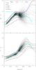Fig. 1 SDSS g − r and r − i colours versus redshift for the LRG sample used in this work. The solid cyan line indicates the median. The other lines show a range of Bruzual & Charlot (2003) SSP models, for various formation times (different colours) and metallicities (different line-styles) as indicated in the top-left of the figure.

In Fig. 2 we show the k-correction that these GALAXEV models predict, together with the k-correction for the LRGs that have been computed using KCORRECT. At z< 0.4, the Z = 0.02 tracks agree well, but at higher redshifts the k-correction values from KCORRECT are somewhat lower than those from the GALAXEV model. In fact, the agreement at 0.4 <z< 0.7 with the Z = 0.008 metallicity models is remarkable, but the validity of these models for our LRGs at low redshift is excluded based on the colour evolution in Fig. 1. However, at z> 0.4 the LRGs show an increasing scatter in their colours and become more compatible with the Z = 0.008 models.

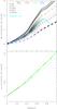Fig. 2 Top panel: k-correction as a function of redshift. The gray scale shows the k-corrections from the KCORRECT code, the solid cyan line indicates the median and the other coloured lines show the k-correction as predicted by a range of Bruzual & Charlot (2003) SSP models, for various formation times (different colours) and metallicities (different line-styles) as indicated in the top-left of the figure. Bottom panel: luminosity evolution correction as a function of redshift. For clarity, we only show a few of the Bruzual & Charlot (2003) model predictions. The thick green dot-dot-dashed line shows the correction we have used in this work, which is based on the Z = 0.02 instantaneous-burst model that formed 11 Gyr ago.

We show the luminosity evolution of some of the GALAXEV models in Fig. 2. We only show the models with Z = 0.02 and Z = 0.008, because the models with different metallicities were excluded based on their colour evolution and k-corrections. In addition, we only show models with a formation time of 10, 11 and 12 Gyr, as most previous works on the luminosity evolution of LRGs have adopted a formation time in this range (e.g. Wake et al. 2006; Maraston et al. 2009; Banerji et al. 2010; Carson & Nichol 2010; Liu et al. 2012). For our nominal luminosity evolution correction, we adopted the Z = 0.02 model that formed 11 Gyr ago (at redshift 0). Because none of the models exactly captures the trends in Figs. 1 and 2, the evolution correction we used may have a small bias. However, we have also tried different evolution corrections with corresponding models that broadly cover the observed colour evolution and k-correction values. We report on this test in Sect. 4.1; the main result is that our results do not change significantly. This suggests that the systematic bias in the luminosities caused by an incorrect evolution correction is probably insignificant for this work.

LRGs have formed over a certain range of time and with some range of metallicities. Hence their actual luminosity evolution corrections may have some scatter compared to our nominal correction, as we found that the luminosity evolution correction is increasingly sensitive with redshift to these parameters. If this scatter is random with respect to our nominal correction, this causes an Eddington bias, as lenses are preferentially scattered to where there are fewer of them. In Appendix A, we estimate the effect this may have on our mass estimates. We find that it is significantly smaller than our statistical errors and can be safely ignored.

In Fig. 3, we show the distribution of absolute magnitudes after including the k-correction and the (k + e)-correction. In the range 0.15 <z< 0.65 the distribution of k + e corrected absolute magnitudes is fairly flat. At redshifts z< 0.15 we have a tail of fainter objects in our catalogues, which are probably different types of galaxies. Therefore, we excluded them from this analysis. At higher redshifts, we start loosing fainter objects due to incompleteness. Since we determined both the mean luminosity and the mean halo mass for a given lens sample, this should not bias the overall mass-to-luminosity relation.

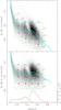Fig. 3 Distribution of absolute magnitudes and redshifts of our LRG lenses after the k-correction (top) and after the k-correction and luminosity evolution correction (bottom). The solid cyan line indicates the median. The green dashed boxes show the redshift and luminosity cuts on our lens sample; the magenta pentagons indicate the mean redshift and luminosity of those bins. The total density of LRGs as a function of redshift is shown by the black and red histograms on the horizontal axis for the LOWZ and CMASS galaxies, respectively.

2.2. Lensing measurement

The shapes of the background galaxies were measured on images from the RCS2. Details on the data reduction and the shape measurement process can be found in van Uitert et al. (2011), and some important improvements of our lensing analysis were discussed in Cacciato et al. (2014). It suffices to say that we measured the shapes of the galaxies with the KSB method (Kaiser et al. 1995; Luppino & Kaiser 1997; Hoekstra et al. 1998), using the implementation described by Hoekstra et al. (1998, 2000). This method was tested on a range of simulations as part of the Shear Testing Programme (STEP) 1 and 2 (the “HH” method in Heymans et al. 2006 and Massey et al. 2007, respectively), where it was found to have a multiplicative bias of a few per cent at most and a negligible additive bias. Recently, Hoekstra et al. (2015) found that these results were driven by the overly simplistic nature of the STEP simulations; for more realistic simulations, KSB suffers from noise bias (Kacprzak et al. 2012; Melchior & Viola 2012; Refregier et al. 2012) as any other shape measurement method that is currently in use. We calibrated our KSB implementation on realistic image simulations generated with GalSim² (Rowe et al. 2014) that are set up to closely match RCS2 observations, that is, with an intrinsic ellipticity distribution that matches the observations, a realistic range of Sérsic profile indices for the simulated galaxies, and up to a magnitude limit that matches the RCS2. We determined the multiplicative bias as a function of seeing: ${\mathit{m}}_{\mathrm{corr}}\mathrm{=}\mathrm{-}\mathrm{0.065}\mathrm{\times }\mathrm{(}\mathit{FWHM}\mathrm{-}{\mathrm{0.7}}^{\mathrm{\prime \prime }}\mathrm{)}\mathrm{-}\mathrm{0.123}\mathit{,}$(1)with FWHM the size of stars in an image. We used this to correct the shear measured in each RCS2 image. We did not need to correct for residual additive bias as that generally averages out in galaxy-galaxy lensing as a result of symmetry in lens-source pair orientations. The (multiplicative) noise bias correction increases the average lensing signal by 10–15%. Note that the correction is not very sensitive to the adopted width of the intrinsic ellipticity distribution, but that it is critically important to include simulated galaxies up to ~1.5 mag deeper than the nominal magnitude limit of the survey (see Hoekstra et al. 2015).

The lensing signal was extracted by azimuthally averaging the tangential projections of the ellipticities of the source galaxies in concentric radial bins, that is, by measuring the tangential shear as a function of projected separation: 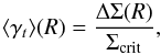$\mathrm{⟨}{\mathit{\gamma }}_{\mathit{t}}\mathrm{⟩}\mathrm{\left(}\mathit{R}\mathrm{\right)}\mathrm{=}\frac{\mathrm{\Delta \Sigma }\mathrm{\left(}\mathit{R}\mathrm{\right)}}{{\mathrm{\Sigma }}_{\mathrm{crit}}}\mathit{,}$(2)where 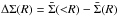is the difference between the mean projected surface density inside radius R and the projected surface density at R, and Σ_crit is the critical surface density: 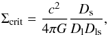${\mathrm{\Sigma }}_{\mathrm{crit}}\mathrm{=}\frac{{\mathit{c}}^{\mathrm{2}}}{\mathrm{4}\mathit{\pi G}}\frac{{\mathit{D}}_{\mathrm{s}}}{{\mathit{D}}_{\mathrm{l}}{\mathit{D}}_{\mathrm{ls}}}\mathit{,}$(3)with D_l, D_s, and D_ls the angular diameter distance to the lens, the source, and between the lens and the source, respectively. All galaxies with an apparent magnitude of 22 <r′< 24 and a well-defined shape measurement were selected as sources.

We measured the lensing signal from the BOSS lenses in each 1 × 1 deg² RCS2 pointing, including the sources from the neighbouring pointings (if present). We bootstrapped over these patches to obtain the covariance matrix, which accounts for intrinsic shape noise, measurement noise, and the contribution from large-scale structures. The off-diagonal elements are consistent with zero on the radial range of interest (<$\mathrm{2}\hspace{0.17em}{\mathit{h}}_{\mathrm{70}}^{-1}$ Mpc), hence we only used the inverse of the diagonal as the errors on the measurement when fitting the models to the data.

As these patches overlap, the contribution from large-scale structures might be somewhat underestimated at large scales; therefore, as a test, we also performed the lensing measurements on 2 × 2 deg² non-overlapping patches and used that in the bootstrap resampling. The resulting signal and covariance matrix barely change in the radial range that we used in this work. Since the total area decreases if we limit our analysis to 2 × 2 deg² non-overlapping patches only, and since it makes no difference to the signal and its error, we decided to use all 1 × 1 deg² RCS2 pointings plus neighbours as basis for the bootstrapping.

To compute Σ_crit we need the distances to the lenses and sources. We computed D_l for each lens separately using its spectroscopic redshift from SDSS. The lensing efficiencies ⟨ D_ls/D_s ⟩ were determined by averaging over the source redshift distribution, which was obtained by applying the same r′-band selection to the publicly available photometric redshift catalogues of the COSMOS field from Ilbert et al. (2013). The procedure is described in more detail in Appendix C of Cacciato et al. (2014). Note that we previously used the photometric redshift catalogues from Ilbert et al. (2009) as the former was not yet publicly available. The average lensing efficiencies from the two catalogues agree for low lens redshifts, but they are increasingly different at higher redshifts (up to 15% at z_l = 0.7). At increasingly high lens redshift the lensing efficiencies are more sensitive to the form of the adopted source redshift distribution, which is somewhat different for the two catalogues. We discuss the robustness of the derived lensing efficiencies in more detail in Appendix B.

A fraction of the sources is physically associated with the lens galaxies, representing an overdensity of source galaxies that are not lensed. We cannot remove them since we lack redshifts for our sources. Such a contamination in the source catalogue dilutes the lensing signal. This can be corrected for by measuring the excess source number density relative to the background as a function of projected separation and boosting the lensing signal with this factor (e.g. Mandelbaum et al. 2006b; van Uitert et al. 2011). We followed this procedure.

This boost correction itself is biased low as the galaxies associated with the lens, and the lens itself, block light from the background sky, suppressing the source number density. The effect is described in Simet & Mandelbaum (2014). As discussed in that work, a correction for this bias is obtained by multiplying the boost correction with a factor 1/(1−f_obsc), where f_obsc is the fraction of the sky that is obscured by the foreground galaxies. We computed this by using the ISOAREA_IMAGE keyword in SExtractor, which stores how many pixels a galaxy spans on the sky. f_obsc is taken to be the sum of these values of all galaxies whose centroids fall inside a radial bin, divided by the total number of pixels in that bin (accounting for the effect of the survey masks and geometry). Before correcting, we subtracted the average sky-background of f_obsc from the one observed around the lenses, as we are only interested in the additional obscuration. The correction is at most 5% in the radial bins closest to the most luminous and low-redshift lenses. It decreases at larger radii, as well as for fainter, higher redshift LRGs, as expected.

The robustness of the lensing signal has been addressed in Appendix B of Cacciato et al. (2014). There, we showed that the cross shear signal of our lens sample is consistent with zero. The random shear signal that was used to correct for the effect of residual systematics in the shape measurement catalogues is also weaker than the real signal for all the projected separations we use in this work. However, an overall multiplicative bias might still be present, either through an incorrect determination of the noise bias correction, or through the use of incorrect lensing efficiencies. In Appendix B we perform an internal consistency check of our measurement pipeline, which provides strong evidence that such a bias is probably not significant.

3. Halo model

In this section we describe the model that we employed to provide a physical interpretation of our measurements. The halo model provides a useful framework in which to describe the stacked weak-lensing signal around galaxies (see e.g. Mandelbaum et al. 2006b; Cacciato et al. 2009, 2014; Miyatake et al. 2015). It is based on a statistical description of dark matter properties, such as their average density profile, their abundance, and their large-scale bias, complemented with a statistical description of the way galaxies of a given luminosity populate dark matter haloes of different masses (also known as halo occupation statistics). In its fundamental assumptions, the model is similar to the one presented in Seljak (2000), Cooray & Sheth (2002) and Cacciato et al. (2009).

Galaxy-galaxy lensing probes the average matter distribution projected along the line of sight at a given projected physical separation, R, for a set of lenses. The quantity of interest is the excess surface mass density profile, ΔΣ(R), which is determined from the projected surface mass density, Σ(R). Since we measured the average signal of many lenses, the projected matter density can be expressed in terms of the galaxy-dark matter cross-correlation, ξ_gm(r): $\mathrm{\Sigma }\mathrm{\left(}\mathit{\theta }\mathrm{\right)}\mathrm{=}\mathit{\rho ̅}\mathrm{m}{\mathrm{\int }}_{\mathrm{0}}^{{\mathit{\omega }}_{\mathrm{s}}}\mathrm{[}\mathrm{1}\mathrm{+}{\mathit{\xi }}_{\mathrm{gm}}\mathrm{(}\mathit{r}{\mathrm{\left)}}^{\mathrm{\right]}}\mathrm{d}\mathit{\omega ,}$(4)where the integral is along the line of sight, ω is the comoving distance from the observer, ω_s the comoving distance to the source, and is the mean matter density at the redshift of the lens. The three-dimensional comoving distance r is related to ω through 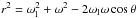${\mathit{r}}^{\mathrm{2}}\mathrm{=}{\mathit{\omega }}_{\mathrm{l}}^{\mathrm{2}}\mathrm{+}{\mathit{\omega }}^{\mathrm{2}}\mathrm{-}\mathrm{2}{\mathit{\omega }}_{\mathrm{l}}\mathit{\omega }\cos \mathit{\theta }$, with ω_l the comoving distance to the lens and θ = R/D_l the angular separation between lens and source (see Fig. 1 in Cacciato et al. 2009). Note that the cross-correlation of galaxy to dark matter is evaluated at the average redshift of the lens galaxies.

Under the assumption that each galaxy resides in a dark matter halo, ΔΣ can be computed using a statistical description of how galaxies are distributed over dark matter haloes of different masses (see e.g. van den Bosch et al. 2013). Specifically, it is fairly straightforward to obtain the two-point correlation function, ξ_gm(r,z), by Fourier-transforming the power-spectrum of galaxy to dark matter, P_gm(k,z), that is 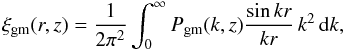$\begin{array}{ccc}{\mathit{\xi }}_{\mathrm{gm}}\mathrm{\left(}\mathit{r,z}\mathrm{\right)}\mathrm{=}\frac{\mathrm{1}}{\mathrm{2}{\mathit{\pi }}^{\mathrm{2}}}{\mathrm{\int }}_{\mathrm{0}}^{\mathrm{\infty }}{\mathit{P}}_{\mathrm{gm}}\mathrm{\left(}\mathit{k,z}\mathrm{\right)}\frac{\sin \mathit{kr}}{\mathit{kr}}\hspace{0.17em}{\mathit{k}}^{\mathrm{2}}\hspace{0.17em}\mathrm{d}\mathit{k,}& & \end{array}$(5)with k the wavenumber. The quantity P_gm(k,z) can be expressed as a sum of a term that describes the small scales (one-halo, 1h) and one that describes the large scales (two-halo, 2h), each of which can be further subdivided based upon the type of the galaxies (central or satellite) that contribute to the power spectrum. This reads ${\mathit{P}}_{\mathrm{gm}}\mathrm{\left(}\mathit{k}\mathrm{\right)}\mathrm{=}{\mathit{P}}_{\mathrm{cm}}^{\mathrm{1}\mathrm{h}}\mathrm{\left(}\mathit{k}\mathrm{\right)}\mathrm{+}{\mathit{P}}_{\mathrm{sm}}^{\mathrm{1}\mathrm{h}}\mathrm{\left(}\mathit{k}\mathrm{\right)}\mathrm{+}{\mathit{P}}_{\mathrm{cm}}^{\mathrm{2}\mathrm{h}}\mathrm{\left(}\mathit{k}\mathrm{\right)}\mathrm{+}{\mathit{P}}_{\mathrm{sm}}^{\mathrm{2}\mathrm{h}}\mathrm{\left(}\mathit{k}\mathrm{\right)}\hspace{0.17em}\mathit{.}$(6)The terms in Eq. (6) can be written in compact form as $\begin{array}{ccc}{\mathit{P}}_{\mathrm{xy}}^{\mathrm{1}\mathrm{h}}\mathrm{\left(}\mathit{k,z}\mathrm{\right)}& \mathrm{=}& \int {\mathrm{\mathscr{H}}}_{\mathrm{x}}\mathrm{\left(}\mathit{k,M,z}\mathrm{\right)}\hspace{0.17em}{\mathrm{\mathscr{H}}}_{\mathrm{y}}\mathrm{\left(}\mathit{k,M,z}\mathrm{\right)}\hspace{0.17em}{\mathit{n}}_{\mathrm{h}}\mathrm{\left(}\mathit{M,z}\mathrm{\right)}\hspace{0.17em}\mathrm{d}\mathit{M,}\\ {\mathit{P}}_{\mathrm{xy}}^{\mathrm{2}\mathrm{h}}\mathrm{\left(}\mathit{k,z}\mathrm{\right)}& \mathrm{=}& \int \mathrm{d}{\mathit{M}}_{\mathrm{1}}\hspace{0.17em}{\mathrm{\mathscr{H}}}_{\mathrm{x}}\mathrm{\left(}\mathit{k,}{\mathit{M}}_{\mathrm{1}}\mathit{,z}\mathrm{\right)}\hspace{0.17em}{\mathit{n}}_{\mathrm{h}}\mathrm{\left(}{\mathit{M}}_{\mathrm{1}}\mathit{,z}\mathrm{\right)}\\ & & \mathrm{\times }\mathrm{\int }\mathrm{d}{\mathit{M}}_{\mathrm{2}}\hspace{0.17em}{\mathrm{\mathscr{H}}}_{\mathrm{y}}\mathrm{\left(}\mathit{k,}{\mathit{M}}_{\mathrm{2}}\mathit{,z}\mathrm{\right)}\hspace{0.17em}{\mathit{n}}_{\mathrm{h}}\mathrm{\left(}{\mathit{M}}_{\mathrm{2}}\mathit{,z}\mathrm{\right)}\hspace{0.17em}\mathit{Q}\mathrm{\left(}\mathit{k}\mathrm{\right|}{\mathit{M}}_{\mathrm{1}}\mathit{,}{\mathit{M}}_{\mathrm{2}}\mathit{,z}\mathrm{)}\mathit{,} \end{array}$where x and y are either c (for central), s (for satellite), or m (for matter), $\mathit{Q}\mathrm{\left(}\mathit{k}\mathrm{\right|}{\mathit{M}}_{\mathrm{1}}\mathit{,}{\mathit{M}}_{\mathrm{2}}\mathit{,z}\mathrm{)}\mathrm{=}{\mathit{b}}_{\mathit{h}}\mathrm{(}{\mathit{M}}_{\mathrm{1}}\mathit{,z}\mathrm{\left)}{\mathit{b}}_{\mathit{h}}\mathrm{\right(}{\mathit{M}}_{\mathrm{2}}\mathit{,z}\mathrm{\left)}{\mathit{P}}_{\mathrm{m}}^{\mathrm{lin}}\mathrm{\right(}\mathit{k,z}\mathrm{)}$ describes the power spectrum of haloes of mass M₁ and M₂, and it contains the large-scale bias of haloes b_h(M) from Tinker et al. (2010; but see van den Bosch et al. 2013) for a more sophisticated modelling of this term). n_h(M,z) is the halo mass function of Tinker et al. (2010). Furthermore, we have defined ${\mathrm{\mathscr{H}}}_{\mathrm{m}}\mathrm{\left(}\mathit{k,M,z}\mathrm{\right)}\mathrm{=}\frac{\mathit{M}}{\mathit{\rho ̅}\mathrm{m}}\hspace{0.17em}\begin{array}{c}\mathrm{˜}\\ {\mathit{u}}_{\mathrm{h}}\end{array}\mathrm{\left(}\mathit{k}\mathrm{\right|}\mathit{M,z}\mathrm{)}\mathit{,}$(9)and ${\mathrm{\mathscr{H}}}_{\mathrm{x}}\mathrm{\left(}\mathit{k,M,z}\mathrm{\right)}\mathrm{=}\frac{\mathrm{⟨}{\mathit{N}}_{\mathrm{x}}\mathrm{|}\mathit{M}\mathrm{⟩}}{\mathit{n̅}\mathrm{x}\mathrm{\left(}\mathit{z}\mathrm{\right)}}\hspace{0.17em}{\begin{array}{c}\mathrm{˜}\\ \mathit{u}\end{array}}_{\mathrm{x}}\mathrm{\left(}\mathit{k}\mathrm{\right|}\mathit{M}\mathrm{)}$(10)where ${\begin{array}{c}\mathrm{˜}\\ \mathit{u}\end{array}}_{\mathrm{c}}\mathrm{\left(}\mathit{k}\mathrm{\right|}\mathit{M}\mathrm{)}\mathrm{=}\mathrm{1}\mathrm{-}{\mathit{p}}_{\mathrm{off}}\mathrm{+}{\mathit{p}}_{\mathrm{off}}\mathrm{\times }\exp \mathrm{[}\mathrm{-}\mathrm{0.5}{\mathit{k}}^{\mathrm{2}}\mathrm{(}{\mathit{r}}_{\mathit{s}}\mathrm{\left\{}\mathit{M}\mathrm{\right\}}{\mathrm{ℛ}}_{\mathrm{off}}{\mathrm{)}}^{\mathrm{2}}\mathrm{]}\mathit{,}$(11)and $\begin{array}{c}\mathrm{˜}\\ {\mathit{u}}_{\mathrm{s}}\end{array}\mathrm{\left(}\mathit{k}\mathrm{\right|}\mathit{M,z}\mathrm{)}\mathrm{=}\begin{array}{c}\mathrm{˜}\\ {\mathit{u}}_{\mathrm{h}}\end{array}\mathrm{(}\mathit{k}\mathrm{\left|}\mathit{M,z}\mathrm{\right)}\mathit{.}$(12)p_off is the parameter that describes the probability that the central galaxy does not reside at the centre of the dark matter halo, whereas ℛ_off quantifies the amount of off-centring in terms of the halo scale radius, r_s(M) (see e.g. Skibba et al. 2011; More et al. 2015). In our fiducial model, we set p_off = ℛ_off = 0, but we explore the impact of this assumption in Sect. 4. The functions ⟨ N_c | M ⟩ and ⟨ N_s | M ⟩ represent the average number of central and satellite galaxies in a halo of mass $\mathit{M}\mathrm{\equiv }\mathrm{4}\mathit{\pi }\mathrm{\left(}\mathrm{200}\mathit{\rho ̅}{}_{\mathrm{m}}\mathrm{\right)}{\mathit{R}}_{\mathrm{200}}^{\mathrm{3}}\mathit{/}\mathrm{3}$, defined as $\begin{array}{ccc}\mathrm{⟨}{\mathit{N}}_{\mathrm{c}}\mathrm{|}\mathit{M}\mathrm{⟩}& \mathrm{=}& \frac{\mathrm{1}}{\sqrt{\mathrm{2}\mathit{\pi }}\ln \mathrm{\left(}\mathrm{10}\mathrm{\right)}\mathit{M}{\mathit{\sigma }}_{\log \mathit{M}}}\\ & & \\ \mathrm{⟨}{\mathit{N}}_{\mathrm{s}}\mathrm{|}\mathit{M}\mathrm{⟩}& \mathrm{=}& \mathrm{(}\mathit{M}\mathit{/}{\mathit{M}}_{\mathrm{1}}\mathrm{)}\hspace{0.17em}{\mathit{f}}_{\mathrm{trans}}\mathrm{\left(}\mathit{M}\mathrm{\right)}\mathit{,}\end{array}$where ${\mathit{f}}_{\mathrm{trans}}\mathrm{\left(}\mathit{M}\mathrm{\right)}\mathrm{=}\mathrm{0.5}\mathrm{\times }\left[\mathrm{1}\mathrm{+}\mathrm{erf}\left(\frac{\log \mathit{M}\mathrm{-}\log {\mathit{M}}_{\mathrm{cut}}\mathrm{)}}{{\mathit{\sigma }}_{\mathrm{trans}}}\right)\right]\mathrm{·}$(15)We used a flat, non-informative prior for σ_log M and M_mean, set M_cut = ⟨ M_eff ⟩ (see Eq. (18)) and σ_trans = 0.25. Since LRGs are thought to be predominantly central galaxies (see e.g. Wake et al. 2008; Zheng et al. 2009; Parejko et al. 2013), we set ⟨ N_s | M ⟩ to zero and only fit for M_mean and σ_M in our nominal runs. We test the effect of this assumption on the derived quantities in the result sections by additionally fitting for M₁. We have tested that the result is fairly insensitive to the details of the modelling of f_trans(M).

is the number density of galaxies at redshift z: $\begin{array}{ccc}\mathit{n̅}\mathrm{g}\mathrm{\left(}\mathit{z}\mathrm{\right)}& \mathrm{=}& \int \mathrm{⟨}{\mathit{N}}_{\mathrm{g}}\mathrm{|}\mathit{M}\mathrm{⟩}{\mathit{n}}_{\mathrm{h}}\mathrm{(}\mathit{M,z}\mathrm{)}\mathrm{d}\mathit{M}\\ & \mathrm{\approx }& \mathrm{\int }\mathrm{⟨}{\mathit{N}}_{\mathrm{c}}\mathrm{|}\mathit{M}\mathrm{⟩}{\mathit{n}}_{\mathrm{h}}\mathrm{(}\mathit{M,z}\mathrm{)}\mathrm{d}\mathit{M}\mathit{.}\end{array}$(16)The last equality is exact if LRGs are only central galaxies. $\begin{array}{c}{}_{\mathrm{˜}}\\ {\mathit{u}}_{\mathrm{h}}\end{array}\mathrm{\left(}\mathit{k}\mathrm{\right|}\mathit{M,z}\mathrm{)}$ is the Fourier transform of the normalised density distribution of dark matter within a halo of mass M, for which we assume a Navarro-Frenk-White (NFW) profile (Navarro et al. 1996) and a mass-concentration relation from Duffy et al. (2008): ${\mathit{c}}_{\mathrm{m}}\mathrm{=}\mathit{A}{\left(\frac{\mathit{M}}{{\mathit{M}}_{\mathrm{pivot}}}\right)}^{\mathit{B}}\mathrm{(}\mathrm{1}\mathrm{+}\mathit{z}{\mathrm{)}}^{\mathit{C}}\mathit{,}$(17)with A = f_conc × 10.14, B = −0.081, C = −1.01, and M_pivot = 2 × 10¹² h^-1 M_⊙. Note that f_conc is a free parameter that allows the normalisation of this relation to vary. Specifically, we applied a non-informative flat prior on this parameter.

The average halo mass in a given luminosity bin, which we refer to as “effective” halo mass in what follows, can then be computed taking into account the weight of the halo mass function: $\mathrm{⟨}{\mathit{M}}_{\mathrm{eff}}\mathrm{⟩}\mathrm{=}\frac{\int \mathrm{⟨}{\mathit{N}}_{\mathrm{c}}\mathrm{|}{\mathit{M}}^{\mathrm{\prime }}\mathrm{⟩}{\mathit{n}}_{\mathrm{h}}\mathrm{(}{\mathit{M}}^{\mathrm{\prime }}\mathit{,}{\mathit{z}}_{\mathrm{lens}}\mathrm{)}{\mathit{M}}^{\mathrm{\prime }}\mathrm{d}\mathit{M}\prime }{\mathrm{\int }\mathrm{⟨}{\mathit{N}}_{\mathrm{c}}\mathrm{|}{\mathit{M}}^{\mathrm{\prime }}\mathrm{⟩}{\mathit{n}}_{\mathrm{h}}\mathrm{(}{\mathit{M}}^{\mathrm{\prime }}\mathit{,}{\mathit{z}}_{\mathrm{lens}}\mathrm{)}\mathrm{d}{\mathit{M}}^{\mathrm{\prime }}}\mathit{,}$(18)where z_lens is the mean redshift of the lens galaxies in a given luminosity bin. The distinction between the mass associated with the mean of the log-normal distribution and the halo mass inferred accounting for the mass function is of relevance because LRGs populate fairly massive haloes for which the mass function is steep (see e.g. Fig. 7 in Leauthaud et al. 2015).

At small scales one expects the baryonic mass of LRGs to contribute to the lensing signal. The smallest scale used in this study is 50 ${\mathit{h}}_{\mathrm{70}}^{-1}$ kpc, which is much larger than the typical extent of the baryonic content of a galaxy. Therefore, it is adequate to model the lensing signal of the LRGs itself as a point source of mass M_g ≈ M_∗. This reads $\mathrm{\Delta }{\mathrm{\Sigma }}^{\mathrm{1}\mathrm{h}\mathit{,}\mathrm{g}}\mathrm{\left(}\mathit{R}\mathrm{\right)}\mathrm{\approx }\frac{\mathrm{⟨}{\mathit{M}}_{\mathrm{\ast }}{\mathrm{⟩}}_{{\mathit{L}}_{\mathrm{-}}}^{{\mathit{L}}_{\mathrm{+}}}}{\mathit{\pi }\hspace{0.17em}{\mathit{R}}^{\mathrm{2}}}\mathrm{·}$(19)We used the value of the average stellar masses, ⟨ M_∗ ⟩, for the galaxies in the luminosity bins under investigation here. The stellar masses were obtained by matching our lens catalogue to the MPA-JHU stellar mass catalogue³. As the MPA-JHU catalogue is based on the MAIN sample from SDSS, we only have matches at low redshift. However, the point mass only has a weak effect on our fit results; hence we do not expect that a potential evolution of the average stellar mass-to-light ratio for LRGs can be so strong that it could significantly affect our results.

To summarise, our fiducial model for the lensing signal is the sum of three terms: one describing the lensing due to the baryonic mass; the second is responsible for the small-scale (sub-Mpc) signal mostly due to the dark matter density profile of haloes hosting central LRGs; and the last describes the large-scale (a few Mpc) signal due to the clustering of dark matter haloes around LRGs. This reads $\begin{array}{ccc}\mathrm{\Delta \Sigma }\mathrm{\left(}\mathit{R}\mathrm{\right)}& \mathrm{=}& \end{array}$(20)We simultaneously fitted the halo model to the three luminosity bins and did this for each redshift slice separately. We have five free parameters in each fit: the three mean masses of the luminosity bins, the scatter, and the normalisation of the mass-concentration relation. Since the scatter and the normalisation of the mass-concentration relation are fitted simultaneously to the three luminosity bins, the best-fit masses might be somewhat correlated. The fit was performed using a Markov chain Monte Carlo Method (MCMC). Details of its implementation can be found in Appendix C.

We fitted the model to the measurements on scales between 0.05 and 2 ${\mathit{h}}_{\mathrm{70}}^{-1}$ Mpc. At these scales, both the measured lensing signal and the halo model predictions are fairly robust. At larger scales, the lensing signal becomes weaker and more susceptible to residual systematics. At scales smaller than 0.05 ${\mathit{h}}_{\mathrm{70}}^{-1}$ Mpc, lens light may bias the shape measurements. For the halo model, the overlap between the one- and two-halo term is notoriously hard to model because of, amongst others, halo exclusion and non-linear biasing. This mainly affects the few-Mpc regime. Most of the information about the halo masses and concentrations is contained in the lensing signal within the virial radius, so we do not loose much statistical precision by limiting ourselves to these scales.

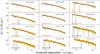Fig. 4 Lensing signal ΔΣ of LOWZ (top two rows) and CMASS (bottom two rows) lenses as a function of projected separation for the three luminosity bins (after the (k + e)-correction is applied). The solid red lines show the best-fit halo model, the orange and yellow regions the 1 and 2σ model uncertainty, respectively. We fit the signal on scales between 0.05 and 2 ${\mathit{h}}_{\mathrm{70}}^{-1}$ Mpc.

4. Luminosity-to-halo mass relation

To study how the luminosity-to-halo mass relation of LRGs evolves with redshift, we divided our sample into bins of (k + e)-corrected absolute magnitude and redshift as detailed in Table 1 and Fig. 3. For z< 0.43, we only selected lenses from the LOWZ sample, at higher redshifts we exclusively selected CMASS galaxies. The average log stellar masses for the consecutive luminosity bins are 11.2, 11.5, and 11.7 [$\log \mathrm{\left(}{\mathit{h}}_{\mathrm{70}}^{-2}{\mathit{M}}_{\mathrm{\odot }}\mathrm{\right)}$]. For each bin we measured the average lensing signal, which is shown in Fig. 4, together with the best-fit halo models and the model uncertainties (computed as detailed in Appendix C). The ${\mathit{\chi }}_{\mathrm{red}}^{\mathrm{2}}$ values are 1.8, 1.6, 1.2, and 1.0, going from the lowest to the highest redshift slice. Hence the fits of the CMASS samples are good, but for the LOWZ samples the ${\mathit{\chi }}_{\mathrm{red}}^{\mathrm{2}}$ values are somewhat high, suggesting that either our error bars are underestimated, or that the model that we fit to the data is overly simplistic.

The errors on the lensing measurements account for intrinsic shape noise, measurement noise, and the impact of large-scale structures. We have, however, ignored some small sources of error, as their amplitude is much smaller than the statistical errors on the lensing signal: the error on the boost correction, which is typically a few percent at small scales; the error on the obscuration correction, which is even smaller; the error on determining the lensing efficiency, and the error on the multiplicative bias calibration, whose magnitudes are unknown but are probably of the order of a few percent. Combined, they might increase the errors by as much as ~10%, although the exact number is difficult to estimate reliably. If we were to increase our error bars by this amount, we would obtain ${\mathit{\chi }}_{\mathrm{red}}^{\mathrm{2}}$ values of 1.5, 1.4, 1.0, and 0.8, respectively. The fact, however, that we find reasonable ${\mathit{\chi }}_{\mathrm{red}}^{\mathrm{2}}$ values for the CMASS sample, but not for the LOWZ sample, suggests that a systematic underestimate of our errors is probably not the dominant cause.

Even though a visual inspection of the covariance matrix led us to believe that it is diagonal on scales <2 ${\mathit{h}}_{\mathrm{70}}^{-1}$ Mpc, there might be low-level off-diagonal terms present that, if included, would lower the ${\mathit{\chi }}_{\mathrm{red}}^{\mathrm{2}}$ values. This potentially affects the LOWZ results more, as the measurements have a higher signal-to-noise ratio and the covariance matrix is less noisy. To test this, we recomputed the ${\mathit{\chi }}_{\mathrm{red}}^{\mathrm{2}}$ values using the full covariance matrix, which we obtained from bootstrapping (see Sect. 2.2) for the best-fit models. Note that we only included the covariance between radial bins of a lens sample, but not the covariance between the radial bins of the different luminosity samples. If present, they would lower the ${\mathit{\chi }}_{\mathrm{red}}^{\mathrm{2}}$ values even more. The ${\mathit{\chi }}_{\mathrm{red}}^{\mathrm{2}}$ of the first redshift slice reduces to 1.6, while it does not change for the other three redshift slices. Hence the effect is weak and does not fully explain the high ${\mathit{\chi }}_{\mathrm{red}}^{\mathrm{2}}$ values.

Figure 4 shows that the signal-to-noise ratio of the lensing measurements of the LOWZ samples is very high and would allow for a more sophisticated modelling. When we include a satellite term or a miscentering term in the halo model, however, the ${\mathit{\chi }}_{\mathrm{red}}^{\mathrm{2}}$ values do not improve, because the lensing signal alone cannot constrain the miscentring distribution parameters very well, and the expected number of satellites is low. Allowing for even more freedom in the fit might lead to overfitting of the CMASS results. Using different halo models for the different samples, or splitting the LOWZ sample up into more luminosity bins, reduces the homogeneity of the analysis, which is one of the key advantages of our work. Hence we chose to retain the settings described above. In Sect. 4.1 we perform a sensitivity analysis that shows that our results do not critically depend on various choices in the analysis, suggesting that the quantities we derive from the fits are robust.

In the halo model, we fit the mean and the scatter of the log-normal distribution that describes ⟨ N_c | M ⟩. The log of the mean has typical values of ~14.5, ~15 and ~15.5 for the three luminosity bins, while the scatter ranges between 0.7 and 0.8. Neither evolves with redshift. Note that this is the scatter in the log of the halo mass and not in luminosity. The latter was fit in Cacciato et al. (2014), where it was found to have a value of σ_log Lc = 0.146 ± 0.011, obtained by fitting the halo model to the lensing signal of all galaxies in the DR9 that overlap with RCS2. The scatter in halo mass is much larger because the luminosity-to-halo mass relation flattens at higher luminosities; a small scatter in luminosity corresponds to a large one in halo mass (see e.g. Fig. 3 and the discussion in More et al. 2009).

The quantity of interest that we can compare to other works is the effective halo mass, which is given in Table 1. We plot it as a function of luminosity in Fig. 5. Note that some correlation between the best-fit masses may exist because we simultaneously fit the scatter and the normalisation of the mass-concentration relation to the three luminosity bins. The masses increase with luminosity and decrease with redshift. To quantify this, we parametrised the luminosity-to-halo mass relation by M_eff = M_0,L(L/L₀)^β_L, using a pivot luminosity of ${\mathit{L}}_{\mathrm{0}}\mathrm{=}{\mathrm{10}}^{\mathrm{11}}{\mathit{h}}_{\mathrm{70}}^{-2}{\mathit{L}}_{\mathrm{\odot }}$. The best-fit power-law fits are shown in the same figure; the confidence contours of the fitted amplitude and slope are shown in Fig. 6. We have listed the fit parameters in Table 2.

The slope of the luminosity-to-halo mass relation does not change significantly for our different redshift samples and has a typical value of 1.4. The amplitude, however, is about ~4σ higher for our lowest redshift slice compared to the highest one. On average, the masses of LOWZ galaxies increase by $\mathrm{2}{\mathrm{5}}_{-14}^{\mathrm{+}\mathrm{16}}$% between redshift 0.36 and 0.22; the masses of CMASS galaxies increase by $\mathrm{1}{\mathrm{0}}_{-20}^{\mathrm{+}\mathrm{25}}$% from redshift 0.6 to 0.5. If we assume that CMASS galaxies evolve into LOWZ galaxies and combine the results, we find an average increase of $\mathrm{8}{\mathrm{0}}_{-28}^{\mathrm{+}\mathrm{39}}$% (stat. errors) in M_eff at ${\mathit{L}}_{\mathrm{0}}\mathrm{=}{\mathrm{10}}^{\mathrm{11}}{\mathit{h}}_{\mathrm{70}}^{-2}{\mathit{L}}_{\mathrm{\odot }}$ from z ~ 0.6 to z ~ 0.2. Fixing the slope to its average value of 1.4 and only fitting the amplitude changes this number to $\mathrm{7}{\mathrm{7}}_{-27}^{\mathrm{+}\mathrm{36}}$%.

We have ignored the correlation between the effective masses when computing the growth. This does not affect the average growth rate, but it can somewhat underestimate the error bars. As an extreme test, we have checked that if we assume a complete correlation of the effective masses in each redshift slice (thus grossly overestimating the expected effect), the halo mass growth for LRGs from z = 0.6 to z = 0.2 is $\mathrm{8}{\mathrm{0}}_{-43}^{\mathrm{+}\mathrm{67}}$%.

Tojeiro et al. (2012) found that at brighter absolute magnitudes, a larger portion of CMASS galaxies are the progenitors of LOWZ galaxies. If we discard the lowest luminosity bin, we find that for a pivot luminosity of ${\mathit{L}}_{\mathrm{0}}\mathrm{=}\mathrm{1.3}\mathrm{\times }{\mathrm{10}}^{\mathrm{11}}{\mathit{h}}_{\mathrm{70}}^{-2}{\mathit{L}}_{\mathrm{\odot }}$, the average halo mass increases with $\mathrm{9}{\mathrm{7}}_{-38}^{\mathrm{+}\mathrm{52}}$%. Considering only the brightest luminosity bin, the average halo mass increases with $\mathrm{16}{\mathrm{0}}_{-76}^{\mathrm{+}\mathrm{133}}$%.

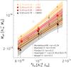Fig. 5 Mean (k + e)-corrected luminosity versus the best-fit halo mass of the twelve lens samples. The different symbols indicate the different redshifts bins, as indicated in the figure. The coloured areas indicate the 68% confidence intervals of the power-law fits.

Fig. 6 68% confidence contours for two parameters of the power-law fit between luminosity and halo mass.

4.1. Sensitivity analysis

To study how sensitive our results are to the adopted luminosity evolution correction, we performed the following test. We multiplied our nominal correction with a factor such that the resulting luminosity evolution curves roughly cover the range of reasonable models that are shown in the lower panel of Fig. 2. The factors we chose are 1−0.2 × z and 1 + 0.2 × z, respectively. Next, we recomputed the luminosities, repeated the lensing measurements (using the same cuts) and the halo model fits, and compared the resulting best-fit halo masses. The best-fit halo masses of the individual luminosity bins do not significantly shift compared to the nominal results. We fitted the luminosity-to-halo mass relation and list the parameters in Table 2. As is shown there, the best-fit slopes are very similar. The best-fit amplitude shifts with 1σ at most compared to our nominal results. For the 1−0.2 × z modification factor, the resulting increase in halo mass of LRGs from z = 0.6 to z = 0.2 is $\mathrm{8}{\mathrm{5}}_{-30}^{\mathrm{+}\mathrm{43}}$%; for the 1 + 0.2 × z modification factor, it is $\mathrm{5}{\mathrm{0}}_{-23}^{\mathrm{+}\mathrm{30}}$%. The halo masses and corresponding growth change somewhat because the lens selection shifts systematically, such that we analyse lens samples that to some extent are intrinsically different. Importantly, however, our results do not critically depend on the choice of the luminosity evolution correction. For future work that is expected to have an improved statistical precision, more detailed knowledge of this correction will be required.

To test how sensitive our results are to the assumption that all LRGs are located at the centre of their dark matter haloes, we performed two halo model runs where we allowed for more flexibility. First, we assumed that a fraction of the LRGs is miscentred, following Eq. (11). We used p_off and R_off as additional free parameters with a flat uninformative prior in the range [0,1]. The allowed miscentring distribution ranges from the lenses being all correctly centred (p_off = R_off = 0) to all being miscentred and located at the halo scale radius (p_off = R_off = 1). We find ${\mathit{p}}_{\mathrm{off}}\mathrm{=}\mathrm{0.5}{\mathrm{7}}_{-0.37}^{\mathrm{+}\mathrm{0.29}}$, $\mathrm{0.2}{\mathrm{6}}_{-0.23}^{\mathrm{+}\mathrm{0.39}}$, $\mathrm{0.5}{\mathrm{0}}_{-0.36}^{\mathrm{+}\mathrm{0.37}}$ and $\mathrm{0.4}{\mathrm{0}}_{-0.30}^{\mathrm{+}\mathrm{0.38}}$ for the low- and high-redshift bins of LOWZ and CMASS, respectively, with corresponding miscentring radii of ${\mathit{R}}_{\mathrm{off}}\mathrm{=}\mathrm{0.3}{\mathrm{7}}_{-0.25}^{\mathrm{+}\mathrm{0.41}}$, $\mathrm{0.3}{\mathrm{2}}_{-0.29}^{\mathrm{+}\mathrm{0.53}}$, $\mathrm{0.4}{\mathrm{9}}_{-0.37}^{\mathrm{+}\mathrm{0.39}}$ and $\mathrm{0.5}{\mathrm{4}}_{-0.43}^{\mathrm{+}\mathrm{0.37}}$. The resulting power-law parameters are listed in Table 2. They do not change significantly. The total increase in halo mass of LRGs corresponds to $\mathrm{7}{\mathrm{5}}_{-27}^{\mathrm{+}\mathrm{38}}$%, consistent with our nominal result of $\mathrm{8}{\mathrm{0}}_{-28}^{\mathrm{+}\mathrm{39}}$%. These constraints on the miscentring distribution broadly agree with previous galaxy-galaxy lensing and clustering results of CMASS galaxies. For instance, Miyatake et al. (2015) reported p_off< 0.66 and ${\mathit{R}}_{\mathrm{off}}\mathrm{=}\mathrm{0.7}{\mathrm{9}}_{-0.38}^{\mathrm{+}\mathrm{0.58}}$, whereas More et al. (2015) found p_off = 0.34 ± 0.18 and ${\mathit{R}}_{\mathrm{off}}\mathrm{=}\mathrm{2.}{\mathrm{2}}_{-1.3}^{\mathrm{+}\mathrm{1.5}}$.

As a related test, we studied how our results changed when we assumed that a fraction of LRGs are satellites. We used a simple model with only one free parameter, that is, M₁. We followed this approach because we are not interested in determining the satellite HOD (as lensing alone is not very sensitive to this), but because we wish to obtain an estimate of how strongly our results might be affected by ignoring the contribution of satellites. The typical satellite fraction for LRGs is ~10% and decreases for more massive LRGs (White et al. 2011; Parejko et al. 2013; More et al. 2015). We therefore set a prior on M₁ such that the resulting satellite fractions from our model are between 5% and 15%. The resulting luminosity-to-halo mass relation parameters are listed in Table 2. The best-fit slopes are consistent with our nominal run, but the amplitude decreases by 1-2σ. The total increase of halo mass is $\mathrm{8}{\mathrm{2}}_{-29}^{\mathrm{+}\mathrm{35}}$% over the full redshift range of our LRG sample, consistent with our nominal result. The normalisation decreases because the satellites are associated with more massive haloes, with correspondingly stronger lensing signals. This lowers the required contribution to the total signal from central LRGs, and hence their mass. This does not occur in the miscentring run, where the lensing signal is merely smeared out, but the integrated signal (and hence the mass) stays the same.

4.2. Comparison to previous work

Several previous works have provided mass estimates of LRGs, using gravitational lensing, clustering, abundance matching, or a combination of these. The selection of the samples, the models fit to the data, and the definitions of mass generally differ between these studies, which limits the level of detail with which we can perform a comparison.

4.2.1. Lensing results

Mandelbaum et al. (2006a) measured the masses for a sample of over 4 × 10⁴ LRGs with spectroscopic redshifts from SDSS-I/II using weak lensing. Bluer and fainter LRGs were discarded using colour-magnitude cuts, as well as LRGs that probably were satellites of larger systems, hence the selection is not identical to ours. The resulting sample was split into a faint and bright part using a cut at M_r = −22.3, and the mean luminosity of the two samples is 5.2 × 10¹⁰ and 8.6 × 10¹⁰ h^-2L_⊙, respectively. The luminosities were computed in a similar manner as in our work. All LRGs were selected in the redshift range 0.15 <z< 0.35 and have a mean effective redshift of 0.24. Masses were estimated using NFW fits plus a baryonic component, where the fitting range was restricted to small scales were the two-halo term can be neglected. The masses were defined as the enclosed mass in a sphere where the density is 180 times the mean background density, M_180b, instead of 200 times the mean density that we used; the difference between these definitions is only a few percent. The faint LRGs were found to reside in haloes of masses 2.9 ± 0.4 × 10¹³ h^-1 M_⊙ and the bright ones in haloes of masses 6.7 ± 0.8 × 10¹³ h^-1 M_⊙. The measurements are shown in Fig. 5. The masses of our low-redshift slices are substantially higher than the masses from Mandelbaum et al. (2006a). The discrepancy may be caused by the scatter between luminosity and halo mass, which was not included in Mandelbaum et al. (2006a). Allowing for a non-zero scatter results in higher halo masses.

Miyatake et al. (2015) measured the lensing signal of 4807 CMASS galaxies with 0.47 <z< 0.59 in the overlap with CFHTLS using the publicly available CFHTLenS catalogues (Heymans et al. 2012). The lensing signal was fitted together with the projected clustering signal using a halo model that is similar to the one we have adopted here. Halo masses were defined with respect to 200 times the background density, as we did. The average halo mass of CMASS galaxies was found to be 2.3 ± 0.1 × 10¹³ h^-1 M_⊙. To compare it with our results, we computed the average luminosity of CMASS galaxies with 0.47 <z< 0.59 in our catalogue. We find a value of 3.8 × 10¹⁰ h^-2L_⊙ and assume that this number is representative for the average luminosity of the lenses in that work. This estimate is slightly too low, as Miyatake et al. (2015) also applied a cut on stellar mass to remove the least massive (hence faintest) objects, which we cannot mimic. However, as an indication, if we remove the faintest 10% of our CMASS sample, the average luminosity only increases to 4.1 × 10¹⁰ h^-2L_⊙, hence it is unlikely that the average luminosity is far from the real value. We compare the results in Fig. 5 and find that our CMASS masses are somewhat lower but consistent.

Several papers have studied how the average mass of galaxies changes as a function of redshift (e.g. van Uitert et al. 2011; Choi et al. 2012; Leauthaud et al. 2012; Tinker et al. 2013; Hudson et al. 2015), using weak-lensing measurements. Since these works did not specifically target LRGs, and since the modelling of the signal differs from our approach, we cannot compare the results in detail. However, both Tinker et al. (2013) and Hudson et al. (2015) included red, massive galaxies in their work, hence we can at least compare the recovered trends.

Tinker et al. (2013) used measurements of weak lensing, clustering, and the stellar mass function of galaxies in COSMOS to constrain the stellar-to-halo mass relation. Halo masses were defined in the same way we did. The relations they report predict the average log ₁₀(M_∗) as a function of halo mass, instead of the average halo mass at a given stellar mass, which is what we measure; these relations are different as a result of intrinsic stellar mass scatter, which is illustrated in their Fig. 7. From the right-hand panel of that figure we observe that at the average stellar masses of our samples, the mean halo mass for passive galaxies is roughly ~0.5 dex lower than what we find. There are many differences between the analyses that could contribute to this difference, such as systematic offsets between stellar mass estimates, the selection of the samples, and the modelling of the signal. Nonetheless, at a stellar mass of log ₁₀(M_∗) ~ 11.4 (typical for LRGs), the average halo mass increases from ~10^12.9 to ~10^13.2 M_⊙ between redshifts of 0.88 and 0.36, an increase of almost 100%, similar to the average growth in halo mass that we find for our LRG sample from redshift 0.62 to 0.21.

Hudson et al. (2015) used the shape measurements from CFHTLenS to measure the lensing signal for blue and red galaxies in three redshift slices. The lenses were binned according to luminosity rather than stellar mass to avoid an Eddington bias due to the larger observational errors on stellar mass compared to luminosity. The stellar mass was then determined using the mean stellar-mass-to-luminosity ratio. For the highest luminosity bin of red lenses, which has a mean stellar mass of ~$\mathrm{2}\hspace{0.17em}\mathrm{\times }\hspace{0.17em}{\mathrm{10}}^{\mathrm{11}}{\mathit{h}}_{\mathrm{70}}^{-2}{\mathit{M}}_{\mathrm{\odot }}$, the average halo mass increases from $\mathrm{0.84}\mathrm{\pm }\mathrm{0.17}\mathrm{\times }{\mathrm{10}}^{\mathrm{13}}{\mathit{h}}_{\mathrm{70}}^{-1}{\mathit{M}}_{\mathrm{\odot }}$ to $\mathrm{1.32}\mathrm{\pm }\mathrm{0.33}\mathrm{\times }{\mathrm{10}}^{\mathrm{13}}{\mathit{h}}_{\mathrm{70}}^{-1}{\mathit{M}}_{\mathrm{\odot }}$ from redshift 0.67 to 0.29. The masses were defined with respect to ρ_crit instead of the mean density, resulting in masses that are ~30–40% lower compared to ours. Furthermore, the intrinsic scatter between luminosity/stellar mass and halo mass was not accounted for in their modelling, which also leads to lower masses. Finally, the selection of the lens samples differs. However, the ~58% increase in average halo mass is similar to what we find.

4.2.2. Clustering results

The clustering of LRGs is widely studied in the literature and has been used to derive halo masses (e.g. Blake et al. 2008; Wake et al. 2008; Zheng et al. 2009; Sawangwit et al. 2011; Nikoloudakis et al. 2013; Parejko et al. 2013; Guo et al. 2014). Parejko et al. (2013) measured the clustering of galaxies with 0.2 <z< 0.4 from the LOWZ sample and fitted it with a halo model. The probability distribution of halo masses, as shown in their Fig. 9, has a mean of 5.2 × 10¹³ h^-1 M_⊙. We plot it in Fig. 5 and find that it is higher than our LOWZ measurements. Although not specified, we assume that the mass is defined as M_180b, as is mentioned in a companion paper (White et al. 2011), which is similar to our definition. Their halo mass distribution is fairly broad, however, and our constraints may well fall inside their 68% confidence region.

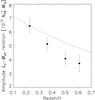Fig. 7 Evolution of the amplitude of the power-law fit between luminosity and halo mass with redshift. The black dashed lines shows the predicted trend from pseudo-evolution (Diemer et al. 2013) for halo masses that are typical for LRGs, scaled to overlap with our first data point.

Guo et al. (2014) measured the clustering of CMASS galaxies divided into three i-band-magnitude selected samples, which we cannot directly compare to our measurements. They reported that going from their faintest to their brightest bins, the peak host halo mass increases from 1.1 × 10¹³ h^-1 M_⊙ to 3.3 × 10¹³ h^-1 M_⊙, which is quite similar to our results. Their masses are defined with respect to the mean density, like ours. However, we measure an “effective” mass and not the peak halo mass, and it is unclear how much these definitions differ.

Zheng et al. (2009) fitted the clustering signal of SDSS-I/II LRGs using an HOD approach. Their LRGs are divided into a faint and bright sample using their M_g magnitude, hence we cannot directly compare. The distribution of halo masses (defined like ours) of these samples peaks at ~4.5 × 10¹³ h^-1 M_⊙ and ~10¹⁴ h^-1 M_⊙, respectively, similar to the values we find for faint and bright LOWZ samples, but note, again, that we measured the effective mass and not the peak halo mass. The scaling of luminosity with host halo mass, which is given by L_c ∝ M^0.66, is consistent with our results.

Wake et al. (2008) measured the evolution of the clustering signal of galaxies from SDSS and the 2dF-SDSS LRG and QSO Survey (2SLAQ; Cannon et al. 2006). They matched the selections using colour and magnitude cuts, which complicates the comparison with our results. However, they reported that the effective halo masses increased with ~50% from z = 0.55 to z = 0.2, consistent with our findings. Sawangwit et al. (2011) studied three separate LRGs samples in SDSS, with a mean redshift of 0.35, 0.55 and 0.75. After applying additional selection criteria such that the space density of LRGs is similar to the SDSS-I/II LRG sample, the effective halo mass, defined as the virial mass, is found to be 6.4 ± 0.5 × 10¹³ h^-1 M_⊙, 4.7 ± 0.2 × 10¹³ h^-1 M_⊙ and 4.3 ± 0.2 × 10¹³ h^-1 M_⊙, respectively. We assume that the average luminosity of these three samples is similar to that of the LOWZ sample and show their measurements in Fig. 5. Their results agree fairly well with ours. Blake et al. (2008) and Nikoloudakis et al. (2013) studied the clustering signal of different samples of LRGs, which is difficult to compare with our results. The typical halo masses of LRGs are found to be a few times 10¹³ h^-1 M_⊙, which broadly agrees with our results.

4.2.3. Abundance-matching results

Masaki et al. (2013) applied an abundance-matching technique to N-body simulations to construct mock LRG samples whose number density matched that of LRGs in SDSS. From these samples a mock lensing signal was constructed, whose shape agrees well with, but whose amplitude is ~20% larger than, the measured lensing signal of SDSS LRGs presented in Mandelbaum et al. (2013). Masaki et al. (2013) find that their LRGs reside in haloes with a mean virial mass of 5.6 ± 0.1 × 10¹³ h^-1 M_⊙. This definition of mass is ~10% lower than M₂₀₀ for masses and concentrations that are typical for LRGs at z ~ 0.3. We assume the average luminosity equals that of SDSS-I/II LRGs and show the measurement in Fig. 5. This mass estimate agrees fairly well with our results.

4.3. Interpretation

M_eff of LRGs increases by approximately 80% from redshift 0.6 to 0.2. This is not only because of dark matter accretion. Part of the growth can be attributed to the so-called pseudo-evolution (Diemer et al. 2013). M₂₀₀ is defined with respect to a reference density, which is redshift dependent. Even if a halo is static, that is, it does not accrete anything, M₂₀₀ increases towards lower redshift. The halo mass function that we used to determine M_eff uses masses that are defined with respect to ρ_m(z). Hence the evolution of the halo mass function is a mix of physical evolution and pseudo-evolution. Therefore, the evolution of M_eff is also a mix of the two.

Since the halo masses of our LRGs span a relatively narrow range, we can estimate the contribution from pseudo-evolution to our observed increase in mass using the results from Diemer et al. (2013). For halo masses that are typical for our LRGs, M₂₀₀ increases by approximately 33% from z = 0.6 to z = 0.2 due to pseudo-evolution, as is illustrated in Fig. 7. If we fit the amplitude of the pseudo-evolution curve to our measurements, we find that ${\mathit{\chi }}_{\mathrm{red}}^{\mathrm{2}}\mathrm{=}\mathrm{1.3}$, providing weak support that the slope is steeper and requires additional dark matter accretion.

It is interesting to compare our growth rates to those obtained from simulations. Ideally, we would like to compare to hydrodynamical simulations, but none are available for the mass range we are interested in. However, a comparison with dark-matter-only simulations is interesting as well because a good or poor agreement points towards the relevance of baryonic physics. We first compare our results to the two Millennium simulations, for which growth and merger rates have been derived in Fakhouri et al. (2010). These authors find that the growth rate is well described by 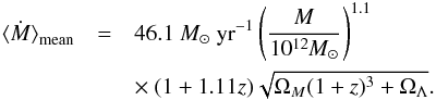$\begin{array}{ccc}\dot{\mathrm{⟨}\mathit{M}\mathrm{⟩}}\mathrm{mean}& \mathrm{=}& \mathrm{46.1}{\mathit{M}}_{\mathrm{\odot }}{\mathrm{yr}}^{-1}{\left(\frac{\mathit{M}}{{\mathrm{10}}^{\mathrm{12}}{\mathit{M}}_{\mathrm{\odot }}}\right)}^{\mathrm{1.1}}\\ & & \mathrm{\times }\mathrm{(}\mathrm{1}\mathrm{+}\mathrm{1.11}\mathit{z}\mathrm{)}\sqrt{{\mathrm{\Omega }}_{\mathit{M}}\mathrm{(}\mathrm{1}\mathrm{+}\mathit{z}{\mathrm{)}}^{\mathrm{3}}\mathrm{+}{\mathrm{\Omega }}_{\mathrm{\Lambda }}}\mathit{.}\end{array}$(21)Using this equation, we find that a halo of mass 10¹³ M_⊙ grows by 38% from redshift 0.6 to 0.22, whilst a halo of mass 5×10¹³ M_⊙ grows by 43%. More recently, Wetzel & Nagai (2014) used hydrodynamical simulations to measure the amount of physical accretion (i.e. after accounting for pseudo-evolution) for haloes with masses 10¹¹−10¹³ M_⊙. However, for masses in the range 10¹³−10¹⁴ M_⊙, which are typical for LRGs, they used dark-matter-only simulations and derived a growth of ~10% between z = 0.5 to z = 0 at scales smaller than a few hundred kpc. Together with pseudo-evolution, the total growth amounts to ~43%, which is similar to the results of Fakhouri et al. (2010).

Wetzel & Nagai (2014) only studied isolated haloes; LRGs cluster strongly, which means that the typical halo in that work may not be very representative for LRGs. However, no environment selection cuts were made in Fakhouri et al. (2010) and the derived growth rates are similar, hence this seems to be unimportant. In fact, Fakhouri & Ma (2010) measured the growth rate as a function of environment and found a weak trend of a decreasing growth rate towards denser environments, but the statistics for massive haloes is poor because they only had few of them.

The growth rates predicted from dark-matter-only simulations are marginally consistent with our results. Our measurements suggest a stronger growth, particularly towards more massive haloes. This could indicate the effect of baryons; particularly AGN feedback may have an effect on the distribution of matter in massive haloes (Duffy et al. 2010; Velliscig et al. 2014) and their accretion history. However, we need to improve the statistics of our measurements before we can make stronger claims.

Our conclusion about the evolution of the luminosity-to-halo mass relation depends on the validity of the assumption of pure passive evolution, however. The absence of a clear tilt in Fig. 3 supports this view. Nonetheless, some residual star formation and/or mergers may also affect the luminosities, which might affect our conclusions.

The colour evolution of LRGs shows that the amount of ongoing star formation is low (Wake et al. 2006; Maraston et al. 2009). Moreover, spectral analyses from SDSS-I/II LRGs and CMASS galaxies point toward a very low fraction of galaxies that either form stars or have AGN activity (Greisel et al. 2013; Thomas et al. 2013). There are indications that intermediate-mass early-type galaxies have a low level of ongoing star formation (e.g. Kaviraj et al. 2007; Schawinski et al. 2007; Salim & Rich 2010), but it seems unlikely that it is sufficiently strong to affect our conclusions.

Mergers also complicate a purely passive luminosity evolution scenario. The merging history of LRGs or massive early-type galaxies has received considerable attention in recent years (e.g. Tal et al. 2012; López-Sanjuan et al. 2012; Gabor & Davé 2012; Bédorf & Portegies Zwart 2013; Ruiz et al. 2014). We focus here on the results from Tojeiro & Percival (2010), because they estimated the amount of luminosity growth in LRGs due to mergers. Their analysis is based on the measured luminosity function and clustering strength of LRGs in the SDSS in the redshift range 0.15 <z< 0.5, from which they deduced that the average luminosity of LRGs increases by 1.5-6% Gyr^-1 due to mergers, depending on luminosity, such that the growth mainly occurs for the faintest LRGs. For LRGs with M_r,0.1< −22.8, the evolution is consistent with passive evolution. In Table 4 of that work, luminosity growth rates from recent works are compared; the results indicate that their values are fairly representative.

Tojeiro & Percival (2010) proposed two type of mergers that might contribute to the luminosity growth: a merger between an LRG and a small companion, or a merger between two small companions, whose combined luminosity is sufficient to classify it as LRG. In the first scenario, the luminosities of LRGs increase towards lower redshifts; hence they are overestimated compared to the luminosities of LRGs that have evolved through pure passive evolution.

To estimate how this might affect our derived luminosity-to-halo mass relations and their evolution, we assumed that the luminosities of our three LRGs samples increase through mergers with 2, 4, and 6% Gyr^-1, from the bright to the faint bin, respectively, without affecting the halo masses, that is, we assumed that the mass-to-light ratio of the smaller companions equals zero. This provided an upper limit on the bias in the derived halo mass growth. We used the highest redshift slice as our reference and lowered the luminosities of the lower redshift slices to mimic how the evolution would have looked in the absence of mergers. For example, between z = 0.6 and z = 0.2, approximately 3.3 Gyr passed, therefore we lowered the luminosity of the L1z1 bin by a factor 1.06^3.3 ≈ 1.2. We applied this factor to the average passively evolved luminosities, meaning that we did not apply it to the individual luminosities before the selection of the samples. After this adjustment, we fitted the luminosity-to-halo mass relation again. The retrieved slopes of the luminosity-to-halo mass relation are within the error bars of our nominal results. The amplitudes increase by ~2σ for our 0.15 <z< 0.29 redshift slice and by ~1σ for our 0.29 <z< 0.43 slice. The average growth in halo mass becomes $\mathrm{11}{\mathrm{6}}_{-35}^{\mathrm{+}\mathrm{50}}$%, consistent with our nominal result. We ignored here that mergers also cause growth in mass, hence the LRGs move diagonally rather than horizontally in the luminosity-to-halo mass plane. If the mass-to-light ratio of the smaller companions is similar to that of the LRG, they move along the luminosity-to-halo mass relation and no bias is caused; if this ratio is higher than that of LRGs, the actual growth in halo mass would be lower than our nominal value.

The second channel for luminosity growth through mergers described by Tojeiro is through the merging of two faint galaxies, which are individually not bright enough to be selected as an LRG. As the formation history differs from that of the typical LRG that formed at high redshift without much activity afterwards, the properties of their haloes may be different, which complicates the interpretation of the measured trends.

Apart from this, there are several other physical processes that complicate the interpretation. For example, star formation and mergers may be linked in LRGs (Kaviraj et al. 2011). In addition, some high-redshift LRGs may not become low-redshift LRGs, as they may be tidally disrupted or merge with other galaxies. Furthermore, AGN activity could trigger star formation, leading to too blue colours to match the LRG colour selection at lower redshift. The subset of LRGs whose luminosity-to-halo mass evolution is most easy to interpret is probably the brightest one: Tojeiro et al. (2012) reported that the brightest CMASS galaxies are most likely to evolve in SDSS-I/II LRGs, and Tojeiro & Percival (2010) derived that the brightest LRGs experience the least amount of luminosity growth from mergers.

To summarise: although passive evolution accounts for the bulk of the luminosity evolution of LRGs, there are several processes that complicate this picture. This affects our ability to select and compare LRGs and their progenitors at different redshifts. To extract the full information content on the evolution of LRGs that is contained in our measurements, it needs to be compared with numerical simulations that contain all relevant physical processes. No luminosity evolution correction needs to be applied in that case, since there is no need to match the samples at different redshifts, as long as the selection can be matched in observations and simulations. The range in luminosity and redshift of the LRG sample studied in this work would form an ideal observational test case for such a study.

5. Mass-concentration relation

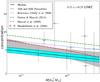Fig. 8 Best-fit mass-concentration relation derived for the 0.15<z<0.29 LOWZ bin. The solid black line indicates the best-fit result and the turquoise area the 68% confidence intervals. The blue dotted line shows the reference relation from Duffy et al. (2008), whose amplitude we fit in the halo model. The red and green dotted-dashed lines show the relations from Macciò et al. (2008) and Dutton & Macciò (2014), respectively. The black points and the grey area are the results from direct fits to lensing data from Mandelbaum et al. (2008).

As discussed in Sect. 3, we assumed a functional form for the mass-concentration relation, that is, the one from Duffy et al. (2008), but we allowed the overall normalisation of this relation to vary in the fit. The resulting constraints for the 0.15 <z< 0.29 LOWZ bins are shown in Fig. 8 together with the nominal Duffy et al. (2008) model. The constraints on f_conc as a function of redshift are shown in Fig. 9 and listed in Table 1.

The derived mass-concentration relations are lower than the reference model. The strongest discrepancy is for our lowest redshift slice, where we find ${\mathit{f}}_{\mathrm{conc}}\mathrm{=}\mathrm{0.6}{\mathrm{8}}_{-0.06}^{\mathrm{+}\mathrm{0.08}}$. For the other redshift slices, our results are about 1σ below the relation from Duffy et al. (2008). There is no evidence for a trend of f_conc with redshift, although the errors of the higher redshift bins are still fairly large. This suggests that the redshift scaling of this relation is well captured by its functional form (Eq. (17)).

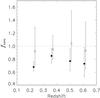Fig. 9 Best-fit normalisation of the mass-concentration relation from Duffy et al. (2008) for the four redshift slices. Filled symbols show the results for the nominal run, open symbols for the miscentring run. The open symbols have been shifted to the right for clarity.

In Fig. 8, we also plot the relation from Macciò et al. (2008), which is based on dark-matter-only simulations using the WMAP3 cosmology (Hinshaw et al. 2009), and the relation from Dutton & Macciò (2014), who derived the mass-concentration relation with N-body simulations using the Planck cosmology (Planck Collaboration XVI 2014). All the relations are shown for a redshift of 0.23. These relations derived from dark-matter-only simulations consistently predict higher concentrations in the mass range that we study.

It is possible that the low normalisation results from choices in our modelling. Therefore, we also derived the normalisation of the mass-concentration relation for the halo model runs where we either allowed a fraction of the LRGs to be miscentred, or where we allowed a non-zero satellite fraction. We also derived the normalisation for our alternative luminosity evolution correction runs. The results are listed in Table 2. For the alternative luminosity evolution run, the constraints on f_conc do not change significantly. For the other two runs, the normalisations increase and become consistent with unity, as is shown in Fig. 9. By adding either satellites or a miscentred component, we shifted power from small scales to intermediate scales. Consequently, to fit the same data, the lensing signal of the central LRGs needs to become steeper, that is, the concentrations need to increase. Note that the errors on f_conc increase as well as a result of the increased freedom in the model (particularly for the miscentring run).

In Fig. 8 we also show the results from Mandelbaum et al. (2008), who derived the mass-concentration relation by combining lensing measurements for L∗-type galaxies, galaxy groups traced by LRGs, and the maxBCG cluster sample in the SDSS. The model used for their main results did not include a miscentring component, but they used a minimum scale in the fit of 500 h^-1 kpc for the maxBCG sample to reduce the effect of miscentring. We only show the measurements that overlap with our range of halo masses. Our results are consistent with those of Mandelbaum et al. (2008). Towards lower masses, the mass-concentration relation of Mandelbaum et al. (2008) agrees with theoretical expectations, but at higher masses, the normalisation is lower, as can been seen in their Fig. 5. As their lenses span a broad range of masses, they can fit a more flexible mass-concentration relation to their measurements, which results in a broader confidence region than ours.

The mass-concentration relation of CMASS galaxies was also derived in Miyatake et al. (2015). Their results are very similar to ours: using their fiducial model, in which all galaxies are located at the centre of dark matter haloes, they found a normalisation of f_conc = 0.78 ± 0.12 with respect to the relation of Macciò et al. (2007). However, when they included a miscentring component identical to ours, the normalisation factor became consistent with unity.

The results from Miyatake et al. (2015) and the results presented here suggest that the low normalisation of the mass-concentration relation can be explained by allowing for satellites and/or a miscentring component in the modelling, although the constraints on the miscentring parameters are still very weak. To understand whether the effect is real, one either needs to employ larger datasets whose corresponding statistical errors are much smaller, or alternatively, use group catalogues with spectroscopically identified members to study the brightest group members and the satellites separately. The overlap between the Galaxy And Mass Assembly (GAMA; Driver et al. 2009, 2011; Robotham et al. 2011) and the Kilo Degree Survey (KiDS; Kuijken et al., in prep) could offer an excellent dataset for such a work.

However, it is interesting to consider alternative explanations, such as baryonic processes that can lower the concentrations. AGN feedback, for example, may affect the distribution of dark matter at the relevant radii, as has been studied in Velliscig et al. (2014). In that work, several baryonic processes such as cooling, supernova feedback, and AGN feedback were implemented in hydrodynamical simulations to study their effect on the density profiles of haloes. For halo masses typical for LRGs, AGN feedback is the dominant process and affects the dark matter distribution out to several times the virial radius, such that the density is lower at small scales. A similar conclusion was reached in Duffy et al. (2010); whilst cooling leads to more concentrated haloes, this effect is counteracted by AGN feedback, which could cause the concentrations to become lower by about 15% than those from dark-matter-only simulations.

6. Conclusion

We studied the evolution of the luminosity-to-halo mass relation of LRGs by combining SDSS photometry and spectroscopy with the excellent imaging data from the RCS2, which enabled us to measure the weak-lensing signal up to z ~ 0.6. We used stellar population synthesis modelling to compute the correction to account for passive evolution, which is thought to dominate the luminosity evolution of LRGs. This enabled us to compare low-redshift LRGs with their predecessors at higher redshift. We split the LOWZ and CMASS galaxies into two redshift slices and three luminosity bins each, resulting in twelve lens samples, and simultaneously fitted a halo model to the lensing signals of the three luminosity bins, for each redshift slice separately. The halo mass estimates that we obtained are broadly consistent with various literature results that were based on a variety of measurement techniques, but span a considerably broader combined range of luminosity and redshift.

We found a typical value of ~1.4 for the slope of the luminosity-to-halo mass relation and no evidence that it changes with redshift. The amplitude of this relation, however, does increase significantly with redshift. The average halo mass of LOWZ galaxies increases by $\mathrm{2}{\mathrm{5}}_{-14}^{\mathrm{+}\mathrm{16}}$% from ⟨ z ⟩ = 0.36 to ⟨ z ⟩ = 0.22. The halo masses of CMASS galaxies grow by $\mathrm{1}{\mathrm{0}}_{-20}^{\mathrm{+}\mathrm{25}}$% from ⟨ z ⟩ = 0.6 to ⟨ z ⟩ = 0.5. If CMASS galaxies are the predecessors of the LOWZ galaxies, the total growth of LRGs from ⟨ z ⟩ = 0.6 to ⟨ z ⟩ = 0.22 is $\mathrm{8}{\mathrm{0}}_{-28}^{\mathrm{+}\mathrm{39}}$%.

This growth in halo mass is somewhat greater than what is expected for pure pseudo-evolution, that is, the evolution in the definition of M₂₀₀ caused by the change of the mean background density as the Universe expands, which by itself causes an apparent halo mass growth of ~33% at typical LRG masses between z = 0.6 and z = 0.2. Our measurements provide weak support for additional dark matter accretion.

We have tested the sensitivity of these results against changes in the luminosity evolution and changes in the halo model. The inferred slopes of the luminosity-to-halo mass relation do not significantly change. The amplitude of this relation decreases by at most 2σ, when we included a satellite component in the halo model. The inferred average growth in halo mass of LRGs does not change by more than 1σ. Hence for this work, systematic errors are probably weaker than the statistical errors. For future work that uses measurements with a higher statistical precision, advances in the modelling of the luminosity evolution and of the set up of the halo model are necessary to avoid biases in the results. Such measurements will be highly valuable to constrain the impact of baryonic processes on the distribution of dark matter, which is essential for a correct and optimised exploitation of future cosmic shear surveys such as Euclid (Laureijs et al. 2011).

We also constrained the overall normalisation of the mass-concentration relation for each of the four redshift slices. For our lowest redshift slice, the best-fit relation is lower than what is expected from dark-matter-only simulations. However, when we allowed for miscentring or for the contribution from satellites in the halo model, the normalisation increased and became consistent with the results from dark-matter-only simulations.

Online material

Appendix A: Luminosity evolution scatter

The evolution-corrected luminosities of galaxies become increasingly uncertain with redshift. This is mainly due to the intrinsic variation in properties of the LRGs, as illustrated in the bottom panel of Fig. 2, where the difference between the e-correction curves increases with redshift for the different models.

To obtain a rough estimate of how intrinsic scatter in the (k + e)-corrected absolute magnitudes affects our results, we made a simple test. We started with randomly drawing 10⁵ redshifts and (k + e)-corrected absolute magnitudes from the original distribution, that is, the distribution that is shown in the bottom panel of Fig. 3. We assumed that these magnitudes are the intrinsic ones. Next, we assigned a mass to each object using our nominal best-fit luminosity-to-halo mass relation from Table 2. Note that our conclusions do not sensitively depend on the choice of slope and offset. We computed an NFW profile for each object at 100 logarithmically spaced radial bins between 0.05 ${\mathit{h}}_{\mathrm{70}}^{-1}$ Mpc and 1 ${\mathit{h}}_{\mathrm{70}}^{-1}$ Mpc. We stacked the NFW profiles of objects that fall inside a lens bin as defined in Fig. 3, and fitted an NFW to the resulting profile using the mean redshift of these objects.

Next, we simulated the intrinsic scatter in absolute magnitude by assuming that it can be described by a Gaussian whose width increases as σ = 0.3z. This particular choice covers the range of e-correction curves of the SSP models that agree reasonably well with the colours of the LRGs, as shown in Fig. 2. We drew a random number from this Gaussian and added it to the “intrinsic” magnitudes: these are the “observed” magnitudes. We stacked the NFW profiles, but now using the “observed” magnitudes to select the lenses. Again, we fitted an NFW profile to the stacked profile using the mean redshift of the observed objects. The impact of intrinsic luminosity scatter was then estimated from the ratio of this “observed” mass to the intrinsic one. The mass typically changes by a few percent. The largest difference is found for the L3z4 bin, where the difference is ~10%. However, in all cases, the error is considerably smaller than the statistical errors. We therefore conclude that intrinsic scatter of the luminosities can be safely ignored.

Appendix B: Systematic tests

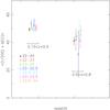Fig. B.1 Weighted mean of the lensing signal times the radius for a low-z and high-z LRG lens sample, measured with different source samples as indicated in the plot. For both lens samples, we find consistent results, suggesting that our measurement pipeline is robust and does not introduce a redshift-dependent bias.

Since this work aims at measuring the redshift dependence of the lensing signal, we have to be particularly careful with systematic effects that mimic a redshift scaling. One problem that requires attention is computing the mean lensing efficiency. For example, if we miss the high-redshift tail of the source redshift distribution, the mean lensing efficiency would be biased increasingly low for higher lens redshifts, which would mimic a redshift dependence in the lensing signal. Motivated by the differences in mean lensing efficiency computed from the photometric redshift catalogue from Ilbert et al. (2009) and Ilbert et al. (2013) at high lens redshifts, we performed the following test.

We divided our source sample into six different samples, with magnitude cuts of 22 <m_r′< 23, 23 <m_r′< 24, and 22 <m_r′< 22.5, 22.5 <m_r′< 23, 23 <m_r′< 23.5, 23.5 <m_r′< 24. We split the LRGs into a low-redshift sample with 0.15 <z< 0.5 and a high-redshift sample with 0.5 <z< 0.8 and measured their lensing signals using each source sample. Note that for each source sample, we separately determined the shear signal around random points, the mean lensing efficiencies using the Ilbert et al. (2013) photometric redshift catalogues, the contamination of source galaxies around the lenses, and the noise bias correction. We measured the weighted mean of the lensing signal times the projected separation, as that is roughly a constant with radius, over the range $\mathrm{0.15}\mathit{<}\mathit{r}\mathit{<}\mathrm{10}{\mathit{h}}_{\mathrm{70}}^{-1}$ Mpc. We show these values for the two LRG samples in Fig. B.1.

The weighted mean of the lensing signal of each lens sample is consistent for the various source samples. Clearly, the measurements are correlated for the source samples that overlap in apparent magnitude, but the four bins of 0.5 mag width are more or less independent (not completely, because they are similarly affected by cosmic variance). This result strongly suggests that the measurement process is robust.

We have repeated this test using the photometric redshift catalogue of Ilbert et al. (2009) instead. For the 0.15 <z< 0.5 LRG sample the results are consistent, but for the high-z sample, some bins differ by 2–3σ. This indicates a problem with the source redshift distribution used to compute the lensing efficiencies. Since the photometric redshift catalogue of Ilbert et al. (2013) gives consistent results for the different source samples, even at high redshifts, this suggests that the source redshift distribution is sufficiently accurately determined with the latter, but not with the former (see also the discussion in Hoekstra et al. 2015).

Appendix C: Fitting methodology

We used Bayesian inference techniques to determine the posterior probability distribution of the model parameters λ, given the data . According to Bayes’ theorem, 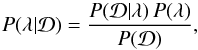$\mathit{P}\mathrm{\left(}\mathit{\lambda }\mathrm{\right|}\mathrm{𝒟}\mathrm{)}\mathrm{=}\frac{\mathit{P}\mathrm{\left(}\mathrm{𝒟}\mathrm{\right|}\mathit{\lambda }\mathrm{)}\hspace{0.17em}\mathit{P}\mathrm{(}\mathit{\lambda }\mathrm{)}}{\mathit{P}\mathrm{\left(}\mathrm{𝒟}\mathrm{\right)}}\mathit{,}$(C.1)where P(D | λ) is the likelihood of the data given the model parameters, P(λ) is the prior probability of these parameters, and $\mathit{P}\mathrm{\left(}\mathrm{𝒟}\mathrm{\right)}\mathrm{=}\mathrm{\int }\mathit{P}\mathrm{\left(}\mathrm{𝒟}\mathrm{\right|}\mathit{\lambda }\mathrm{)}\hspace{0.17em}\mathit{P}\mathrm{(}\mathit{\lambda }\mathrm{)}\hspace{0.17em}\mathrm{d}\mathit{\lambda }$(C.2)is called the evidence. Since we do not intend to perform model selection, the evidence just acts as a normalisation constant that does not need to be calculated. Therefore, the posterior distribution P(λ | D) is given by $\mathit{P}\mathrm{\left(}\mathit{\lambda }\mathrm{\right|}\mathrm{𝒟}\mathrm{)}\mathrm{\propto }\exp \left[\frac{\mathrm{-}{\mathit{\chi }}^{\mathrm{2}}\mathrm{\left(}\mathit{\lambda }\mathrm{\right)}}{\mathrm{2}}\right]\mathit{,}$(C.3)where ${\mathit{\chi }}^{\mathrm{2}}\mathrm{\left(}\mathit{\lambda }\mathrm{\right)}\mathrm{=}{\mathit{\chi }}_{\mathrm{ESD}}^{\mathrm{2}}\mathrm{=}\sum _{\mathit{k}\mathrm{=}\mathrm{1}}^{{\mathit{N}}_{\mathrm{lum}}}\sum _{\mathit{j}\mathrm{=}\mathrm{1}}^{{\mathit{N}}_{\mathrm{\Delta \Sigma }}}{\left[\frac{\mathrm{\Delta \Sigma }\mathrm{\left(}{\mathit{R}}_{\mathit{j}}\mathrm{\right|}{\mathit{L}}_{\mathit{k}}\mathrm{)}\mathrm{-}\begin{array}{c}\mathrm{􏽦}\\ \mathrm{\Delta \Sigma }\end{array}\mathrm{(}{\mathit{R}}_{\mathit{j}}\mathrm{\left|}{\mathit{L}}_{\mathit{k}}\mathrm{\right)}}{{\mathit{\sigma }}_{\mathrm{\Delta \Sigma }}\mathrm{\left(}{\mathit{R}}_{\mathit{j}}\mathrm{\right|}{\mathit{L}}_{\mathit{k}}\mathrm{)}}\right]}^{\mathrm{2}}\mathrm{·}$(C.4)$\begin{array}{c}{\mathrm{􏽦}}_{}\\ \mathrm{\Delta \Sigma }\end{array}$ denotes the model prediction, σ_ΔΣ is the corresponding error, N_lum = 3 and N_ΔΣ = 12,12,12,11 for the low- and high-redshift bins of the LOWZ and CMASS samples, respectively. For our fiducial model, the set of model parameters is λ_fid = (M_mean,σ_log M,f_conc), where

• M_mean is the mean halo mass for the k-th luminosity bin;

• σ_log M is the scatter of ⟨ N_c | M ⟩;

• f_conc is the normalisation of the c(M) relation.

When exploring model variations (see Sect. 4.1), we employed λ_miscen = (λ_fid,p_off,R_off) and λ_satfrac = (λ_fid,M₁). For all model parameters, we adopted a flat, sufficiently wide prior such that the results are not biased.

We sampled the posterior distribution of our model parameters given the data using a Markov chain Monte Carlo (MCMC). In particular, we implemented the Metropolis-Hastings algorithm to construct the MCMC. At any point in the chain, a trial model is generated using a method specified below. The χ² statistic for the trial model, ${\mathit{\chi }}_{\mathrm{try}}^{\mathrm{2}}$, is calculated using Eq. (C.4). This trial model is accepted to be a member of the chain with a probability given by ${\mathit{P}}_{\mathrm{accept}}\mathrm{=}\{\begin{array}{c}\\ \mathrm{1.0}& \mathrm{if} {\mathit{\chi }}_{\mathrm{try}}^{\mathrm{2}}\mathrm{\le }{\mathit{\chi }}_{\mathrm{cur}}^{\mathrm{2}}\\ \exp \mathrm{[}\mathrm{-}\mathrm{(}{\mathit{\chi }}_{\mathrm{try}}^{\mathrm{2}}\mathrm{-}{{\mathit{\chi }}_{\mathrm{cur}}^{\mathrm{2}}}^{\mathrm{)}}\mathit{/}{\mathrm{2}}^{\mathrm{]}}& \mathrm{if} {\mathit{\chi }}_{\mathrm{try}}^{\mathrm{2}}\mathit{>}{\mathit{\chi }}_{\mathrm{cur}}^{\mathrm{2}}\end{array}\mathit{,}$(C.5)where ${\mathit{\chi }}_{\mathrm{cur}}^{\mathrm{2}}$ denotes the χ² for the current model in the chain. We initialized the chain from a random position in our multi-dimensional parameter space and obtained a chain of ~500 000 models. We discarded the first 10 000 models (the burn-in period) allowing the chain to sample from a more probable part of the distribution. We used this chain of models to estimate the confidence levels on the parameters and on the lensing signal, as shown in Fig. 4.

A proper choice of the proposal distribution is very important to achieve fast convergence and a reasonable acceptance rate for the trial models. The posterior distribution in a multi-dimensional parameter space, such as the one we are dealing with, will have degeneracies and in general can be very difficult to sample from. We have adopted the following strategy to overcome these difficulties. During the first half of the burn-in stage, we chose an independent Gaussian proposal distribution for every model parameter, as is common for the Metropolis-Hastings

algorithm. Half-way through the burn-in stage, we performed a Fisher information matrix analysis at the best-fit model found thus far. The Fisher information matrix, given by ${\mathit{F}}_{\mathit{ij}}\mathrm{=}\mathrm{-}\frac{{\mathit{\partial }}^{\mathrm{2}}\ln \mathrm{ℒ}}{\mathit{\partial }{\mathit{\lambda }}_{\mathit{i}}\mathit{\partial }{\mathit{\lambda }}_{\mathit{j}}}\mathit{,}$(C.6)is an N_p × N_p symmetric matrix, where N_p denotes the number of parameters in our model, and ℒ ∝ e^{− χ2/ 2} is the likelihood. The inverse of the Fisher matrix gives the covariance matrix, C, of the posterior constraints on the model parameters. More importantly, the eigenvectors of the covariance matrix are an excellent guide to the degeneracies in the posterior distribution, and the corresponding eigenvalues set a scale for how wide the posterior ought to be in a given direction. Therefore, for the second half of the burn-in period, we used this information and a proposal distribution that is a multi-variate Gaussian centred on the current value of the parameters and with a covariance given by the aforementioned matrix. In practice, the trial model (λ_try) can be generated from the current model (λ_cur) using ${\mathit{\lambda }}_{\mathrm{try}}\mathrm{=}{\mathit{\lambda }}_{\mathrm{cur}}\mathrm{+}\mathit{\zeta }\hspace{0.17em}{A}{x}\mathit{,}$(C.7)where x is a vector consisting of N_p standard normal deviates, the matrix A is such that AA^T = C, and ζ is a parameter that we have chosen to achieve an average acceptance rate of ~30%. We repeated the Fisher matrix analysis at the end of the burn-in period (using the best-fit model found thus far) and used the covariance matrix to define our proposal distribution to be used for the MCMC. This strategy has proven to be extremely efficient in sampling posterior distributions for similar studies (see e.g. Cacciato et al. 2013, 2014).

Appendix D: k-corrected-only results

We have attempted to account for the evolution of the luminosities of LRGs by applying a luminosity evolution correction. Unfortunately, this correction is uncertain and will also add scatter to the corrected luminosities because LRGs cover a range of intrinsic properties such as formation age and metallicity, which complicates the interpretation of the results. Therefore, it is also interesting to apply only the k-correction to the absolute magnitudes. The resulting luminosities are closer to the real luminosities, meaning they have smaller scatter. Interpreting any trend in the luminosity-to-halo mass relation will be harder as both the luminosity and the halo mass may evolve simultaneously, but a comparison with simulations, for example, should be more straightforward.

Hence we divided the lens sample into bins of k-corrected absolute magnitude and redshift. Details of the lens samples can be found in Table D.1. The selection is also illustrated in Fig. 3. For each subsample, we stacked the lensing signal of all the lenses inside that bin and show the result in Fig. D.1. We fitted the halo model using the same set-up as before and show the best-fit models, together with the model uncertainties, in Fig. D.1. The corresponding effective masses and normalisations of the mass-concentration relation are listed in Table D.1.

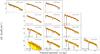Fig. D.1 Lensing signal ΔΣ of LOWZ (top two rows) and CMASS (bottom two rows) lenses as a function of projected separation for the five luminosity bins (after the k-correction is applied). The solid red lines show the best-fit halo model, the orange and yellow regions the 1 and 2σ model uncertainty, respectively. We fit the signal on scales between 0.05 and 2 ${\mathit{h}}_{\mathrm{70}}^{-1}$ Mpc.

Acknowledgments

We would like to thank Alexie Leauthaud and Claudia Maraston for useful discussions and suggestions. This work was supported by a grant from the German Space Agency DLR. H.H., M.C. and R.H. acknowledge support from NWO VIDI grant number 639.042.814 and ERC FP7 grant 279396. This work is based on observations obtained with MegaPrime/MegaCam, a joint project of CFHT and CEA/DAPNIA, at the Canada-France-Hawaii Telescope (CFHT) which is operated by the National Research Council (NRC) of Canada, the Institute National des Sciences de l’Univers of the Centre National de la Recherche Scientifique of France, and the University of Hawaii. We used the facilities of the Canadian Astronomy Data Centre operated by the NRC with the support of the Canadian Space Agency. Funding for SDSS-III has been provided by the Alfred P. Sloan Foundation, the Participating Institutions, the National Science Foundation, and the US Department of Energy Office of Science. The SDSS-III web site is http://www.sdss3.org/. SDSS-III is managed by the Astrophysical Research Consortium for the Participating Institutions of the SDSS-III Collaboration including the University of Arizona, the Brazilian Participation Group, Brookhaven National Laboratory, University of Cambridge, Carnegie Mellon University, University of Florida, the French Participation Group, the German Participation Group, Harvard University, the Instituto de Astrofisica de Canarias, the Michigan State/Notre Dame/JINA Participation Group, Johns Hopkins University, Lawrence Berkeley National Laboratory, Max Planck Institute for Astrophysics, Max Planck Institute for Extraterrestrial Physics, New Mexico State University, New York University, Ohio State University, Pennsylvania State University, University of Portsmouth, Princeton University, the Spanish Participation Group, University of Tokyo, University of Utah, Vanderbilt University, University of Virginia, University of Washington, and Yale University.

References

All Tables

All Figures

	Fig. 1 SDSS g − r and r − i colours versus redshift for the LRG sample used in this work. The solid cyan line indicates the median. The other lines show a range of Bruzual & Charlot (2003) SSP models, for various formation times (different colours) and metallicities (different line-styles) as indicated in the top-left of the figure.
In the text

Fig. 2 Top panel: k-correction as a function of redshift. The gray scale shows the k-corrections from the KCORRECT code, the solid cyan line indicates the median and the other coloured lines show the k-correction as predicted by a range of Bruzual & Charlot (2003) SSP models, for various formation times (different colours) and metallicities (different line-styles) as indicated in the top-left of the figure. Bottom panel: luminosity evolution correction as a function of redshift. For clarity, we only show a few of the Bruzual & Charlot (2003) model predictions. The thick green dot-dot-dashed line shows the correction we have used in this work, which is based on the Z = 0.02 instantaneous-burst model that formed 11 Gyr ago.

In the text

Fig. 3 Distribution of absolute magnitudes and redshifts of our LRG lenses after the k-correction (top) and after the k-correction and luminosity evolution correction (bottom). The solid cyan line indicates the median. The green dashed boxes show the redshift and luminosity cuts on our lens sample; the magenta pentagons indicate the mean redshift and luminosity of those bins. The total density of LRGs as a function of redshift is shown by the black and red histograms on the horizontal axis for the LOWZ and CMASS galaxies, respectively.

In the text

Fig. 4 Lensing signal ΔΣ of LOWZ (top two rows) and CMASS (bottom two rows) lenses as a function of projected separation for the three luminosity bins (after the (k + e)-correction is applied). The solid red lines show the best-fit halo model, the orange and yellow regions the 1 and 2σ model uncertainty, respectively. We fit the signal on scales between 0.05 and 2 ${\mathit{h}}_{\mathrm{70}}^{-1}$ Mpc.

In the text

	Fig. 5 Mean (k + e)-corrected luminosity versus the best-fit halo mass of the twelve lens samples. The different symbols indicate the different redshifts bins, as indicated in the figure. The coloured areas indicate the 68% confidence intervals of the power-law fits.
In the text

	Fig. 6 68% confidence contours for two parameters of the power-law fit between luminosity and halo mass.
In the text

	Fig. 7 Evolution of the amplitude of the power-law fit between luminosity and halo mass with redshift. The black dashed lines shows the predicted trend from pseudo-evolution (Diemer et al. 2013) for halo masses that are typical for LRGs, scaled to overlap with our first data point.
In the text

Fig. 8 Best-fit mass-concentration relation derived for the 0.15<z<0.29 LOWZ bin. The solid black line indicates the best-fit result and the turquoise area the 68% confidence intervals. The blue dotted line shows the reference relation from Duffy et al. (2008), whose amplitude we fit in the halo model. The red and green dotted-dashed lines show the relations from Macciò et al. (2008) and Dutton & Macciò (2014), respectively. The black points and the grey area are the results from direct fits to lensing data from Mandelbaum et al. (2008).

In the text

	Fig. 9 Best-fit normalisation of the mass-concentration relation from Duffy et al. (2008) for the four redshift slices. Filled symbols show the results for the nominal run, open symbols for the miscentring run. The open symbols have been shifted to the right for clarity.
In the text

	Fig. B.1 Weighted mean of the lensing signal times the radius for a low-z and high-z LRG lens sample, measured with different source samples as indicated in the plot. For both lens samples, we find consistent results, suggesting that our measurement pipeline is robust and does not introduce a redshift-dependent bias.
In the text

Fig. D.1 Lensing signal ΔΣ of LOWZ (top two rows) and CMASS (bottom two rows) lenses as a function of projected separation for the five luminosity bins (after the k-correction is applied). The solid red lines show the best-fit halo model, the orange and yellow regions the 1 and 2σ model uncertainty, respectively. We fit the signal on scales between 0.05 and 2 ${\mathit{h}}_{\mathrm{70}}^{-1}$ Mpc.

In the text

References

- Ahn, C. P., Alexandroff, R., Allen de Prieto, C., et al. 2012, ApJS, 203, 21 [NASA ADS] [CrossRef] [Google Scholar]
- Ahn, C. P., Alexandroff, R., Allen de Prieto, C., et al. 2014, ApJS, 211, 17 [NASA ADS] [CrossRef] [Google Scholar]
- Banerji, M., Ferreras, I., Abdalla, F. B., Hewett, P., & Lahav, O. 2010, MNRAS, 402, 2264 [NASA ADS] [CrossRef] [Google Scholar]
- Baugh, C. M. 2006, Rep. Prog. Phys., 69, 3101 [NASA ADS] [CrossRef] [Google Scholar]
- Bédorf, J., & Portegies Zwart, S. 2013, MNRAS, 431, 767 [NASA ADS] [CrossRef] [Google Scholar]
- Blake, C., Collister, A., & Lahav, O. 2008, MNRAS, 385, 1257 [NASA ADS] [CrossRef] [Google Scholar]
- Blanton, M. R., & Roweis, S. 2007, AJ, 133, 734 [NASA ADS] [CrossRef] [Google Scholar]
- Blanton, M. R., Brinkmann, J., Csabai, I., et al. 2003, AJ, 125, 2348 [NASA ADS] [CrossRef] [Google Scholar]
- Brimioulle, F., Seitz, S., Lerchster, M., Bender, R., & Snigula, J. 2013, MNRAS, 432, 1046 [NASA ADS] [CrossRef] [Google Scholar]
- Bruzual, G., & Charlot, S. 2003, MNRAS, 344, 1000 [NASA ADS] [CrossRef] [Google Scholar]
- Cacciato, M., van den Bosch, F. C., More, S., et al. 2009, MNRAS, 394, 929 [NASA ADS] [CrossRef] [Google Scholar]
- Cacciato, M., van den Bosch, F. C., More, S., Mo, H., & Yang, X. 2013, MNRAS, 430, 767 [NASA ADS] [CrossRef] [Google Scholar]
- Cacciato, M., van Uitert, E., & Hoekstra, H. 2014, MNRAS, 437, 377 [NASA ADS] [CrossRef] [Google Scholar]
- Cannon, R., Drinkwater, M., Edge, A., et al. 2006, MNRAS, 372, 425 [NASA ADS] [CrossRef] [Google Scholar]
- Carson, D. P., & Nichol, R. C. 2010, MNRAS, 408, 213 [NASA ADS] [CrossRef] [Google Scholar]
- Chabrier, G. 2003, PASP, 115, 763 [NASA ADS] [CrossRef] [Google Scholar]
- Choi, A., Tyson, J. A., Morrison, C. B., et al. 2012, ApJ, 759, 101 [NASA ADS] [CrossRef] [Google Scholar]
- Cimatti, A., Daddi, E., & Renzini, A. 2006, A&A, 453, L29 [NASA ADS] [CrossRef] [EDP Sciences] [Google Scholar]
- Conroy, C., Gunn, J. E., & White, M. 2009, ApJ, 699, 486 [NASA ADS] [CrossRef] [Google Scholar]
- Conroy, C., White, M., & Gunn, J. E. 2010, ApJ, 708, 58 [NASA ADS] [CrossRef] [Google Scholar]
- Cool, R. J., Eisenstein, D. J., Fan, X., et al. 2008, ApJ, 682, 919 [NASA ADS] [CrossRef] [Google Scholar]
- Cooray, A., & Sheth, R. 2002, Phys. Rep., 372, 1 [NASA ADS] [CrossRef] [Google Scholar]
- Dawson, K. S., Schlegel, D. J., Ahn, C. P., et al. 2013, AJ, 145, 10 [Google Scholar]
- Diemer, B., More, S., & Kravtsov, A. V. 2013, ApJ, 766, 25 [NASA ADS] [CrossRef] [Google Scholar]
- Driver, S. P., Norberg, P., Baldry, I. K., et al. 2009, Astron. Geophys., 50, 050000 [Google Scholar]
- Driver, S. P., Hill, D. T., Kelvin, L. S., et al. 2011, MNRAS, 413, 971 [NASA ADS] [CrossRef] [Google Scholar]
- Duffy, A. R., Schaye, J., Kay, S. T., & Dal la Vecchia, C. 2008, MNRAS, 390, L64 [NASA ADS] [CrossRef] [Google Scholar]
- Duffy, A. R., Schaye, J., Kay, S. T., et al. 2010, MNRAS, 405, 2161 [NASA ADS] [Google Scholar]
- Dutton, A. A., & Macciò, A. V. 2014, MNRAS, 441, 3359 [NASA ADS] [CrossRef] [Google Scholar]
- Eisenstein, D. J., Annis, J., Gunn, J. E., et al. 2001, AJ, 122, 2267 [NASA ADS] [CrossRef] [Google Scholar]
- Fakhouri, O., & Ma, C.-P. 2010, MNRAS, 401, 2245 [NASA ADS] [CrossRef] [Google Scholar]
- Fakhouri, O., Ma, C.-P., & Boylan-Kolchin, M. 2010, MNRAS, 406, 2267 [NASA ADS] [CrossRef] [Google Scholar]
- Gabor, J. M., & Davé, R. 2012, MNRAS, 427, 1816 [NASA ADS] [CrossRef] [Google Scholar]
- Gilbank, D. G., Gladders, M. D., Yee, H. K. C., & Hsieh, B. C. 2011, AJ, 141, 94 [NASA ADS] [CrossRef] [Google Scholar]
- Glazebrook, K., Abraham, R. G., McCarthy, P. J., et al. 2004, Nature, 430, 181 [NASA ADS] [CrossRef] [Google Scholar]
- Greisel, N., Seitz, S., Drory, N., et al. 2013, ApJ, 768, 117 [NASA ADS] [CrossRef] [Google Scholar]
- Guo, Q., White, S., Boylan-Kolchin, M., et al. 2011, MNRAS, 413, 101 [NASA ADS] [CrossRef] [Google Scholar]
- Guo, H., Zheng, Z., Zehavi, I., et al. 2014, MNRAS, 441, 2398 [NASA ADS] [CrossRef] [Google Scholar]
- Heymans, C., Van Waerbeke, L., Miller, L., et al. 2012, MNRAS, 427, 146 [NASA ADS] [CrossRef] [Google Scholar]
- Hinshaw, G., Weiland, J. L., Hill, R. S., et al. 2009, ApJS, 180, 225 [NASA ADS] [CrossRef] [Google Scholar]
- Hoekstra, H., Franx, M., Kuijken, K., & Squires, G. 1998, ApJ, 504, 636 [NASA ADS] [CrossRef] [Google Scholar]
- Hoekstra, H., Franx, M., & Kuijken, K. 2000, ApJ, 532, 88 [NASA ADS] [CrossRef] [Google Scholar]
- Hoekstra, H., Hsieh, B. C., Yee, H. K. C., Lin, H., & Gladders, M. D. 2005, ApJ, 635, 73 [NASA ADS] [CrossRef] [Google Scholar]
- Hoekstra, H., Herbonnet, R., Muzzin, A., et al. 2015, MNRAS, 449, 685 [NASA ADS] [CrossRef] [Google Scholar]
- Hudson, M. J., Gillis, B. R., Coupon, J., et al. 2015, MNRAS, 447, 298 [NASA ADS] [CrossRef] [Google Scholar]
- Ilbert, O., Capak, P., Salvato, M., et al. 2009, ApJ, 690, 1236 [NASA ADS] [CrossRef] [Google Scholar]
- Ilbert, O., McCracken, H. J., Le Fèvre, O., et al. 2013, A&A, 556, A55 [NASA ADS] [CrossRef] [EDP Sciences] [Google Scholar]
- Kacprzak, T., Zuntz, J., Rowe, B., et al. 2012, MNRAS, 427, 2711 [NASA ADS] [CrossRef] [Google Scholar]
- Kaiser, N., Squires, G., & Broadhurst, T. 1995, ApJ, 449, 460 [NASA ADS] [CrossRef] [Google Scholar]
- Kaviraj, S., Schawinski, K., Devriendt, J. E. G., et al. 2007, ApJS, 173, 619 [NASA ADS] [CrossRef] [Google Scholar]
- Kaviraj, S., Tan, K.-M., Ellis, R. S., & Silk, J. 2011, MNRAS, 411, 2148 [NASA ADS] [CrossRef] [Google Scholar]
- Komatsu, E., Smith, K. M., Dunkley, J., et al. 2011, ApJS, 192, 18 [NASA ADS] [CrossRef] [Google Scholar]
- Laureijs, R., Amiaux, J., Arduini, S., et al. 2011, ArXiv e-prints [arXiv:1110.3193] [Google Scholar]
- Leauthaud, A., Tinker, J., Bundy, K., et al. 2012, ApJ, 744, 159 [NASA ADS] [CrossRef] [Google Scholar]
- Leauthaud, A.J., Benson, A., Civano, F., et al. 2015, MNRAS, 446, 1874 [NASA ADS] [CrossRef] [Google Scholar]
- Li, R., Mo, H. J., Fan, Z., et al. 2009, MNRAS, 394, 1016 [NASA ADS] [CrossRef] [Google Scholar]
- Liu, G., Lu, Y., Chen, X., et al. 2012, ApJ, 758, 107 [NASA ADS] [CrossRef] [Google Scholar]
- López-Sanjuan, C., Le Fèvre, O., Ilbert, O., et al. 2012, A&A, 548, A7 [NASA ADS] [CrossRef] [EDP Sciences] [Google Scholar]
- Luppino, G. A., & Kaiser, N. 1997, ApJ, 475, 20 [NASA ADS] [CrossRef] [Google Scholar]
- Macciò, A. V., Dutton, A. A., van den Bosch, F. C., et al. 2007, MNRAS, 378, 55 [NASA ADS] [CrossRef] [Google Scholar]
- Macciò, A. V., Dutton, A. A., & van den Bosch, F. C. 2008, MNRAS, 391, 1940 [NASA ADS] [CrossRef] [Google Scholar]
- Mandelbaum, R., Seljak, U., Cool, R. J., et al. 2006a, MNRAS, 372, 758 [NASA ADS] [CrossRef] [Google Scholar]
- Mandelbaum, R., Seljak, U., Kauffmann, G., Hirata, C. M., & Brinkmann, J. 2006b, MNRAS, 368, 715 [Google Scholar]
- Mandelbaum, R., Seljak, U., & Hirata, C. M. 2008, J. Cosmol. Astropart. Phys., 8, 6 [Google Scholar]
- Mandelbaum, R., Slosar, A., Baldauf, T., et al. 2013, MNRAS, 432, 1544 [NASA ADS] [CrossRef] [Google Scholar]
- Maraston, C., Strömbäck, G., Thomas, D., Wake, D. A., & Nichol, R. C. 2009, MNRAS, 394, L107 [NASA ADS] [CrossRef] [Google Scholar]
- Masaki, S., Hikage, C., Takada, M., Spergel, D. N., & Sugiyama, N. 2013, MNRAS, 433, 3506 [NASA ADS] [CrossRef] [Google Scholar]
- Melchior, P., & Viola, M. 2012, MNRAS, 424, 2757 [NASA ADS] [CrossRef] [Google Scholar]
- Miyatake, H., More, S., Mandelbaum, R., et al. 2015, ApJ, 806, 1 [NASA ADS] [CrossRef] [Google Scholar]
- More, S., van den Bosch, F. C., & Cacciato, M. 2009, MNRAS, 392, 917 [NASA ADS] [CrossRef] [Google Scholar]
- More, S., Miyatake, H., Mandelbaum, R., et al. 2015, ApJ, 806, 2 [NASA ADS] [CrossRef] [Google Scholar]
- Navarro, J. F., Frenk, C. S., & White, S. D. M. 1996, ApJ, 462, 563 [NASA ADS] [CrossRef] [Google Scholar]
- Nikoloudakis, N., Shanks, T., & Sawangwit, U. 2013, MNRAS, 429, 2032 [NASA ADS] [CrossRef] [Google Scholar]
- Parejko, J. K., Sunayama, T., Padmanabhan, N., et al. 2013, MNRAS, 429, 98 [NASA ADS] [CrossRef] [Google Scholar]
- Pickles, A. J. 1998, PASP, 110, 863 [CrossRef] [Google Scholar]
- Planck Collaboration XVI. 2014, A&A, 571, A16 [NASA ADS] [CrossRef] [EDP Sciences] [Google Scholar]
- Pozzetti, L., Bolzonella, M., Zucca, E., et al. 2010, A&A, 523, A13 [NASA ADS] [CrossRef] [EDP Sciences] [Google Scholar]
- Refregier, A., Kacprzak, T., Amara, A., Bridle, S., & Rowe, B. 2012, MNRAS, 425, 1951 [NASA ADS] [CrossRef] [Google Scholar]
- Robotham, A. S. G., Norberg, P., Driver, S. P., et al. 2011, MNRAS, 416, 2640 [NASA ADS] [CrossRef] [Google Scholar]
- Roseboom, I. G., Pimbblet, K. A., Drinkwater, M. J., et al. 2006, MNRAS, 373, 349 [NASA ADS] [CrossRef] [Google Scholar]
- Rowe, B., Jarvis, M., Mandelbaum, R., et al. 2014, Astron. Comput., 10, 121 [Google Scholar]
- Ruiz, P., Trujillo, I., & Mármol-Queraltó, E. 2014, MNRAS, 442, 347 [NASA ADS] [CrossRef] [Google Scholar]
- Salim, S., & Rich, R. M. 2010, ApJ, 714, L290 [NASA ADS] [CrossRef] [Google Scholar]
- Sawangwit, U., Shanks, T., Abdalla, F. B., et al. 2011, MNRAS, 416, 3033 [NASA ADS] [CrossRef] [Google Scholar]
- Scarlata, C., Carollo, C. M., Lilly, S. J., et al. 2007, ApJS, 172, 494 [NASA ADS] [CrossRef] [Google Scholar]
- Schawinski, K., Kaviraj, S., Khochfar, S., et al. 2007, ApJS, 173, 512 [NASA ADS] [CrossRef] [Google Scholar]
- Schaye, J., Crain, R. A., Bower, R. G., et al. 2015, MNRAS, 446, 521 [Google Scholar]
- Schlegel, D. J., Finkbeiner, D. P., & Davis, M. 1998, ApJ, 500, 525 [NASA ADS] [CrossRef] [Google Scholar]
- Seljak, U. 2000, MNRAS, 318, 203 [NASA ADS] [CrossRef] [Google Scholar]
- Semboloni, E., Hoekstra, H., Schaye, J., van Daalen, M. P., & McCarthy, I. G. 2011, MNRAS, 417, 2020 [NASA ADS] [CrossRef] [Google Scholar]
- Simet, M., & Mandelbaum, R. 2014, MNRAS, 449, 1259 [Google Scholar]
- Skibba, R. A., van den Bosch, F. C., Yang, X., et al. 2011, MNRAS, 410, 417 [NASA ADS] [CrossRef] [Google Scholar]
- Tal, T., Wake, D. A., van Dokkum, P. G., et al. 2012, ApJ, 746, 138 [NASA ADS] [CrossRef] [Google Scholar]
- Thomas, D., Steele, O., Maraston, C., et al. 2013, MNRAS, 431, 1383 [NASA ADS] [CrossRef] [Google Scholar]
- Tinker, J. L., Robertson, B. E., Kravtsov, A. V., et al. 2010, ApJ, 724, 878 [NASA ADS] [CrossRef] [Google Scholar]
- Tinker, J. L., Leauthaud, A., Bundy, K., et al. 2013, ApJ, 778, 93 [NASA ADS] [CrossRef] [Google Scholar]
- Tojeiro, R., & Percival, W. J. 2010, MNRAS, 405, 2534 [NASA ADS] [Google Scholar]
- Tojeiro, R., & Percival, W. J. 2011, MNRAS, 417, 1114 [NASA ADS] [CrossRef] [Google Scholar]
- Tojeiro, R., Percival, W. J., Heavens, A. F., & Jimenez, R. 2011, MNRAS, 413, 434 [NASA ADS] [CrossRef] [Google Scholar]
- Tojeiro, R., Percival, W. J., Wake, D. A., et al. 2012, MNRAS, 424, 136 [NASA ADS] [CrossRef] [Google Scholar]
- van Daalen, M. P., Schaye, J., Booth, C. M., & Dal la Vecchia, C. 2011, MNRAS, 415, 3649 [NASA ADS] [CrossRef] [Google Scholar]
- van den Bosch, F. C., More, S., Cacciato, M., Mo, H., & Yang, X. 2013, MNRAS, 430, 725 [NASA ADS] [CrossRef] [Google Scholar]
- van Uitert, E., Hoekstra, H., Velander, M., et al. 2011, A&A, 534, A14 [NASA ADS] [CrossRef] [EDP Sciences] [Google Scholar]
- van Uitert, E., Hoekstra, H., Franx, M., et al. 2013, A&A, 549, A7 [NASA ADS] [CrossRef] [EDP Sciences] [Google Scholar]
- Velander, M., van Uitert, E., Hoekstra, H., et al. 2014, MNRAS, 437, 2111 [NASA ADS] [CrossRef] [Google Scholar]
- Velliscig, M., van Daalen, M. P., Schaye, J., et al. 2014, MNRAS, 442, 2641 [NASA ADS] [CrossRef] [Google Scholar]
- Vogelsberger, M., Genel, S., Springel, V., et al. 2014, MNRAS, 444, 1518 [NASA ADS] [CrossRef] [Google Scholar]
- Wake, D. A., Nichol, R. C., Eisenstein, D. J., et al. 2006, MNRAS, 372, 537 [NASA ADS] [CrossRef] [Google Scholar]
- Wake, D. A., Sheth, R. K., Nichol, R. C., et al. 2008, MNRAS, 387, 1045 [NASA ADS] [CrossRef] [Google Scholar]
- Wetzel, A. R., & Nagai, D. 2014, ApJ, submitted [arXiv:1412.0662] [Google Scholar]
- White, S. D. M., & Rees, M. J. 1978, MNRAS, 183, 341 [NASA ADS] [CrossRef] [Google Scholar]
- White, M., Blanton, M., Bolton, A., et al. 2011, ApJ, 728, 126 [NASA ADS] [CrossRef] [Google Scholar]
- York, D. G., Adelman, J., Anderson, Jr., J. E., et al. 2000, AJ, 120, 1579 [Google Scholar]
- Zheng, Z., Zehavi, I., Eisenstein, D. J., Weinberg, D. H., & Jing, Y. P. 2009, ApJ, 707, 554 [NASA ADS] [CrossRef] [Google Scholar]
All Tables
Power-law parameters, normalisation of the mass-concentration relations, and reduced chi-squared values for various runs as described in the text.