| Issue |
A&A
Volume 579, July 2015
|
|
|---|---|---|
| Article Number | A102 | |
| Number of page(s) | 28 | |
| Section | Extragalactic astronomy | |
| DOI | https://doi.org/10.1051/0004-6361/201525712 | |
| Published online | 07 July 2015 | |
Hα imaging of the Herschel Reference Survey
The star formation properties of a volume-limited, K-band-selected sample of nearby late-type galaxies⋆,⋆⋆
1 Aix Marseille Université, CNRS, LAM (Laboratoire d’Astrophysique de Marseille) UMR 7326, 13388 Marseille, France
e-mail: This email address is being protected from spambots. You need JavaScript enabled to view it.
2 Universitäts-Sternwarte München, Schenierstrasse 1, 81679 München, Germany
3 Max-Planck-Institut für Extraterrestrische Physik, Giessenbachstrasse, 85748 Garching, Germany
e-mail: This email address is being protected from spambots. You need JavaScript enabled to view it.
4 Università di Milano-Bicocca, piazza della Scienza 3, 20100 Milano, Italy
e-mail: This email address is being protected from spambots. You need JavaScript enabled to view it.
5 University of Crete, Department of Physics, 71003 Heraklion, Greece
e-mail: This email address is being protected from spambots. You need JavaScript enabled to view it.
6 Institute for Astronomy, Astrophysics, Space Applications and Remote Sensing, National Observatory of Athens, 15236 Penteli, Greece
7 Sterrenkundig Observatorium, Universiteit Gent, Krijgslaan 281-S9, 9000 Gent, Belgium
e-mail: This email address is being protected from spambots. You need JavaScript enabled to view it.
Received: 21 January 2015
Accepted: 7 April 2015
Abstract
We present new Hα+[NII] imaging data of late-type galaxies in the Herschel Reference Survey aimed at studying the star formation properties of a K-band-selected, volume-limited sample of nearby galaxies. The Hα+[NII] data are corrected for [NII] contamination and dust attenuation using different recipes based on the Balmer decrement and the 24 μm luminosities. We show that the Hα luminosities derived with different corrections give consistent results only whenever the uncertainty on the estimate of the Balmer decrement is σ [C(Hβ)] ≤ 0.1. We used these data to derive the star formation rate of the late-type galaxies of the sample and compare these estimates to those determined using independent monochromatic tracers (far-UV, radio continuum) or the output of spectral energy distribution (SED) fitting codes. This comparison suggests that the 24 μm based dust extinction correction for the Hα data might not be universal and that it should be used with caution in all objects with a low star formation activity, where dust heating can be dominated by the old stellar population. Furthermore, because of the sudden truncation of the star formation activity of cluster galaxies occurring after their interaction with the surrounding environment, the stationarity conditions required to transform monochromatic fluxes into star formation rates might not always be satisfied in tracers other than the Hα luminosity. In a similar way, the parametrisation of the star formation history generally used in SED fitting codes might not be adequate for these recently interacting systems. We then use the derived star formation rates to study the star formation rate luminosity distribution and the typical scaling relations of the late-type galaxies of the HRS. We observe a systematic decrease of the specific star formation rate with increasing stellar mass, stellar mass surface density, and metallicity. We also observe an increase of the asymmetry and smoothness parameters measured in the Hα-band with increasing specific star formation rate, probably induced by an increase of the contribution of giant HII regions to the Hα luminosity function in star-forming low-luminosity galaxies.
Key words: galaxies: spiral / galaxies: star formation / galaxies: fundamental parameters / galaxies: clusters: general / galaxies: photometry / galaxies: luminosity function, mass function
Appendices are available in electronic form at http://www.aanda.org
Full Tables 1–4, 6–7, 10 are only available at the CDS via anonymous ftp to cdsarc.u-strasbg.fr (130.79.128.5) or via http://cdsarc.u-strasbg.fr/viz-bin/qcat?J/A+A/579/A102
© ESO, 2015
1. Introduction
Star formation is a key process in the study of galaxy evolution. Stars are formed within giant molecular clouds through the collapse of the gaseous component. Once formed, massive stars produce and inject metals into the interstellar medium that later aggregate to form dust (Valiante et al. 2009). The various ingredients of the interstellar medium, including those produced during stellar evolution, all contribute to regulating the matter cycle in galaxies. The formation of the molecular gas occurs primarily on dust grains (Hollenbach & Salpeter 1971; Wolfire et al. 2008). Dust also absorbs the interstellar radiation field and is thus an important parameter in the cooling process of the gas (Bakes & Tielens 1994; Wolfire et al. 1995; Hollenbach & Tielens 1997). Massive stars can also inject a large amount of kinetic energy into the interstellar medium, favouring the ionisation of the surrounding gas and the dissociation of the molecular component, but also cloud-cloud collisions important in the process of star formation.
The hydrogen recombination lines are due to the cascade of electrons captured by the hydrogen nucleus once photoionised by the far-UV (FUV) radiation (λ< 912 Å) in HII regions. This highly energetic UV radiation is mainly emitted by massive (mstar> 8 M⊙) O-B stars, whose life on the main sequence is very short (<107 yr). Their presence thus indicates recent episodes of star formation. The Hα Balmer line (λ 6563 Å) is the brightest of the hydrogen recombination lines. This line is easily accessible from ground-based facilities in local galaxies since it is located in the visible spectral domain. Under specific conditions, its emission is proportional to the number of newly formed stars and can thus be used as a direct tracer of star formation (Kennicutt et al. 1994; Kennicutt 1998; Boselli et al. 2001). Star formation rates are proportional to Hα luminosities if the star formation activity of the targets is constant on a timescale at least as long as the time that the ionising stars spend on the main sequence (~107 yr). Only under these conditions does the number of stars that leave the main sequence equal that of newly formed stars. The constant of proportionality between the Hα luminosity and the star formation rate depends on the initial mass function (IMF), on the metallicity, and on several assumptions in the photoionisation models, and can be estimated using population synthesis models.
Hα luminosities, however, can be converted into star formation rates only once they have been corrected for dust attenuation. This is generally done using the Balmer decrement (Lequeux et al. 1981), which is determined by comparing the observed Hα/Hβ flux ratio to the value expected for the typical conditions in HII regions (2.86, Case B; Osterbrock & Ferland 2006). Spectroscopic observations can be used for this purpose. An intermediate spectral resolution (R ~ 1000) is required to separate the emission of the Hα line from that of the two bracketing [NII] lines (λλ 6548, 6584 Å), while good signal-to-noise is needed to determine the underlying Balmer absorption produced by the stellar atmosphere of young stars. The accurate determination of the Balmer decrement is thus non-trivial, in particular in normal nearby galaxies characterised by a relatively low or moderate activity of star formation. Indeed, in these galaxies the intensity of the emission lines and, in particular, that of Hβ is relatively low and often comparable to the intensity of the underlying absorption. It is thus fundamental to understand to what limit in signal-to-noise the Balmer decrement can be accurately determined without introducing systematic errors in the estimate of the star formation rate (Groves et al. 2012). This is also crucial for quantifying the uncertainties on the determination of the dust attenuation of galaxies up to z ~ 1, which is often estimated using higher order Balmer lines (Hβ, λ4861 Å; Hγ, λ4340 Å; Hδ, λ4101Å). These lines are characterised by lower intensity and higher underlying absorption with respect to Hα (e.g. Momcheva et al. 2013). It is also critical to estimate whether the exclusion of objects with low Hβ emission from the analysis of the star formation properties of complete samples of galaxies biases the results. Galaxies with low Hβ emission are indeed objects with low star formation activity and/or high dust attenuation.
To overcome these technical difficulties, different tracers have been proposed in the literature either for correcting the observed Hα luminosities or for measuring star formation rates (e.g. Kennicutt 1998; Kennicutt et al. 2009; Hao et al. 2011; Kennicutt & Evans 2012). Using the same arguments as for the Hα line, any tracer of the young stellar population can be converted, under some assumptions, into star formation rates. The most widely used tracers are the dust-corrected FUV and the radio continuum luminosities. At 20 cm, the radio continuum emission of galaxies is mainly due to the synchrotron emission of relativistic electrons spinning in weak magnetic fields (e.g. Lequeux 1971; Condon 1992). These electrons are accelerated in supernovae remnants and are thus tightly related to the youngest stellar populations of galaxies. The FUV and radio continuum luminosities can be converted into star formation rates whenever the star formation activity of galaxies is constant over ~108 yrs, a timescale that is ten times longer than necessary when using the Hα luminosity, making these tracers more uncertain in objects suddenly changing their star formation activity with time. When multifrequency data are available, the star formation activity of galaxies can also be determined through fitting their spectral energy distribution (SED) with specific codes. The accuracy of this technique, which has the advantage of providing a consistent estimate of the contribution of dust attenuation to the stellar emission when UV, optical, and infrared data are available, depends on the sampling of the different photometric bands. It also depends on the chosen parametrisation of the star formation history of the galaxies, which is generally done with simple empirical relations. Compared to monochromatic tracers, this method has the advantage of accounting for possible variations in the star formation history of galaxies, even though these variations are not easily constrained (e.g. Buat et al. 2014).
The direct comparison of these different tracers is therefore crucial for identifying and quantifying their limits and uncertainties, as well as for understanding whether the use of a specific correction or calibration can introduce important systematic biases in the derived star formation rates (Kennicutt 1998; Kennicutt & Evans 2012; Kennicutt et al. 2009; Calzetti et al. 2007, 2010; Salim et al. 2007; Lee et al. 2009; Boselli et al. 2009). The comparison of these tracers must be carried out on well-defined samples of galaxies spanning the widest possible range in the parameter space and having the largest possible data coverage over all wavelengths (e.g. Buat et al. 2014).
Herschel Reference Survey.
The Herschel Reference Sample (Boselli et al. 2010) is ideal for this purpose. Composed of 323 nearby galaxies, this sample is volume-limited (15 ≤ distance ≤ 25 Mpc) and K-band-selected, which roughly corresponds to a stellar mass selection (Gavazzi et al. 1996). It also includes galaxies of all morphological types in the stellar mass range 5 × 10⁸ ≤ Mstar ≤ 1011 M⊙. The sample has been defined to study the physical properties of the interstellar medium, the star formation process, and the effects of the environment on galaxy evolution in normal galaxies. It thus includes galaxies in different density regions, from the sparse field to the rich core of the Virgo cluster. We have been collecting multifrequency data covering the entire electromagnetic spectrum, including UV GALEX and visible SDSS data (Boselli et al. 2011; Cortese et al. 2012), near- (2MASS), mid- and far-IR WISE (Ciesla et al. 2014), Spitzer (Bendo et al. 2012a; Ciesla et al. 2014), and Herschel (Ciesla et al. 2012; Cortese et al. 2014) data, while radio continuum data at 20 cm are available from the NVSS survey (Condon et al. 1998). Medium-resolution (R ~ 1000) integrated spectroscopic data are also available (Boselli et al. 2013), as well as HI and CO data (Boselli et al. 2014a). The purpose of this article is to use this unique sample and set of data to determine and compare different tracers of star formation, derived from both monochromatic luminosities and SED fitting techniques, in order to determine their range of validity, their strengths, and limits. We then use these data to trace the statistical properties of the star formation activity of the late-type galaxies of the sample, including their star formation rate distribution, scaling relations, and structural and morphological CAS parameters (Conselice 2003), for both normal and cluster galaxies. There are indeed strong indications that the star formation properties of cluster galaxies are strongly affected by the hostile environment in which they reside (e.g. Boselli & Gavazzi 2006, 2014).
The paper is structured as follows. In Sect. 2 we describe the sample, in Sect. 3 the observations, and in Sect. 4 the data reduction. The data are analysed in Sects. 5 and 6, and the conclusions summarised in Sect. 7. In three different appendices, we present the new spectroscopic data determined using the gandalf code, the radio continuum data at 20 cm taken from the literature and used in the analysis, and we list the recipes used to convert observed luminosities into star formation rates. We limit our analysis to the late-type galaxies of the sample (Sa-Im-BCD). It is indeed known that the Hα emission in early types (E-S0) does not necessarily come from the photoionisation of the gas by the young stellar populations (several of these early-type objects are also strong X-ray emitters). Furthermore, their FUV emission is generally due to very evolved stars (O’Connell 1999; Boselli et al. 2005) not associated to any event of star formation, while their radio continuum emission might be dominated by the contribution of the central AGN (M 87 and M 84 are well known powerful radio galaxies).
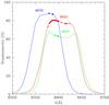 |
Fig. 1 Transmissivity of the ON-band (6603, 6607, 6570 Å) filters. Points indicate the throughput at the wavelength corresponding to the Hα line at the redshift of the target galaxies. |
2. The sample
The observed sample is composed of those HRS late-type galaxies without Hα imaging data available in the literature (see Table 1). It also includes a few objects with Hα+[NII] data from aperture photometry (Kennicutt & Kent 1983; Romanishin 1990). Combined with Hα+[NII] imaging data available in the literature, mostly gathered during our previous survey of the Virgo cluster (Boselli & Gavazzi 2002; Boselli et al. 2002; Gavazzi et al. 2002, 2006), the HRS sample is now complete at the 87% level and to 98% if limited to late-type galaxies. Because of the presence of bright stars close to the target, whose reflection causes unwanted extended low surface brightness structures on the images, six objects could not be observed. The HRS sample is listed in Table 1, arranged as follows:
-
Column 1: Herschel Reference Sample (HRS) name fromBoselli et al. (2010).
-
Column 2: Zwicky name, from the Catalogue of Galaxies and of Cluster of Galaxies (CGCG; Zwicky et al. 1961–1968).
-
Column 3: Virgo Cluster Catalogue (VCC) name from Binggeli et al. (1985).
-
Column 4: Uppsala General Catalog (UGC) name (Nilson 1973).
-
Column 5: New General Catalogue (NGC) name (Dreyer 1888).
-
Column 6: Index Catalogue (IC) name (Dreyer 1895).
-
Columns 7 and 8: J2000 right ascension and declination from NED.
-
Column 9: morphological type from NED or from our own classification if not available.
-
Column 10: distance, in Mpc. Distances have been determined from the recessional velocity assuming a Hubble constant H0 = 70 km s-1 Mpc-1 for galaxies outside the Virgo cluster, and assumed to be 17 Mpc for galaxies belonging to Virgo, with the exception of those located in the Virgo cluster B substructure (23 Mpc; Gavazzi et al. 1999).
-
Column 11: stellar mass from Cortese et al. (2012a), determined following the prescription of Zibetti et al. (2009) based on the i-band luminosity and g−i mass-to-light ratio. For galaxies without SDSS g and i-band data (11 objects, marked with a in Table 1), stellar masses have been computed using the prescription of Boselli et al. (2009) based on the H-band luminosity and B−H mass-to-light ratio.
-
Column 12: g-band optical isophotal diameter (24.5 mag arcsec-2) from Cortese et al. (2012a). For the HRS galaxies without SDSS images, the g-band isophotal diameter was determined from the relation r24.5(g) = 0.871(±0.017)r25(B) + 6.041(±2.101), where r25(B) is the radius given in NED (Boselli et al. 2014a).
-
Column 13: inclination of the galaxy, determined using the prescription based on the morphological type described in Haynes & Giovanelli (1984) and the i-band ellipticity given in Cortese et al. (2012a).
-
Column 14: Heliocentric radial velocity (in km s-1), from HI data when available (Boselli et al. 2014a), otherwise from NED.
-
Column 15: cluster or cloud membership from Gavazzi et al. (1999) for Virgo and Tully (1987) or Nolthenius (1993) whenever available, or from our own estimate (Boselli et al. 2010).
-
Column 16: code to indicate whether Hα+[NII] data are available (1) or not (0).
Hα observational parameters of the 138 target galaxies.
Hα+[NII] fluxes and equivalent widths.
3. Observations
The Hα+[NII] narrow band imaging of 138 HRS late-type galaxies has been obtained during different observing runs from 2006 to 2012 with the 2.1 m and the 1.5 m telescopes at San Pedro Martir (SPM; Baja California, Mexico). These galaxies have been observed as fillers during an Hα+[NII] imaging survey of HI selected galaxies in the nearby universe (Hα3; Gavazzi et al. 2012, 2015b). All galaxies observed at the 2.1m SPM telescope (133 objects) were observed through the narrow band interferometric filter λ = 6603 Å, Δλ 70 Å (ON-band frame) whose spectral coverage is optimal for HRS objects with recessional velocity 160 <vel< 3500 km s-1. The five galaxies treated at the 1.5 m telescope have been observed using the λ = 6607 Å, Δλ 61 Å (ON-band frame) and the λ = 6570 Å, Δλ 66 Å filters (see Fig. 1). Given the relatively large width of these filters, the present Hα images include the contribution from the [NII] lines. The stellar continuum (OFF-band frame) was gathered through a broad-band r-Gunn filter. Typical integration times were 15–20 min ON-band, generally split into shorter exposures for cosmic ray removals, and 4 min OFF-band. The observations were generally taken during photometric conditions with a seeing of ~1.5–3.0 arcsec (see Gavazzi et al. 2012, 2015b). Photometric calibrations were secured with the observation of two standards, Feige34 and Hz44, from the catalogue of Massey et al. (1988), observed every two to three hours with integrations of one to two minutes. The repeated observations of the standard stars have shown that the photometric accuracy (zero point) was stable within <5%.
4. Data reduction
The obtained frames were reduced following the same procedures as described in our previous papers (e.g. Gavazzi et al. 2002, 2012). These are standard procedures generally used in the literature (e.g. Waller 1990; Koopmann et al. 2001; James et al. 2004; Kennicutt et al. 2008). These procedures are based on iraf STSDAS1 reduction packages. Each image was bias-subtracted and divided by the median of several flat fields obtained on empty sky regions during twilight. When three images in the same filter were available, a median combination of the images allowed cosmic ray removal. For single images, cosmic ray removal was secured using the COSMICRAY iraf task and by direct inspection of the frame. Unwanted foreground stars were removed on each ON- and OFF-band frame. The sky background was measured in concentric, uncontaminated annuli around the object, and subtracted from the flat-fielded images.
Total counts in the two frames were obtained by integrating the pixel counts over the area covered by each galaxy, as derived by the optical major and minor diameters. If CON and COFF are the integrated pixel counts in the ON and OFF-band filters, respectively, CNET = CON−nCOFF, then the NET flux in the observed Hα+[NII] line is given by ![Mathematical equation: \begin{equation} {F({\rm H}\alpha+[{\rm NII}])_{\rm o} ~~~~[{\rm erg~ cm^{-2}~ s^{-1}}]= 10^{Zp} \frac{C_{\rm NET}}{T R_{\rm ON}({\rm H}\alpha)}} \end{equation}](/articles/aa/full_html/2015/07/aa25712-15/aa25712-15-eq55.png) (1)and the equivalent width by
(1)and the equivalent width by ![Mathematical equation: \begin{equation} {{\rm H}\alpha+[{\rm NII}] EW_{\rm o} ~~~~[{\rm \AA}]= \frac{\int R_{\rm ON}(\lambda){\rm d}\lambda}{R_{\rm ON}({\rm H}\alpha)} \frac{C_{\rm NET}}{n C_{\rm OFF}}} \end{equation}](/articles/aa/full_html/2015/07/aa25712-15/aa25712-15-eq56.png) (2)where T is the integration time (sec), 10Zp the ON-band zero point (erg cm-2 s-1) corrected for atmospheric extinction, and RON(λ) is the transmissivity of the ON-filter at the wavelength of the redshifted Hα line (Fig. 1). Equation (2) shows that the Hα equivalent width does not depend on Zp, but only on the normalisation constant n measured using several stars in both frames, and so it can also be estimated in marginal photometric conditions. The normalisation factor n has been multiplied by ~0.95 as indicated by Spector et al. (2012) to account for the fact that field stars are generally redder than the stellar continuum of the observed galaxies.
(2)where T is the integration time (sec), 10Zp the ON-band zero point (erg cm-2 s-1) corrected for atmospheric extinction, and RON(λ) is the transmissivity of the ON-filter at the wavelength of the redshifted Hα line (Fig. 1). Equation (2) shows that the Hα equivalent width does not depend on Zp, but only on the normalisation constant n measured using several stars in both frames, and so it can also be estimated in marginal photometric conditions. The normalisation factor n has been multiplied by ~0.95 as indicated by Spector et al. (2012) to account for the fact that field stars are generally redder than the stellar continuum of the observed galaxies.
We corrected for the contamination of the Hα+[NII] line emission in the broad band filter (OFF-band) following the prescription given in Boselli et al. (2002): ![Mathematical equation: \begin{eqnarray} {F({\rm H}\alpha+[{\rm NII}])_{\rm c}=F({\rm H}\alpha+[{\rm NII}])_{\rm o} \left(1+{\frac{\int R_{\rm ON}(\lambda){\rm d}\lambda}{\int R_{\rm OFF}(\lambda){\rm d}\lambda}}\right)} \end{eqnarray}](/articles/aa/full_html/2015/07/aa25712-15/aa25712-15-eq61.png) (3)and
(3)and ![Mathematical equation: \begin{eqnarray} {\rm H}\alpha+[{\rm NII}]EW_{\rm c}&=&{\rm H}\alpha+[{\rm NII}]EW_{\rm o} \left(1+{\frac{{\rm H}\alpha+[{\rm NII}]EW_{\rm o}}{\int R_{\rm OFF}}}\right) \nonumber \\ &&\quad\times\left( 1+{\frac{\int R_{\rm ON}(\lambda){\rm d}\lambda}{\int R_{\rm OFF}(\lambda){\rm d}\lambda}}\right) \end{eqnarray}](/articles/aa/full_html/2015/07/aa25712-15/aa25712-15-eq62.png) (4)where F(Hα + [NII] )o and Hα + [NII] EWo are the observed values (from Eqs. (1) and (2)), F(Hα + [NII] )c and Hα + [NII] EWc the corrected ones, and RON and ROFF the transmissivity of the ON band and r-Gunn filters.
(4)where F(Hα + [NII] )o and Hα + [NII] EWo are the observed values (from Eqs. (1) and (2)), F(Hα + [NII] )c and Hα + [NII] EWc the corrected ones, and RON and ROFF the transmissivity of the ON band and r-Gunn filters.
For extended sources, the dominant source of error is the variation in the background on angular scales that are similar to the size of the source on the plane of the sky. The error thus depends primarily on the quality of the flat-fielding. We measured the background in several regions that are comparable to the size of the galaxies and determined that its fluctuation (per pixel) is 10% of the purely statistical rms on the individual pixels. The total uncertainty on the ON and OFF counts is thus proportional to the area A (in pixels) covered by each galaxy, estimated from the optical major and minor axes, a and b: 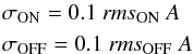 which add up to
  where the term (0.1 CNET)2 accounts for the uncertainty on the photometric calibration.
The errors on the Hα +[NII] flux σF and equivalent width σEW are, finally,  We recall that Eqs. (5) and (6) do not take the uncertainty on the normalisation factor n into account, which might depend on the colour of each galaxy and can be as large as 10% to 30% (Spector et al. 2012). The derived parameters of the observed galaxies are listed in Table 2, arranged as follows:
-
Column 1: HRS name.
-
Column 2: ON-band filter.
-
Column 3: telescope.
-
Column 4: used CCD.
-
Column 5: pixel size in arcseconds.
-
Column 6: observing run.
-
Column 7: number of exposures.
-
Column 8: ON band exposure time per pose in seconds.
-
Column 9: air mass.
-
Column 10: photometric quality of the sky: 1 stands for photometric conditions, 0 unclear conditions (thin cirrus).
-
Column 11: zero point of the observations in erg cm-2 s-1.
-
Column 12: normalisation factor n between the ON- and the OFF-band (r-Gunn) filters.
A few galaxies have been observed during different observing runs. For these galaxies, Table 2 gives a mean value.
CAS parameters for HRS galaxies.
Comparison with the literature.
 |
Fig. 2 Images of six galaxies observed in Hα. The OFF-band contours are logarithmically drawn at 3, 9, 27, and 81 × σ of the sky background in the OFF frame and the grey scales represent the NET flux intensity between 1 and 5 × σ of the sky in the NET frame. A 1 arcmin bar is given on all images. North is up and east is to the left. |
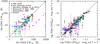 |
Fig. 3 Comparison of the Hα+[NII] equivalent widths (left) and fluxes (right) of the HRS galaxies with independent measurements available in the literature. Red filled dots indicate galaxies with multiple observations done in this work, blue filled dots galaxies with data already published by our team (Boselli & Gavazzi 2002; Boselli et al. 2002; Gavazzi et al. 2002, 2006), magenta, green, cyan, and black symbols Hα+[NII] measurements from Sánchez-Gallego et al. (2012), Kennicutt & Kent (1983; corrected by a factor of 16% as suggested by Kennicutt et al. 1994), Romanishin (1990), or from other references in the literature, respectively. The solid line shows the 1:1 relation. |
4.1. Hα+[NII] data for HRS galaxies
We combine the new set of Hα+[NII] imaging data with those collected in the literature. With our new observations, 281 of the 323 galaxies of the sample now have Hα+[NII] imaging data. The sample is almost complete if limited to late-type systems (254/260 objects, 98%). Table 3 lists the Hα+[NII] equivalent widths and fluxes for the whole HRS sample. Table 3 is arranged as follows:
-
Column 1: HRS name.
-
Columns 2 and 3: Hα+[NII] equivalent width and error in Å.
-
Columns 4 and 5: observed Hα+[NII] flux and error in erg cm-2 s-1.
-
Column 6: reference to the data. When two references are given, the first refers to the equivalent width, the second to the flux. References are coded as follows: TW: this work; 1: Boselli & Gavazzi (2002); 2: Boselli et al. (2002); 3: Gavazzi et al. (2002); 4: Gavazzi et al. (2006); 5: Koopmann et al. (2001); 6: Young et al. (1996); 7: Kennicutt et al. (1987); 8: Macchetto et al. (1996); 9: James et al. (2004); 10: Hameed et al. 2005); 11: Koopmann & Kenney (2006); 12: Usui et al. (1998); 13: Domingue et al. (2003); 14: Trinchieri & Di Serego Alighieri (1991); 15: Finkelman et al. (2010); 16: Kim (1989); 17: Martel et al. (2004); 18: Shields (1991); 19: Singh et al. (1995); 20: Kennicutt & Kent (1983); 21: Romanishin (1990); 22: Sánchez-Gallego et al. (2012); 23: Gallagher & Hunter (1989).
-
Column 7: alternative references, if available.
-
Column 8: notes to individual objects: c indicates that the flux of the galaxy has been determined by indirectly calibrating the image using the published flux of the companion galaxy, m indicates that the published value is a mean value of two independent measurements, and v is for vignetted images where the total flux cannot be properly extracted.
We also determined the Hα+[NII] CAS (concentration, asymmetry, and clumpiness; Conselice 2003) structural parameters for all galaxies with available images. These parameters have been determined following the same procedures as described in Fossati et al. (2013) in both the NET- and the r-band images. These parameters are given in Table 4, arranged as follows:
-
Column 1: HRS name.
-
Columns 2–4: r-band, Hα+[NII], and EWHα + [NII] effective radii in arcsec.
-
Columns 5–7: Concentration, asymmetry, and clumpiness (CAS) parameters from the r-band images.
-
Columns 8–10: Concentration, asymmetry, and clumpiness (CAS) parameters from the Hα+[NII] narrow-band images images.
Figure 2 shows the Hα+[NII] image of six representative galaxies of the sample. All the tables presented in this work, as well as the Hα+[NII] images of the whole sample, will be made available to the community through the HRS dedicated database2.
Fluxes of the emission lines normalised to Hα determined using gandalf.
4.2. Comparison with the literature
Independent sets of data are available for several HRS galaxies (see Table 5). To check the quality of our own measurements and of those collected from the literature, we compare the different sets of published data in Fig. 3. A comparison between the equivalent width of the Hα+[NII] line determined from this set of imaging data with that obtained from integrated spectroscopy has been already presented in Boselli et al. (2013). Figure 3 and Table 5 indicate that the different sets of imaging data give results that are consistent within ≃20% for the equivalent widths and ≃10% for the fluxes. The agreement with the spectroscopic data of Boselli et al. (2013) is within ≃5% (see their Fig. 10). The agreement is good between our independent measurements, or with those obtained by our team during previous observing runs (Boselli & Gavazzi 2002; Boselli et al. 2002; Gavazzi et al. 2002, 2006).
Our new set of data is also consistent with the measurements of Kennicutt & Kent (1983; corrected by a factor of 16% as suggested by Kennicutt et al. 1994 to take a possible contamination of a telluric line in their narrow band filters into account) and Romanishin (1990) done using aperture photometry. They are also fairly consistent with the data recently published by Sánchez-Gallego et al. (2012) or with some other data collected from the literature from a wide variety of references. Figure 3 and Table 5 also show that the uncertainty on the data is generally underestimated using standard error propagation (as recipes given in Eqs. (5) and (6)). One possible reason is that these recipes do not take the contribution from correlated noise into account (which is realistically expected to be a factor of 2–3). Other possible reasons are the photometric uncertainties on the zero-point determination and uncertainties in the continuum subtraction. Overall, the uncertainty on Hα+[NII]EW over the whole HRS dataset is ~66%, while that on the Hα+[NII] flux is ~60%.
5. Determination of the star formation rate
5.1. Dust attenuation correction
As mentioned in the introduction, the Hα emission of late-type star-forming galaxies not dominated by an AGN is due to the gas ionised by the youngest and most massive O-B stars (Kennicutt 1998; Boselli et al. 2001). Under some assumptions on the shape of the IMF and on the star formation history, Hα data can be used to measure the present-day star formation activity of galaxies. To do this, the Hα+[NII] data listed in Table 3 must be corrected to remove the contribution of the two [NII] lines in the narrow band filter and to account for both the Galactic and internal dust attenuation. We first correct the observed Hα+[NII] for the [NII] contamination using an updated version of the long-slit integrated spectroscopic data of the HRS galaxies published in Boselli et al. (2013) (see Appendix A). We then correct them for Galactic extinction using the Schlegel et al. (1998) extinction map combined with the Galactic extinction curve of Fitzpatrick & Massa (2007):  (7)The same set of spectroscopic data is used to estimate the Balmer decrement,
 ![Mathematical equation: \begin{equation} {C({\rm H}\beta) = \frac{{\rm log}(2.86) - {\rm log}\left[\frac{F({\rm H}\alpha)}{F({\rm H}\beta)}\right]_{\rm obs}}{f({\rm H}\alpha)}} , \end{equation}](/articles/aa/full_html/2015/07/aa25712-15/aa25712-15-eq101.png) (8)based on Hα-to-Hβ flux ratio and the Galactic extinction law (f(Hα) = −0.297). The attenuation in the Hα line is then simply given by the relation:
(8)based on Hα-to-Hβ flux ratio and the Galactic extinction law (f(Hα) = −0.297). The attenuation in the Hα line is then simply given by the relation: 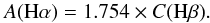 (9)To allow a direct comparison with other works in the literature, we do not apply any further correction for the escape fraction of ionising photons or for the absorption of the ionising radiation by dust (see Boselli et al. 2009 for details).
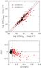 |
Fig. 4 Upper panel: relationship between the Hα luminosity corrected for dust attenuation using the 24 μm luminosity and the prescription of Calzetti et al. (2010) and the Hα luminosity corrected using the Balmer decrement. Black symbols are for galaxies with a σ [C(Hβ)] ≤ 0.1, and red symbols for σ [C(Hβ)] > 0.1. Filled dots are for galaxies with normal gas content (HI-def ≤ 0.4), and empty symbols for gas-poor objects (HI-def > 0.4). The black solid line shows the 1:1 relation, the black long-dashed line the bisector fit (Isobe et al. 1990) determined using the best quality sample (σ [C(Hβ)] ≤ 0.1), while the red dotted line shows the best fit determined using the whole sample. Lower panel: relationship between the distance from the L(Hα)24μ vs. L(Hα)BD relation and the uncertainty on the Balmer decrement estimate σ [C(Hβ)]. The vertical red dashed line shows the limit in σ [C(Hβ)] = 0.1 above which the data are asymmetrically distributed in Δ(y). |
The attenuation in the Hα emission can also be determined using the 24 μm emission combined with one of the several prescriptions given in the literature (Kennicutt et al. 2007, 2009; Calzetti et al. 2007, 2010; Zhu et al. 2008)3. These relations have been calibrated using nearby samples of galaxies with available narrow band Hα+[NII] imaging data, integrated spectroscopy, and mid-infrared data. These data are also available for the HRS sample: WISE 22 μm data for the whole HRS have been recently published by Ciesla et al. (2014). These data can be converted into 24 μm flux densities by multiplying them by a factor of 1.22, as prescribed in Ciesla et al. (2014; see also Boselli et al. 2014d).
5.1.1. Limits in the Balmer decrement determination
Figure 4 shows the relationship between the Hα luminosity corrected for dust attenuation using the 24 μm emission with the prescription of Calzetti et al. (2010) and the Hα luminosity corrected using the Balmer decrement. Only galaxies detected at 22 μm with an available estimate of the [NII]/Hα ratio and of the Balmer decrement are included. The two dependent variables are obviously strongly related. The determination of the Balmer decrement, however, is very uncertain in those objects with a weak Balmer emission, since the contamination of the underlying stellar absorption can be dominant. The lower panel of Fig. 4 shows the relationship between the perpendicular distance from the L(Hα)24 μm vs. L(Hα)BD relation and the uncertainty on the Balmer decrement estimate σ [C(Hβ)] given in Col. 12 of Table 6. Figure 4 shows that the points are symmetrically distributed around the mean relation for σ [C(Hβ)] ≲ 0.1, while they systematically drop below this relation for larger uncertainties on the estimate of the Balmer decrement.
To understand whether this trend is due to a systematic bias in the 24 μm-based dust attenuation correction or in the Balmer decrement-based correction, we compared L(Hα)BD and L(Hα)24 μm to the radio continuum luminosity at 20 cm, which is an independent tracer of the star formation activity in galaxies (e.g. Kennicutt 1998; Bell 2003). At this frequency, the radio continuum emission of galaxies is primarily due to the synchrotron emission of relativistic electrons spinning around weak magnetic fields. These electrons are accelerated in supernova remnants and are thus a direct tracer of the young stellar population (e.g. Boselli 2011). Radio continuum data at 20 cm (1.49 GHz), collected from the literature as explained in Appendix B, are available for 169 (65%) late-type galaxies4. Figure 5 shows that the 20 cm luminosity of the HRS galaxies is tightly correlated with the Hα luminosity. The relation with the Hα luminosity corrected for dust attenuation using the 24 μm band (right panel, σ = 0.15) is less dispersed than the one determined correcting Hα using the Balmer decrement (left panel, σ = 0.20; see Table 8)5. Figure 5 shows, however, that as for the L(Hα)24 μm vs. L(Hα)BD relation shown in Fig. 4, the points are symmetrically distributed around the L(20 cm) vs. L(Hα)BD relation only whenever σ [C(Hβ)] ≲ 0.1, while they drop below the mean relation for higher values of σ [C(Hβ)]. In contrast, the dispersion in the L(20 cm) vs. L(Hα)24 μm relation is symmetric. Figures 4 and 5 consistently indicate that the Balmer decrement is systematically overestimated by ≃0.2 dex (A(Hα) ≃ 0.5 mag) whenever σ [C(Hβ)] ≳ 0.1.
Radio continuum data.
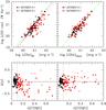 |
Fig. 5 Upper panels: relationship between the 20 cm radio luminosity and the Hα luminosity corrected for dust attenuation using the Balmer decrement (left) and the 24 μm luminosity following the prescription of Calzetti et al. (2010; right). Black symbols are for galaxies with a σ [C(Hβ)] ≤ 0.1, red symbols for σ [C(Hβ)] > 0.1. Filled dots are for galaxies with a normal gas content (HI - def ≤ 0.4), empty symbols for gas-poor objects (HI - def > 0.4). The black short-dashed line in the left panel shows the bisector fit determined using the best quality sample (σ [C(Hβ)] ≤ 0.1), while the red dotted line is the best fit determined using the whole sample. The green long-dashed line gives the bisector fit in the L(20 cm) vs. L(Hα)24 μm relation determined using all galaxies in the right panel. When plotted in the left panel, this fit is close to the one traced by the black dashed line. Lower panels: relationship between the distance from the L(20 cm) vs. L(Hα)BD (left) and the L(20 cm) vs. L(Hα)24 μm relations (right) and the uncertainty on the Balmer decrement estimate σ [C(Hβ)]. |
5.1.2. Limits in the 24 μm dust attenuation correction
The analysis presented in the previous section indicates that Hα luminosities can be accurately corrected for dust attenuation using the Balmer decrement only whenever σ [C(Hβ)] ≲ 0.1. This, however, might introduce systematic biases, in particular in the comparison with the Hα luminosities corrected for dust attenuation using the 24 μm emission. Indeed, as shown in Boselli et al. (2013), the Balmer decrement C(Hβ) is tightly related to the HβEW, thus omitting galaxies with low Hβ emission (thus those with low signal-to-noise in Hβ or equivalently with a large uncertainty on C(Hβ), see Appendix A) might strongly bias the sample towards low attenuated objects. The Hβ emission is also tightly connected to the specific star formation rate. The exclusion of galaxies with low values of Hβ might thus bias the sample towards star-forming, low-mass systems.
It is well known that in these systems, the dust heating sources are mainly young massive stars, while in more quiescent and massive objects, the contribution to the dust heating of the older stellar component might be very important (e.g. Boselli et al. 2006; Cortese et al. 2008; Salim et al. 2009; Bendo et al. 2010, 2012b; Boquien et al. 2011; Boselli et al. 2012). Thus, the calibration of dust attenuation based on the 24 μm emission, taken here as proxy for the total far-infrared luminosity, might not be representative of the most quiescent objects of the sample. To test whether this strong assumption might introduce a systematic bias into the results, we plot in Fig. 6 the relationship between the perpendicular distance from the L(Hα)24 μm vs. L(Hα)BD relation observed in Fig. 4 and different variables characterising the physical properties of the interstellar radiation field of the HRS galaxies. The LTIR, Umin, and γ parameters respectively give the total infrared luminosity, the intensity of the general interstellar radiation field responsible for the heating of the diffuse dust component, and the fraction of dust mass in PDRs heated by the energetic radiation produced by OB associations (Draine et al. 2007). They have been determined by Ciesla et al. (2014), by fitting the infrared SED of the HRS galaxies using the models of Draine & Li (2007). The ratio LTIR/LFUV is a direct tracer of the dust attenuation in galaxies, whereas the γ parameter, the Hβ equivalent width, and the FUV-to-H-band colour index are tracers of the hardness of the radiation field heating the dust. The L24/LTIR quantifies the contribution of the hot dust component to the total far-infrared dust emission of galaxies and is thus tightly connected to the shape of the SED and to the activity of star formation.
Bivariate fit of the luminosity-luminosity relations.
Bivariate fit of the relations between the different Hα and FUV attenuations.
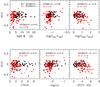 |
Fig. 6 Relationship between the distance from the L(Hα)24 μm vs. L(Hα)BD relation and different parameters characterising the physical properties of the target galaxies, determined as described in the text. Filled dots are for galaxies with a normal gas content (HI - def ≤ 0.4), empty symbols for gas-poor objects (HI - def > 0.4). Black symbols are for galaxies with σ [C(Hβ)] ≤ 0.1, red symbols for σ [C(Hβ)] > 0.1. ρ gives the Spearman correlation coefficient for each panel for the whole sample (black and red; 152 objects) or for galaxies with high signal-to-noise in the spectroscopic data (σ [C(Hβ)] ≤ 0.1; black; 69 objects). |
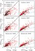 |
Fig. 7 Left column: comparison of A(Hα)24 μm, the attenuation of the Hα measured using different recipes based on the Hα over 24 μm flux ratio, and that determined using the Balmer decrement. Black symbols are for galaxies with σ [C(Hβ)] ≤ 0.1, red symbols for σ [C(Hβ)] > 0.1. Filled dots are for galaxies with a normal gas content (HI - def ≤ 0.4), empty symbols for gas-poor objects (HI - def > 0.4). The black solid lines show the 1:1 relation, the black long-dashed line the bisector fit determined using the best quality sample (σ [C(Hβ)] ≤ 0.1), while the red dotted line indicates the best fit determined using the whole sample. Right: comparison of A(Hα)24 μm and the attenuation A(FUV)24 μm determined in the GALEX FUV band using the prescription of Hao et al. (2011) based on the 24 μm emission band. The blue dotted-dashed line shows the relation expected for a screen model and the Galactic extinction law of Fitzpatrick & Massa (2007), the green short-dashed line the Calzetti attenuation law (Calzetti 2000), and the red dotted line the bisector fit to the data for all galaxies. |
Figure 6 shows that, when all galaxies are considered regardless of the uncertainty on the Balmer decrement, Δ(y) is barely anticorrelated with LTIR/LFUV and (FUV−H)c6 and shows a bimodal distribution when plotted vs. HβEW, L24/LTIR, and γ. In these plots, galaxies with Δ(y) ≲ −0.3/–0.4 all have low values of HβEW (≲5 Å), L24/LTIR (≲0.1), and γ (≲10-2). They also have red (FUV−H)c colours (≳4 mag) and high LTIR/LFUV ratios (≳5). All these properties consistently indicate that galaxies located below the standard L(Hα)24 μm vs. L(Hα)BD relation are relatively quiescent objects where the dust heating is dominated by the evolved stellar population and where dust attenuation is probably important. If confirmed, these trends would indicate a systematic residual in the Hα luminosity correction based on the 24 μm emission, making Eqs. (B.2) and (B.3) non universal since they are only valid for actively star-forming galaxies. We notice, however, that if the same analysis is restricted to those objects with a low uncertainty on the Balmer decrement (σ [C(Hβ)] ≤ 0.1, in Fig. 6), only the trend with L24/LTIR is still statistically significant (the probability that the two variables are correlated is P> 99%). As mentioned above, however, limiting the analysis to galaxies with low uncertainty on the Balmer decrement, thus with high signal-to-noise in the Hα and Hβ lines, might severely bias the sample towards active galaxies. It is thus hard to conclude whether there is a statistically significant indication that the proposed calibration varies with the properties of galaxies. However, it is clear that, as first stressed by Kennicutt et al. (2009), the dust attenuation correction of the Hα emission based on monochromatic far infrared tracers should be used with extreme caution in quiescent massive spiral galaxies.
5.1.3. Comparison between different A(Hα) and A(FUV) estimators
Different recipes have been proposed in the literature to correct Hα luminosities using the 24 μm emission. Figure 7 (and Table 9) shows the relationship between different Hα attenuations determined using these recipes (Calzetti et al. 2010, 2007, and Kennicutt et al. 2009 from top to bottom), and the Hα attenuations determined using the Balmer decrement (left column). All recipes give A(Hα)24 μm ≲ A(Hα)BD regardless of the quality of the spectroscopic data. Among these corrections, however, the one proposed by Calzetti et al. (2010), which uses two different coefficients, one for a starburst regime and one for normal star-forming regions, gives values closest to the 1:1 relation. Whenever the Balmer decrement cannot be determined with high accuracy (σ [C(Hβ)] ≤ 0.1), we adopt this correction in the following analysis. Figure 7 also shows the relationship between A(Hα)24 μm and A(FUV)24 μm determined using the prescription of Hao et al. (2011). Generally, A(Hα)24 μm is ≲A(FUV)24 μm (see however Buat et al. 2002), which is another good reason to prefer the Hα to the the FUV luminosity as a star formation tracer, given that it is less affected by attenuation. The relation between A(Hα)24 μm and A(FUV)24 μm is steeper than the one expected for a simple screen model combined with a Milky Way attenuation curve. This relation is also slightly steeper than the widely used Calzetti law (Calzetti 2001, A(FUV) = 1.86 × A(Hα)) when the Hα attenuation is measured using the prescriptions of Calzetti et al. (2007, 2010), whereas they agree when the Hα attenuation is determined using the prescription of Kennicutt et al. (2009).
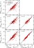 |
Fig. 8 Comparison between the star formation rate determined using different tracers. SFRHα + BD stands for star formation rates determined using Hα luminosities corrected for Balmer decrement (using the gandalf dataset), and SFRHα + 24 μm corrected using the prescription of Calzetti et al. (2010) based on the 24 μm emission. SFRFUV + 24 μm were determined using GALEX FUV data corrected for dust attenuation using the 24 μm emission following Hao et al. (2011), and SFRradio using the 20 cm radio emission following Bell (2003) (see Appendix C). Black symbols are for galaxies with a spectroscopic σ [C(Hβ)] ≤ 0.1, red symbols for galaxies with σ [C(Hβ)] > 0.1. Filled dots are for galaxies with a normal gas content (HI - def ≤ 0.4), empty symbols for gas-poor objects (HI - def > 0.4). The black solid line shows the 1:1 relation, the black dotted line the bisector fit (and σ its dispersion) determined using the best quality sample (σ [C(Hβ)] ≤ 0.1). |
5.2. Star formation rate
5.2.1. Comparison between different tracers
Once corrected for dust attenuation, Hα luminosities can be transformed into star formation rates (SFR, in M⊙ yr-1) using a factor that depends on the assumed IMF and stellar model7:  (10)We recall that this relation is valid only under the assumption that the mean star formation activity of the emitting galaxies is constant on a timescale of a few Myr, roughly comparable to the typical time spent by the stellar population responsible for the ionisation of the gas on the main sequence (Boselli et al. 2009; Boissier 2013; Boquien et al. 2014). The ionising stars are O and early-B stars, whose typical age is ≲107 yr. The stationarity condition is generally satisfied in massive, normal, star-forming galaxies undergoing secular evolution. In these objects, the total number of OB associations is significantly larger than the number of HII regions under formation and of OB stars reaching the final stage of their evolution, thus their total Hα luminosity is fairly constant with time. This might not be the case in strongly perturbed systems or in dwarf galaxies, where the total star formation activity can be dominated by individual giant HII regions (Boselli et al. 2009; Weisz et al. 2012), and the IMF is only stochastically sampled (Lee et al. 2009; Fumagalli et al. 2011; da Silva et al. 2014). The HRS sample is dominated by relatively massive galaxies undergoing secular evolution. For these objects, Eq. (10) can thus be applied. The sample, however, also includes galaxies in the Virgo cluster region, where the perturbation induced by the cluster environment might have affected their star formation rate (e.g. Boselli & Gavazzi 2006, 2014). Models and simulations have shown that in these objects the suppression of star formation occurs on timescales of a few hundred Myr (Boselli et al. 2006, 2008a,b, 2014d). These timescales are relatively long compared to the typical age of O-B stars. The recent work of Boquien et al. (2014) has clearly shown that the Lyman continuum emission tightly follows the rapid variations in the star formation activity of simulated galaxies down to timescales of a few Myrs. We can thus safely consider that the linear relation between the Hα luminosity and the star formation rate given in Eq. (10) is satisfied in the HRS sample.
Star formation rates.
Figure 8 shows the relationship between the star formation rate determined using different tracers: the Hα luminosity, corrected for dust attenuation using both the Balmer decrement and the 24 μm emission; the FUV GALEX luminosities corrected using the 24 μm emission; and the 20 cm radio continuum luminosity. For consistency, all SFR have been measured using the Kennicutt (1998) prescriptions based on a similar IMF (Salpeter in the stellar mass range 0.1 <mstar< 100 M⊙). For the radio continuum we use the Bell (2003) calibration, which is consistent with those used in the other bands (see Appendix C). The different values of SFR are listed in Table 10.
The different star formation rate calibrations give similar results once determined for star-forming galaxies with low uncertainties in C(Hβ). This result is consistent with what was found in the previous section. When compared to SFRFUV + 24 μm, the dispersion is different when different tracers are used: it is very small when compared to SFRHα + 24 μm and gradually increases with SFRHα + BD (when limited to σ [C(Hβ)] ≤ 0.1) and SFRradio (see Table 11). This increase in the dispersion in the relations can be naturally explained by considering that some variables are not fully independent. The dispersion in the relation with the radio continuum tracer might also be affected by other physical factors. In fact, the radio continuum emission can be affected by the presence of an AGN. There is also some indication that the radio continuum emission of cluster galaxies is, on average, stronger than that of similar objects in the field (Gavazzi et al. 1991; Gavazzi & Boselli 1999a,b). The increase in the radio continuum activity of cluster galaxies has been interpreted as due to the compression of the magnetic field during their interaction with the dense intergalactic medium (e.g. Boselli & Gavazzi 2006).
Out of the 260 late-type galaxies in the HRS sample, 196 have more than one empirical determination of the SFR. Figure 9 shows that the typical dispersion σ in the different tracers is of the order of 24%, while the statistical error  in the final SFR is of the order of 14%8. Besides the uncertainty in the data, a part of this scatter can be due to the possibility that the star formation rate tracers based on the FUV and radio luminosities are seriously affected by the stationarity conditions needed to transform luminosities into star formation rates are not always being satisfied, as clearly indicated by Boquien et al. (2014).
5.2.2. Comparison with SED fitting estimates
The star formation activity of galaxies can also be estimated by fitting their observed SED with stellar population synthesis models. An energetic balance between the absorbed stellar radiation and the energy emitted in the far-infrared domain quantifies dust attenuation, allowing determination of several physical parameters of the studied galaxies, such as the stellar mass and the star formation rate (GRASIL, Silva et al. 1998; MAGPHYS, da Cunha et al. 2008; CIGALE, Noll et al. 2009). SED fitting has several advantages with respect to the star formation rate determination based on monochromatic fluxes used in the previous section. First of all, it uses several spectrophotometric bands simultaneously, thus significantly reducing the observational uncertainty on the data. Thanks to a self consistent determination of the dust attenuation, SED fitting also provides several physical parameters (SFR, Mstar, Z, etc.) suitable for any kind of statistical analysis. The SED fitting technique, however, also has several weaknesses. First of all, the output of the SED fitting depends on the star formation history of the galaxy, which is parametrised using simple analytic prescriptions. These are typically not optimised to reproduce the abrupt truncation of the star formation activity that occurred in cluster galaxies (e.g. Boselli & Gavazzi 2006, 2014). SED fitting is generally done by assuming a constant (and fixed) metallicity. The star formation rate derived by SED fitting also depends on the adopted population synthesis models and IMF, as in the case of the monochromatic-based estimates.
Bivariate fit of the relations between the different star formation tracers.
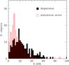 |
Fig. 9 Distribution of the dispersion σ in the different star formation rate tracers (black histogram) and the statistical error ( |
It is thus worth comparing the star formation rate determined using a SED fitting code to the one derived directly from monochromatic fluxes as described in the previous section. To do this, we ran the CIGALE code (Noll et al. 2009; Burgarella et al., in prep.; Boquien et al., in prep.) on all the HRS galaxies. The far-infrared part of the spectrum is fitted using the Draine & Li (2007) dust models, as extensively described in Ciesla et al. (2014). The UV-visible-near-infrared part of the spectrum is fitted using Bruzual & Charlot (2003) stellar population models and assuming a Salpeter IMF and solar metallicity, which is consistent with our approach for the monochromatic determinations. The HRS sample is ideally suited to SED fitting since multifrequency data (including 15 photometric bands) are available for the vast majority of the galaxies. For the present work, we limit the comparison to those galaxies with available GALEX FUV data. Although nebular emission lines can be added to the stellar continuum emission, we do not use them in the present fit, because we want to be representative of the typical data generally used in the SED fitting of galaxies extracted from cosmological surveys.
To remove any possible dependence on short timescale variations in the star formation activity of cluster galaxies, we use the Hα luminosity as a monochromatic tracer (Boquien et al. 2014). Whenever possible (σ [C(Hβ)] ≤ 0.1), we correct it for dust attenuation using the Balmer decrement, otherwise using the 24 μm emission. A 24 μm-based correction might indeed introduce systematic age effects since the dust emitting at this wavelength might be heated by stars older than those responsible for the ionisation of the gas (e.g. Bendo et al. 2012b). The variable SFRHα is available for 196/260 of the late-type galaxies of the sample.
Figure 10 shows the relationship between the star formation rate determined using the SED fitting procedure and the one derived from the Hα luminosity. The SED-fitting estimates have been determined using three commonly-used parametrisations of the star formation history of galaxies: a single exponentially declining law, ![Mathematical equation: \begin{equation} {SFR(t) \propto \exp(-t/\tau_1) ~~~[0.5 \leq \tau_1 \leq 100 ~\rm{Gyr}]} ; \end{equation}](/articles/aa/full_html/2015/07/aa25712-15/aa25712-15-eq178.png) (11)a double exponentially declining law,
(11)a double exponentially declining law, ![Mathematical equation: \begin{equation} SFR(t) = \begin{cases} \exp{-t/\tau_1} & \text{if } t < t_1 - t_2 \\ \exp{-t/\tau_1} + k \times \exp{-t/\tau_2} & \text{if } t \geq t_1 - t_2\\ [0.5 \leq \tau_1 \leq 20 ~\rm{Gyr}; ~~\tau_2 \rightarrow \infty] \end{cases} ; \end{equation}](/articles/aa/full_html/2015/07/aa25712-15/aa25712-15-eq179.png) (12)and a delayed star formation history,
(12)and a delayed star formation history, ![Mathematical equation: \begin{equation} {SFR(t) \propto t \times \exp(-t/\tau_1) ~~~[0.5 \leq \tau_1 \leq 20 ~\rm{Gyr}]} , \end{equation}](/articles/aa/full_html/2015/07/aa25712-15/aa25712-15-eq180.png) (13)where τ are the folding times. These star formation rates are given in Table 10. For the three fits we make the reasonable assumption that galaxies are coeval (13 Gyrs old). Overall, the three star formation rate estimates determined with the SED-fitting code give results consistent with those determined using Hα, as already found in other samples of local or high-z galaxies (e.g. Wuyts et al. 2009; Pforr et al. 2012; Buat et al. 2014)9. This is expected for several reasons: First of all, the single exponentially declining and delayed star formation histories are smooth with respect to time and do not have major changes in the last hundred megayears. They thus correspond to the stationarity condition (SFH = constant) assumed for the monochromatic determination. Second, the HRS galaxies are mainly massive galaxies that underwent a secular evolution. The sample, indeed, does not include strong starbursts or recent mergers, where the star formation activity might have changed abruptly with time. We notice, however, that the SED-fitting-derived star formation activities of the most HI-deficient galaxies are generally lower than those determined using Hα luminosities. These are also objects where the quality of the fit is lower than the average (normalised
(13)where τ are the folding times. These star formation rates are given in Table 10. For the three fits we make the reasonable assumption that galaxies are coeval (13 Gyrs old). Overall, the three star formation rate estimates determined with the SED-fitting code give results consistent with those determined using Hα, as already found in other samples of local or high-z galaxies (e.g. Wuyts et al. 2009; Pforr et al. 2012; Buat et al. 2014)9. This is expected for several reasons: First of all, the single exponentially declining and delayed star formation histories are smooth with respect to time and do not have major changes in the last hundred megayears. They thus correspond to the stationarity condition (SFH = constant) assumed for the monochromatic determination. Second, the HRS galaxies are mainly massive galaxies that underwent a secular evolution. The sample, indeed, does not include strong starbursts or recent mergers, where the star formation activity might have changed abruptly with time. We notice, however, that the SED-fitting-derived star formation activities of the most HI-deficient galaxies are generally lower than those determined using Hα luminosities. These are also objects where the quality of the fit is lower than the average (normalised  ).
).
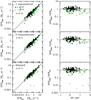 |
Fig. 10 Left panels: the comparison between the star formation rate determined using a SED fitting technique and the one determined using the Hα emission. For the SED fitting determination, all galaxies are assumed to be 13 Gyr old. Three different parametric star formation histories are assumed: exponential (upper panel), double exponential (middle), and delayed (lower). Green symbols indicate those objects where the normalised |

As extensively discussed in Boselli & Gavazzi (2006, 2014), Boselli et al. (2006, 2014c,d), Hughes & Cortese (2009), Cortese & Hughes (2009), and Gavazzi et al. (2013b), the HI-deficiency parameter is tightly connected to the perturbation that affected cluster galaxies. The gas removal resulting from this interaction quenched the activity of star formation on relatively short timescales, in particular in low-mass systems (~100 Myr). On these timescales, the Hα luminosity can still be used as an accurate tracer of the star formation rate of the perturbed galaxies (Boquien et al. 2014). In contrast, the parametric star formation histories adopted for the fit are not optimised to reproduce this rapid truncation of the star formation activity in the gas-stripped cluster galaxies. It is thus conceivable that in these objects, the SED fitting gives less accurate SFR than in unperturbed systems (HI - def ≤ 0.4). Intuitively, however, we would expect an opposite effect since the adopted smooth star formation history would overestimate, rather than underestimate, the current star formation rate. Tests and simulations done so far on observed or mock catalogues of galaxies consistently indicate that the star formation rates determined using SED fitting codes are accurate regardless of the use of different parametrisations or the bursty nature of their evolution (Wuyts et al. 2009; Pforr et al. 2012; Buat et al. 2014; Ciesla et al. 2015). The departure of the HI-deficient galaxies from the one-to-one relation might thus be for other reasons. Indeed, these are quiescent objects characterised by red colours and weak Balmer emission lines, where the contribution of the old stellar population to the dust heating is important. As discussed in Sect. 5.1, the recipes used to determine the Hα attenuation based on the 24 μm emission might introduce systematic effects into the data. To further investigate this intriguing topic, we are planning to use parametric star formation histories defined ad hoc to reproduce the truncated star formation activity of cluster galaxies. The results of this analysis will be presented in a forthcoming paper.
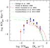 |
Fig. 11 Distribution of the star formation rate in number of galaxies Mpc-3 for the whole HRS late-type galaxies (black dots) and for the subsample of HI-normal (HI - def ≤ 0.4; blue dots) and HI-deficient (HI - def > 0.4; red dots) galaxies. The distribution is compared to several star formation rate luminosity function derived from Hα measurements for the general field. Star formation rates have been determined using the calibration used in this work for a Salpeter IMF. |
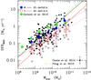 |
Fig. 12 Relationship between the star formation rate and the stellar mass for the HRS late-type galaxies. Filled dots are for HI-normal (HI - def ≤ 0.4) field galaxies, empty circles for HI-deficient (HI - def > 0.4) cluster objects. The large filled blue and empty red circles give the mean values and the standard deviations in different bins of stellar mass determined in this work. The large green filled dots indicate the mean values of Gavazzi et al. (2015a,b). The bisector fit for HI-normal and HI-deficient galaxies are given by the solid black and red lines, and the linear direct fits by the dotted lines. The linear best fit of Ciesla et al. (2014) is indicated by a yellow dashed line, and the best fit of Peng et al. (2010) by the green dotted-dashed line. The error bar shows the typical uncertainty on the data. |
6. Star formation rate properties of the HRS
The complete nature of the HRS, which is volume-limited and K-band-selected, makes it the ideal sample for determining the typical statistical properties of galaxies in the local universe. The completeness in the Hα band has been reached in the late-type systems (Sa-Im-BCD, 98%), so we can derive their statistical properties. The following analysis is thus limited to these star-forming objects. Keeping all the systematic biases in the different tracers analysed in the previous sections in mind, we decided to use the star formation rate determined, whenever possible, by averaging the different monochromatic estimates (SFRHα + BD, SFRHα + 24 μm, SFRFUV + 24 μm, SFRradio ), otherwise using the only one available amongst them. We define this variable SFRMED. In this way we increase the number of galaxies with an available estimate of the SFR from 196/260 (SFRHα) to 236/260 (SFRMED), making the sample complete to 91%. We checked that the results presented in the following section are robust versus the use of different star formation rate tracers.
6.1. Star formation rate distribution
The completeness of the sample allows us to estimate the star formation rate distribution of the HRS. This can be done by counting the number of galaxies in 0.5 dex bins of logSFR (Fig. 11). The normalisation factor is determined assuming that the volume covered by the HRS survey is 4539 Mpc3, consistently with Boselli et al. (2014b) and Andreani et al. (2014). This volume was calculated by considering that, according to the selection criteria described in Boselli et al. (2010)10, we selected galaxies in the volume between 15 and 25 Mpc over an area of 3649 sq.deg. We recall that this is a star formation rate distribution and not a luminosity function since galaxies are first selected in the K band and then counted in bins of SFR. We determined the star formation rate distribution for the whole sample and separately for HI-normal (HI - def ≤ 0.4) and HI-deficient (HI - def > 0.4) galaxies. The former can be considered as typical field sources, while the latter are cluster-perturbed objects (e.g. Boselli & Gavazzi 2006). The star formation rate distribution is compared to several field (Gallego et al. 1995; Tresse & Maddox 1998; Pérez-González et al. 2003; Gunawardhana et al. 2013), star formation rate luminosity functions determined for local galaxies. The Hα luminosity functions have been transformed into star formation rates by adopting the same calibration for a Salpeter IMF and assuming H0 = 70 km s-1 Mpc-1.
Figure 11 shows that the shape of the HRS star formation rate distribution for the whole or for the unperturbed sample is very similar to most of the luminosity functions measured for local galaxies in the literature (maybe with the exception of Pérez-González et al. 2003) for log SFR ≳ −0.5 M⊙ yr-1. For lower values of SFR, the HRS star formation rate distribution drastically drops with respect to the star formation rate luminosity functions published in the literature. This effect is similar to the one observed in the molecular gas mass distribution (Boselli et al. 2014b) of the HRS and can be explained by the incompleteness of the sample at low Hα luminosities. A stellar mass selection (which roughly corresponds to a K-band selection), being the slope of the SFR vs. Mstar relation less then unity (see Fig. 12 and Table 12), excludes low-mass star-forming objects. Using the SFR distribution of mock samples, it has been shown that the star formation rate distribution of a mass-selected sample does not follow the typical Schechter function, but it is better represented by a double Gaussian function with a form close to the one depicted in Fig. 11 (Salim & Lee 2012). A decrease at the faint end of the Hα luminosity function for Coma, A1367, and Virgo cluster galaxies has been found by Iglesias-Paramo et al. (2002).
Coefficients of the scaling relations: y = ax + b.
Figure 11 also shows that the distribution of the HI-normal, unperturbed objects is above the one drawn by the HI-deficient, cluster galaxies. This observational evidence can be easily explained by the quenching of star formation activity in late-type galaxies entering the cluster. Their interaction with the surrounding medium efficiently removes their atomic and molecular gas component, reducing the amount of gas available to form new stars (e.g. Boselli & Gavazzi 2006, 2014; Cortese & Hughes 2009; Hughes & Cortese 2009; Gavazzi et al. 2013a,b; Boselli et al. 2014c,d). This transformation is particularly efficient in dwarf systems where the shallow gravitational potential well cannot retain the gaseous component anchored to the disc (Boselli et al. 2008a,b, 2014d; Boselli & Gavazzi 2014). Curiously, the distribution of the HI-deficient cluster galaxies above SFR ≃ 1 M⊙ yr-1 is similar to the one determined from the GAMA and SDSS sample of Gunawardhana et al. (2013). We recall, however, that the determination of the total volume sampled by the HRS is quite uncertain, thus if the shape of the luminosity distribution is robustly determined, a shift in the Y-axis cannot be totally excluded.
6.2. Star formation rate scaling relations
We trace the typical star formation rate scaling relations of the HRS. These relations can be compared to those already determined on the same sample for the optical and UV structural parameters (Cortese et al. 2012a), for the atomic (Cortese et al. 2011), molecular, and total gas content (Boselli et al. 2014b), and for the dust component (Cortese et al. 2012b). For a fair comparison with these works, we use the same scaling parameters in the following section: the stellar mass Mstar (taken from Cortese et al. 2012a), the stellar mass surface density μstar, the metallicity 12+log(O/H), and the specific star formation rate SSFR. The star formation rates given in Table 10 have been divided by a factor 1.58 to convert them into the Chabrier (2003) IMF. Stellar masses have been determined using i-band luminosities and g−i colours combined with the prescription of Zibetti et al. (2009). Their typical uncertainty is 0.15 dex11. The stellar surface density μstar is the total stellar mass divided by the circular area defined by the i-band effective radius (the radius enclosing 50% of the total light). Its typical uncertainty is 0.20 dex. Metallicities are taken from Hughes et al. (2013) and are determined using the PP04 O3N2 calibration on [NII] and [OIII] emission lines (Pettini & Pagel 2004) with an uncertainty of 0.13 dex. Specific star formation rates SSFR are defined as the ratio of the star formation rate per unit stellar mass. They correspond to the birthrate parameter b once the typical age of galaxies (here assumed to be of 13 Gyr) and a constant returned gas fraction R of 0.3 (Boselli et al. 2001) is taken into account. The typical uncertainty on this variable is 0.25 dex.
Figure 12 shows the relationship between the star formation rate and the stellar mass for all the HRS galaxies. This scaling relation is often referred in the literature as the main sequence (e.g., Guzmán et al. 1997; Brinchmann & Ellis 2000; Bauer et al. 2005; Bell et al. 2005; Papovich et al. 2006; Reddy et al. 2006; Noeske et al. 2007; Salim et al. 2007; Elbaz et al. 2007; Daddi et al. 2007; Pannella et al. 2009; Rodighiero et al. 2010, 2011; Peng et al. 2010; Karim et al. 2011; Whitaker et al. 2012, 2014; Speagle et al. 2014). This relation is expected since it links two variables that scale with the size of galaxies. What is interesting in this relation is the determination of its slope and intercept and of its dispersion (see Tables 12 and 13). The bisector fit derived for the HRS is similar to the one determined by Peng et al. (2010) for a large sample of SDSS local galaxies, whereas the best linear fit is similar to that determined for the HRS by Ciesla et al. (2014) using different definitions of Mstar and SFR. Figure 12 shows a systematic shift in the relation between HI-normal field and HI-deficient cluster galaxies. The relations determined for the two subsamples have a very similar slope, but the shift in the Y-axis is as large as 0.65 dex. The shift in the main sequence as a function of gas content is consistent with what is observed in higher redshift samples by Tacconi et al. (2013). This trend is predictable from the Schmidt law and is a further confirmation that the activity of star formation is quenched in galaxies stripped of their gaseous content in dense environments (e.g. Boselli & Gavazzi 2006, 2014). This evidence, however, contradicts the results of Peng et al. (2010), who find that there is no significant change in the slope and intercept of the main sequence drawn by galaxies belonging to different density environments. The sample of Peng et al. (2010), however, is composed of star-forming galaxies as defined in Brinchmann et al. (2004), which includes galaxies with high signal-to-noise (SN> 3) in the Hα and Hβ lines. This selection criterion obviously favours active star-forming objects, such as those located in the field, but excludes the typical HI-deficient galaxies in clusters, where the activity of star formation is significantly quenched by the lack of gas. It is indeed known that these objects mainly populate the green valley and are thus, in terms of star formation, intermediate between normal star-forming discs and passive early-type galaxies (Boselli et al. 2008a, 2014c,d; Hughes & Cortese 2009; Cortese & Hughes 2009; Gavazzi et al. 2013a,b).
Figure 13 shows the relationship between the specific star formation rate and the morphological class in late-type systems. Figure 13 shows that the specific star formation rate is fairly constant with morphological type (e.g. Kennicutt et al. 1994). It also shows that gas-deficient galaxies have, on average, lower specific star formation rates than similar objects in the field. The mean value of the specific star formation rate of HI-normal galaxies is SSFR = −10.01 ± 0.41 yr-1, while that of HI-deficient objects is SSFR = −10.52 ± 0.49 yr-1. Mean values for each morphological class and standard deviations are given in Table 14. Again, these results are fully consistent with what has previously been found from the Hα imaging survey of nearby cluster galaxies (Gavazzi et al. 2002, 2006).
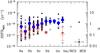 |
Fig. 13 Relationship between the specific star formation rate and the morphological type for HI-normal (HI - def ≤ 0.4; filled dots) and HI-deficient (HI - def > 0.4; empty circles) galaxies. The large filled blue dots indicate the mean values for each morphological class for normal gas-rich systems and the empty red ones for cluster HI-deficient galaxies. For the large symbols, the error bar shows the standard deviation of the distribution. The small error bar shows the typical uncertainty on the data. |
Average scaling relations.
Star formation rate properties as a function of the morphological type.
Figure 14 and Tables 12 and 13 show that the specific star formation rate decreases with increasing stellar mass, stellar surface density, and metallicity (the probability that these variable are correlated is in all cases P> 99.9%). The decrease in the specific star formation rate as a function of the stellar mass has already been noticed in Gavazzi et al. (1998) and explained in the framework of a secular evolution of galaxies in Boselli et al. (2001). It also matches the trend observed in the SDSS for local galaxies (e.g. Brinchmann et al. 2004). The observed trends with the stellar mass surface density and the metallicity occur because Mstar, μstar, and 12 + log(O/H) are tightly connected variables (e.g. Brinchmann et al. 2004; Boselli et al. 2008b; Tremonti et al. 2004). As for Fig. 13, HI-deficient cluster galaxies have, on average, specific star formation rates that are lower than similar field objects with normal HI gas content (Gavazzi et al. 2002, 2006).
6.3. Morphological properties
We can also study how the morphological properties of the HRS late-type galaxies traced by the CAS parameters determined both in the broad band r filter and in the narrow band Hα+[NII] filter are related to the scaling parameters used in the previous section (Figs. 15 and 16). Figure 15 shows that the asymmetry Ar and clumpiness Sr parameters measured in the r band do not change as a function of the stellar mass, stellar surface density, and metallicity of galaxies. The concentration parameter Cr, instead, is fairly constant for galaxies with stellar mass Mstar ≲ 109.5 M⊙ and increases at higher mass. An increase in the concentration index with stellar mass, generally attributed to the presence of a dominant bulge, has been already noticed in the past (e.g. Gavazzi et al. 1996; Fossati et al. 2013). A similar increase in Cr with stellar mass surface density and metallicity is also present and is expected given that all these scaling variables are tightly connected. The three CAS parameters also do not change significantly with the specific star formation rate of galaxies. We notice, however, a very moderate increase in Ar with SSFR.
The same parameters measured in the Hα+[NII] band show much more dispersed distributions and do not show any evident trend when plotted against the stellar mass, stellar mass surface density, and metallicity. Unlike the r-band, the concentration parameter CHα is fairly constant over the whole stellar mass range covered by the sample, consistent with the fact that the star formation activity of galaxies is mainly localised on the disc. Furthermore, the mean values of the three CAS parameters measured in the Hα+[NII] band are systematically shifted with respect to those estimated in the r band, as already noticed by Fossati et al. (2013). A similar increase in the CAS parameters with decreasing wavelength has been also observed by Lauger et al. (2005) and Taylor-Mager et al. (2007) in z ~ 1 galaxies. The CAS parameters are often used to quantify the merging rate of different samples of galaxies (e.g. Conselice 2014). None of the 205 galaxies with available CAS parameters in the r band satisfies the condition 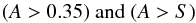 (14)proposed to identify mergers (Conselice 2014). In the Hα band, this condition is satisfied by 7 out of 202 objects (HRS 12, 27, 31, 189, 237, 256, 265), but the clumpy nature of the star-forming regions makes the condition given in Eq. (14) probably not valid in this band.
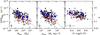 |
Fig. 14 Relationship between the specific star formation rate and the total stellar mass (left), the stellar mass surface density (centre), and the metallicity (right) for HI-normal (HI - def ≤ 0.4; filled dots) and HI-deficient (HI - def > 0.4; empty circles) galaxies. The large filled blue dots indicate the mean values for each morphological class for normal gas-rich systems and the empty red ones for cluster HI-deficient galaxies. For the large symbols the error bar shows the standard deviation of the distribution. The dotted line shows the bisector fit determined for HI-normal galaxies. The small error bar shows the typical uncertainty on the data. |
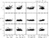 |
Fig. 15 Relationship between the CAS parameters determined in the r band and the total stellar mass (left), the stellar mass surface density (centre left), the metallicity (centre right), and the specific star formation rate (right) for HI-normal (HI - def ≤ 0.4; filled dots) and HI-deficient (HI - def > 0.4; empty circles) galaxies. |
The asymmetry and clumpiness parameters increase systematically with the specific star formation rate SSFR. Galaxies with the highest specific star formation rate, thus those objects that form most of their stars at the present epoch, have a strongly asymmetric distribution of the star-forming regions over their disc. They also have a clumpy structure in Hα+[NII], indicating that their star formation activity is mostly due to giant HII regions sporadically distributed over their discs (distance and blending problems should not introduce strong systematic effects since galaxies are all at ~ the same distance, Thilker et al. 2000; Liu et al. 2013). This result can be explained if the HII region luminosity function and the contribution of the diffuse emission change in galaxies of different stellar mass or morphological type, as first suggested by Kennicutt et al. (1989), Caldwell et al. (1991), and Youngblood & Hunter (1999). These studies have shown that in early-type massive spirals, the bulk of the star formation occurs in several small HII regions, whilst late-type, low-mass systems form most of their massive stars in a few giant HII regions. These results, however, still need to be confirmed on large homogeneous samples with high-quality imaging data (Thilker et al. 2002; Helmboldt et al. 2005; Schombert et al. 2013; Liu et al. 2013). Nevertheless, since the number of HII regions decreases with the decreasing size of galaxies and because their distribution over the disc is random, we expect an increase in the asymmetry parameter in dwarf systems. Variations in the clumpiness index S as a function of the Hα equivalent width, which is a proxy for the SSFR, have already been reported by Conselice (2003), variations of the asymmetry parameter A with the B−V colour index by Conselice et al. (2000).
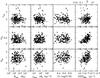 |
Fig. 16 Relationship between the CAS parameters determined in the Hα+[NII] narrow band filter and the total stellar mass (left), the stellar mass surface density (centre left), the metallicity (centre right), and the specific star formation rate (right) for HI-normal (HI - def ≤ 0.4; filled dots) and HI-deficient (HI - def > 0.4; empty circles) galaxies. |
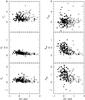 |
Fig. 17 Relationship between the CAS parameters determined in the r (left) and Hα+[NII] narrow band filter (right) and the HI-deficiency parameter for HI-normal (HI - def ≤ 0.4; filled dots) and HI-deficient (HI - def > 0.4; empty circles) galaxies. |
The CAS parameters can also be plotted against the HI-deficiency parameter, which is often taken as a direct tracer of the perturbation induced by the hostile environment in cluster galaxies (e.g. Boselli & Gavazzi 2006). Figure 17 shows that while the CAS parameters measured in the r-band are fairly constant, AHα and SHα systematically decrease with increasing HI-deficiency. Given that HI-deficient galaxies have, on average, lower specific star formation rates than unperturbed systems, this observed decrease might result from the AHα and SHα increase with SSFR observed in Fig. 16.
7. Conclusions
We have presented new Hα+[NII] narrow-band imaging observations of late-type galaxies in the Herschel Reference Survey at the 2.1 m San Pedro Martir telescope. Combined with those already available in the literature, Hα+[NII] data are now available for 281 out of 323 galaxies of the sample and for 254 out of 260 of the late-type systems. These data were used to extract fluxes and equivalent widths, as well as the CAS morphological parameters, with the aim of studying the star formation properties of a volume-limited, K-band-selected complete sample of nearby late-type (Sa-Im-BCD) galaxies. The Hα+[NII] imaging data were first corrected for [NII] contamination and dust attenuation using the integrated spectroscopy and the 24 μm flux densities available for this sample. We then compared the star formation rate determined using either independent monochromatic star formation tracers (Hα, FUV GALEX, radio continuum luminosities) or the output of the CIGALE SED-fitting code done under different assumptions. The comparison of the different tracers shows that:
- 1)
All tracers are strongly correlated with each other (e.g. Calzettiet al. 2007, 2010; Kennicutt et al.2009). The typical dispersion in the derived star formation rates isof the order of 24%. This value, however, should be considered as alower limit for the uncertainty of the SFR determination since it has been determined on variables that are not fully independent and by making similar assumptions on the IMF and on the star formation history of the target galaxies.
- 2)
The Hα luminosities corrected for dust attenuation using the Balmer decrement and the 24 μm emission give consistent results only when the Balmer decrement is determined with an accuracy σ [C(Hβ)] ≤ 0.1. The most distant objects from the L(Hα)BD vs. L(Hα)24 μm relation all have the physical properties typical of quiescent galaxies. This observational evidence suggests that the 24 μm-based attenuation correction derived for star-forming galaxies might not be universal and, as pointed out by Kennicutt et al. (2009), should be used with extreme caution in massive galaxies characterised by a low activity of star formation, where the heating of the dust is also done by the evolved stellar populations.
- 3)
The comparison of the star formation rates determined using monochromatic tracers and UV-to-far-infrared SED fitting codes gives consistent results in unperturbed late-type systems (e.g. Wuyts et al. 2009; Pforr et al. 2012; Buat et al. 2014), while small but systematic differences in the two tracers are present in HI-deficient cluster galaxies. These differences cannot be explained by a non-optimised parametrisation of the star formation history of cluster galaxies that is unable to reproduce an abrupt truncation of their activity once galaxies have entered the cluster. They might be a further indication that the prescription used to correct the Hα for dust attenuation based on the 24 μm emission is not valid in red and quiescent spirals, where the dust heating comes primarily from the evolved stellar population.
Online material
Appendix A: GANDALF spectroscopy
The comparison of the Hα luminosity, corrected for dust attenuation using the Balmer decrement measured in Boselli et al. (2013), and the Hα luminosity, corrected using the 24 μm emission or the 20 cm radio continuum luminosity (Fig. A.1), shows a systematic shift of ~0.5 dex in the relations between galaxies with strong (HβEW > 5 Å) and weak (HβEW < 5 Å) Hβ emission. Given that the three variables are roughly equivalent, the observed shift probably results from a systematic bias in the spectroscopic data used to correct L(Hα)BD.
We recall that in Boselli et al. (2013), the intensity of the Hβ line has been measured by fitting the spectra with a double Gaussian, one for the emission line and the other for the underlying stellar absorption. The observed shift can thus be explained if the Balmer decrement is overestimated or the Hβ emission is underestimated by ~60%. To test whether the observed shift in the relations shown in Fig. A.1 results from a systematic bias introduced by the extraction procedure adopted in Boselli et al. (2013), we extracted the emission line fluxes of all the HRS galaxies with available spectra (Gavazzi et al. 2004; Boselli et al. 2013; 264/323 objects) using the gandalf fitting code (Sarzi et al. 2006; Falcón-Barroso et al. 2006).
gandalf is a simultaneous emission and absorption-line fitting algorithm designed to separate the relative contribution of the stellar continuum and of nebular emission in the spectra of galaxies. This code implements the pPXF method (Cappellari & Emsellem 2004), which combines and adjusts the observed spectra of several stars of all spectral type to the stellar continuum to first quantify and then remove the underlying absorption contaminating the emission of the most important emission lines, including Hβ and Hα. With this procedure, the code is expected to correctly account for the underlying stellar absorption that contaminates several emission lines, in particular the Balmer lines, which are crucial for determining the dust attenuation of the Hα line. Figures 4 and 5 show the same relationships amongst L(Hα)24 μm, L(20 cm), and L(Hα)BD as those plotted in Fig. A.1, but using gandalf data for the Balmer decrement and [NII] contamination corrections. Most of the systematic differences observed between galaxies with high and low HβEW or high and low signal-to-noise are removed using this new set of data. In the analysis presented in this work, we thus use the spectroscopic dataset extracted using gandalf. The fluxes of the different emission lines are given in Table 6, arranged as follows:
-
Column 1: Herschel Reference Sample (HRS) name.
-
Columns 2–8: observed line intensities normalised to Hα. The gandalf fitting code assumes that [OIII]λ4958 = 0.3×[OIII]λ5007 and that [NII]λ6548 = 0.3×[NII]λ6584.
-
Columns 9, 10: signal-to-noise S/N measured empirically from the spectrum as the amplitude of the Hα and Hβ lines divided by the noise in the nearby continuum.
-
Column 11: Balmer decrement C(Hβ). The contribution of the Milky Way is subtracted using the Galactic extinction map of Schlegel et al. (1998) combined with the Fitzpatrick & Massa (2007) Galactic extinction law.
-
Column 12: uncertainty on the Balmer decrement σ [C(Hβ)] obtained from standard error propagation of the uncertainties on the line fluxes.
The uncertainty on the Balmer decrement σ [C(Hβ)] is tightly correlated to the signal-to-noise measured at the Hα and Hβ lines, as depicted in Fig. A.2. For the typical spectral resolution of R ~ 1000 of the spectroscopic data used in this work (Boselli et al. 2013), the required limiting uncertainty of σ [C(Hβ)] = 0.1 is reached for a signal-to-noise of ≃50 for Hα and ≃15 for Hβ. A spectral resolution of R ≳ 1000 is required for an accurate deblending of the Hα line from the nearby [NII] lines and for an accurate determination of the underlying Balmer absorption.
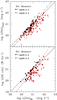 |
Fig. A.1 Relationship between the Hα luminosity corrected for dust attenuation using the 24 μm emission (upper panel), the 20 cm radio continuum luminosity (lower panel), and the Hα luminosity corrected for Balmer decrement using the spectroscopic set of data published in Boselli et al. (2013), where the line emission is directly measured on the data. Filled dots are for HI-normal (HI - def ≤ 0.4) galaxies and empty symbols for HI-deficient (HI - def > 0.4) objects. Black symbols indicate galaxies with an HβEW> 5 Å, red symbols those with HβEW< 5 Å. The black solid line shows the 1:1 relation, the black long dashed line the bisector fit to the high-quality data (black symbols), and the red dotted line the best fit to the whole dataset. |
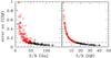 |
Fig. A.2 Relationship between the uncertainty on the Balmer decrement σ [C(Hβ) and the Hα and Hβ signal-to-noise. The horizontal dashed line shows the σ [C(Hβ)] = 0.1 limit adopted in this work to identify good quality objects (black symobls) from uncertain measurements (red symbols). |
Appendix B: Radio continuum data
We have collected radio continuum data at 1.49 GHz (20 cm) obtained at the VLA for 191 HRS galaxies. These data were taken, in order of preference, from the pointed survey of IRAS bright galaxies of Condon et al. (1990), from the survey of optically selected galaxies of Condon (1987), or from the survey of galaxies with the H-band magnitudes of Condon et al. (1987). The data presented in these papers were obtained under similar VLA configurations (generally D and C/D) and thus have a comparable angular resolution (~45 arcsec). The typical rms noise level of these observations is 0.1–0.2 mJy per beam. Flux densities of the remaining galaxies were taken from the NVSS survey of Condon et al. (1998) and published in Condon et al. (2002) whenever available, or extracted by us from the NVSS survey catalogue assuming a search radius of 15 arcsec. These data were homogeneously taken in VLA-D configuration and have a typical resolution of 45 arcsec and a sensitivity of 0.45 mJy rms. For three galaxies, we adopted the integrated flux densities obtained by the FIRST survey (Becker et al. 1995). The FIRST survey was completed using the VLA in B configuration and thus has an angular resolution of ≲5 arcsec. Because of the adopted configuration, this survey is sensitive to compact sources and might miss some of the low surface brightness extended emission. Its typical sensitivity is 0.15 mJy rms.
Table 7 gives the radio data for all the HRS galaxies. Table 7 is arranged as follows:
-
Column 1: Herschel Reference Sample (HRS) name.
-
Column 2: sign indicating detections (1) and non-detections (0).
-
Column 3: flux density S(20 cm) or upper limit in mJy. For the undetected objects, we estimate an upper limit to the flux density Sul(20 cm) = 4 × rms and assume the same typical rms noise of the NVSS survey of 0.45 mJy for all galaxies.
-
Column 4: logarithm of the 20 cm radio luminosity or upper limit in W Hz-1.
-
Column 5: flag to the data, as indicated in the original papers, where 1 stands for galaxies with good quality observations, 2 for uncertain values.
-
Column 6: references to the data: 1: Condon et al. (1990); 2: Condon (1987); 3: Condon et al. (1987); 4: Condon et al. (2002); 5: extracted as described in the text from the NVSS survey (Condon et al. 1998); 6: extracted from the FIRST survey (Becker et al. 1995).
Appendix C: Adopted calibrations of the different star formation tracers
The Hα and FUV star formation rates used in this work were determined using the relation, ![Mathematical equation: \appendix \setcounter{section}{3} \begin{equation} {SFR_{\lambda} ~~~[M_{\odot}{\rm yr}^{-1}] = K_{\lambda} L(\lambda)_{\rm cor} ~~~[\rm erg~s^{-1}] } \end{equation}](/articles/aa/full_html/2015/07/aa25712-15/aa25712-15-eq229.png) (C.1)where the different values of Kλ used in this work are given in Table C.1 (adapted from Hao et al. 2011).
(C.1)where the different values of Kλ used in this work are given in Table C.1 (adapted from Hao et al. 2011).
Calibrations of the different star formation tracers.
The attenuation corrected Hα luminosity have been determined using either the Balmer decrement or the following relation (from Calzetti et al. 2010): ![Mathematical equation: \appendix \setcounter{section}{3} \begin{eqnarray} \log (L({\rm H}\alpha)_{\rm cor}) = \log L({\rm H}\alpha)_{\rm obs} + 0.020 \times \log L(24~\mu{\rm m}) \nonumber\\{\rm for}~~ L(24~\mu{\rm m}) < 10^{42} ~~[\rm{erg \,s^{-1}]} \end{eqnarray}](/articles/aa/full_html/2015/07/aa25712-15/aa25712-15-eq235.png) (C.2)and
(C.2)and ![Mathematical equation: \appendix \setcounter{section}{3} \begin{eqnarray} \log (L({\rm H}\alpha)_{\rm cor}) = \log L({\rm H}\alpha)_{\rm obs} + 0.031 \times \log L(24~\mu{\rm m}) \nonumber\\{\rm for}~~ L(24~\mu{\rm m}) \geq 10^{42} ~~[\rm{erg \,s^{-1}]} \end{eqnarray}](/articles/aa/full_html/2015/07/aa25712-15/aa25712-15-eq236.png) (C.3)where the observed (L(Hα)obs)12 and corrected (L(Hα)cor) Hα luminosities and the 24 μm luminosity (L(24 μm)) are expressed in erg s-1.
(C.3)where the observed (L(Hα)obs)12 and corrected (L(Hα)cor) Hα luminosities and the 24 μm luminosity (L(24 μm)) are expressed in erg s-1.
The corrected UV luminosities are determined using the recipes of Hao et al. (2011):  (C.4)Star formation rates from radio continuum luminosities at 1.49 GHz (20 cm) have been determined using the calibration of Bell (2003):
 ![Mathematical equation: \appendix \setcounter{section}{3} \begin{equation} {SFR_{\rm radio} ~[M_{\odot} \,{\rm yr}^{-1}] = 5.52 \times 10^{-22} L(20~{\rm cm}) ~~{\rm for}~~ L(20~{\rm cm})>L_{\rm c}} \end{equation}](/articles/aa/full_html/2015/07/aa25712-15/aa25712-15-eq241.png) (C.5)
(C.5)![Mathematical equation: \appendix \setcounter{section}{3} \begin{eqnarray} SFR_{\rm radio} ~[M_{\odot} {\rm yr}^{-1}] = \frac{5.52 \times 10^{-22}}{0.1+0.9(L(20~ {\rm cm})/L_{\rm c})^0.3} L(20~{\rm cm}) \nonumber\\{\rm for}~~ L(20~{\rm cm})\leq L_{\rm c} \end{eqnarray}](/articles/aa/full_html/2015/07/aa25712-15/aa25712-15-eq242.png) (C.6)where the radio luminosity is expressed in W Hz-1, and Lc = 6.4 × 10²¹ W Hz-1.
(C.6)where the radio luminosity is expressed in W Hz-1, and Lc = 6.4 × 10²¹ W Hz-1.
The different estimates of the star formation rate are listed in Table 10, arranged as follows:
-
Column 1: Herschel Reference Sample (HRS) name.
-
Column 2: SFRHα + BD determined by correcting the Hα luminosity using the Balmer decrement derived using the gandalf code for galaxies with SN> 50.
-
Column 3: SFRHα + 24 μm determined by correcting the Hα luminosity using the 24 μm emission and Eqs. (C.2) and (C.3).
-
Column 4: SFRFUV + 24 μm determined by correcting the FUV luminosity using the 24 μm emission and Eq. (C4).
-
Column 5: SFRradio determined using the relation C.5 and C.6. This value has been determined only in galaxies with high-quality radio data (flag = 1 in Table 7).
-
Column 6: SFRMED, mean value of the different monochromatic estimates given in Cols. 2–5.
-
Column 7: SFR1exp derived by fitting the SED with the CIGALE code using one exponentially declining star formation history.
-
Column 8: SFR2exp derived by fitting the SED with the CIGALE code using two exponentially declining star formation histories.
-
Column 9: SFRdel derived by fitting the SED with the CIGALE code using a delayed exponentially declining star formation history.
The star formation rates determined using the CIGALE fitting code have been measured only whenever FUV data are available. All galaxies are assumed coeval, with an age of 13 Gyr. We recall that these SFR have been measured assuming consistently a Salpeter IMF in the stellar mass range 0.1 <mstar< 100 M⊙. These values of SFR can be converted into SFR measured using a Chabrier (2003) or Kroupa (2001) IMF by dividing them by a factor of ~1.58. This value changes slightly with the assumed population synthesis model and might vary from reference to reference (Brinchmann et al. 2004; Salim et al. 2007; Bigiel et al. 2008; Argence & Lamareille 2009; Schiminovich et al. 2010; Peng et al. 2010; Chomiuk & Povich 2011).
iraf is distributed by the National Optical Astronomy Observatory, which is operated by the Association of Universities for Research in Astronomy (AURA) under cooperative agreement with the National Science Foundation.
Hα fluxes must first be corrected for Galactic extinction and [NII] contamination as mentioned above.
In the following analysis we consider only galaxies with high-quality radio data (Flag 1 in Table 7).
The less dispersed relation between the radio continuum emission and the Hα luminosity corrected using the 24 μm emission than with the Balmer corrected Hα luminosity might result from the tight connection between the radio and far infrared emission of galaxies (far infrared-radio correlation, de Jong et al. 1985; Condon et al. 1991; Yun et al. 2001; Bell 2003).
The probability that the two variables are correlated is 99 <P< 99.9%.
As mentioned above, we do not apply any correction for any possible escape fraction of the ionising radiation or for the absorption by dust of ionising photons before the ionisation of the gas (see Boselli et al. 2009).
This number underestimates the statistical error since it is based on values of SFR that are not fully independent.
In these works composite star formation histories (exponentially declining plus burst) are often adopted.
The selection conditions are high Galactic latitude (b> +55°) and low Galactic extinction (AB< 0.2 mag) to avoid Galactic cirrus contamination.
We choose to use these stellar masses instead of those determined from SED fitting, which are probably more accurate, because we want to be consistent with all the previous HRS papers presenting the stellar (Cortese et al. 2012a), gas (Cortese et al. 2011; Boselli et al. 2014b), and dust (Cortese et al. 2014) scaling relations.
The observed Hα luminosity must be also corrected for Galactic extinction and [NII] contamination.
Acknowledgments
We are grateful to the referee for constructive comments and suggestions, to Luca Cortese for his long-term collaboration on the HRS project, and to Alessandra Beifiori for useful suggestions on the use of the GANDALF software. This research made use of data from the HRS project. HRS is a Herschel Key Programme utilising guaranteed time from the SPIRE instrument team, ESAC scientists, and a mission scientist. The HRS data was accessed through the Herschel Database in Marseille (HeDaM – http://hedam.lam.fr) operated by CeSAM and hosted by the Laboratoire d’Astrophysique de Marseille. We acknowledge financial support from Programme National de Cosmologie and Galaxies (PNCG) of CNRS/INSU, France. M.F. acknowledges the support of the Deutsche Forschungsgemeinschaft via Project ID 387/1-1. The Hα+[NII] images of the Virgo cluster galaxies belonging to the HRS have been taken from the GOLDMine database (Gavazzi et al. 2003). L.C. acknowledges financial support from the thales project 383549 that is jointly funded by the European Union and the Greek Government in the framework of the programme “Education and lifelong learning”.
References
- Argence, B., & Lamareille, F. 2009, A&A, 495, 759 [NASA ADS] [CrossRef] [EDP Sciences] [Google Scholar]
- Bakes, E. L. O., & Tielens, A. G. G. M. 1994, ApJ, 427, 822 [NASA ADS] [CrossRef] [Google Scholar]
- Bauer, A. E., Drory, N., Hill, G. J., & Feulner, G. 2005, ApJ, 621, L89 [NASA ADS] [CrossRef] [Google Scholar]
- Becker, R. H., White, R. L., & Helfand, D. J. 1995, ApJ, 450, 559 [NASA ADS] [CrossRef] [Google Scholar]
- Bell, E. F. 2003, ApJ, 586, 794 [Google Scholar]
- Bell, E. F., Papovich, C., Wolf, C., et al. 2005, ApJ, 625, 23 [NASA ADS] [CrossRef] [Google Scholar]
- Bendo, G. J., Wilson, C. D., Pohlen, M., et al. 2010, A&A, 518, L65 [NASA ADS] [CrossRef] [EDP Sciences] [Google Scholar]
- Bendo, G. J., Galliano, F., & Madden, S. C. 2012a, MNRAS, 423, 197 [NASA ADS] [CrossRef] [Google Scholar]
- Bendo, G. J., Boselli, A., Dariush, A., et al. 2012b, MNRAS, 419, 1833 [NASA ADS] [CrossRef] [Google Scholar]
- Bigiel, F., Leroy, A., Walter, F., et al. 2008, AJ, 136, 2846 [NASA ADS] [CrossRef] [Google Scholar]
- Binggeli, B., Sandage, A., & Tammann, G. A. 1985, AJ, 90, 1681 [NASA ADS] [CrossRef] [Google Scholar]
- Boissier, S. 2013, in Planets, Stars and Stellar Systems, Vol. 6: Extragalactic Astronomy and Cosmology, 141 [Google Scholar]
- Boselli, A. 2011, A Panchromatic View of Galaxies, Practical Approach Book (Berlin: Wiley-VCH) [Google Scholar]
- Boselli, A., & Gavazzi, G. 2002, A&A, 386, 124 [NASA ADS] [CrossRef] [EDP Sciences] [Google Scholar]
- Boselli, A., & Gavazzi, G. 2006, PASP, 118, 517 [NASA ADS] [CrossRef] [Google Scholar]
- Boselli, A., & Gavazzi, G. 2014, A&ARv, 22, 74 [NASA ADS] [CrossRef] [Google Scholar]
- Boselli, A., Gavazzi, G., Donas, J., & Scodeggio, M. 2001, AJ, 121, 753 [NASA ADS] [CrossRef] [Google Scholar]
- Boselli, A., Iglesias-Páramo, J., Vílchez, J. M., & Gavazzi, G. 2002, A&A, 386, 134 [NASA ADS] [CrossRef] [EDP Sciences] [Google Scholar]
- Boselli, A., Cortese, L., Deharveng, J. M., et al. 2005, ApJ, 629, L29 [NASA ADS] [CrossRef] [Google Scholar]
- Boselli, A., Boissier, S., Cortese, L., et al. 2006, ApJ, 651, 811 [NASA ADS] [CrossRef] [Google Scholar]
- Boselli, A., Boissier, S., Cortese, L., & Gavazzi, G. 2008a, ApJ, 674, 742 [NASA ADS] [CrossRef] [Google Scholar]
- Boselli, A., Boissier, S., Cortese, L., & Gavazzi, G. 2008b, A&A, 489, 1015 [NASA ADS] [CrossRef] [EDP Sciences] [Google Scholar]
- Boselli, A., Boissier, S., Cortese, L., et al. 2009, ApJ, 706, 1527 [NASA ADS] [CrossRef] [Google Scholar]
- Boselli, A., Eales, S., Cortese, L., et al. 2010, PASP, 122, 261 [NASA ADS] [CrossRef] [Google Scholar]
- Boselli, A., Boissier, S., Heinis, S., et al. 2011, A&A, 528, A107 [NASA ADS] [CrossRef] [EDP Sciences] [Google Scholar]
- Boselli, A., Ciesla, L., Cortese, L., et al. 2012, A&A, 540, A54 [NASA ADS] [CrossRef] [EDP Sciences] [Google Scholar]
- Boselli, A., Hughes, T. M., Cortese, L., Gavazzi, G., & Buat, V. 2013, A&A, 550, A114 [NASA ADS] [CrossRef] [EDP Sciences] [Google Scholar]
- Boselli, A., Cortese, L., & Boquien, M. 2014a, A&A, 564, A65 [NASA ADS] [CrossRef] [EDP Sciences] [Google Scholar]
- Boselli, A., Cortese, L., Boquien, M., et al. 2014b, A&A, 564, A66 [NASA ADS] [CrossRef] [EDP Sciences] [Google Scholar]
- Boselli, A., Cortese, L., Boquien, M., et al. 2014c, A&A, 564, A67 [NASA ADS] [CrossRef] [EDP Sciences] [Google Scholar]
- Boselli, A., Voyer, E., Boissier, S., et al. 2014d, A&A, 570, A69 [NASA ADS] [CrossRef] [EDP Sciences] [Google Scholar]
- Boquien, M., Calzetti, D., Combes, F., et al. 2011, AJ, 142, 111 [NASA ADS] [CrossRef] [Google Scholar]
- Boquien, M., Buat, V., & Perret, V. 2014, A&A, 571, A72 [NASA ADS] [CrossRef] [EDP Sciences] [Google Scholar]
- Brinchmann, J., & Ellis, R. S. 2000, ApJ, 536, L77 [NASA ADS] [CrossRef] [Google Scholar]
- Brinchmann, J., Charlot, S., White, S. D. M., et al. 2004, MNRAS, 351, 1151 [NASA ADS] [CrossRef] [Google Scholar]
- Bruzual, G., & Charlot, S. 2003, MNRAS, 344, 1000 [NASA ADS] [CrossRef] [Google Scholar]
- Buat, V., Boselli, A., Gavazzi, G., & Bonfanti, C. 2002, A&A, 383, 801 [NASA ADS] [CrossRef] [EDP Sciences] [Google Scholar]
- Buat, V., Heinis, S., Boquien, M., et al. 2014, A&A, 561, A39 [NASA ADS] [CrossRef] [EDP Sciences] [Google Scholar]
- Caldwell, N., Kennicutt, R., Phillips, A. C., & Schommer, R. A. 1991, ApJ, 370, 526 [NASA ADS] [CrossRef] [Google Scholar]
- Calzetti, D. 2001, PASP, 113, 1449 [NASA ADS] [CrossRef] [Google Scholar]
- Calzetti, D., Kennicutt, R. C., Engelbracht, C. W., et al. 2007, ApJ, 666, 870 [NASA ADS] [CrossRef] [Google Scholar]
- Calzetti, D., Wu, S.-Y., Hong, S., et al. 2010, ApJ, 714, 1256 [NASA ADS] [CrossRef] [Google Scholar]
- Cappellari, M., & Emsellem, E. 2004, PASP, 116, 138 [NASA ADS] [CrossRef] [Google Scholar]
- Chabrier, G. 2003, PASP, 115, 763 [NASA ADS] [CrossRef] [Google Scholar]
- Chomiuk, L., & Povich, M. S. 2011, AJ, 142, 197 [NASA ADS] [CrossRef] [Google Scholar]
- Ciesla, L., Boselli, A., Smith, M. W. L., et al. 2012, A&A, 543, A161 [NASA ADS] [CrossRef] [EDP Sciences] [Google Scholar]
- Ciesla, L., Boquien, M., Boselli, A., et al. 2014, A&A, 565, A128 [Google Scholar]
- Ciesla, L., Charmandaris, V., Georgakakis, A., et al. 2015, A&A, 576, A10 [NASA ADS] [CrossRef] [EDP Sciences] [Google Scholar]
- Condon, J. J. 1987, ApJS, 65, 485 [NASA ADS] [CrossRef] [Google Scholar]
- Condon, J. J. 1992, ARA&A, 30, 575 [NASA ADS] [CrossRef] [MathSciNet] [Google Scholar]
- Condon, J. J., Yin, Q. F., & Burstein, D. 1987, ApJS, 65, 543 [NASA ADS] [CrossRef] [Google Scholar]
- Condon, J. J., Helou, G., Sanders, D. B., & Soifer, B. T. 1990, ApJS, 73, 359 [NASA ADS] [CrossRef] [Google Scholar]
- Condon, J. J., Anderson, M. L., & Helou, G. 1991, ApJ, 376, 95 [NASA ADS] [CrossRef] [Google Scholar]
- Condon, J. J., Cotton, W. D., Greisen, E. W., et al. 1998, AJ, 115, 1693 [NASA ADS] [CrossRef] [Google Scholar]
- Condon, J. J., Cotton, W. D., & Broderick, J. J. 2002, AJ, 124, 675 [NASA ADS] [CrossRef] [Google Scholar]
- Conselice, C. J. 2003, ApJS, 147, 1 [NASA ADS] [CrossRef] [Google Scholar]
- Conselice, C. J. 2014, ARA&A, 52, 291 [NASA ADS] [CrossRef] [Google Scholar]
- Conselice, C. J., Bershady, M. A., & Gallagher, J. S., III 2000, A&A, 354, L21 [NASA ADS] [Google Scholar]
- Cortese, L., & Hughes, T. M. 2009, MNRAS, 400, 1225 [NASA ADS] [CrossRef] [Google Scholar]
- Cortese, L., Boselli, A., Franzetti, P., et al. 2008, MNRAS, 386, 1157 [NASA ADS] [CrossRef] [Google Scholar]
- Cortese, L., Catinella, B., Boissier, S., Boselli, A., & Heinis, S. 2011, MNRAS, 415, 1797 [NASA ADS] [CrossRef] [Google Scholar]
- Cortese, L., Boissier, S., Boselli, A., et al. 2012a, A&A, 544, A101 [NASA ADS] [CrossRef] [EDP Sciences] [Google Scholar]
- Cortese, L., Ciesla, L., Boselli, A., et al. 2012b, A&A, 540, A52 [NASA ADS] [CrossRef] [EDP Sciences] [Google Scholar]
- Cortese, L., Fritz, J., Bianchi, S., et al. 2014, MNRAS, 440, 942 [NASA ADS] [CrossRef] [Google Scholar]
- da Cunha, E., Charlot, S., & Elbaz, D. 2008, MNRAS, 388, 1595 [NASA ADS] [CrossRef] [Google Scholar]
- Daddi, E., Dickinson, M., Morrison, G., et al. 2007, ApJ, 670, 156 [NASA ADS] [CrossRef] [Google Scholar]
- da Silva, R. L., Fumagalli, M., & Krumholz, M. R. 2014, MNRAS, 444, 3275 [NASA ADS] [CrossRef] [Google Scholar]
- de Jong, T., Klein, U., Wielebinski, R., & Wunderlich, E. 1985, A&A, 147, L6 [NASA ADS] [Google Scholar]
- Domingue, D. L., Sulentic, J. W., Xu, C., et al. 2003, AJ, 125, 555 [NASA ADS] [CrossRef] [Google Scholar]
- Draine, B. T., & Li, A. 2007, ApJ, 657, 810 [NASA ADS] [CrossRef] [Google Scholar]
- Draine, B. T., Dale, D. A., Bendo, G., et al. 2007, ApJ, 663, 866 [NASA ADS] [CrossRef] [Google Scholar]
- Dreyer, J. L. E. 1888, MmRAS, 49, 1 [Google Scholar]
- Dreyer, J. L. E. 1895, MmRAS, 51, 185 [NASA ADS] [Google Scholar]
- Elbaz, D., Daddi, E., Le Borgne, D., et al. 2007, A&A, 468, 33 [NASA ADS] [CrossRef] [EDP Sciences] [Google Scholar]
- Falcón-Barroso, J., Bacon, R., Bureau, M., et al. 2006, MNRAS, 369, 529 [NASA ADS] [CrossRef] [Google Scholar]
- Finkelman, I., Brosch, N., Funes, J. G., Kniazev, A. Y., & Vaumlisänen, P. 2010, MNRAS, 407, 2475 [NASA ADS] [CrossRef] [Google Scholar]
- Fitzpatrick, E. L., & Massa, D. 2007, ApJ, 663, 320 [NASA ADS] [CrossRef] [EDP Sciences] [Google Scholar]
- Fossati, M., Gavazzi, G., Savorgnan, G., et al. 2013, A&A, 553, A91 [NASA ADS] [CrossRef] [EDP Sciences] [Google Scholar]
- Fumagalli, M., da Silva, R. L., & Krumholz, M. R. 2011, ApJ, 741, L26 [NASA ADS] [CrossRef] [Google Scholar]
- Gallagher, J. S., III, & Hunter, D. A. 1989, AJ, 98, 806 [NASA ADS] [CrossRef] [Google Scholar]
- Gallego, J., Zamorano, J., Aragon-Salamanca, A., & Rego, M. 1995, ApJ, 455, L1 [NASA ADS] [CrossRef] [Google Scholar]
- Gavazzi, G., & Boselli, A. 1999a, A&A, 343, 93 [NASA ADS] [Google Scholar]
- Gavazzi, G., & Boselli, A. 1999b, A&A, 343, 86 [NASA ADS] [Google Scholar]
- Gavazzi, G., Boselli, A., & Kennicutt, R. 1991, AJ, 101, 1207 [NASA ADS] [CrossRef] [Google Scholar]
- Gavazzi, G., Catinella, B., Carrasco, L., Boselli, A., & Contursi, A. 1998, AJ, 115, 1745 [NASA ADS] [CrossRef] [Google Scholar]
- Gavazzi, G., Boselli, A., Scodeggio, M., Pierini, D., & Belsole, E. 1999, MNRAS, 304, 595 [NASA ADS] [CrossRef] [Google Scholar]
- Gavazzi, G., Boselli, A., Pedotti, P., Gallazzi, A., & Carrasco, L. 2002, A&A, 386, 114 [NASA ADS] [CrossRef] [EDP Sciences] [Google Scholar]
- Gavazzi, G., Boselli, A., Donati, A., Franzetti, P., & Scodeggio, M. 2003, A&A, 400, 451 [NASA ADS] [CrossRef] [EDP Sciences] [Google Scholar]
- Gavazzi, G., Boselli, A., Cortese, L., et al. 2006, A&A, 446, 839 [NASA ADS] [CrossRef] [EDP Sciences] [Google Scholar]
- Gavazzi, G., Fumagalli, M., Galardo, V., et al. 2012, A&A, 545, A16 [NASA ADS] [CrossRef] [EDP Sciences] [Google Scholar]
- Gavazzi, G., Fumagalli, M., Fossati, M., et al. 2013a, A&A, 553, A89 [NASA ADS] [CrossRef] [EDP Sciences] [Google Scholar]
- Gavazzi, G., Savorgnan, G., Fossati, M., et al. 2013b, A&A, 553, A90 [NASA ADS] [CrossRef] [EDP Sciences] [Google Scholar]
- Gavazzi, G., Consolandi, G., Dotti M., et al. 2015a, A&A, in press, DOI: 10.1051/0004-6361/201425351 [Google Scholar]
- Gavazzi, G., Consolandi, G., Viscardi, E., et al. 2015b, A&A, 576, A16 [NASA ADS] [CrossRef] [EDP Sciences] [Google Scholar]
- Groves, B., Brinchmann, J., & Walcher, C. J. 2012, MNRAS, 419, 1402 [NASA ADS] [CrossRef] [Google Scholar]
- Gunawardhana, M. L. P., Hopkins, A. M., Bland-Hawthorn, J., et al. 2013, MNRAS, 433, 2764 [NASA ADS] [CrossRef] [Google Scholar]
- Guzmán, R., Gallego, J., Koo, D. C., et al. 1997, ApJ, 489, 559 [NASA ADS] [CrossRef] [Google Scholar]
- James, P. A., Shane, N. S., Beckman, J. E., et al. 2004, A&A, 414, 23 [NASA ADS] [CrossRef] [EDP Sciences] [Google Scholar]
- Hameed, S., & Devereux, N. 2005, AJ, 129, 2597 [NASA ADS] [CrossRef] [Google Scholar]
- Hao, C.-N., Kennicutt, R. C., Johnson, B. D., et al. 2011, ApJ, 741, 124 [NASA ADS] [CrossRef] [Google Scholar]
- Haynes, M. P., & Giovanelli, R. 1984, AJ, 89, 758 [NASA ADS] [CrossRef] [Google Scholar]
- Helmboldt, J. F., Walterbos, R. A. M., Bothun, G. D., & O’Neil, K. 2005, ApJ, 630, 824 [NASA ADS] [CrossRef] [Google Scholar]
- Hollenbach, D., & Salpeter, E. E. 1971, ApJ, 163, 155 [NASA ADS] [CrossRef] [Google Scholar]
- Hollenbach, D. J., & Tielens, A. G. G. M. 1997, ARA&A, 35, 179 [NASA ADS] [CrossRef] [Google Scholar]
- Hughes, T. M., & Cortese, L. 2009, MNRAS, 396, L41 [NASA ADS] [CrossRef] [Google Scholar]
- Hughes, T. M., Cortese, L., Boselli, A., Gavazzi, G., & Davies, J. I. 2013, A&A, 550, A115 [NASA ADS] [CrossRef] [EDP Sciences] [Google Scholar]
- Karim, A., Schinnerer, E., Martínez-Sansigre, A., et al. 2011, ApJ, 730, 61 [NASA ADS] [CrossRef] [Google Scholar]
- Kennicutt, R. C., Jr. 1998, ARA&A, 36, 189 [Google Scholar]
- Kennicutt, R. C., Jr., & Kent, S. M. 1983, AJ, 88, 1094 [NASA ADS] [CrossRef] [Google Scholar]
- Kennicutt, R. C., & Evans, N. J. 2012, ARA&A, 50, 531 [NASA ADS] [CrossRef] [Google Scholar]
- Kennicutt, R. C., Jr., Roettiger, K. A., Keel, W. C., van der Hulst, J. M., & Hummel, E. 1987, AJ, 93, 1011 [NASA ADS] [CrossRef] [Google Scholar]
- Kennicutt, R. C., Jr., Edgar, B. K., & Hodge, P. W. 1989, ApJ, 337, 761 [NASA ADS] [CrossRef] [Google Scholar]
- Kennicutt, R. C., Jr., Tamblyn, P., & Congdon, C. E. 1994, ApJ, 435, 22 [Google Scholar]
- Kennicutt, R. C., Jr., Calzetti, D., Walter, F., et al. 2007, ApJ, 671, 333 [NASA ADS] [CrossRef] [Google Scholar]
- Kennicutt, R. C., Jr., Lee, J. C., Funes, S. J., et al. 2008, ApJS, 178, 247 [NASA ADS] [CrossRef] [Google Scholar]
- Kennicutt, R. C., Jr., Hao, C.-N., Calzetti, D., et al. 2009, ApJ, 703, 1672 [NASA ADS] [CrossRef] [Google Scholar]
- Kim, D.-W. 1989, ApJ, 346, 653 [NASA ADS] [CrossRef] [Google Scholar]
- Koopmann, R. A., & Kenney, J. D. P. 2006, ApJS, 162, 97 [NASA ADS] [CrossRef] [Google Scholar]
- Koopmann, R. A., Kenney, J. D. P., & Young, J. 2001, ApJS, 135, 125 [NASA ADS] [CrossRef] [Google Scholar]
- Kroupa, P. 2001, MNRAS, 322, 231 [NASA ADS] [CrossRef] [Google Scholar]
- Iglesias-Páramo, J., Boselli, A., Cortese, L., Vílchez, J. M., & Gavazzi, G. 2002, A&A, 384, 383 [NASA ADS] [CrossRef] [EDP Sciences] [Google Scholar]
- Isobe, T., Feigelson, E. D., Akritas, M. G., & Babu, G. J. 1990, ApJ, 364, 104 [NASA ADS] [CrossRef] [EDP Sciences] [Google Scholar]
- Lauger, S., Burgarella, D., & Buat, V. 2005, A&A, 434, 77 [NASA ADS] [CrossRef] [EDP Sciences] [Google Scholar]
- Lee, J. C., Gil de Paz, A., Tremonti, C., et al. 2009, ApJ, 706, 599 [NASA ADS] [CrossRef] [Google Scholar]
- Lequeux, J. 1971, A&A, 15, 42 [NASA ADS] [Google Scholar]
- Lequeux, J., Maucherat-Joubert, M., Deharveng, J. M., & Kunth, D. 1981, A&A, 103, 305 [NASA ADS] [Google Scholar]
- Liu, G., Calzetti, D., Kennicutt, R. C., Jr., et al. 2013, ApJ, 772, 27 [Google Scholar]
- Macchetto, F., Pastoriza, M., Caon, N., et al. 1996, A&AS, 120, 463 [NASA ADS] [CrossRef] [EDP Sciences] [Google Scholar]
- Martel, A. R., Ford, H. C., Bradley, L. D., et al. 2004, AJ, 128, 2758 [NASA ADS] [CrossRef] [Google Scholar]
- Massey, P., Strobel, K., Barnes, J. V., & Anderson, E. 1988, ApJ, 328, 315 [NASA ADS] [CrossRef] [Google Scholar]
- Momcheva, I. G., Lee, J. C., Ly, C., et al. 2013, AJ, 145, 47 [NASA ADS] [CrossRef] [Google Scholar]
- Nilson, P. 1973, Acta Universitatis Upsaliensis, Nova Acta Regiae Societatis Scientiarum Upsaliensis – Uppsala Astronomiska Observatoriums Annaler (Uppsala: Astronomiska Observatorium) [Google Scholar]
- Noeske, K. G., Weiner, B. J., Faber, S. M., et al. 2007, ApJ, 660, L43 [Google Scholar]
- Noll, S., Burgarella, D., Giovannoli, E., et al. 2009, A&A, 507, 1793 [NASA ADS] [CrossRef] [EDP Sciences] [Google Scholar]
- Nolthenius, R. 1993, ApJS, 85, 1 [NASA ADS] [CrossRef] [Google Scholar]
- O’Connell, R. W. 1999, ARA&A, 37, 603 [NASA ADS] [CrossRef] [Google Scholar]
- Osterbrock, D. E., & Ferland, G. J. 2006, Astrophysics of gaseous nebulae and active galactic nuclei, eds. D. E. Osterbrock, & G. J. Ferland (Sausalito, CA: University Science Books) [Google Scholar]
- Pannella, M., Carilli, C. L., Daddi, E., et al. 2009, ApJ, 698, L116 [Google Scholar]
- Papovich, C., Moustakas, L. A., Dickinson, M., et al. 2006, ApJ, 640, 92 [NASA ADS] [CrossRef] [Google Scholar]
- Peng, Y.-j., Lilly, S. J., Kovač, K., et al. 2010, ApJ, 721, 193 [NASA ADS] [CrossRef] [Google Scholar]
- Pérez-González, P. G., Zamorano, J., Gallego, J., Aragón-Salamanca, A., & Gil de Paz, A. 2003, ApJ, 591, 827 [NASA ADS] [CrossRef] [Google Scholar]
- Pettini, M., & Pagel, B. E. J. 2004, MNRAS, 348, L59 [NASA ADS] [CrossRef] [Google Scholar]
- Pforr, J., Maraston, C., & Tonini, C. 2012, MNRAS, 422, 3285 [NASA ADS] [CrossRef] [Google Scholar]
- Reddy, N. A., Steidel, C. C., Fadda, D., et al. 2006, ApJ, 644, 792 [NASA ADS] [CrossRef] [Google Scholar]
- Rodighiero, G., Cimatti, A., Gruppioni, C., et al. 2010, A&A, 518, L25 [NASA ADS] [CrossRef] [EDP Sciences] [Google Scholar]
- Rodighiero, G., Daddi, E., Baronchelli, I., et al. 2011, ApJ, 739, L40 [NASA ADS] [CrossRef] [Google Scholar]
- Romanishin, W. 1990, AJ, 100, 373 [NASA ADS] [CrossRef] [Google Scholar]
- Salim, S., & Lee, J. C. 2012, ApJ, 758, 134 [NASA ADS] [CrossRef] [Google Scholar]
- Salim, S., Rich, R. M., Charlot, S., et al. 2007, ApJS, 173, 267 [NASA ADS] [CrossRef] [Google Scholar]
- Salim, S., Dickinson, M., Michael Rich, R., et al. 2009, ApJ, 700, 161 [NASA ADS] [CrossRef] [MathSciNet] [Google Scholar]
- Sánchez-Gallego, J. R., Knapen, J. H., Wilson, C. D., et al. 2012, MNRAS, 422, 3208 [NASA ADS] [CrossRef] [Google Scholar]
- Sarzi, M., Falcón-Barroso, J., Davies, R. L., et al. 2006, MNRAS, 366, 1151 [NASA ADS] [CrossRef] [Google Scholar]
- Schiminovich, D., Catinella, B., Kauffmann, G., et al. 2010, MNRAS, 408, 919 [NASA ADS] [CrossRef] [Google Scholar]
- Schlegel, D. J., Finkbeiner, D. P., & Davis, M. 1998, ApJ, 500, 525 [NASA ADS] [CrossRef] [Google Scholar]
- Schombert, J., McGaugh, S., & Maciel, T. 2013, AJ, 146, 41 [NASA ADS] [CrossRef] [Google Scholar]
- Shields, J. C. 1991, AJ, 102, 1314 [NASA ADS] [CrossRef] [Google Scholar]
- Silva, L., Granato, G. L., Bressan, A., & Danese, L. 1998, ApJ, 509, 103 [NASA ADS] [CrossRef] [Google Scholar]
- Singh, K. P., Bhat, P. N., Prabhu, T. P., & Kembhavi, A. K. 1995, A&A, 302, 658 [NASA ADS] [Google Scholar]
- Speagle, J. S., Steinhardt, C. L., Capak, P. L., & Silverman, J. D. 2014, ApJS, 214, 15 [NASA ADS] [CrossRef] [Google Scholar]
- Spector, O., Finkelman, I., & Brosch, N. 2012, MNRAS, 419, 2156 [NASA ADS] [CrossRef] [Google Scholar]
- Tacconi, L. J., Neri, R., Genzel, R., et al. 2013, ApJ, 768, 74 [Google Scholar]
- Taylor-Mager, V. A., Conselice, C. J., Windhorst, R. A., & Jansen, R. A. 2007, ApJ, 659, 162 [NASA ADS] [CrossRef] [Google Scholar]
- Thilker, D. A., Braun, R., & Walterbos, R. A. M. 2000, AJ, 120, 3070 [Google Scholar]
- Thilker, D. A., Walterbos, R. A. M., Braun, R., & Hoopes, C. G. 2002, AJ, 124, 3118 [NASA ADS] [CrossRef] [Google Scholar]
- Tremonti, C. A., Heckman, T. M., Kauffmann, G., et al. 2004, ApJ, 613, 898 [NASA ADS] [CrossRef] [Google Scholar]
- Tresse, L., & Maddox, S. J. 1998, ApJ, 495, 691 [NASA ADS] [CrossRef] [Google Scholar]
- Trinchieri, G., & di Serego Alighieri, S. 1991, AJ, 101, 1647 [NASA ADS] [CrossRef] [Google Scholar]
- Tully, R. B. 1987, ApJ, 321, 280 [NASA ADS] [CrossRef] [Google Scholar]
- Usui, T., Saito, M., & Tomita, A. 1998, AJ, 116, 2166 [NASA ADS] [CrossRef] [Google Scholar]
- Valiante, R., Schneider, R., Bianchi, S., & Andersen, A. C. 2009, MNRAS, 397, 1661 [NASA ADS] [CrossRef] [Google Scholar]
- Young, J. S., Allen, L., Kenney, J. D. P., Lesser, A., & Rownd, B. 1996, AJ, 112, 1903 [NASA ADS] [CrossRef] [Google Scholar]
- Youngblood, A. J., & Hunter, D. A. 1999, ApJ, 519, 55 [NASA ADS] [CrossRef] [Google Scholar]
- Yun, M. S., Reddy, N. A., & Condon, J. J. 2001, ApJ, 554, 803 [NASA ADS] [CrossRef] [Google Scholar]
- Waller, W. H. 1990, PASP, 102, 1217 [NASA ADS] [CrossRef] [Google Scholar]
- Weisz, D. R., Johnson, B. D., Johnson, L. C., et al. 2012, ApJ, 744, 44 [NASA ADS] [CrossRef] [Google Scholar]
- Whitaker, K. E., van Dokkum, P. G., Brammer, G., & Franx, M. 2012, ApJ, 754, L29 [NASA ADS] [CrossRef] [Google Scholar]
- Whitaker, K. E., Franx, M., Leja, J., et al. 2014, ApJ, 795, 104 [NASA ADS] [CrossRef] [MathSciNet] [Google Scholar]
- Wolfire, M. G., Hollenbach, D., McKee, C. F., Tielens, A. G. G. M., & Bakes, E. L. O. 1995, ApJ, 443, 152 [Google Scholar]
- Wolfire, M. G., Tielens, A. G. G. M., Hollenbach, D., & Kaufman, M. J. 2008, ApJ, 680, 384 [NASA ADS] [CrossRef] [Google Scholar]
- Wuyts, S., Franx, M., Cox, T. J., et al. 2009, ApJ, 696, 348 [NASA ADS] [CrossRef] [Google Scholar]
- Zhu, Y.-N., Wu, H., Cao, C., & Li, H.-N. 2008, ApJ, 686, 155 [NASA ADS] [CrossRef] [Google Scholar]
- Zibetti, S., Charlot, S., & Rix, H.-W. 2009, MNRAS, 400, 1181 [NASA ADS] [CrossRef] [Google Scholar]
- Zwicky, F., Herzog, E., & Wild, P. 1968, Catalogue of Galaxies and Clusters of Galaxies (Pasadena: California Institute of Technology (CIT)), 1961–1968 [Google Scholar]
All Tables
All Figures
|
Fig. 1 Transmissivity of the ON-band (6603, 6607, 6570 Å) filters. Points indicate the throughput at the wavelength corresponding to the Hα line at the redshift of the target galaxies. |
| In the text | |
|
Fig. 2 Images of six galaxies observed in Hα. The OFF-band contours are logarithmically drawn at 3, 9, 27, and 81 × σ of the sky background in the OFF frame and the grey scales represent the NET flux intensity between 1 and 5 × σ of the sky in the NET frame. A 1 arcmin bar is given on all images. North is up and east is to the left. |
| In the text | |
|
Fig. 3 Comparison of the Hα+[NII] equivalent widths (left) and fluxes (right) of the HRS galaxies with independent measurements available in the literature. Red filled dots indicate galaxies with multiple observations done in this work, blue filled dots galaxies with data already published by our team (Boselli & Gavazzi 2002; Boselli et al. 2002; Gavazzi et al. 2002, 2006), magenta, green, cyan, and black symbols Hα+[NII] measurements from Sánchez-Gallego et al. (2012), Kennicutt & Kent (1983; corrected by a factor of 16% as suggested by Kennicutt et al. 1994), Romanishin (1990), or from other references in the literature, respectively. The solid line shows the 1:1 relation. |
| In the text | |
|
Fig. 4 Upper panel: relationship between the Hα luminosity corrected for dust attenuation using the 24 μm luminosity and the prescription of Calzetti et al. (2010) and the Hα luminosity corrected using the Balmer decrement. Black symbols are for galaxies with a σ [C(Hβ)] ≤ 0.1, and red symbols for σ [C(Hβ)] > 0.1. Filled dots are for galaxies with normal gas content (HI-def ≤ 0.4), and empty symbols for gas-poor objects (HI-def > 0.4). The black solid line shows the 1:1 relation, the black long-dashed line the bisector fit (Isobe et al. 1990) determined using the best quality sample (σ [C(Hβ)] ≤ 0.1), while the red dotted line shows the best fit determined using the whole sample. Lower panel: relationship between the distance from the L(Hα)24μ vs. L(Hα)BD relation and the uncertainty on the Balmer decrement estimate σ [C(Hβ)]. The vertical red dashed line shows the limit in σ [C(Hβ)] = 0.1 above which the data are asymmetrically distributed in Δ(y). |
| In the text | |
|
Fig. 5 Upper panels: relationship between the 20 cm radio luminosity and the Hα luminosity corrected for dust attenuation using the Balmer decrement (left) and the 24 μm luminosity following the prescription of Calzetti et al. (2010; right). Black symbols are for galaxies with a σ [C(Hβ)] ≤ 0.1, red symbols for σ [C(Hβ)] > 0.1. Filled dots are for galaxies with a normal gas content (HI - def ≤ 0.4), empty symbols for gas-poor objects (HI - def > 0.4). The black short-dashed line in the left panel shows the bisector fit determined using the best quality sample (σ [C(Hβ)] ≤ 0.1), while the red dotted line is the best fit determined using the whole sample. The green long-dashed line gives the bisector fit in the L(20 cm) vs. L(Hα)24 μm relation determined using all galaxies in the right panel. When plotted in the left panel, this fit is close to the one traced by the black dashed line. Lower panels: relationship between the distance from the L(20 cm) vs. L(Hα)BD (left) and the L(20 cm) vs. L(Hα)24 μm relations (right) and the uncertainty on the Balmer decrement estimate σ [C(Hβ)]. |
| In the text | |
|
Fig. 6 Relationship between the distance from the L(Hα)24 μm vs. L(Hα)BD relation and different parameters characterising the physical properties of the target galaxies, determined as described in the text. Filled dots are for galaxies with a normal gas content (HI - def ≤ 0.4), empty symbols for gas-poor objects (HI - def > 0.4). Black symbols are for galaxies with σ [C(Hβ)] ≤ 0.1, red symbols for σ [C(Hβ)] > 0.1. ρ gives the Spearman correlation coefficient for each panel for the whole sample (black and red; 152 objects) or for galaxies with high signal-to-noise in the spectroscopic data (σ [C(Hβ)] ≤ 0.1; black; 69 objects). |
| In the text | |
|
Fig. 7 Left column: comparison of A(Hα)24 μm, the attenuation of the Hα measured using different recipes based on the Hα over 24 μm flux ratio, and that determined using the Balmer decrement. Black symbols are for galaxies with σ [C(Hβ)] ≤ 0.1, red symbols for σ [C(Hβ)] > 0.1. Filled dots are for galaxies with a normal gas content (HI - def ≤ 0.4), empty symbols for gas-poor objects (HI - def > 0.4). The black solid lines show the 1:1 relation, the black long-dashed line the bisector fit determined using the best quality sample (σ [C(Hβ)] ≤ 0.1), while the red dotted line indicates the best fit determined using the whole sample. Right: comparison of A(Hα)24 μm and the attenuation A(FUV)24 μm determined in the GALEX FUV band using the prescription of Hao et al. (2011) based on the 24 μm emission band. The blue dotted-dashed line shows the relation expected for a screen model and the Galactic extinction law of Fitzpatrick & Massa (2007), the green short-dashed line the Calzetti attenuation law (Calzetti 2000), and the red dotted line the bisector fit to the data for all galaxies. |
| In the text | |
|
Fig. 8 Comparison between the star formation rate determined using different tracers. SFRHα + BD stands for star formation rates determined using Hα luminosities corrected for Balmer decrement (using the gandalf dataset), and SFRHα + 24 μm corrected using the prescription of Calzetti et al. (2010) based on the 24 μm emission. SFRFUV + 24 μm were determined using GALEX FUV data corrected for dust attenuation using the 24 μm emission following Hao et al. (2011), and SFRradio using the 20 cm radio emission following Bell (2003) (see Appendix C). Black symbols are for galaxies with a spectroscopic σ [C(Hβ)] ≤ 0.1, red symbols for galaxies with σ [C(Hβ)] > 0.1. Filled dots are for galaxies with a normal gas content (HI - def ≤ 0.4), empty symbols for gas-poor objects (HI - def > 0.4). The black solid line shows the 1:1 relation, the black dotted line the bisector fit (and σ its dispersion) determined using the best quality sample (σ [C(Hβ)] ≤ 0.1). |
| In the text | |
|
Fig. 9 Distribution of the dispersion σ in the different star formation rate tracers (black histogram) and the statistical error ( |
| In the text | |
|
Fig. 10 Left panels: the comparison between the star formation rate determined using a SED fitting technique and the one determined using the Hα emission. For the SED fitting determination, all galaxies are assumed to be 13 Gyr old. Three different parametric star formation histories are assumed: exponential (upper panel), double exponential (middle), and delayed (lower). Green symbols indicate those objects where the normalised |
| In the text | |
|
Fig. 11 Distribution of the star formation rate in number of galaxies Mpc-3 for the whole HRS late-type galaxies (black dots) and for the subsample of HI-normal (HI - def ≤ 0.4; blue dots) and HI-deficient (HI - def > 0.4; red dots) galaxies. The distribution is compared to several star formation rate luminosity function derived from Hα measurements for the general field. Star formation rates have been determined using the calibration used in this work for a Salpeter IMF. |
| In the text | |
|
Fig. 12 Relationship between the star formation rate and the stellar mass for the HRS late-type galaxies. Filled dots are for HI-normal (HI - def ≤ 0.4) field galaxies, empty circles for HI-deficient (HI - def > 0.4) cluster objects. The large filled blue and empty red circles give the mean values and the standard deviations in different bins of stellar mass determined in this work. The large green filled dots indicate the mean values of Gavazzi et al. (2015a,b). The bisector fit for HI-normal and HI-deficient galaxies are given by the solid black and red lines, and the linear direct fits by the dotted lines. The linear best fit of Ciesla et al. (2014) is indicated by a yellow dashed line, and the best fit of Peng et al. (2010) by the green dotted-dashed line. The error bar shows the typical uncertainty on the data. |
| In the text | |
|
Fig. 13 Relationship between the specific star formation rate and the morphological type for HI-normal (HI - def ≤ 0.4; filled dots) and HI-deficient (HI - def > 0.4; empty circles) galaxies. The large filled blue dots indicate the mean values for each morphological class for normal gas-rich systems and the empty red ones for cluster HI-deficient galaxies. For the large symbols, the error bar shows the standard deviation of the distribution. The small error bar shows the typical uncertainty on the data. |
| In the text | |
|
Fig. 14 Relationship between the specific star formation rate and the total stellar mass (left), the stellar mass surface density (centre), and the metallicity (right) for HI-normal (HI - def ≤ 0.4; filled dots) and HI-deficient (HI - def > 0.4; empty circles) galaxies. The large filled blue dots indicate the mean values for each morphological class for normal gas-rich systems and the empty red ones for cluster HI-deficient galaxies. For the large symbols the error bar shows the standard deviation of the distribution. The dotted line shows the bisector fit determined for HI-normal galaxies. The small error bar shows the typical uncertainty on the data. |
| In the text | |
|
Fig. 15 Relationship between the CAS parameters determined in the r band and the total stellar mass (left), the stellar mass surface density (centre left), the metallicity (centre right), and the specific star formation rate (right) for HI-normal (HI - def ≤ 0.4; filled dots) and HI-deficient (HI - def > 0.4; empty circles) galaxies. |
| In the text | |
|
Fig. 16 Relationship between the CAS parameters determined in the Hα+[NII] narrow band filter and the total stellar mass (left), the stellar mass surface density (centre left), the metallicity (centre right), and the specific star formation rate (right) for HI-normal (HI - def ≤ 0.4; filled dots) and HI-deficient (HI - def > 0.4; empty circles) galaxies. |
| In the text | |
|
Fig. 17 Relationship between the CAS parameters determined in the r (left) and Hα+[NII] narrow band filter (right) and the HI-deficiency parameter for HI-normal (HI - def ≤ 0.4; filled dots) and HI-deficient (HI - def > 0.4; empty circles) galaxies. |
| In the text | |
|
Fig. A.1 Relationship between the Hα luminosity corrected for dust attenuation using the 24 μm emission (upper panel), the 20 cm radio continuum luminosity (lower panel), and the Hα luminosity corrected for Balmer decrement using the spectroscopic set of data published in Boselli et al. (2013), where the line emission is directly measured on the data. Filled dots are for HI-normal (HI - def ≤ 0.4) galaxies and empty symbols for HI-deficient (HI - def > 0.4) objects. Black symbols indicate galaxies with an HβEW> 5 Å, red symbols those with HβEW< 5 Å. The black solid line shows the 1:1 relation, the black long dashed line the bisector fit to the high-quality data (black symbols), and the red dotted line the best fit to the whole dataset. |
| In the text | |
|
Fig. A.2 Relationship between the uncertainty on the Balmer decrement σ [C(Hβ) and the Hα and Hβ signal-to-noise. The horizontal dashed line shows the σ [C(Hβ)] = 0.1 limit adopted in this work to identify good quality objects (black symobls) from uncertain measurements (red symbols). |
| In the text | |
Current usage metrics show cumulative count of Article Views (full-text article views including HTML views, PDF and ePub downloads, according to the available data) and Abstracts Views on Vision4Press platform.
Data correspond to usage on the plateform after 2015. The current usage metrics is available 48-96 hours after online publication and is updated daily on week days.
Initial download of the metrics may take a while.