| Issue |
A&A
Volume 579, July 2015
|
|
|---|---|---|
| Article Number | A50 | |
| Number of page(s) | 11 | |
| Section | Stellar structure and evolution | |
| DOI | https://doi.org/10.1051/0004-6361/201425393 | |
| Published online | 26 June 2015 | |
Time lags of the flickering in cataclysmic variables as a function of wavelength
Laboratório Nacional de Astrofísica, Rua Estados Unidos 154, 37504-364
Itajubá, Brazil
e-mail: This email address is being protected from spambots. You need JavaScript enabled to view it.
Received: 24 November 2014
Accepted: 3 March 2015
Abstract
Context. Flickering is a ubiquitous phenomenon in cataclysmic variables (CVs). Although the underlying light source is one of the main contributors to the optical radiation, the mechanism leading to flickering is not understood as yet.
Aims. The present study aims to contribute to the set of boundary conditions, defined by observations, which must be met by physical models that describe the flickering. In particular, time lags in the occurrence of flickering events at different wavelengths over the optical range are examined.
Methods. To this end, the cross-correlation functions (CCFs) of numerous light curves of a sample of CVs are analysed that were observed simultaneously or quasi-simultaneously in different bands of various photometric systems.
Results. Deviations of the maxima of the CCFs from zero time-shift indicate a dependence of the flickering activity on the wavelength in the sense that flickering flares reach their maxima slightly earlier in the blue range than in the red. While the available observational material does not permit detecting this individually in all observed systems, the ensemble of all data clearly shows this effect. Particularly instructive are the cases of V603 Aql and TT Ari, where time lags of 15ṣ1 and 4ṣ3, respectively, are observed between the U and R bands. In principle this can be understood if during the development of a flickering flare the radiation characteristics of the light source responsible for flickering change such that in the early phases of a flare more short-wavelength radiation is emitted, and later on, the peak of the emission shifts to the red. Respective scenarios are discussed and shown to be in qualitative and quantitative agreement with observations.
Key words: binaries: close / stars: variables: general / novae, cataclysmic variables
© ESO, 2015
1. Introduction
Cataclysmic variables (CVs) are well known to be short-period interacting binary systems where a Roche-lobe filling star, the secondary, transfers matter via an accretion disk to a white dwarf primary. One of the most striking photometric characteristics common to all CVs are short-term variations of the optical light occurring on time scales of seconds to a few dozen minutes with amplitudes of some hundredths of a magnitude up to more than an entire magnitude. This phenomenon is called flickering and appears to the eye as a continuous sequence of overlapping flares in the light curves of virtually all CVs (but note that this does not necessarily mean that flickering consists of a linear superposition of independent events). Indeed, it can safely be said that if it does not flicker, it is no CV.
Flickering has been observed for more then one and a half centuries: in 1856 Pogson (1857) visually observed variations of the dwarf nova U Gem that might be interpreted as flickering. So did Baxendell in 1858 (Turner 1907). Modern observations of flickering started in the middle of the twentieth century (Henize 1949; Linnell 1950; Lenouvel & Daguillon 1954; Johnson et al. 1954; Walker & Herbig 1954; Walker 1957). The amplitude of the flickering immediately shows that the underlying light source is a major contributor to the optical light of the respective systems. On the mean over all CVs, it emits at least 25% of the radiation of the primary but can easily contribute as much as 50% and in strong flares can outshine the non-flickering light sources even by a factor of almost 2 (Bruch 1989, 1992). Even though flickering is thus due to one of the optically most luminous light sources, it remains among the least understood phenomena observed in CVs.
Flickering is not restricted to CVs or to optical wavelengths. The phenomenon appears rather to be intimately related to accretion of matter from a disk onto a central body. Herbst & Shevchenko (1999), for instance, interpreted flickering-like variations in pre-main-sequence variables as being due to unsteady accretion (see also Kenyon et al. 2000). A comprehensive review of aperiodic X-ray variability in X-ray binaries with neutron stars and black holes was presented by van der Klis (2004). Flickering-like variability also occurs in active galactic nuclei (AGNs; see e.g. Garcia et al. 1999, and references therein). The time scale of the flickering-type variations depends on the dimensions of the underlying system, and the frequency range where it is best observed depends on the compactness of the accretor
The first encompassing systematic study of the flickering properties in CVs has been performed more than two decades ago by Bruch (1989, 1992), who defined several statistical parameters to describe the phenomenon. In addition to quantifying the already mentioned strong contribution of the flickering light source to the total optical light, he showed that the increase of its spectrum to shorter wavelength is steeper than can be explained by simple models such as a black body or a power law. Investigating various physical scenarios, Bruch (1989, 1992) concluded that instabilities in the inner accretion disk and/or the boundary layer between the disk and the white dwarf are most likely to give rise to the observed phenomena.
Later work on flickering includes attempts to identify the exact location where it occurs in CV systems. Already in 1985, Horne & Stiening (1985) had analysed the variations of RW Tri through eclipse and concluded that the flickering light source has the same centre as the accretion disk, but is less extended. This was later confirmed by Bennie et al. (1996). Similarly, Welsh et al. (1996) found that flickering in HT Cas is concentrated to the centre of the disk, but is not confined to the immediate vicinity of the white dwarf. Modifying the technique introduced by Horne & Stiening (1985) to avoid systematic effects, Bruch (1996, 2000) found similar results for several more eclipsing CVs, but that to a lesser degree the hot spot also contributes. However, in IP Peg the hot-spot flickering dominates. In V2051 Oph, Baptista & Bortoletto (2004) identified two flickering components, namely a slowly varying one that they associated with the disk overflowing gas stream from the secondary star, and a more rapidly varying one with a radial distribution equal to the steady disk light.
The behaviour of flickering in the frequency domain has been the subject of many studies. Fritz & Bruch (1998) studied wavelet transforms of numerous light curves of many CVs. They parametrized the resulting scalegrams (Scargle et al. 1993) in terms of its inclination α (frequency behaviour) and its value Σ (flickering strength) at a reference time scale. For a given system, α and Σ are stable over many years. On average, flickering is somewhat bluer on short time-scales than on longer ones. CVs of different types and photometric states occupy distinct regions in the α – Σ – plane. A similar study limited to the intermediate polar V709 Cas was published by Tamburini et al. (2009). A wavelet study in X-rays was performed by Anzolin et al. (2010). The X-ray data are distributed in a much smaller area of the α − Σ parameter space than the optical data. The authors explain the similarity of the X-ray flickering in objects of different classes together with the predominance of a persistent stochastic behaviour in terms of magnetically driven accretion processes acting in a considerable fraction of the analysed objects.
Many studies of the frequency characteristics focus on power spectra where flickering light curves in general exhibit a behaviour similar to red noise, that is, on a double logarithmic scale, a linear decrease of power towards high frequencies (but with a flattening towards low frequencies; Bruch 1989, 1992; Schimpke 1998). Dobrotka et al. (2014) detected two red-noise and two white-noise components in the X-ray power spectrum of RU Peg, indicating the presence of two turbulent regions. The long and low-noise high-cadence light curves of some CVs observed by the Kepler satellite represent superb data from which to study flickering. Scaringi et al. (2012a,b) used these data to construct the flickering power spectrum of MV Lyr, which they decomposed into a broken power law and a series of Lorentzian components, following Belloni et al. (2002) and Nowak et al. (1999). They detected a linear rms – flux relation such that the light source becomes more variable when it becomes brighter, as has earlier been observed in X-ray binaries and AGNs (Uttley & McHardy 2001; Uttley et al. 2005; Heil & Vaughan 2010). This is interpreted as an indication that flickering variations are due to a multiplicative as opposed to an additive process, such as shot noise, since in the latter case the rms – flux relation would be destroyed. In addition to MV Lyr, rapid variations were also analysed in Kepler data of other CVs by Scaringi et al. (2014).
Interpretations of the frequency behaviour in terms of the propagation of disturbances in the accretion disk leading to flickering have repeatedly been discussed in the literature. For instance, Lyubarskii (1997), Yonehara et al. (1997), Pavlidou et al. (2001), and Dobrotka et al. (2010) developed conceptually similar models that differ in details concerning the origin and the propagation of the disturbances. Of these, the model of Lyubarskii (1997), formulated originally to explain X-ray variations in galactic and extragalactic X-ray sources, and which invokes viscosity fluctuations at different radii, has found most widespread attention. In the optical range it has sucessfully been applied to MV Lyr by Scaringi (2014) (but note that Dobrotka et al. 2015, were able to interpret the same observational data also in the framework of the model of Dobrotka et al. 2010). This scenario is quite attractive, in particular because it seeks to explain optical flickering in CVs and X-ray fluctuations in neutron star and black hole binaries as well as AGNs in a unified model. However, it has not yet been convincingly shown that it can explain all flickering characteristics observed in CVs (or, alternatively, that certain properties cited in the literature are based on incorrect assumptions or faulty techniques). Therefore, alternative models should not yet be discarded.
None of these mentioned models is concerned with a detailed description of the emission mechanism that leads to the observed flickering. Of the few attempts to construct a realistic physical model for the temporal and spectral evolution of a flickering flare, the work of Pearson et al. (2005) deserves to be mentioned, which I discuss in more detail in Sect. 5.2.
As a broad-band phenomenon, in the optical range flickering is apparent from the blue to the red atmospheric cutoff and, not surprisingly, in different photometric bands it is not independent from each other but strongly correlated (see, e.g. Fig. 2 of Bruch 1992). However, depending on the temporal evolution of the properties of the emitting light source (e.g. temperature and opacity), it is conceivable that individual flares do not reach their highest intensity simultaneously at all wavelengths, thus leading to time lags between the flickering in different photometric bands. Detection and quantification of such lags will provide constraints on physical mechanisms explaining flickering.
A temporal shift of the flickering at different wavelengths can be traced by measuring the location of the peak of the cross-correlation function (CCF) of light curves in various bands. This technique has been applied by Jensen et al. (1983), who observed in this way a lag of about 1m between the flickering in the optical and X-ray bands in TT Ari. Similarly, Balman & Revnivtsev (2012) detected lags between 96 s and 181 s between UV and X-ray observations in five more CVs. Using optical observations of AM Her, Szkody & Margon (1980) deduced from the asymmetry of the maximum of the CCF a lag of the flickering between the U and B bands of 8 s in the sense that variations appear earlier in U than in B. On the other hand, Bachev et al. (2011) found no conclusive evidence for delays of the flickering in different bands of the nova-like variable KR Aur. This may be due to the comparatively coarse time resolution of 30 s of their data. Bruch (1989, 1992) also obtained null results, but this can probably be attributed to insufficient quality and quantity of the observational data.
A more general approach makes use of the coherence function, that is, a Fourier
frequency-dependent measure of the linear correlation between time series measured
simultaneously in two spectral ranges (Vaughan & Nowak 1997). This permits detecting time lags as a function of the (temporal) frequency
of the underlying signals. This technique has found widespread application in the study of
X-ray binaries and AGNs, but has only recently successfully been applied to optical data of
CVs. Scaringi et al. (2013) studied the
Fourier-frequency-dependent coherence of light curves of MV Lyr and LU Cam observed at high
time resolution (0 844−2276) in the SDSS bands u′, g′ and r′. They also described in
detail the applied data reduction method. Scaringi et al. (2013) found that low-frequency variations (below ≈10-3 Hz) occur about 10 s later in r′ than in u′ in LU Cam. The
corresponding time lag is ≈3 s
in MV Lyr. At higher frequencies, the errors become too large to permit reliable
measurements.
844−2276) in the SDSS bands u′, g′ and r′. They also described in
detail the applied data reduction method. Scaringi et al. (2013) found that low-frequency variations (below ≈10-3 Hz) occur about 10 s later in r′ than in u′ in LU Cam. The
corresponding time lag is ≈3 s
in MV Lyr. At higher frequencies, the errors become too large to permit reliable
measurements.
Here, I investigate numerous light curves of various CVs observed in several photometric systems to measure time shifts of the flickering as a function of wavelength. As mentioned, the time lags observed by Scaringi et al. (2013) are most significant for low-frequency variations. Moreover, the (approximate) power-law behaviour of the flickering power as a function of frequency (Bruch 1989, 1992) means that low-frequency variations strongly dominate high-frequency flickering. Considering furthermore that the CCF will be most sensitive to the strongest variations as well as the limitations of the available data (time resolution, noise, length of individual data sets; see also Sect. 3), I prefer here to use the CCF, which is probably more robust than the much more sophisticated method applied by Scaringi et al. (2013). Not using the coherence function implies the loss of some information. But in view of the data limitation, this disadvantage is compensated by more reliable results than would be possible using more sophisticated techniques. To measure the time lag of the flickering as a function of wavelength, I therefore examine the CCFs of the light curves, that is, the normalized cross covariant as a function of the shift of the data in a reference band with respect to the other (comparison) bands of the photometric system. In Sect. 2 the reduction method is explained. The observational data are briefly introduced in Sect. 3 before the results of this study are presented in Sect. 4. Scenarios to explain the results are discussed in Sect. 5, and finally, conclusions are drawn in Sect. 6.
2. Reduction method
The CCF is calculated in the following way: a light curve is expected to have been sampled
simultaneously in the reference and the comparison band in discrete time intervals separated
by Δt. In the
data sets used in this study this is often the case, but sometimes only approximately so.
Then, the light curves are re-sampled by linear interpolation between data points at the
instances t1 +
j Δt, where t1 is the instance
of the first data point in the reference band, j is an integer number, and Δt is chosen to be the
average time interval between data points in the original light curve. Comparison and
reference data (designated x and y, respectively) are then normalized to their average
value before the mean is subtracted, yielding n pairs of data points (x,y). The CCF is evaluated at
discrete time shifts τk, such that
τk
= k Δt and k is an integral number,
![Mathematical equation: \begin{eqnarray*} {\rm CCF}(\tau_k) = \frac{\sum_{i=1}^m \left( x_i y_{i+k} \right) \, - \, \frac{1}{m}{\sum_{i=1}^m x_i \sum_{i=1}^m y_{i+k}}} {\sqrt{\left[ \sum_{i=1}^m x_i^2 - \frac{\left(\sum_{i=1}^m x_i \right)^2}{m} \right] \left[ \sum_{i=1}^m y_{i+k}^2 - \frac{\left( \sum_{i=1}^m y_{i+k} \right)^2}{m} \right]}}\cdot \end{eqnarray*}](/articles/aa/full_html/2015/07/aa25393-14/aa25393-14-eq27.png) Here, i =
1...m indicate those data pairs for
which reference and comparison data overlap after the comparison data have been shifted in
time by τk. The CCF is thus
discretely sampled at a time resolution of Δt.
Here, i =
1...m indicate those data pairs for
which reference and comparison data overlap after the comparison data have been shifted in
time by τk. The CCF is thus
discretely sampled at a time resolution of Δt.
If reference and comparison data exhibit similar variations but the pattern of variability is shifted by a time interval ts between them, the CCF will assume a maximum at τ = ts ≡ ΔTmax.
In principal, it is straightforward to determine the maximum of the CCF of the data in a reference and a comparison band of light curves observed simultaneously or quasi-simultaneously at different wavelengths. However, there are a few details arising from the structure of the individual data sets available for this study that deserve to be mentioned. As an example, the upper panel of Fig. 1 shows the B band light curve of the old nova V603 Aql observed in the Walraven photometric system on 1983, July 18 (see Walraven & Walraven 1960; and Lub & Pel 1977, for the peculiarities of the Walraven system). In addition to flickering, it shows another feature frequently observed in CVs, that is, variations on longer time scales that may not be immediately associated with flickering (at least not in the light curve discussed here; see Bruch 1991).
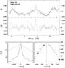 |
Fig. 1 Example of a light curve and the CCF of the brightness variations in two photometric bands. Top: B band light curve of V603 Aql observed on 1983 July 18. The solid line is a fit of a high-order polynomial to the data. Centre: residuals between the original light curve and the polynomial fit. Bottom left: CCF of the light curve shown in the top panel with the simultaneously observed light curve in the U band (broken line) and of the residuals between the original data and the polynomial fit (solid line). Bottom right: enlarged section of the maximum of the CCF shown as a solid line in the lower left panel (dots) together with a fit of a high-order polynomial to the data (broken curve). The broken vertical line indicates the location of the maximum of the fitted polynomial. |
The CCF of the light curves in the B band and the simultaneously observed U band is shown as a broken line in the lower left frame of Fig. 1. The central peak is caused by the correlated flickering activity in the two bands, but on the whole, the profile is rather shallow. This is caused by the longer time-scale modulations. Even if these (in a more general case than for the present example) were a manifestation of flickering, the limited length of the light curves – being of the same order of magnitude – would inhibit a reliable measurement of an associated time lag of the order of a few seconds between different bands. Therefore, to better isolate the variability due to flickering on time scales where a lag can be measured more reliably, it is appropriate to subtract the slow modulations. This is done by fitting a polynomial of suitable order to the original data in both bands, as shown by the solid line in the upper frame of Fig. 1. In all cases when a polynomial was subtracted, the order was chosen such that the polynomial followed the long-term variations satisfactorily, and the same order was adopted for the reference and the comparison bands. The light curve in the central frame of Fig. 1 constitutes the residuals between the original data and the fitted polynomial in the B band. The solid graph in the lower left frame represents the CCF of these residual light curves in B and U. Here, the central peak due to the correlated flickering stands out much more clearly.
The lower right frame of Fig. 1 contains a magnified version of the upper part of the CCF maximum (solid dots). The coarse resolution reflects the rather low time resolution of 21 s of the example light curve. To estimate the location of the maximum, a polynomial was fit to the data of the CCF. Its order depends on the number of available points in the peak of the CCF (range: −120 s ≤ τ ≤ 120 s in this case). This is the dashed line in the figure. In light curves with a very high time resolution, the CCF often contains a sharp spike centred on zero time-shift. It is caused by correlated atmospheric noise in the reference and comparison bands and is masked in the fit process. The quality of the fit indicates that the maximum of the CCF can be determined with high precision by calculating the maximum of the fit polynomial. Its location is marked by the broken vertical line. The corresponding ΔTmax is slightly negative in this example.
To obtain a notion of the accuracy to which ΔTmax can be measured, a simple shot-noise
model was used to generate artificial flickering light curves. While this may not reproduce
the flickering properties observed at least in some CVs and in many X-ray binaries such as
the linear rms − flux relation,
the dependence of the accuray of ΔTmax on properties such as statistical
noise in the data or their time resolution will not depend strongly on such details. Thus,
100 artificial light curves were generated, each of which subsequently served as reference
data. One of them is shown in the upper frame of Fig. 2. The light curves were constructed in the following way: 1500 simulated flares
were distributed randomly on a time base of three hours, which is the typical duration of
the real light curves studied here. Their amplitudes are distributed between
 such that the probability of a flare with a
particular amplitude to occur decays linearly from the minimum to the maximum value of
A and the
probability for a flare with the maximum amplitude goes to zero. The flares are symmetric
and rise and decay at a mean rate of 0
such that the probability of a flare with a
particular amplitude to occur decays linearly from the minimum to the maximum value of
A and the
probability for a flare with the maximum amplitude goes to zero. The flares are symmetric
and rise and decay at a mean rate of 0 5 per hour, allowing for a random scatter
equally distributed between 0 <
dm/ dt ≤ 1 mag per hour around this
value. The superposition of these flares, sampled in 1 s intervals, plus an arbitrary
constant, constitutes the light curves. To make the light curve displayed in Fig. 2 look more natural, random Gaussian noise with
5 per hour, allowing for a random scatter
equally distributed between 0 <
dm/ dt ≤ 1 mag per hour around this
value. The superposition of these flares, sampled in 1 s intervals, plus an arbitrary
constant, constitutes the light curves. To make the light curve displayed in Fig. 2 look more natural, random Gaussian noise with
 was added. Second versions of the same data
sets were created by applying a constant time shift of 5 s to the originals. These served
subsequently as comparison light curves. Using a constant is acceptable here because a
possible dependence of the time lag on flickering frequency as observed in MV Lyr and LU Cam
(Scaringi et al. 2013) will not have a strong bearing
on the accuracy of the ΔTmax determination, the more so because
the CCF is – as mentioned – most sensitive to the stronger low-frequency variations.
was added. Second versions of the same data
sets were created by applying a constant time shift of 5 s to the originals. These served
subsequently as comparison light curves. Using a constant is acceptable here because a
possible dependence of the time lag on flickering frequency as observed in MV Lyr and LU Cam
(Scaringi et al. 2013) will not have a strong bearing
on the accuracy of the ΔTmax determination, the more so because
the CCF is – as mentioned – most sensitive to the stronger low-frequency variations.
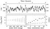 |
Fig. 2 Top: artificial flickering light curve used to estimate the accuracy
of the determination of flickering time lags. Bottom left: dependence
of ΔTmax on the noise level.
Bottom right: expected error of ΔTmax as a
function of the time resolution of the light curve for low
(0 |
To study the accuracy of ΔTmax on the noise level, Gaussian noise was added to the reference and the comparison light curves before ΔTmax was calculated. This was repeated for different noise amplitudes. The results are shown in the lower left frame of Fig. 2, where for each noise level the mean value of ΔTmax derived from the 100 trial light curves is plotted. The error bars are the standard deviation σ around the mean and thus indicate the accuracy with which ΔTmax can be measured in an individual light curve.
The dependence of the accuracy on the time resolution of the data was determined in a
similar way: the artificial light curves were binned to simulate a lower resolution before
noise was added. Then, the standard deviation of ΔTmax was calculated. It is shown in the
bottom right frame of Fig. 2 as a function of the time
resolution for low (002; open circles) and intermediate
(005; filled circles) noise levels.
The accuracy of the results also depends on the length of the light curves (or, equivalently, on the number of data points). Tests with 100 data sets with half (twice) the length of the original ones but with otherwise identical characteristics, subjected to the same noise levels as shown in the lower left frame of Fig. 2, resulted in errors of ΔTmax that were 1.44 ± 0.21 (0.70 ± 0.06) larger. Thus, not unexpectedly, the errors scale to a high degree of accuracy with the inverse of the square root of the length of the light curves.
This exercise shows that ΔTmax can be measured to an accuracy of the order of a tenth of a second in high-quality (long, low noise, high time resolution) light curves, but is limited to several seconds if they are shorter, noisier and/or of low time resolution.
Mean flickering time lags (in seconds) in cataclysmic variables.
3. Data
A total of 197 light curves of 23 different CVs were used in this study. They were observed in several photometric systems over an interval of about two decades at different telescopes by many observers with a variety of scientific purposes in mind. They are thus quite heterogeneous. The data can roughly be grouped and characterized as follows:
VBLUW (Walraven) light curves: they were obtained by various observers at the Dutch telescope at ESO/La Silla, equipped with the Walraven photometer (Walraven & Walraven 1960). The instrument permits only a limited choice of configurations, resulting in a time resolution of about 21 s of the present data, which may be at the limit of usefulness for the current purpose. The five passbands with decreasing wavelengths from V in the visual to W in the ultraviolet are observed simultaneously.
UBV light curves: data in this photometric system were generally observed sequentially in the three bands. This also inhibited a high time resolution. Most of the UBV light curves regarded here are limited to a resolution of ≈15 s or lower.
UBVRI light curves: many suffer from the same disadvantages as their UBV counterparts, resulting thus in a relatively coarse time resolution. However, some have been obtained using a photometer equipped with a rapidly rotating filter wheel (Jablonski et al. 1994), which permits obtaining quasi-simultaneous measurements in all passbands. These data sets were observed at a time resolution of 5 s, and are thus more suitable for the present purpose.
UBVR ∗
(Stiening) light curves: These are data sets were obtained with the Stiening photometer
(Horne & Stiening 1985), which is equipped with
four filters similar but not identical to the standard UBVR filters. All passbands
are observed strictly simultaneously. The disadvantage that this photometric system is not
well calibrated is by far outweighed in the present context by the high time resolution used
to observe the light curves employed here: most have a sampling interval of
05 or 1 s, while some even reach
02.
Thus, the most suitable data sets are those observed at high time resolution in the UBVRI system and, above all, the Stiening data.
4. Results
All available light curves were subjected to the reduction method outlined in Sect. 2. The B band was used as reference band1. The light curves of all other bands were cross-correlated with the B band light curve, and the time lags ΔTmax of the maxima of the respective CCFs were determined. In some cases, only parts of the light curves were used. This applies in particular to AE Aqr, which sometimes exhibits periods of no or very weak flaring activity that were then excluded. Eclipses in some light curves of eclipsing CVs were also removed. Strong long-term variations (time scale: hours), if present, were removed by subtracting a fitted polynomial of suitable degree (see Fig. 1).
Table 1 contains average values of ΔTmax of the maximum of the CCF of each comparison band with respect to the reference band as indicated in the table header. This is interpreted as the time lags of the flickering in these bands. Since short data sets should contribute to the average to a lesser degree than long ones, the results for the individual light curves were weighted with their total duration. The number n of light curves contributing to the mean are given in brackets. The errors are standard deviations derived from all light curves of a given star. No selection was made. All light curves, regardless of the photometric system or the time resolution, enter the average.
4.1. The ensemble
No clear picture emerges for the individual systems. In most cases, the standard deviation is considerable, often significantly larger than the average value of ΔTmax. This is not surprising in view of the expected errors determined from the simulations performed in Sect. 2 and the limited quality of most light curves. Moreover, more often than not (disregarding the errors), there is no monotonical dependency of ΔTmax as a function of wavelength difference between reference and comparison bands, as might be naively expected. However, when the investigated stars are considered as an ensemble, at least a trend appears.
Isophotal wavelengths.
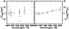 |
Fig. 3 Left: average ΔTmax for all investigated CVs as a function of isophotal wavelength of the comparison band. Right: average ΔTmax of all individual light curves, weighted in proportion to their duration. The broken line is a linear least-squares fit to the data points (excluding the points referring to the W and U bands), weighted by the inverse of their standard deviations. The error bars represent the mean error of the mean. In both frames the location of the reference band (B) is indicated by a cross. |
In Fig. 3 (left) the average ΔTmax for each system is shown as a function of the isophotal wavelength λiso of the comparison band. λiso was calculated using the transmission curves as listed by Bessell (1990) for the UBVRI system and by Lub & Pel (1977) for the Walraven system (applying a correction based on the revision of the mean wavelengths by de Ruiter & Lub 1986), together with a first-order approximation of the spectral density Sλ of a CVs according to the law Sλ ∝ λ− 7 / 3, valid over a wide wavelength range for an accretion disk radiating locally as a black body (Lydnen-Bell 1969). The results are listed in Table 2. Since the transmission curves of the Stiening system are unknown, λiso was taken to be the same as for the respective bands of the UBVRI system. Moreover, for simplicity in the case of the Walraven system the isophotal wavelength of the U, B and V bands were substituted by those of the UBVRI system in Fig. 3. Finally, ΔTmax between the B and R band of the only light curve of UX UMa was discarded because of a very high negative value, deviating strongly from all other results. This is due to a peculiar and highly asymmetric CCF. The location of the (reference) B band (where ΔTmax should evidently be zero) is indicated by a cross in Fig. 3.
There is a certain trend for ΔTmax to increase with wavelength for the photometric bands redward of U, meaning that on average there is a slight offset between the flickering in the blue and in the visual or red or infrared in the sense that flickering occurs later at longer wavelength. But this trend is not continued to the ultraviolet W and U bands. It may not be a coincidence that the points deviating from the linear relationship refer to those bands that have an isophotal wavelength shorter than the Balmer limit (see Sect. 5.2).
The right frame of Fig. 3 is similar to the left
one. However, instead of showing the average ΔTmax values of the respective systems,
the average of all individual light curves, weighted in proportion to their lengths, is
shown as a function of the wavelength of the comparison band. The error bars represent the
mean error of the mean (i.e. the σ/ , where σ is the standard deviation
and n is the
number of data points contributing to the average). The broken line is a linear
least-squares fit (excluding the W and U bands) where the data points were weighted
according to the inverse of the standard deviation. It has an inclination of
(1.9 ± 0.3) ×
10-3 s/Å 2. Again, the
cross indicates the location of the reference band that did not enter the fit.
, where σ is the standard deviation
and n is the
number of data points contributing to the average). The broken line is a linear
least-squares fit (excluding the W and U bands) where the data points were weighted
according to the inverse of the standard deviation. It has an inclination of
(1.9 ± 0.3) ×
10-3 s/Å 2. Again, the
cross indicates the location of the reference band that did not enter the fit.
The trends observed in Fig. 3 suggests the consistent presence of flickering time lags in CVs, but may not yet be considered conclusive evidence. This is the more so because the data points shortward of the Balmer jump deviate from the linear relationship. It may be that well-defined time lags in some system with high-quality data are “diluted” by large errors from lower quality light-curves when regarding the entire ensemble. This is suggested by more convincing results on some individual systems that I discuss subsequently.
4.2. Individual systems
While there is thus a trend for a time lag of the flickering at different wavelengths when regarding the whole ensemble of investigated light curves, this is, as mentioned, in general not evident when regarding individual stars. There are exceptions, however. Concentrating on high-quality, low-noise light curves with a time resolution of ≤5 s and using as criteria (i) that a reasonable number of light curves are available to render the results statistically reliable; (ii) that the standard deviation of the ΔTmax values of the individual curves is significantly smaller than the difference of the average ΔTmax at short and long wavelengths; and (iii) that the average ΔTmax is a monotonic function of wavelength and has a different sign for comparison bands shorter and longer than the reference band, two systems were identified where ΔTmax has a convincing dependence on wavelength. These are V603 Aql and TT Ari.
Restricted results for individual systems.
For both stars, these results are based almost exclusively on the high time resolution UBVR ∗ light curves. Only for V603 Aql, additionally, two UBVRI data sets were used. Table 3 lists the average ΔTmax values together with their statistical errors. The number of contributing light curves is given in brackets. Figure 4 (upper frames), which is organized in the same way as the right frame of Fig. 3, show the same results graphically. Clearly, ΔTmax strictly obeys a linear relationship with wavelength λ, which, in these cases, continues to the U band. The derivative of ΔTmax with respect to λ, that is, the inclination of a linear fit to the data points weighted by the inverse of their standard deviation, is listed in the last line of Table 3.
If I relax the criteria formulated in the first paragraph of this subsection, permitting that in the bands blue-ward of the Balmer jump ΔTmax deviates from a monotonical relationship with wavelength, and including also light curves observed with lower time resolution (but requiring instead that at least four remaining data points are available), Table 1 shows that the relationship between ΔTmax and λ is also quite significant for RS Oph (lower left frame of Fig. 4) for wavelengths longer than the Balmer limit. For this system, the derivative dΔTmax/ dλ = (3.6 ± 0.5) × 10-3 s/Å.
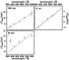 |
Fig. 4 Average ΔTmax derived from high time resolution light curves of V603 Aql, TT Ari and RS Oph as a function of isophotal wavelength of the comparison band. The broken lines are linear least-squares fits to the data points (in the case of RS Oph without considering the points referring to the W and U bands), weighted by the inverse of their standard deviations. The location of the reference band (B) is indicated by a cross. The error bars represent the mean error of the mean. |
dΔTmax/ dλ differs for the three stars, being more than three times higher in V603 Aql than in TT Ari, with the value for RS Oph lying in between. This holds true for the average, but also for inclinations derived from the individual light curves. The magnitude of the flickering time lags thus depends on the particular star, but within a given system it appears to be more or less stable3. However, this statement being based here on only three stars still requires confirmation from high-quality data of other CVs.
Scaringi et al. (2013) found that the time lags in the stars studied by them depend on the frequency of the fluctuations, which are larger for variations occuring on longer time scales (and even may change sign on short time-scales). The CCF technique applied here is not able to distinguish between different temporal frequencies. Therefore, the observed time lags should represent some kind of weighted mean over all time scales. Since the CCF is most sensitive to the strongest variations, the mean is expected to be biased to the time lags of the dominating fluctuations. Bruch (1989, 1992) has shown that in many CVs these occur on time scales of the order of 2 min−4 min as measured from the width of the central peak of the auto-correlation function of their light curves.
The fact that a time lags between the flickering in different photometric bands is clearly measured in the two systems with the highest quality data available for this study (plus at least one additional system (RS Oph) and also the stars observed by Scaringi et al. 2013) gives confidence that the trend observed in the entire ensemble is not accidental, but a strong indication that a similar time lag is a universal feature of the flickering in CVs.
5. Discussion
As mentioned in the introduction, reports about a time lag of the flickering in different spectral regions have been published earlier, but the scope and quantity of these studies remains quite limited. In two older papers and in two more recent studies a positive detection is claimed.
The finding of Szkody & Margon (1980) that in AM Her the flickering in the V band lags that in the U band by 8 s is not based on the measurement of the peak of the CCF, but on its asymmetry. They measured the lag at the half-intensity point. But it is by no means obvious how an asymmetry in the peak of a CCF is related to a time lag between the correlated functions. Indeed, tests with artificial light curves showed that it is not easy to introduce asymmetries in the CCFs by shifting the flares in one of the bands or by changing their shape4. However, such asymmetries can be caused by longer time-scale variations if these are significantly different in the reference and comparison bands. Therefore, it is not clear how reliable the results of Szkody & Margon (1980) are. They interpreted their findings in the framework of the AM Her star model, which does not apply to the CVs studied here.
More relevant in the present connection is the study of Jensen et al. (1983), who found a correlations between the flickering in X-rays and the optical in TT Ari, the same system where I have detected a highly significant dependence of ΔTmax on the wavelength in Sect. 4.2. The X-rays lag the optical variations by about a minute. Jensen et al. (1983) interpreted their results within a model where X-rays are emitted by a corona above the accretion disk. The correlation of variations in the different bands can then be understood as due to the efficiency of acoustic and magneto-hydrodynamic transport processes from the disk to the corona. However, Jensen et al. (1983) did not investigate this scenario quantitatively. Balman & Revnivtsev (2012) obtained similar results for additional CVs, but interpreted them differently: in the framework of a model of propagating fluctuations (e.g., Lyubarskii 1997), the lag would be due to the travel time of matter from the innermost part of a truncated accretion disk to the surface of the white dwarf.
While Szkody & Margon (1980) focused on the special case of a strongly magnetic CV, and Jensen et al. (1983) as well as Balman & Revnivtsev (2012) compared flickering in widely differing wavelength ranges, the study of flickering time delays in MV Lyr and LU Cam by Scaringi et al. (2013) can be compared much more directly to the present one. As mentioned, at low flickering frequencies (several times 10-2 Hz as read from their Fig. 3), they measured a delay of ≈10 s in LU Cam and ≈3 s in MV Lyr of the r′ band variations with respect to those in the u′ band. With the average SDSS filter wavelengths as informed on the SDSS web page (and neglecting the small difference between average and isophotal wavelength), this translates into a time lag of 3.8 × 10⁻³ s/Å and 1.1 × 10⁻³ s/Å, respectively. These numbers are quite similar to the time lags observed here, strengthening the case for such lags to be ubiquitous in CVs.
5.1. A heuristic model
The time lags observed here in the optical bands are much smaller than those seen by Jensen et al. (1983) and Balman & Revnivtsev (2012) and have the opposite wavelength dependence. This is not surprising because the reasons for the lags in the optical bands probably are quite different from those for the lag between the optical and X-ray range. Here, I find that variations in the blue occur slightly earlier than in the red. In principle this can be understood if during the development of a flickering flare the radiation characteristics of the underlying light source change such that in the early phases of the flare more short wavelength radiation is emitted, and later on, the peak of the emission shifts to the red.
To verify that this leads to results that are compatible with the observations, a very simple scenario was investigated. I stress that this is not meant as a physically realistic model but just to show that based on simple but sensible assumptions, it is possible to reproduce the results found in Sect. 4.
For this purpose the light source underlying a flickering flare was approximated by a
black body with a temperature Θ 5 that over time
t varies
according to some function Θ(t). The emitting area
 of the black body was also considered a function of time:
 .
The radiation emitted by the black body as a function of wavelength λ is then given by the
Planck function Bλ [ Θ(t)
] and .
The radiation flux F(t) detected in a passband of a
photometric system is thus
.
The radiation emitted by the black body as a function of wavelength λ is then given by the
Planck function Bλ [ Θ(t)
] and .
The radiation flux F(t) detected in a passband of a
photometric system is thus ![Mathematical equation: \begin{eqnarray*} F(t) = {\rm const.} \int_{\lambda_1}^{\lambda_2} B_\lambda[\Theta(t)] \, {\cal A}(t) \, \cal{T}(\lambda) \, {\rm d}\lambda, \end{eqnarray*}](/articles/aa/full_html/2015/07/aa25393-14/aa25393-14-eq77.png) where
where  is the transmission function of the photometric band, and the integration extends between
its upper and lower wavelength cutoff. The constant depends on the distance of the
radiation source and is of no relevance in the present context.
is the transmission function of the photometric band, and the integration extends between
its upper and lower wavelength cutoff. The constant depends on the distance of the
radiation source and is of no relevance in the present context.
In the absence of a specific physical model for the flickering flares, the functions
Θ(t) and
are free parameters. They are chosen here by trial and error such that the resulting flare
profiles and their time lag ΔTmax as a function of wavelength are
compatible with the observations. Of course, the choices made here can by no means be
considered as unique. The combination of different functions may well lead to similar
results.
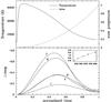 |
Fig. 5 Top: assumed temperature (solid line, left-hand scale) and emitting area (broken line, right-hand scale) evolution of a black body used in simulations of the brightness development of a flickering flare as a function of time. Bottom: calculated profiles of a simulated flickering flare in the bands of the UBVRI system. The inset shows the times of maxima (dots) as a function of the isophotal wavelength of the respective bands, together with a linear least-square fit (broken line). See text for details. |
The time development of the emitting area is taken to be
 .
This is based on the simple notion of a light source that expands linearly with time
(which may not necessarily be realistic!). With respect to the temperature evolution, good
results are obtained with a function that rises rapidly from low temperatures to a maximum
of just above 30 000 K and then gradually drops to about 6000 K at the end of the flare.
Both
(right-hand scale; normalized to a maximum value of 1; broken line) and Θ(t) (left-hand scale;
solid line) are shown as a function of time (the flare duration being normalized to
tfl =
1) in the upper frame of Fig. 5.
.
This is based on the simple notion of a light source that expands linearly with time
(which may not necessarily be realistic!). With respect to the temperature evolution, good
results are obtained with a function that rises rapidly from low temperatures to a maximum
of just above 30 000 K and then gradually drops to about 6000 K at the end of the flare.
Both
(right-hand scale; normalized to a maximum value of 1; broken line) and Θ(t) (left-hand scale;
solid line) are shown as a function of time (the flare duration being normalized to
tfl =
1) in the upper frame of Fig. 5.
With this choice of temperature and area evolution, and using the transmission functions of Bessell (1990), F(t) (i.e. the flare light curve) was calculated for the passbands of the UBVRI system. The constant was chosen such that F(t) obtains a maximum of F(t) = 1 in the U band. To mimic a constant background light, a quantity Fbg = 1 was added to all light curves before transforming them into magnitudes with an arbitrary zero point equal to the magnitude of the first point in the light curve corresponding to each passband. These light curves, depicting the magnitude development of the flare, are shown in the lower frame of Fig. 5.
The simulated flare has several characteristics in common with real flickering flares:
(i) Bruch (1992) found the mean ratio of the
gradients of the rise and decline of flickering flares in the B band of many light curves
(measured between the base and the peak of the flare) to be 1.18 ± 0.07, meaning that on average the
rise is slightly more rapid than the decline. In the simulated flare a very similar
gradient ratio of 1.21 is measured. But note that this value depends quite strongly on the
choice of Θ(t) and .
(ii) The amplitude of the flare is highest in the U band and declines
monotonically in longer wavelength bands6. This
agrees with observations. However, it is more difficult to make a quantitative assessment
here because the amplitude depends on the amount of the constant background light, which
was (unrealistically) assumed to be the same in all passbands in the current simulations.
(iii) There is a clear dependence of the time of maximum on the passband. This is shown in
the inset in the lower frame of Fig. 5, where the
maximum times (dots) are plotted as a function of the isophotal wavelength of the
photometric band. The broken line is a linear least-squares fit to the data. Thus, there
is a time lag of the flickering observed at different wavelengths. The least-squares fit
yields dΔTmax/
dλ = 1.4 × 10⁻⁵ time units/Å. To estimate
tfl , the average width σ of a Gauss fit to the
central peak of the auto-correlation function of the B band of the light curves
of TT Ari used to derive the results quoted in Sect. 4.2 was measured: σ
= 145 s ± 23 s. Taking this as the typcial flare duration (i.e.
tfl ≡
σ), dΔTmax/ dλ = 2.1 ×
10-3 s/Å. This is of the same order of magnitude as the
observed time lag for TT Ari (Table 3).
Thus, the simple scenario explored here can explain important characteristics of the flickering, in particular the main result of the present study, namely the observed time lag of the flickering at different optical wavelengths. The numerical value of dΔTmax/ dλ is of the same order of magnitude as that measured in real light curves and depends on the choice of the temperature and emission area evolution. Although not investigated here, it may be expected that deviations from black-body radiation have similar effects.
The results of this exercise hold for a single flare. But what about an entire light curve composed of many flares? If flickering were to consist of the additive superposition of many independent flares, it would be easy to construct such a light curve and investigate its properties. However, there are strong indications in CVs (e.g. Scaringi et al. 2012b) and even more so in X-ray binaries (e.g. Uttley et al. 2005) that flickering is the result not of an additive, but of a multiplicative process. The origins of disturbances in CV system that gives rise to flickering are largely speculative, and the physical mechanisms of how they lead to the emission of optical radiation are unknown. Therefore, the properties of an ensemble of (nonlinearly) superposed flares are not straightforward to predict, and I refrain from investigating this issue further.
5.2. Fireballs and the case of SS Cyg
The heuristic model discussed in the previous subsection can obviously not substitute a physical model for flickering flares. It was meant to show that parameter combinations for a light source exist that can plausibly explain the observed time lag of the flickering as a function of wavelength. The evolution of the (black body) temperature and the emitting area during the flare event was adjusted such that the flicker shape resembles that observed in real light curves.
A more sophisticated model must take into account the physical conditions in the flare light source. An interesting attempt in this direction has been published by Pearson et al. (2005). They modelled the light source as a fireball, that is, a hot, spherically symmetric expanding ball of gas, and calculated the emitting spectrum as a function of the input parameters and of time, permitting them to construct light curves at various wavelengths. They compared the results with light curves (time resolution: 2 s) in six bands between 3590 Å and 7550 Å of a particular flare extracted from high-speed spectro-photometric observations of the dwarf nova SS Cyg. Adjusting the model parameters such that the observed light curves are well fitted yields encouraging results if the fireball is assumed to be in isothermal expansion.
To investigate how the results of Pearson et al. (2005) fit in with the present study, I extracted the light curves of SS Cyg (consisting just of a single flare) from their Fig. 14. For convenience, the one corresponding to the band centred on 4545 Å is shown in the left panel of Fig. 6. In the same way as has been done for the other systems investigated in this study, the light curves of SS Cyg were cross-correlated, using the one centred on 4225 Å as reference. The time lag ΔTmax with respect to the reference band is shown as a function of wavelength in the right panel of Fig. 6 (filled circles). The wavelength of the reference band is marked by a cross.
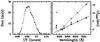 |
Fig. 6 Left frame: a flickering flare of SS Cyg centred on 4545 Å on 1998, July 8, as observed by Pearson et al. (2005). Right frame: ΔTmax as a function of wavelength of the comparison band for the observational data (filled circles) and the preferred fireball model (open circles). The solid and broken lines represent a linear least-squares fit to the data points (shortest wavelength point excluded). The location of the reference band is indicated by a cross. The dots with error bars are the average ΔTmax values of SS Cyg taken from Table 1, with the triangle representing the location of the respective reference band. |
For comparison, the average ΔTmax values for SS Cyg from Table 1 are shown in the figure as small dots with error bars (mean errors of the mean). The triangle indicates the location of the respective reference band. Unfortunately, Table 1 only contains data of SS Cyg taken in the UBV system, defining thus but two points in the diagram. Therefore, no strong conclusions can be drawn from the comparison with the results extracted from Fig. 14 of Pearson et al. (2005). However, both data sets appear to be roughly compatible with each other.
Except for the shortest wavelength band centred on 3615 Å, the data points from Pearson et al. (2005) follow a linear relationship (solid line) with an inclination of (2.3 ± 0.1) × 10-3 s/Å. This is very similar to the behaviour of V603 Aql, TT Ari, and RS Oph (Table 3 and Fig. 4).
I also determined the times of maximum light of the preferred model of Pearson et al. (2005) by fitting a high-order polynomial to the peak of the model curves extracted from their Fig. 14. The corresponding ΔTmax values are shown as open circles in Fig. 6. They follow a linear relationship (disregarding the data point at 3615 Å; broken line) with an inclination of (4.86 ± 0.01) × 10-3 s/Å. This is twice the value found for the observational data, indicating a slight disagreement between model and observations.
Although the fireball model is thus quite attractive to explain the time lag of the flickering as a function of wavelength, a vexing question remains: why does the data point at Pearson et al.’s (2005) 3615 Å band deviate from the linear relationship between ΔTmax and λ? Or, more generally, how can the tendency for a deviation from such a relationship at wavelengths shorter than the Balmer limit (Fig. 3) be explained? This can be due to optical-depth effects in the flaring light source. Pearson et al. (2005) found that their fireball is initially dominated by flux coming from optically thick regions. This changes in the course of its evolution, so that at late times, optically thin emission dominates. Thus, more Balmer continuum emission can escape from the light source at later phases, strengthening the flare at ultraviolet wavelengths and reversing the ΔTmax – λ relationship observed at longer wavelengths. The balance between optically thick and thin radiation will depend on the detailed structure of the fireball. Therefore, the late dominance of the Balmer continuum emission may be seen in some, but not all cases, explaining the different behaviour of the flickering time lag at very short wavelength in individual systems (e.g. V603 Aql and TT Ari vs. RS Oph and SS Cyg).
5.3. Alternative scenarios
Scaringi et al. (2013) sought to explain the time lags along lines different from fireballs (Sect. 5.2) or an evolving black-body-like light source, as investigated in Sect. 5.1. They discarded explanations in the context of models of flickering caused by the inward propagation of perturbations within the accretions disk (see e.g. Lyubarskii 1997; Pavlidou et al. 2001; Kotov et al. 2001; and Arévalo & Uttley 2006, for detailed models of this kind for X-ray binaries and galactic nuclei, and Yonehara et al. 1997; Dobrotka et al. 2010; and Scaringi 2014 for CVs), which assume that the observed optical variations are directly related to the inward propagation of matter in the accretion disk because then flickering variations in the blue should lag those in the red. This is contrary to what is observed. They also rejected a scenario of (practically) instantaneous reprocessing of light of a variable continuum source close to the centre of the accretion disk by some structure farther out. The time lag should then basically be equal to the light travel time. However, the typical dimensions of CVs are such that only the smallest observed time lags would not exceed the light travel time from the centre to the periphery of the disk. Moreover, the emission at long wavelengths should then be dominated by reprocessed light, which may not be likely.
If, however, reprocessing does not occur instantaneously, but on the local thermal time scale Scaringi et al. (2013) are able to qualitatively reconcile the observed time lags with reprocessing sites not too far out, provided that only the surface layer of the accretion disk reprocesses photons from the variable light source. As a final scenario, Scaringi et al. (2013) mentioned reverse shocks in the accretions disk (Krauland et al. 2013) that may originated in the boundary layer and deposit energy first in the hotter inner parts of the disk and then in the cooler outer regions.
None of scenarios mentioned in the previous paragraph is backed by a more detailed physical model. Therefore, it is hard to say if they lead to time scales compatible with the observed lags and are in accordance with other characteristics of the flickering such as, for example, the temporal and spectral development of individual flares. But it would be premature to discard them before an attempt has been made to predict the implied emission properties in some detail and to compare them with observations. It appears that the fireball model is at present the only physical model that has been advanced to a stage where definite predictions can be made about at least some flickering properties and that realistic parameter combinations can be found such that these predictions comply with observations. It must be recognized, however, that the model does not explain what makes the fireball explode in the first place. Moreover, it is not known to which degree a (linear or nonlinear) superposition of individual fireball events can reproduce the statistical properties of observed flickering light curves. Thus, it is by no means clear, which of the mentioned scenarios, if any, is realized in nature.
6. Conclusions
Confirming earlier results of Scaringi et al. (2013), it has been shown conclusively in the present study that flickering in cataclysmic variables does not occur exactly simultaneously in different photometric bands across the optical range. Instead, there is a time delay in the sense that individual events of the flickering develop slightly later at red than at blue wavelengths. In many of the investigated CVs, this effect can only be seen statistically in the ensemble of the available data because most of the light curves used are not of sufficient quality to resolve the time delay well enough in particular data sets. However, in the systems with the best data, V603 Aql and TT Ari, the effect can convincingly be measured individually. This is also true for RS Oph and SS Cyg. To these systems MV Lyr and LU Cam, observed by Scaringi et al. (2013), can be added.
The time lag of the flickering as a function of wavelengths is of the order of a couple of milliseconds per Ångstrom. The exact value may depend on the particular system, but appears not to change much within the same star on time scales of several years (i.e. the period spanned by the observational data; this does, of course, not preclude time lag changes when systems like TT Ari go into a low state).
The observed effect can be explained if the evolution of the radiation characteristics of the light source(s) responsible for the flickering is such that individual flares reach their peak emission slightly earlier at blue than at red wavelengths. It is not difficult to construct simple scenarios that are able to reproduce the observed time lag not only qualitatively, but also quantitatively, and which also agree with other properties that are generally observed in the flickering. While such scenarios lead to the observed effects, they can by no means substitute a realistic physical mechanism. The fireball model of Pearson et al. (2005) is most advanced when it comes to the actual radiation emission process that may be seen as flickering. It can reasonably well reproduce a flickering flare observed in SS Cyg in various wavelengths ranges not only with respect to the wavelength dependent time lag, but also with respect to the spectral and temporal development. However, the detailed emission processes implied in the context of other scenarios deserve to be investigated as well. This hold true especially for models where, contrary to the fireball model, a better understanding of the origin of underlying disturbance exists, for instance, the fluctuating disk model. It may be interesting to investigate whether the basic fireball radiation physics can be applied to these models as well.
One of the light curves of AE Aqr was observed only in U, V and R. In this case, the shortest wavelength band served as reference.
Weighting alternatively the data points according to the number of contributing light curves changes this value only slightly to (2.1 ± 0.4) × 10-3 s/Å.
In RS Oph the scatter of dΔTmax/ dλ of individual light curves is larger than in V603 Aql and TT Ari, which may be due to the inferior quality of the available data.
Even the extreme case where the flares are triangular in the reference band and saw-tooth-shaped in the comparison band (setting the rising branch of the original triangle to zero) only introduced a very slight asymmetry (but changed the location of the maximum significantly).
I chose the symbol Θ for the temperature to avoid confusion with the symbol T that is used in the quantity ΔTmax introduced earlier for the time lag of the flickering in different bands.
The similarity of the amplitudes in V and R is a consequence of the significantly larger width of the R passband.
Acknowledgments
I am deeply indebted to all those colleagues who put their light cuves of cataclysmic variables at my disposal. For the current study I used data contributed by N. Beskrovanaya, A. Hollander, R. E. Nather, M. Niehues, T. Schimpke, and N. M. Shakovskoy. I am particularly grateful to R. E. Robinson and E.-H. Zhang for their excellent light curves observed in the Stiening system, which were decisive for the success of this work. I thank the referee, Simone Scaringi, for many critical comments that helped to improve this publication.
References
- Anzolin, G., Tamburini, F., de Martino, D., & Bianchini, A. 2010, A&A, 519, A69 [NASA ADS] [CrossRef] [EDP Sciences] [Google Scholar]
- Arévalo, P., & Uttley, P. 2006, MNRAS, 367, 801 [NASA ADS] [CrossRef] [Google Scholar]
- Bachev, R., Boeva, S., Georgiev, T., et al. 2011, Bulg. Astron. J., 16, 31 [Google Scholar]
- Balman, Ş., & Revnivtsev, M. 2012, A&A, 546, A112 [NASA ADS] [CrossRef] [EDP Sciences] [Google Scholar]
- Baptista, R., & Bortoletto, A. 2004, AJ, 128, 411 [NASA ADS] [CrossRef] [Google Scholar]
- Belloni, T., Psaltis, D., & van der Klis, M. 2002, ApJ, 572, 392 [NASA ADS] [CrossRef] [Google Scholar]
- Bennie, P. J., Hildich, R. W., & Horne, K. 1996, in Cataclysmic variables and related objects (Kluwer), eds. A. Evans, & J. H. Wood, 33 [Google Scholar]
- Bessell, M. S. 1990, PASP, 102, 1181 [NASA ADS] [CrossRef] [Google Scholar]
- Bruch, A. 1989, Habil. Thesis, Univ. Münster [Google Scholar]
- Bruch, A. 1991, Acta Astron., 41, 101 [NASA ADS] [Google Scholar]
- Bruch, A. 1992, A&A, 266, 237 [NASA ADS] [Google Scholar]
- Bruch, A. 1996, A&A, 312, 97 [NASA ADS] [Google Scholar]
- Bruch, A. 2000, A&A, 359, 998 [NASA ADS] [Google Scholar]
- de Ruiter, H. R., & Lub, J. 1986, A&AS, 63, 59 [NASA ADS] [Google Scholar]
- Dobrotka, A., Hric, L., Casares, J., et al. 2010, MNRAS, 402, 2567 [NASA ADS] [CrossRef] [Google Scholar]
- Dobrotka, A., Mineshige, S., & Ness, J.-U. 2014, MNRAS, 438, 1714 [NASA ADS] [CrossRef] [Google Scholar]
- Dobrotka, A., Mineshige, S., & Ness, J.-U. 2015, MNRAS, 447, 3162 [NASA ADS] [CrossRef] [Google Scholar]
- Fritz, T., & Bruch, A. 1998, A&A, 332, 586 [NASA ADS] [Google Scholar]
- Garcia, A., Sodré Jr., L.,Jablonski, F. J., & Terlevich, R. J. 1999, MNRAS, 309, 803 [NASA ADS] [CrossRef] [Google Scholar]
- Heil, L. M., & Vaughan, S. 2010, MNRAS, 405, L86 [NASA ADS] [CrossRef] [Google Scholar]
- Henize, K. G. 1949, AJ, 54, 89 [NASA ADS] [CrossRef] [Google Scholar]
- Herbst, W., & Shevchenko, V. S. 1999, AJ, 118, 1043 [NASA ADS] [CrossRef] [Google Scholar]
- Horne, K., & Stiening, R. F. 1985, MNRAS, 216, 933 [NASA ADS] [Google Scholar]
- Jablonski, F., Baptista, R., Barroso, J., et al. 1994, PASP, 106, 1172 [NASA ADS] [CrossRef] [Google Scholar]
- Jensen, K. A., Córdoba, F. A., Middleditch, J., et al. 1983, ApJ, 270, 211 [NASA ADS] [CrossRef] [Google Scholar]
- Johnson, H. L., Perkins, B., & Hiltner, W. A. 1954, ApJS, 1, 91 [NASA ADS] [CrossRef] [Google Scholar]
- Kenyon, S. J., Kolotilov, E. A., Ibragimov, M. A., & Mattei, J. A. 2000, ApJ, 531, 1028 [NASA ADS] [CrossRef] [Google Scholar]
- Kotov, O., Churazov, E., & Gilfanov, M. 2001, MNRAS, 327, 799 [NASA ADS] [CrossRef] [Google Scholar]
- Krauland, C. M., Drake, R. P., Kuranz, C. C., et al. 2013, ApJ, 762, L2 [NASA ADS] [CrossRef] [Google Scholar]
- Lenouvel, F., & Daguillon, J. 1954, Ann. Astrophys., 17, 416 [NASA ADS] [Google Scholar]
- Linnell, A. P. 1950, Harvard Circ. 455, 1 [Google Scholar]
- Lub, J., & Pel, J. W. 1977, A&A, 54, 137 [NASA ADS] [Google Scholar]
- Lyubarskii, Yu. E. 1997, MNRAS, 292, 679 [NASA ADS] [CrossRef] [Google Scholar]
- Lynden-Bell, D. 1969, Nature, 223, 16 [Google Scholar]
- Nowak, M. A., Wilms, J., & Dove, J. B. 1999, ApJ, 517, 355 [NASA ADS] [CrossRef] [Google Scholar]
- Pavlidou, V., Kuijpers, J., Vlahos, L., & Isliker, H. 2001, A&A, 372, 326 [NASA ADS] [CrossRef] [EDP Sciences] [Google Scholar]
- Pearson, K. J., Horne, K., & Skidmore, W. 2005, ApJ, 619, 999 [NASA ADS] [CrossRef] [Google Scholar]
- Pogson, N. R. 1857, MNRAS, 17, 200 [NASA ADS] [CrossRef] [Google Scholar]
- Scargle, J. D., Steiman-Cameron, T. Y., Young, K., et al. 1993, ApJ, 411, L91 [NASA ADS] [CrossRef] [Google Scholar]
- Scaringi, S. 2014, MNRAS, 438, 1233 [NASA ADS] [CrossRef] [Google Scholar]
- Scaringi, S., Körding, E., Uttley, P., et al. 2012a, MNRAS, 421, 2854 [NASA ADS] [CrossRef] [Google Scholar]
- Scaringi, S., Körding, E., Uttley, P., et al. 2012b, MNRAS, 427, 3396 [NASA ADS] [CrossRef] [Google Scholar]
- Scaringi, S., Körding, E., Groot, P. J., et al. 2013, MNRAS, 431, 2535 [NASA ADS] [CrossRef] [Google Scholar]
- Scaringi, S., Maccaroni, T. J., & Middleton, M. 2014, MNRAS, 445, 1031 [NASA ADS] [CrossRef] [Google Scholar]
- Schimpke, T. 1998, Ph.D. Thesis, Univ. Münster [Google Scholar]
- Szkody, P., & Margon, B. 1980, ApJ, 236, 862 [NASA ADS] [CrossRef] [Google Scholar]
- Tamburini, F., de Martino, D., & Bianchini, A. 2009, A&A, 502, 1 [NASA ADS] [CrossRef] [EDP Sciences] [Google Scholar]
- Turner, H. H. 1907, MNRAS, 67, 316 [NASA ADS] [CrossRef] [Google Scholar]
- Uttley, P., & McHardy, I. M. 2001, MNRAS, 323, L26 [NASA ADS] [CrossRef] [Google Scholar]
- Uttley, P., & McHardy, I. M., & Vaughan, S. 2005, MNRAS, 359, 345 [NASA ADS] [CrossRef] [Google Scholar]
- van der Klis, M. 2004, ArXiv e-prints [arXiv:astro-ph/0410551] [Google Scholar]
- Vaughan, B. R., & Nowak, M. A. 1997, ApJ, 474, L43 [NASA ADS] [CrossRef] [Google Scholar]
- Walker, M. F. 1957, in Non-stable stars, ed. G. H. Herbig, Proc. IAU Coll., 3, 46 [Google Scholar]
- Walker, M. F., & Herbig, G. H. 1954, ApJ, 120, 278 [NASA ADS] [CrossRef] [Google Scholar]
- Walraven, T., & Walraven, J. H. 1960, Bull. Astr. Inst. Neth., 15, 67 [NASA ADS] [Google Scholar]
- Welsh, W. F., Wood, J. H., & Horne, K. 1996, in Cataclysmic variables and related objects (Dordrecht: Kluwer Academic), eds. A. Evans, & J. H. Wood, 29 [Google Scholar]
- Yonehara, A., Mineshige, S., & Welsh, W. F. 1997, ApJ, 486, 388 [NASA ADS] [CrossRef] [Google Scholar]
All Tables
All Figures
|
Fig. 1 Example of a light curve and the CCF of the brightness variations in two photometric bands. Top: B band light curve of V603 Aql observed on 1983 July 18. The solid line is a fit of a high-order polynomial to the data. Centre: residuals between the original light curve and the polynomial fit. Bottom left: CCF of the light curve shown in the top panel with the simultaneously observed light curve in the U band (broken line) and of the residuals between the original data and the polynomial fit (solid line). Bottom right: enlarged section of the maximum of the CCF shown as a solid line in the lower left panel (dots) together with a fit of a high-order polynomial to the data (broken curve). The broken vertical line indicates the location of the maximum of the fitted polynomial. |
| In the text | |
|
Fig. 2 Top: artificial flickering light curve used to estimate the accuracy
of the determination of flickering time lags. Bottom left: dependence
of ΔTmax on the noise level.
Bottom right: expected error of ΔTmax as a
function of the time resolution of the light curve for low
(0 |
| In the text | |
|
Fig. 3 Left: average ΔTmax for all investigated CVs as a function of isophotal wavelength of the comparison band. Right: average ΔTmax of all individual light curves, weighted in proportion to their duration. The broken line is a linear least-squares fit to the data points (excluding the points referring to the W and U bands), weighted by the inverse of their standard deviations. The error bars represent the mean error of the mean. In both frames the location of the reference band (B) is indicated by a cross. |
| In the text | |
|
Fig. 4 Average ΔTmax derived from high time resolution light curves of V603 Aql, TT Ari and RS Oph as a function of isophotal wavelength of the comparison band. The broken lines are linear least-squares fits to the data points (in the case of RS Oph without considering the points referring to the W and U bands), weighted by the inverse of their standard deviations. The location of the reference band (B) is indicated by a cross. The error bars represent the mean error of the mean. |
| In the text | |
|
Fig. 5 Top: assumed temperature (solid line, left-hand scale) and emitting area (broken line, right-hand scale) evolution of a black body used in simulations of the brightness development of a flickering flare as a function of time. Bottom: calculated profiles of a simulated flickering flare in the bands of the UBVRI system. The inset shows the times of maxima (dots) as a function of the isophotal wavelength of the respective bands, together with a linear least-square fit (broken line). See text for details. |
| In the text | |
|
Fig. 6 Left frame: a flickering flare of SS Cyg centred on 4545 Å on 1998, July 8, as observed by Pearson et al. (2005). Right frame: ΔTmax as a function of wavelength of the comparison band for the observational data (filled circles) and the preferred fireball model (open circles). The solid and broken lines represent a linear least-squares fit to the data points (shortest wavelength point excluded). The location of the reference band is indicated by a cross. The dots with error bars are the average ΔTmax values of SS Cyg taken from Table 1, with the triangle representing the location of the respective reference band. |
| In the text | |
Current usage metrics show cumulative count of Article Views (full-text article views including HTML views, PDF and ePub downloads, according to the available data) and Abstracts Views on Vision4Press platform.
Data correspond to usage on the plateform after 2015. The current usage metrics is available 48-96 hours after online publication and is updated daily on week days.
Initial download of the metrics may take a while.