| Issue |
A&A
Volume 579, July 2015
|
|
|---|---|---|
| Article Number | A23 | |
| Number of page(s) | 11 | |
| Section | Interstellar and circumstellar matter | |
| DOI | https://doi.org/10.1051/0004-6361/201425317 | |
| Published online | 19 June 2015 | |
Molecule sublimation as a tracer of protostellar accretion
Evidence for accretion bursts from high angular resolution C18O images
1 Centre for Star and Planet Formation, Niels Bohr Institute & Natural History Museum of Denmark, University of Copenhagen, Øster Voldgade 5–7, 1350 Copenhagen K., Denmark
e-mail: This email address is being protected from spambots. You need JavaScript enabled to view it.
2 European Southern Observatory, Karl-Schwarzschild-Str. 2, 85748 Garching, Germany
3 Institute for Astronomy, University of Hawaii at Manoa, Honolulu, HI 96822, USA
4 Department of Astronomy, University of Michigan, 1085 S. University Ave, Ann Arbor, MI 48109-1107, USA
Received: 11 November 2014
Accepted: 12 April 2015
Abstract
Context. The accretion histories of embedded protostars are an integral part of descriptions of their physical and chemical evolution. In particular, we want to know whether the accretion rates smoothly decline from earlier to later stages or whether they are in fact characterized by variations such as intermittent bursts.
Aims. We aim to characterize the impact of possible accretion variations for a sample of embedded protostars by measuring the sizes of the inner regions of their envelopes where CO is sublimated and relate these extents to the temperature profiles dictated by the current luminosities of the protostars.
Methods. Using observations from the Submillimeter Array we measure the extent of the emission from the C18O isotopologue toward 16 deeply embedded protostars. We compare these measurements to the predicted extent of the emission given the current luminosities of the sources through dust and line radiative transfer calculations.
Results. Eight out of sixteen sources show more extended C18O emission than predicted by the models. The modeling shows that the likely culprit for these signatures is sublimation due to increases in luminosities of the sources by about a factor of five or more during the recent 10 000 yr, i.e., the time it takes for CO to freeze-out again on dust grains. For four of these sources the increase must have been a factor of 10 or more. The compact emission seen toward the other half of the sample suggests that C18O only sublimates when the temperature exceeds 30 K – as expected if CO is mixed with H2O in the grain ice-mantles.
Conclusions. The results from this survey suggest that protostars undergo significant bursts about once every 20 000 yr, although the statistics suffer from the small sample size. The results illustrate the importance of taking the physical evolutionary histories into account for descriptions of the chemical structures of embedded protostars.
Key words: stars: formation / ISM: molecules / submillimeter: ISM / astrochemistry / protoplanetary disks / circumstellar matter
© ESO, 2015
1. Introduction
In their earliest stages, solar-type protostars are characterized by large amounts of cold gas and dust surrounding them. As the young star begins to heat up and accretion proceeds, this envelope is dissipated revealing the pre-main-sequence star surrounded by a circumstellar disk. Studies of young stars during the embedded stages are of prime importance for our understanding of their formation and early physical and chemical evolution: this is the phase when the star accretes the bulk of its mass and a circumstellar disk is formed. The physical and chemical structure of this disk possibly sets the initial conditions for subsequent planet formation. One of the important questions for our theories of formation of stars is how accretion proceeds: does it take place at a relatively constant rate throughout the protostellar evolution or does it strongly vary, for example as a result of the formation of the disk and possible fragmentation within it? Indirect evidence suggests that the accretion rates may vary through the protostars’ early years; for example, observations of outflows show in some cases clear knots or bullets that can be attributed to changes in the underlying accretion rates (e.g., Reipurth 1989; Arce et al. 2013). This paper presents maps of the C18O emission on scales of a few hundred to 1000 AU toward the dense envelopes of a sample of 16 embedded protostars with the Submillimeter Array (SMA). The aim of this work is to address whether possible variations in the protostellar accretion rates can be traced by their chemical signatures.
Strong luminosity bursts have for some time been recognized as one of the characteristics of young stars – at least during specific times of their pre-main-sequence phase where they may appear as FU Orionis objects at visible wavelengths (see, e.g., Audard et al. 2014, for a recent review). Such outbursts can be tied to the accretion onto and through the central protostellar disks and to possible instabilities in these disks (e.g., Bell & Lin 1994; Armitage et al. 2001; Vorobyov & Basu 2005; Zhu et al. 2009; Martin & Lubow 2011). Owing to the significant amounts of obscuring gas and dust, it is still unclear what happens in the earlier protostellar stages. Photometric comparisons of nearby star-forming regions at different epochs show small-scale luminosity variations on timescales ranging from days to years (e.g., Rebull et al. 2014) and are able to identify individual sources undergoing bursts in intervals of 5000–50 000 yr (Scholz et al. 2013). If these bursts are an indication that the accretion rates indeed also vary strongly, it would definitely be a critical aspect of the protostellar evolution.
In the earliest stages the luminosity of the protostar is thought to be dominated by the release of gravitational energy due to the accretion onto the central star (L ~ GM∗Ṁ/r∗). Generally, protostars are found to show a very broad luminosity distribution and be under-luminous compared to the expectation from constant infall toward the center of their natal cores (see, e.g., Kenyon et al. 1990 and Evans et al. 2009; as well as Dunham et al. 2014 for a recent review). This is another piece of evidence that has been taken in favor of episodic accretion during the earliest protostellar phases. In this picture, protostars spend most of their lifetimes in a low accretion rate mode, assembling material in the disk, and thus appear less luminous than expected based on accretion from their envelopes directly onto the central star. They could then accrete significant mass in relatively short bursts accompanied by increases in their luminosities that statistically would be relatively difficult to observe. However, because of the complex environments of young stars and possible continued infall onto and through the disk even during the more evolved stages, this picture may be too simplistic and the luminosity distribution itself may not offer a good constraint (e.g., Padoan et al. 2014).
In addition to the obvious important dynamical consequences of the exact protostellar accretion histories, they may also have important consequences on other aspects of the early evolution of protostars, for example, the chemical processes leading to the formation of larger molecules. This process involves a complex balance between molecules freezing out onto dust grains, grain-surface chemistry, and possible evaporation of the species before they are (re-)incorporated into ices in the circumstellar disks (see, e.g., Herbst & van Dishoeck 2009; Caselli & Ceccarelli 2012, for recent reviews). Variations in the accretion rates and consequently luminosities of the protostars will affect how long given molecules are present in solid or gaseous form and what the timescales are for the regulating chemical processes at different points during the protostellar evolution.
An interesting question is how these two issues – the accretion histories of protostars and corresponding luminosity evolution on the one hand and chemical evolution on the other – correspond. The strong dependence of the protostellar luminosity on the accretion rate will reflect directly on the thermal structure of the envelopes through the (almost instantaneous) heating of the dust (Johnstone et al. 2013). As these times are also characterized by freeze-out and sublimation of molecules that are strongly temperature dependent, clues may be found in the composition of ices and in the distributions of molecules in the gas- and solid-phase (e.g., Lee 2007; Poteet et al. 2013; Visser & Bergin 2012; Visser et al. 2015). One example of this is observations that show significant amounts of pure CO2 ices present around low to moderate luminosity protostars (Kim et al. 2012). The presence of pure CO2 ice is a good indication that significant thermal processing of the ices has taken place prior to the current evolutionary stage of the protostars. Even so, such observations of the total column density of a specific ice species only reveal the integrated history of the source and cannot be used as constraints on whether this distillation has taken place during the protostellar evolution or perhaps prior to the onset of collapse.
Another way of addressing this issue may be through resolved observations of the distributions of molecules in the environments. One possible example of this are ALMA observations of the deeply embedded protostar IRAS 15398–3359 (Jørgensen et al. 2013). The resolved images show a depression in the emission of H13CO+ in the inner 150–200 AU of the central protostellar core. One explanation for this depression is that HCO+ is destroyed by reactions with extended water vapor. However, the HCO+ depression is seen on the scales where the temperature is as low as 30 K given the current luminosity of the protostar – well below the temperature of 90–100 K needed for water to sublimate. A possibility is that the source has undergone a burst in accretion during the last 100–1000 yr, increasing the luminosity by up to a factor of 100 above what it currently is, causing water to sublimate on much larger scales. Ideally, one would use similar observations for many sources to constrain the prominence of such possible bursts: if such variations are indeed due to accretion variations, the distributions of even simpler species such as the optically thin isotopologues of CO may in fact already hold that information.
In this paper we present an analysis of C18O emission for a sample of 16 embedded protostars from previously published/archival SMA observations with the aim of revealing their CO emission distributions. The paper is laid out as follows. Section 2 describes the sample of sources and presents an overview of the observed images and spectra. Section 3 presents an analysis of the observed maps in contexts of detailed dust and line radiative transfer models – with a specific case study of the Class 0 protostar IRAS 03282+3035 setting up a more general analysis for the sample of 16 sources. The most important result, that half of these protostars in fact show more extended CO emission than what one should expect based on their current luminosities, is discussed in Sect. 4 along with the statistical implications of the frequency of bursts and the properties of the CO ices. Section 5 summarizes the main findings of the paper.
2. Data
As the basis for this analysis we constructed a sample of embedded protostars observed using the SMA (Ho et al. 2004). One of the preferred spectral setups for such observations at 230 GHz (1.3 mm) is a setting covering the J = 2−1 transitions of 12CO, 13CO, and C18O. For the purpose of this paper we focus on C18O, which typically shows centrally concentrated emission toward the location of the protostars. We utilized observations in the SMA’s compact-North and compact configurations that typically result in an angular resolution of 2–3′′ at these frequencies. Because of the interferometer’s lack of short-spacings, the observations are typically not sensitive to emission extended over scales larger than about 15′′.
The sample was put together utilizing the PROSAC study of Class 0 protostars (Jørgensen et al. 2007) as well as the sources from the SMA archive that were also used as a basis for the analysis of binarity by Chen et al. (2013). This sample comprises predominantly Class 0 objects with a few young Class I objects (i.e., sources with Tbol ≲ 150 K, or envelope masses of a few × 0.1 M⊙ to a few M⊙). We exclude sources with low signal-to-noise detections either because of their intrinsic C18O 2–1 line strengths or because of poorer data quality.
A few sources for which observations have not previously been presented were added. These include IRAS 03256-3055 observed on 2011 September 24 as part of a larger program to survey the population of young stars in the NGC 1333 cluster (PI: J. Williams) as well as observations of two intermediate mass protostars in Orion, MMS6 and MMS9 (Johnstone et al. 2003; Jørgensen et al. 2006b), from observations on 2007 February 7 (PI: J. Jørgensen). The full sample of sources is summarized in Table 1.
Sample of sources.
Both the archival data and the new observations were re-reduced using the MIR package (Qi 2012) and imaged and cleaned using Miriad (Sault et al. 1995). In the reduction we followed the standard procedures, calibrating the complex gains through observations of nearby quasars (typically two per track), passband calibration through observations of strong quasars before and/or after the observations, and flux calibrations utilizing planet observations. Continuum sensitivities (rms) in 2 GHz bandwidth for these observations were 0.5–1 mJy. Typically, the C18O 2–1 observations were performed by allocating 128–1024 channels to one of the (then) twenty-four 104 MHz chunks of the SMA correlator placed to cover the C18O transition. This resulted in spectral resolutions of 0.14–1.1 km s-1 with a typical line rms noise of 30–60 mJy beam-1 averaged over 1 km s-1 channels.
2.1. Overview of data
Figures 1 and 2 present overviews of the observed C18O 2–1 spectra and maps. The spectra were extracted in the beam toward the peak of the continuum emission for each source. The maps were made by integrating the emission over ± 1.5 km s-1 around the systemic velocity for each line.
The spectra show fairly regular profiles with little evidence of wings or other asymmetries as often is the case for the more common isotopologues and for larger scale single-dish maps. For the maps the emission is also relatively centrally condensed with low surface brightness extended emission in a few cases, but interestingly not for the most prominent outflow sources. Figure 2 also shows that for the sources with some structure in the C18O 2–1 emission there is no clear correlation with the outflow axis probed by 12CO 2–1. These observations likely reflect that the optically thin integrated C18O 2–1 emission is relatively little affected by the outflows present on larger scales, but is rather associated with the denser parts of the envelopes on scales ≲1000 AU; this is in agreement with what has been inferred from previous high angular resolution millimeter wavelength studies (e.g., Arce & Sargent 2006). In a few cases (e.g., IRAS 03256 and IRAS 15398) small offsets are seen between the continuum and line emission in Fig. 2: for these sources it is seen that the line emission is generally better aligned with location of the central heating source as traced by shorter wavelength (e.g., Spitzer data) and the SMA continuum emission is more strongly affected by the dust density and temperature distribution on the scales of the envelope-disk transition.
In the following we focus on reproducing the extent of the integrated emission from the C18O 2–1 transition, but further restrict the analysis beyond what is shown in Figs. 1 and 2 and do not include the most extended (low surface brightness) emission as justified below.
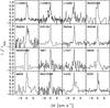 |
Fig. 1 C18O 2–1 spectra toward the peak of its integrated emission for each of the protostars in the sample. |
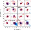 |
Fig. 2 Integrated C18O 2–1 emission for each of the protostars shown as contours on top of continuum maps of each source. The contours are shown at steps corresponding to 20%, 30%, 40%, etc., of the peak emission in the integrated line maps. The dashed lines indicate the outflow axis from SMA 12CO 2–1 maps for the sources where this line was observed simultaneously with C18O 2–1. |
3. Analysis
The main aspect of the analysis of the C18O 2–1 emission is to test whether its extent can be reproduced through simple radiative transfer models of the envelope structure and protostellar luminosities. We first present an in-depth analysis of a single source as a test case (Sect. 3.1) before considering the entire sample of sources in a general manner (Sect. 3.2).
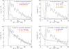 |
Fig. 3 Comparison between different parameterizations of the envelope physical and chemical structure (for details of the parameters for each model, see Table 2) comparing the observed and modeled visibility amplitude as function of projected baseline length for IRAS 03282. In each panel the observed integrated C18O emission is seen as datapoints with models as lines. The gray histogram indicates the expected amplitude for zero signal. In panel a) models with constant abundances and a luminosity corresponding to the current source luminosity (1.1 L⊙). In panel b) models with a changing abundance at the radius where the temperature increases above 20 K. In panel c) the source luminosity is increased and CO consequently sublimates at larger radii providing the variation in intensity as function of projected baselines required to fit the data. Finally panel d) tests the importance of varying the strength of the external interstellar radiation field – which again is found to only affect the outer parts of the envelopes. |
3.1. Test case: IRAS 03282+3035
As a test case we focus on the IRAS 03282+3035 Class 0 protostar (IRAS 03282 in the following): IRAS 03282 is a deeply embedded protostar in the Perseus molecular cloud driving a northwest-southeast oriented outflow seen in high resolution millimeter interferometric maps (e.g., Arce & Sargent 2006) and in mid-infrared images from the Spitzer Space Telescope (e.g., Jørgensen et al. 2006a). Its compact C18O 2–1 emission is particularly bright and regular, making it a good test case for the method.
To model the C18O 2–1 profile we construct a model for the envelope based on its submillimeter continuum and line emission that is similar to the approach adopted in, e.g., Jørgensen et al. (2002, 2009). We adopt a 1D power-law density profile for the envelope, ρ ∝ r− p, and calculate its temperature profile self-consistently based on the luminosity of the source. For the calculations we utilize the radiation transfer code Transphere1 that solves the 1D dust radiative transfer problem for absorption and re-emission following the methods described in Dullemond et al. (2002). The normalization of the envelope density profile is fixed by comparison to single-dish submillimeter continuum observations (for further discussion see, e.g., Jørgensen et al. 2009). In the following we test models that fix p at 1.5 (the expectation for a free-falling envelope) and 2.0 (corresponding to a static isothermal sphere). From radiative transfer models of submillimeter continuum brightness profiles from JCMT/SCUBA observations, p is typically found to vary between these values with uncertainties of ± 0.2 in the measurements for individual sources (e.g., Jørgensen et al. 2002; Shirley et al. 2002; Kristensen et al. 2012).
The resulting density and temperature profiles from the dust radiative transfer calculations are then used for line radiative transfer calculations using the Ratran code (Hogerheijde & van der Tak 2000). Adding the velocity field and an abundance profile for a given molecule, Ratran solves the full non-LTE radiation problem to estimate its level populations as a function of location and subsequently ray-traces the solution to calculate synthetic images that can be compared directly to the observations. For the CO abundance profile we adopt a simple step function (e.g., Jørgensen et al. 2005). We multiply the synthesized images with the interferometric primary beam and Fourier transform the images for the direct comparison to the observations in the (u,v)-plane. Figure 3 explores the influence of different models on the CO emission profiles. In the panels of this figure the data and models are represented by the amplitude of the integrated emission as function of projected baseline length.
With these choices the model has a number of free parameters: the envelope inner and outer radius, its density normalization, and the CO abundance profile as a function of radius. By restricting the comparison to specific baselines the inner and outer envelope radii are not important for the results and we adopt 25 AU and 8000 AU as in Jørgensen et al. (2009). The normalization of the density profile and the absolute abundances are naturally degenerate in the sense that a denser or more massive envelope can fit the data with a lower abundance. The shape of the abundance profile on these scales is critical, however.
Figure 3 compares the observed C18O visibility amplitudes to the predictions from a range of models summarized in Table 2. Figure 3a illustrates the simplest models where the C18O abundance is kept constant throughout the envelope at 2 × 10⁻⁷, corresponding to a canonical CO abundance of 10-4, and also shows models where the abundance is increased and decreased by a factor of 8. Two important conclusions can immediately be drawn from this plot. If the C18O abundance is constant at the canonical level, the emission of the 2–1 transition becomes optically thick throughout the envelope so that further increases in abundance do not change the brightness profiles significantly. For low abundances, the model underproduces both the emission on large scales (short baselines) and the single-dish observations. For all three models little emission is seen on long baselines compared to the observations that show significant emission out to baselines of approximately 35–40 kλ. This indicates that the abundance must change on small scales – rather than staying constant throughout the envelope – making the emission maps appear more centrally condensed.
Models with an abundance enhancement of CO by up to two orders of magnitude (Fig. 3b) at the radius where the temperature increases to either 20 or 30 K (corresponding to the CO sublimation temperature of pure or slightly mixed CO ice) do a slightly better job in the sense that they produce some emission at the smaller scales/longer baselines, but they are still not able to capture the full emission profiles. In addition, for a canonical CO abundance on small scales the model severely underproduces the emission on larger scales, so the change has to occur on larger scales than would be predicted given the current luminosities. The figure also includes a model with an abundance decreasing through the protostellar envelope from the outer edge toward the center until the point where the temperature reaches 20 K and then increases abruptly back to the canonical value. Such models could capture, for example, the gradual freeze-out with increasing densities (Jørgensen et al. 2005; Fuente et al. 2012) inferred on the basis of single-dish and lower resolution interferometric data. In addition, this model does not affect the emission on the longer baselines. Thus, the key point from this analysis is that the shape of the visibility amplitude curve as a function of projected baselines is not affected by the exact abundance structure on larger scales. The task is therefore to determine what luminosity is required to shift the CO sublimation temperature out to the radius where the enhancement is seen in the CO emission maps.
Measured and predicted extents of the deconvolved C18O emission – as well as the current luminosities and luminosity enhancements required to reproduce the extended C18O emission.
Figure 3c demonstrates three models that fit the data well. These represent models where the CO sublimates with an abundance enhancement within the radius where the temperature increases above 20 K in a ρ ∝ r-1.5 envelope around a 5 L⊙ protostar, as well as two models where CO sublimates at 30 K and the density profile has either p = 1.5 with a luminosity of 30 L⊙ or p = 2.0 and a luminosity of 50 L⊙. These models are indistinguishable at baselines longer than 15 kλ. Increasing or decreasing the luminosity by more than about 20% makes the fits significantly worse. These models illustrate some of the degeneracy between the best fit parameters and the limitations of this method: naturally there is a degeneracy between the temperature at which CO sublimates and the required luminosity enhancement, although this can be somewhat alleviated by considering the sample in its entirety. Likewise, the exact luminosity enhancement is dependent on the steepness of the density profile: a steeper density profile causes the C18O brightness profile to become steeper and thereby requires a larger enhancement in luminosity to shift the sublimation radius outward. In the following we continue to consider the case where p = 1.5, but we note that the required luminosity enhancement may be up to a factor of 2 larger for steeper density profiles (i.e., in that context the inferred enhancement is a lower limit). It is clear that as long as only the longer baselines are considered the structure and/or abundance on larger scales (shorter baselines) are unimportant for the fits. This point is further illustrated in Fig. 3d where the strength of the external interstellar radiation field rather than the internal luminosity of the source is varied; such models may vary the profiles on the large scales through the sublimation of the CO and may change the excitation temperature, but do not affect the shape of the emission profile in the inner 10′′ (baselines longer than 15 kλ) corresponding to radii ≲1000 AU for the studied sources.
In summary, for the test case of IRAS 03282 it is not possible to reproduce the observed C18O brightness profiles unless its abundance profile reflects sublimation at a temperature set by a higher luminosity of the source than its current ≈1 L⊙.
3.2. Sample approach
Inspired by the discussion above we define the approach for the entire sample of sources. For each source we derive the extent of the integrated C18O 2–1 emission by fitting 2D Gaussian profiles in the (u,v)-plane to limit systematics due to the deconvolution. We restrict the fit to baselines longer than 15 kλ (about 20 m; or scales corresponding to about 10′′). As shown above (Sect. 3.1) this selection is ideal for measuring the extent of the regions of the envelopes where CO sublimates and for filtering the remainder of the low surface brightness extended emission associated with the ambient cloud. Modeling the emission on shorter baselines can be used together with single-dish observations to probe the amount of CO in the larger scale envelope and, for example, the rate at which CO freezes-out or the importance of photo-desorption (e.g., Jørgensen et al. 2005; Fuente et al. 2012). However, as here we are mainly interested in the gradients in C18O emission associated with CO sublimating at higher temperatures and aim to treat all sources consistently, we focus only on the emission on the longer baselines. Table 3 lists the deconvolved extent of the C18O 2–1 emission (FWHM) for each source and Fig. 4 plots these values (as the radius = FWHM/2) versus the current luminosities of the sources. From this it can already be seen that there is no correlation between the deconvolved extents and the current luminosities of the protostars, which one would expect if the heating by the central protostar dominated the temperature profile and thus determined the size of the region where CO is in the gas-phase.
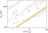 |
Fig. 4 Radii of C18O emission at the half-maximum intensity for the 16 Class 0 protostellar sources studied in this paper (symbols) as a function of luminosity compared to the predictions from radiative transfer models: the solid line indicates a 1 M⊙ envelope with sublimation of CO and resulting increase in abundance by two orders of magnitude within the radius where the temperature increases above 30 K. The shaded area corresponds to envelope masses ranging from 0.3−3 M⊙. The dotted line represents models where the sublimation takes place at a temperature of 20 K. Finally, the dashed lines correspond to sources where the luminosity has been increased by one and two orders of magnitude and the sublimation takes place for a temperature of 30 K. The typical uncertainties on the measured extents are 10–20% of the plotted values; the typical uncertainties in the predicted extents are up to 50% owing to the uncertainties in the underlying model, luminosity, etc. |
Figure 4 also shows the predictions for the C18O emission from a set of radiative transfer models. We do not construct models for each individual source, but rather make predictions of the C18O emission extent from a generic envelope model with ρ ∝ r-1.5 and ranges of luminosities. For each of these models we follow the same procedure as described in Sect. 3.1, performing the dust and line radiative transfer calculations and predicting the C18O 2–1 emission profile assuming that the CO comes off dust grains with a two orders of magnitude change in abundance for a sublimation temperature of 30 K (see the discussion of a possible lower sublimation temperature below). The models are processed in the same way described above, multiplied by the interferometric primary beam field of view and Fourier-transformed, and the resulting extent measured by fitting a 2D Gaussian profile in the (u,v)-plane. The model predictions are compared to the observational data in Fig. 4 with Table 3 providing the current luminosities, the predicted sizes of the CO emission profiles given these luminosities, the actual measured sizes, and the corresponding enhancements in luminosities. The uncertainty of the inferred value for the luminosity enhancement from the model fits is about 20% (Sect. 3.1). Owing to systematic uncertainties (e.g., due to the model assumptions such as the envelope mass in the general approach), variations should only be considered significant on a 50% or higher level, but generally considered lower limits because the method is insensitive to the most intense bursts due to the interferometer resolving out more extended emission and the degeneracy with the steepness of the envelope density profiles (Sect. 3.1).
A few things are immediately apparent from Fig. 4. The observed extents of the CO emission do not show a clear correlation with the current luminosities with typical variations in the deconvolved sizes for any given luminosity of about a factor of three, with the exception that no sources with high luminosities have very compact C18O 2–1 emission. If the extent of the C18O emission is determined primarily by the sublimation due to heating by the central protostar, this is unsurprising; however, as the sublimation is expected to be instantaneous compared to the evolutionary timescales of the protostars, it is unlikely to encounter such sources. It is indeed seen that the sources with the most compact emission for each luminosity nicely track the predictions from the radiative transfer models. In contrast, for about half the sources the CO emission is seen to be extended as one would expect if the luminosity were from a factor of about five up to two orders of magnitude higher than it is now. Under the same interpretation this is an indication that their current luminosities are not what determines the observed extent of the CO emission.
4. Discussion
4.1. Envelope mass and CO sublimation temperature
Two parameters that may affect the exact value of the inferred increase in luminosity on the basis of the CO extent are the assumed envelope mass and CO sublimation temperature in the generic models.
A simple test reveals that the former is of little importance for the solar-type protostars considered here. Figure 4 shows the spread in inferred CO sublimation radii for envelope masses varying by an order of magnitude from 0.3 to 3 M⊙: the variation in the predicted CO sublimation radii is about 10%. This reflects that the envelopes are largely optically thin to their own radiation, in which case the temperature profile can be described by a power-law temperature profile with a radius whose overall scaling is only determined by the luminosity of the source (e.g., Scoville & Kwan 1976; Doty & Leung 1994; Chandler & Richer 2000).
The adopted CO sublimation temperature is much more important as is also illustrated in Fig. 4. Shifting the sublimation temperature from 30 K to 20 K in the models shifts the radius to where CO evaporates out to align with the predictions for where it would be for a model with a sublimation temperature of 30 K but luminosities an order of magnitude higher.
This discussion is highly relevant: traditionally many studies of modeling sublimation of CO in star-forming regions adopt a binding energy of 855–960 K from laboratory experiments of pure CO (e.g., Sandford & Allamandola 1993; Bisschop et al. 2006). However, laboratory experiments also show that mixing the CO with H2O ice can increase the CO binding energy to ≈1200–1300 K (e.g., Collings et al. 2003; Noble et al. 2012). The thermal sublimation rate at a constant dust temperature, Td, depends exponentially on the binding energy, Eb, as ξ ∝ exp(Eb/Td) (e.g., Eq. (4) of Rodgers & Charnley 2003). For a binding energy of 960 K it takes less than one year for CO to sublimate for a dust temperture above 21 K. For a binding energy of 1300 K the sublimation rate slows down so that it takes less than one year for CO to sublimate only at temperatures above 28 K. Observationally, there is some evidence for a higher sublimation temperature based on modeling of multi-transition CO observations as well as previous high angular resolution observations (Jørgensen 2004; Jørgensen et al. 2005; Yıldız et al. 2013).
It is worth noting that half of the sources do in fact show compact CO emission that is well fit by the models with a sublimation temperature of 30 K adopting their current source luminosities. That directly argues against a lower sublimation temperature as it would result in more extended CO emission than observed. In contrast, a higher sublimation temperature cannot be ruled out based on the observations here, but it would imply that a larger fraction of the sources have experienced increases in luminosities in their recent histories.
This result is not necessarily a contradiction with some high resolution imaging studies of more evolved disks around T Tauri stars that may favor lower sublimation temperatures through indirect imaging (e.g., Qi et al. 2013; Mathews et al. 2013), although it might be interesting to revisit those studies and to use models adopting a higher binding energy/sublimation temperature. Whereas the CO and H2O ices are likely formed simultaneously in the protostellar environments where the temperatures generally are low, the ices in the disks around T Tauri stars may have undergone some heating and sublimation before reformation when entering the disks and the material cooling down. As the binding energy of H2O is much higher than that of CO, only a small fraction of the water may not sublimate before entering the disk (e.g., Visser et al. 2009; Cleeves et al. 2014). This would naturally lead to the formation of a clearer onion-shell structure of the ices in the disks with an inner layer of H2O ice and an outer layer of more purified CO ice with a resulting lower binding energy. It is possible that the CO sublimation temperature varies from source to source, e.g., depending on the water content in their ambient environment. This would naturally be an important result in itself, although no other direct observational evidence exists for such variations. In that case, one could only argue that three out of the sixteen sources would show evidence of enhanced luminosities in their recent histories.
In any case, this discussion emphasizes the need for high quality laboratory measurements of ices relevant for astrophysical environments, as well as a careful consideration of the exact conditions and chemical histories of the studied regions.
4.2. Ice sublimation as a tracer of accretion bursts
A fairly straightforward interpretation of the variations in the extent of the central C18O emission relative to the predictions given the current source luminosities is that the protostars in fact undergo bursts of accretion and corresponding luminosities. Figure 5 illustrates this progression through three characteristic phases: in a period of time before the burst, or equivalently a long time since the previous burst, the chemistry will set itself in a relatively steady state with CO frozen-out outside the radius where the temperature reaches the sublimation temperature and in the gas-phase within this (Stage 1 in Fig. 5). During the burst this radius will be shifted outward and due to the short timescale for sublimation of CO the freeze-out/sublimation boundary will shift outward correspondingly (Stage 2). For typical binding energies for CO (see Sect. 4.1) the timescale for CO to sublimate at temperatures of 30 K is on the order of minutes to days, i.e., much shorter than the typical dynamical timescales related to the infall of material from the envelope. Finally, after the burst has finished and the source reset to a low luminosity, CO will begin to freeze-out again. However, owing to the slower freeze-out it will still appear to be extended for a longer period of time (Stage 3).
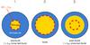 |
Fig. 5 Interpretation of the extended CO emission signatures due to variations in source luminosities. The dark blue and yellow regions indicate where CO is frozen out and in the gas-phase in three characteristic situations around a protostellar burst in luminosity. The red dashed line is the radius where the temperature in the envelope reaches the sublimation temperature for CO. The three panels indicate the situations (1) just before a burst where the CO sublimates out to a radius defined by the current luminosity of the protostar; (2) during a burst where the luminosity of the protostar increases and the CO sublimation radius moves outward; and (3) immediately after a burst where CO remains in the gas-phase in a large region and before it freezes-out again. |
It is possible to be more quantitative about the timescales. For a characteristic envelope with a mass of 0.3–0.5 M⊙, a size of 10 000 AU (radius), and a density profile dropping as ρ ∝ r-1.5, the timescale for CO to freeze-out at the density at 300–500 AU is on the order of tdep ~ 104 yr (e.g., Eq. (3) of Rodgers & Charnley 2003). Thus, if a given source undergoes an increase in luminosity, CO would stay in the gas-phase – and its emission appear extended – for this period of time after the luminosity has decreased again.
With additional assumptions one can even turn this into a statement about the frequencies of such bursts implied by the current data. One can for example assume that the duration of the burst in Stage 2 (t2) from Fig. 5 is much shorter than the total duration in Stages 1–3 (t1 + t2 + t3); based on the observed luminosity distributions of young stellar objects from the Spitzer Space Telescope c2d legacy program and simple calculations of the accretion rates, Evans et al. (2009) argued that half the final mass of a given young star is accreted during 7% of the duration of the embedded stages. Similarly, from a comparison between numerical hydrodynamical simulations of collapsing cores and the distributions populations of young stars, Dunham & Vorobyov (2012) argued that modeled protostars on average spend ≈1% of their lifetimes in modes of accretion bursts. The above analysis shows that half of the sources have CO extents corresponding to luminosities about a factor of five or more above the current. In the context of the scenario outlined above this would imply that t1 ≈ t3. As the duration of t3 by definition is the depletion time, tdep, this suggest that a given source undergoes a burst every t1 + t3 ~ 2tdep ≈ 20 000 yr – or approximately five bursts during the 105 yr duration of the deeply embedded Class 0 stage. If, on the other hand, one assumes that variations in the CO sublimation temperatures between the different sources is the dominant reason for the variations in the CO extent and thus that only three out of the sixteen sources show significant C18O 2−1 extents, this would imply a burst every 50 000 yr. These timescales are in good agreement with estimates by Scholz et al. (2013) who compared Spitzer and WISE photometric data for young stars in nearby star-forming regions and identified 1–4 bursts in a sample of 4000 young stars. Translated into frequencies these numbers would correspond to bursts in intervals of about 5000 and 50 000 yr.
It is worth re-emphasizing the reasons why the method outlined in this paper is useful. First and foremost the C18O emission is not significantly affected by outflows or the ambient environment, for example. This is observationally shown given the narrow lines and relatively centrally condensed distributions of the line emission. This is mainly a result of the C18O being largely optically thin and thus predominantly sensitive to the high column densities of material associated with the protostars themselves. An analysis of the chemistry of common molecular tracers during and after the accretion burst is presented by Visser et al. (2015). In addition, any more smoothly distributed material on larger scales in the clouds is filtered by the interferometer. Secondly, the timescales for sublimation and freeze-out of the CO molecule are apparently well matched for its use as a tracer. Observationally, the typical envelope masses (and consequently densities) change on timescales of a few 105 yr from one to a few M⊙ to 0.1 to 0.5 M⊙ for early Class I sources, which is still sufficiently long for freeze-out and sublimation to occur. In fact, the observation that some sources do show the compact C18O emission directly shows that large variations on short timescales are unlikely. Had the frequency of bursts been higher than 1 /tdep, the sources would never have returned to Stage 1, but instead would have cycled between Stages 2 and 3 – with the result that the CO emission would always appear extended.
Of course these estimates are still rather crude owing to the small sample size. In addition, owing to the inherent uncertainties in the modeling discussed above, the analysis does not constrain the strengths of the bursts. For example, owing to the low sublimation temperatures, the CO isotopologues are not sensitive to very intense bursts that may cause it to evaporate out to the largest scales probed by the interferometric data (~1000 AU radius). Observations of other species that sublimate at higher temperatures (or species reacting to these temperatures) could help refine the accretion histories of protostars. Observations of the H2O could for example be used to directly test whether the binding energy of CO varies significantly from source to source: if the extents of the H2O emission is found to vary in conjunction with CO, it would indicate that luminosity variations dominate over variations in the binding energy. Surveys of larger unbiased samples of sources coupled to models would also greatly improve the statistics on smaller scales and/or correlate for example to physical properties of the ambient environment or the physical structure of the protostars on small-scales that may drive possible accretion variations. A more detailed description of the dynamical evolution of the protostellar envelopes on the characteristic 104 yr timescale for freeze-out would also be needed to refine the statistics. Finally, although the maps do not show any indications that the C18O 2–1 emission is affected by the presence of outflows, sensitive high angular resolution observations will be needed to quantify what impact outflows have on the quiescent gas and how they contribute to shaping the envelopes.
Turning the argument around: results such as these emphasize the need to take the accretion histories of embedded protostars into account when considering their chemistry. If similar accretion variations can be confirmed to take place during the evolution of embedded protostars, they may have profound implications for the gas-grain chemistry interplay taking place during the early stages of protostellar evolution.
5. Summary
An analysis of maps of C18O J = 2–1 emission from the Submillimeter Array (SMA) toward a sample of deeply embedded protostars has been presented. The maps trace the distribution of C18O in the envelope on few hundred to thousand AU scales. The maps are compared to detailed continuum and line radiation transfer models, in particular the predictions for the extent of the CO emission given the current luminosities of the sources. The conclusions are as follows:
-
The C18O spectra appear relatively symmetric with little evidence of strong outflow action. The integrated emission maps are likewise regular with only faint low surface brightness extended emission. These results indicate that the integrated C18O emission is predominantly picking up the material in the denser parts of the envelopes on ≲1000 AU scales.
A case study of the IRAS 03282 protostar is used to demonstrate a method in which the deconvolved extent of the C18O emission measured in the (u,v)-plane can be compared to radiation transfer models for the protostellar envelope. The key parameter in this comparison is the assumed luminosity of the source and consequently the radius at which CO sublimates at temperatures of 20–30 K. This dominates over other effects such as the envelope’s physical structure and exact absolute abundances.
In the comparison of the entire sample it is found that half of the sources show C18O line emission that is more extended than predicted by models based on the current luminosities of the sources if CO sublimates at temperatures of 30 K. For those sources the increase must have been more than about a factor of five; for four of these the inferred luminosity would be more than a factor of 10 higher.
A CO sublimation temperature lower than 30 K cannot be reconciled with the observations of half the sources with compact emission. The sublimation temperature of 30 K in these environments may be taken as evidence of a higher binding energy for the CO than is expected for pure ices, which is a possibility if CO is mixed in with CO2 and/or H2O.
The half of the sources in the sample that show more extended C18O emission are the candidates that have undergone a recent change in luminosity, e.g., owing to a burst in accretion rate. This would have taken place within the last ~104 yr, which is the time it takes for CO to freeze-out on dust grains at the densities characteristic of the 300−500 AU radii of the protostellar envelopes observed here. If such bursts of accretion are taking place in general, this survey would imply that a protostar undergoes approximately 5 bursts during its first 105 yr. If one assumes that the CO sublimation temperature varies between 20 and 30 K from source to source, a conservative estimate would be an interval of 50 000 yr between the bursts.
Acknowledgments
We thank the referee for a thorough report that greatly helped the presentation and discussion of the results. This paper is based on data from the Submillimeter Array: the Submillimeter Array is a joint project between the Smithsonian Astrophysical Observatory and the Academia Sinica Institute of Astronomy and Astrophysics and is funded by the Smithsonian Institution and the Academia Sinica. The research of J.K.J. was supported by a Junior Group Leader Fellowship from the Lundbeck foundation. Research at Centre for Star and Planet Formation is funded by the Danish National Research Foundation and the University of Copenhagen’s programme of excellence.
References
- Arce, H. G., & Sargent, A. I. 2006, ApJ, 646, 1070 [NASA ADS] [CrossRef] [Google Scholar]
- Arce, H. G., Mardones, D., Corder, S. A., et al. 2013, ApJ, 774, 39 [CrossRef] [Google Scholar]
- Armitage, P. J., Livio, M., & Pringle, J. E. 2001, MNRAS, 324, 705 [NASA ADS] [CrossRef] [Google Scholar]
- Audard, M., Ábrahám, P., Dunham, M. M., et al. 2014, Protostars and Planets VI, eds. H. Beuther, R. S. Klessen, C. P. Dullemond, & Th. Henning (Tucson: University of Arizona Press) [Google Scholar]
- Bell, K. R., & Lin, D. N. C. 1994, ApJ, 427, 987 [NASA ADS] [CrossRef] [Google Scholar]
- Billot, N., Morales-Calderón, M., Stauffer, J. R., Megeath, S. T., & Whitney, B. 2012, ApJ, 753, L35 [NASA ADS] [CrossRef] [Google Scholar]
- Bisschop, S. E., Fraser, H. J., Öberg, K. I., van Dishoeck, E. F., & Schlemmer, S. 2006, A&A, 449, 1297 [NASA ADS] [CrossRef] [EDP Sciences] [Google Scholar]
- Black, J. H. 1994, in The First Symposium on the Infrared Cirrus and Diffuse Interstellar Clouds, eds. R. M. Cutri, & W. B. Latter, ASP Conf. Ser., 58, 355 [Google Scholar]
- Caselli, P., & Ceccarelli, C. 2012, A&ARv, 20, 56 [NASA ADS] [CrossRef] [MathSciNet] [Google Scholar]
- Chandler, C. J., & Richer, J. S. 2000, ApJ, 530, 851 [NASA ADS] [CrossRef] [Google Scholar]
- Chen, X., Arce, H. G., Zhang, Q., et al. 2013, ApJ, 768, 110 [NASA ADS] [CrossRef] [Google Scholar]
- Cleeves, L. I., Bergin, E. A., Alexander, C. M. O. D., et al. 2014, Science, 345, 1590 [NASA ADS] [CrossRef] [Google Scholar]
- Collings, M. P., Dever, J. W., Fraser, H. J., McCoustra, M. R. S., & Williams, D. A. 2003, ApJ, 583, 1058 [NASA ADS] [CrossRef] [Google Scholar]
- Doty, S. D., & Leung, C. M. 1994, ApJ, 424, 729 [NASA ADS] [CrossRef] [Google Scholar]
- Dullemond, C. P., van Zadelhoff, G. J., & Natta, A. 2002, A&A, 389, 464 [NASA ADS] [CrossRef] [EDP Sciences] [Google Scholar]
- Dunham, M. M., & Vorobyov, E. I. 2012, ApJ, 747, 52 [NASA ADS] [CrossRef] [Google Scholar]
- Dunham, M. M., Crapsi, A., Evans, II, N. J., et al. 2008, ApJS, 179, 249 [NASA ADS] [CrossRef] [Google Scholar]
- Dunham, M. M., Stutz, A. M., Allen, L. E., et al. 2014, in Protostars and Planets VI, eds. H. Beuther, R. S. Klessen, C. P. Dullemond, & T. Henning (Tucson: University of Arizona Press), 914, 195 [Google Scholar]
- Evans, N. J., Dunham, M. M., Jørgensen, J. K., et al. 2009, ApJS, 181, 321 [NASA ADS] [CrossRef] [Google Scholar]
- Fuente, A., Caselli, P., McCoey, C., et al. 2012, A&A, 540, A75 [NASA ADS] [CrossRef] [EDP Sciences] [Google Scholar]
- Green, J. D., Evans, II, N. J., Jørgensen, J. K., et al. 2013, ApJ, 770, 123 [NASA ADS] [CrossRef] [Google Scholar]
- Herbst, E., & van Dishoeck, E. F. 2009, ARA&A, 47, 427 [NASA ADS] [CrossRef] [Google Scholar]
- Ho, P. T. P., Moran, J. M., & Lo, K. Y. 2004, ApJ, 616, L1 [NASA ADS] [CrossRef] [Google Scholar]
- Hogerheijde, M. R., & van der Tak, F. F. S. 2000, A&A, 362, 697 [NASA ADS] [Google Scholar]
- Johnstone, D., Boonman, A. M. S., & van Dishoeck, E. F. 2003, A&A, 412, 157 [NASA ADS] [CrossRef] [EDP Sciences] [Google Scholar]
- Johnstone, D., Hendricks, B., Herczeg, G. J., & Bruderer, S. 2013, ApJ, 765, 133 [NASA ADS] [CrossRef] [Google Scholar]
- Jørgensen, J. K. 2004, A&A, 424, 589 [NASA ADS] [CrossRef] [EDP Sciences] [Google Scholar]
- Jørgensen, J. K., Schöier, F. L., & van Dishoeck, E. F. 2002, A&A, 389, 908 [NASA ADS] [CrossRef] [EDP Sciences] [Google Scholar]
- Jørgensen, J. K., Schöier, F. L., & van Dishoeck, E. F. 2005, A&A, 435, 177 [NASA ADS] [CrossRef] [EDP Sciences] [Google Scholar]
- Jørgensen, J. K., Harvey, P. M., Evans, II., N. J., et al. 2006a, ApJ, 645, 1246 [NASA ADS] [CrossRef] [Google Scholar]
- Jørgensen, J. K., Johnstone, D., van Dishoeck, E. F., & Doty, S. D. 2006b, A&A, 449, 609 [NASA ADS] [CrossRef] [EDP Sciences] [Google Scholar]
- Jørgensen, J. K., Bourke, T. L., Myers, P. C., et al. 2007, ApJ, 659, 479 [NASA ADS] [CrossRef] [Google Scholar]
- Jørgensen, J. K., van Dishoeck, E. F., Visser, R., et al. 2009, A&A, 507, 861 [NASA ADS] [CrossRef] [EDP Sciences] [Google Scholar]
- Jørgensen, J. K., Visser, R., Sakai, N., et al. 2013, ApJ, 779, L22 [NASA ADS] [CrossRef] [Google Scholar]
- Karska, A., Herczeg, G. J., van Dishoeck, E. F., et al. 2013, A&A, 552, A141 [NASA ADS] [CrossRef] [EDP Sciences] [Google Scholar]
- Kenyon, S. J., Hartmann, L. W., Strom, K. M., & Strom, S. E. 1990, AJ, 99, 869 [NASA ADS] [CrossRef] [Google Scholar]
- Kim, H. J., Evans, II, N. J., Dunham, M. M., Lee, J.-E., & Pontoppidan, K. M. 2012, ApJ, 758, 38 [NASA ADS] [CrossRef] [Google Scholar]
- Kristensen, L. E., van Dishoeck, E. F., Bergin, E. A., et al. 2012, A&A, 542, A8 [NASA ADS] [CrossRef] [EDP Sciences] [Google Scholar]
- Launhardt, R., Stutz, A. M., Schmiedeke, A., et al. 2013, A&A, 551, A98 [NASA ADS] [CrossRef] [EDP Sciences] [Google Scholar]
- Lee, J.-E. 2007, J. Korean Astron. Soc., 40, 83 [NASA ADS] [CrossRef] [EDP Sciences] [Google Scholar]
- Manoj, P., Watson, D. M., Neufeld, D. A., et al. 2013, ApJ, 763, 83 [NASA ADS] [CrossRef] [Google Scholar]
- Martin, R. G., & Lubow, S. H. 2011, ApJ, 740, L6 [Google Scholar]
- Mathews, G. S., Klaassen, P. D., Juhász, A., et al. 2013, A&A, 557, A132 [NASA ADS] [CrossRef] [EDP Sciences] [Google Scholar]
- Noble, J. A., Congiu, E., Dulieu, F., & Fraser, H. J. 2012, MNRAS, 421, 768 [NASA ADS] [Google Scholar]
- Padoan, P., Haugbølle, T., & Nordlund, Å. 2014, ApJ, 797, 32 [NASA ADS] [CrossRef] [Google Scholar]
- Peterson, D. E., Caratti o Garatti, A., Bourke, T. L., et al. 2011, ApJS, 194, 43 [NASA ADS] [CrossRef] [Google Scholar]
- Poteet, C. A., Pontoppidan, K. M., Megeath, S. T., et al. 2013, ApJ, 766, 117 [NASA ADS] [CrossRef] [Google Scholar]
- Qi, C. 2012, The MIR Cookbook, The Submillimeter Array/Harvard-Smithsonian Center for Astrophysics, http://www.cfa.harvard.edu/~cqi/mircook.html [Google Scholar]
- Qi, C., Öberg, K. I., Wilner, D. J., et al. 2013, Science, 341, 630 [NASA ADS] [CrossRef] [PubMed] [Google Scholar]
- Rebull, L. M., Cody, A. M., Covey, K. R., et al. 2014, AJ, 148, 92 [NASA ADS] [CrossRef] [Google Scholar]
- Reipurth, B. 1989, Nature, 340, 42 [NASA ADS] [CrossRef] [Google Scholar]
- Rodgers, S. D., & Charnley, S. B. 2003, ApJ, 585, 355 [NASA ADS] [CrossRef] [Google Scholar]
- Sandford, S. A., & Allamandola, L. J. 1993, ApJ, 417, 815 [NASA ADS] [CrossRef] [PubMed] [Google Scholar]
- Sault, R. J., Teuben, P. J., & Wright, M. C. H. 1995, in Astronomical Data Analysis Software and Systems IV, eds. R. A. Shaw, H. E. Payne, & J. J. E. Hayes, PASP Conf. Ser., 77, 433 [Google Scholar]
- Scholz, A., Froebrich, D., & Wood, K. 2013, MNRAS, 430, 2910 [NASA ADS] [CrossRef] [Google Scholar]
- Scoville, N. Z., & Kwan, J. 1976, ApJ, 206, 718 [NASA ADS] [CrossRef] [Google Scholar]
- Shirley, Y. L., Evans, N. J., & Rawlings, J. M. C. 2002, ApJ, 575, 337 [NASA ADS] [CrossRef] [Google Scholar]
- Visser, R., & Bergin, E. A. 2012, ApJ, 754, L18 [NASA ADS] [CrossRef] [Google Scholar]
- Visser, R., van Dishoeck, E. F., Doty, S. D., & Dullemond, C. P. 2009, A&A, 495, 881 [NASA ADS] [CrossRef] [EDP Sciences] [Google Scholar]
- Visser, R., Bergin, E. A., & Jørgensen, J. K. 2015, A&A, 577, A102 [NASA ADS] [CrossRef] [EDP Sciences] [Google Scholar]
- Vorobyov, E. I., & Basu, S. 2005, ApJ, 633, L137 [NASA ADS] [CrossRef] [Google Scholar]
- Yıldız, U. A., Kristensen, L. E., van Dishoeck, E. F., et al. 2013, A&A, 556, A89 [NASA ADS] [CrossRef] [EDP Sciences] [Google Scholar]
- Zhu, Z., Hartmann, L., & Gammie, C. 2009, ApJ, 694, 1045 [NASA ADS] [CrossRef] [Google Scholar]
All Tables
Measured and predicted extents of the deconvolved C18O emission – as well as the current luminosities and luminosity enhancements required to reproduce the extended C18O emission.
All Figures
|
Fig. 1 C18O 2–1 spectra toward the peak of its integrated emission for each of the protostars in the sample. |
| In the text | |
|
Fig. 2 Integrated C18O 2–1 emission for each of the protostars shown as contours on top of continuum maps of each source. The contours are shown at steps corresponding to 20%, 30%, 40%, etc., of the peak emission in the integrated line maps. The dashed lines indicate the outflow axis from SMA 12CO 2–1 maps for the sources where this line was observed simultaneously with C18O 2–1. |
| In the text | |
|
Fig. 3 Comparison between different parameterizations of the envelope physical and chemical structure (for details of the parameters for each model, see Table 2) comparing the observed and modeled visibility amplitude as function of projected baseline length for IRAS 03282. In each panel the observed integrated C18O emission is seen as datapoints with models as lines. The gray histogram indicates the expected amplitude for zero signal. In panel a) models with constant abundances and a luminosity corresponding to the current source luminosity (1.1 L⊙). In panel b) models with a changing abundance at the radius where the temperature increases above 20 K. In panel c) the source luminosity is increased and CO consequently sublimates at larger radii providing the variation in intensity as function of projected baselines required to fit the data. Finally panel d) tests the importance of varying the strength of the external interstellar radiation field – which again is found to only affect the outer parts of the envelopes. |
| In the text | |
|
Fig. 4 Radii of C18O emission at the half-maximum intensity for the 16 Class 0 protostellar sources studied in this paper (symbols) as a function of luminosity compared to the predictions from radiative transfer models: the solid line indicates a 1 M⊙ envelope with sublimation of CO and resulting increase in abundance by two orders of magnitude within the radius where the temperature increases above 30 K. The shaded area corresponds to envelope masses ranging from 0.3−3 M⊙. The dotted line represents models where the sublimation takes place at a temperature of 20 K. Finally, the dashed lines correspond to sources where the luminosity has been increased by one and two orders of magnitude and the sublimation takes place for a temperature of 30 K. The typical uncertainties on the measured extents are 10–20% of the plotted values; the typical uncertainties in the predicted extents are up to 50% owing to the uncertainties in the underlying model, luminosity, etc. |
| In the text | |
|
Fig. 5 Interpretation of the extended CO emission signatures due to variations in source luminosities. The dark blue and yellow regions indicate where CO is frozen out and in the gas-phase in three characteristic situations around a protostellar burst in luminosity. The red dashed line is the radius where the temperature in the envelope reaches the sublimation temperature for CO. The three panels indicate the situations (1) just before a burst where the CO sublimates out to a radius defined by the current luminosity of the protostar; (2) during a burst where the luminosity of the protostar increases and the CO sublimation radius moves outward; and (3) immediately after a burst where CO remains in the gas-phase in a large region and before it freezes-out again. |
| In the text | |
Current usage metrics show cumulative count of Article Views (full-text article views including HTML views, PDF and ePub downloads, according to the available data) and Abstracts Views on Vision4Press platform.
Data correspond to usage on the plateform after 2015. The current usage metrics is available 48-96 hours after online publication and is updated daily on week days.
Initial download of the metrics may take a while.