| Issue |
A&A
Volume 577, May 2015
|
|
|---|---|---|
| Article Number | A121 | |
| Number of page(s) | 10 | |
| Section | Catalogs and data | |
| DOI | https://doi.org/10.1051/0004-6361/201425246 | |
| Published online | 13 May 2015 | |
The XMM-Newton survey in the H-ATLAS field⋆,⋆⋆
1 Institute for Astronomy, Astrophysics, Space Applications and Remote Sensing (IAASARS), National Observatory of Athens, 15236 Penteli, Greece
e-mail: piero.ranalli@noa.gr
2 INAF−Osservatorio Astronomico di Bologna, via Ranzani 1, 40127 Bologna, Italy
3 Instituto de Física de Cantabria (CSIC-UC), Avenida de los Castros, 39005 Santander, Spain
4 Durham University, Department of Physics, South Road, Durham DH1 3LE, UK
5 Max-Planck-Institut für extraterrestrische Physick, 85478 Garching, Germany
6 Università di Bologna, Dipartimento di Fisica e Astronomia, via Berti Pichat 6/2, 40127 Bologna, Italy
Received: 30 October 2014
Accepted: 29 January 2015
Wide-area X-ray and far-infrared surveys are a fundamental tool to investigate the link between AGN growth and star formation, especially in the low-redshift universe (z ≲ 1). The Herschel Terahertz Large Area survey (H-ATLAS) has covered 550 deg2 in five far-infrared and sub-mm bands, 16 deg2 of which have been presented in the Science Demonstration Phase (SDP) catalogue. Here we introduce the XMM-Newton observations in the H-ATLAS SDP area, covering 7.1 deg2 with flux limits of 2 × 10-15, 6 × 10-15, and 9 × 10-15 erg s-1 cm-2 in the 0.5−2, 0.5−8, and 2−8 keV bands, respectively. We present the source detection and the catalogue, which includes 1700, 1582, and 814 sources detected by EMLDetect in the 0.5−8, 0.5−2, and 2−8 keV bands, respectively; the number of unique sources is 1816. We extract spectra and derive fluxes from power-law fits for 398 sources with more than 40 counts in the 0.5−8 keV band. We compare the best-fit fluxes with those in the catalogue, which are obtained assuming a common photon index of Γ = 1.7; we find no bulk difference between the fluxes and a moderate dispersion of s = 0.33 dex. Using the fluxes from the spectral fits wherever possible, we derive the 2−10 keV Log N−Log S, which is consistent with a Euclidean distribution. Finally, we release the computer code for the tools developed for this project.
Key words: catalogs / surveys / galaxies: active / X-rays: general
Based on observations obtained with XMM-Newton, an ESA science mission with instruments and contributions directly funded by ESA Member States and NASA.
Catalogue tables are only available at the CDS via anonymous ftp to cdsarc.u-strasbg.fr (130.79.128.5) or via http://cdsarc.u-strasbg.fr/viz-bin/qcat?J/A+A/577/A121
© ESO, 2015
1. Introduction
Over more than a decade, there has been growing evidence for a coeval growth of galaxies and their central black holes (see review by Alexander & Hickox 2012). A tight correlation between the masses of the black hole and the galaxy bulge has been found (e.g. Ferrarese & Merritt 2000; Gebhardt et al. 2000; Zubovas & King 2012). Theoretical models suggest that feedback processes are responsible for the link (Di Matteo et al. 2005; Hopkins et al. 2006); some models also suggest a fundamental role of mergers in setting up conditions conducive to generating active galactic nuclei (AGN), e.g. Hopkins et al. (2008). Nuclear obscuration and intense star formation may characterise the initial phases of AGN activity (Silk & Rees 1998; Menci et al. 2008; Lamastra et al. 2013).
XMM-ATLAS observations.
It seems that AGN growth happens in two major modes: the radiative and the kinetic mode. The first operates close to the Eddington limit and with high radiation efficiency, and the latter operates at lower rates (see review by Fabian 2012). Similarly, galaxies build their stellar mass either through starburst episodes (with star formation happening on short timescales), or through secular star formation. The growth of both AGN and galaxy should ultimately be driven by the supply of cold gas (Kauffmann & Heckman 2009; Mullaney et al. 2012a).
The fraction of galaxies hosting an AGN increases with far-infrared luminosity or star formation rate (SFR; Kim et al. 1998; Veilleux et al. 1999; Tran et al. 2001), reaching the 50−80 per cent among luminous infrared galaxies (LIRG) and ultraluminous infrared galaxies (ULIRG; Alexander et al. 2008; Lehmer et al. 2010; Nardini et al. 2010; Nardini & Risaliti 2011; Alonso-Herrero et al. 2012; Ruiz et al. 2013); IR and X-ray observations are the key for the identification of AGN.
It has been suggested that the specific SFR (i.e. the SFR divided by the stellar mass of the galaxy) may also be involved in the AGN growth/star formation link because a correlation was observed between AGN luminosity and specific SFR (Lutz et al. 2010); however this correlation seems to hold only for the most active systems at redshift z ≳ 1 (Mullaney et al. 2012b; Rovilos et al. 2012). Similar uncertainties shroud a possible correlation between AGN luminosity and nuclear obscuration (Georgakakis et al. 2006; Rovilos & Georgantopoulos 2007; Trichas et al. 2009; Rovilos et al. 2012) and the effectiveness of colour-magnitude diagrams in inspecting the evolutionary status of the host galaxies of AGN (Brusa et al. 2009; Cardamone et al. 2010; Pierce et al. 2010).
The situation in the local universe is mostly unclear, as the aforementioned studies were based on deep, pencil-beam surveys. Wide-area surveys are hence needed to probe larger volumes of the low-redshift universe, and build sizable samples of rarer objects.
The Herschel Terahertz Large Area survey (H-ATLAS) is the largest open time key project carried out with the Herschel Space Observatory (Eales et al. 2010), covering ~550 deg2 with both the SPIRE and PACS instruments in five far-infrared and sub-mm bands (100, 160, 250, 350 and 500 μm). The 250 μm source catalogue of the science demonstration phase (SDP) is presented in Rigby et al. (2011), covering a contiguous area of ~16 deg2, which lies within one of the regions observed by the Galaxy and Mass Assembly (GAMA) survey (Driver et al. 2009; Baldry et al. 2010).
In this paper, we present XMM-ATLAS i.e. the XMM-Newton observations and source catalogue in the H-ATLAS area. XMM-Newton observed 7.1 deg2 within the H-ATLAS SDP area, making the XMM-ATLAS one of the largest contiguous areas of the sky with both XMM-Newton and Herschel coverage.
The only other wide X-ray survey with size and Herschel coverage comparable to XMM-ATLAS is the 11 deg2 XMM-LSS (Pierre et al. 2004; Chiappetti et al. 2013), which was observed with SPIRE and PACS by the HerMES project (Oliver et al. 2012). The Stripe-82 survey covered 10.5 deg2 with XMM-Newton1 (LaMassa et al. 2013), though the pointings are not contiguous and it only has SPIRE coverage (Viero et al. 2014). The 2 deg2 COSMOS survey, observed by both XMM-Newton (Cappelluti et al. 2009) and Chandra (Elvis et al. 2009; Civano 2013), was also covered by HerMES with SPIRE only (Oliver et al. 2012).
For the bright sources in the XMM-ATLAS catalogue, we extract spectra and derive fluxes from the spectral fits. These fluxes are used to build the log N−log S, thus as much as possible removing any bias that might come from using a single count rate-to-flux conversion factor as done for the catalogue.
In Sect. 2, we describe the observations and data reduction; in Sect. 3, we illustrate the source detection; in Sect. 4 we present the source catalogue in the 0.5−2, 0.5−8, and 2−8 keV bands; in Sect. 5 we derive spectra for the bright sources and compare the fluxes from the spectral fits with those from the catalogue; in Sect. 6 we compute the log N−log S using, where available, the fluxes from the spectral fits. Finally, in Sect. 7 we present our conclusions.
2. Observations and data reduction
The XMM-ATLAS field is centred at 9h 4m 30.0s +0d 34m 0s, and covers 7.101 deg2, with a total exposure time of 336 ks (in the MOS1 camera). We performed the observations in mosaic mode, i.e. shifting the pointing by 15′ every ~3 ks. The total number of pointings is 93, divided in 3 obsids of 31 pointings each.
The SAS (version 13.0) tools emproc and epproc were used to produce a single event file per obsid per camera. This sort of event file can be directly used to obtain images and exposure maps of the part of the mosaic covered in the obsid. However, the file needs to be split to produce images and exposure maps of individual pointings (see Sect. 3.4).
We extracted light curves in the 10−13 keV interval with a 100 s bin size to check for high-background periods, which were identified and removed by doing a 3σ-clipping of the light curve, as done in Ranalli et al. (2013, hereafter R13) for the XMM-CDFS. After cleaning, the total exposure is 293 ks (MOS1).
The observation IDs (obsid), dates and exposure times before and after the high-background cleaning, are listed in Table 1; note that these times refer to the mosaic-mode obsid. The average exposure time for any location in the final mosaic is 3.0 ks (in the 0.5−8 keV band and after the high-background cleaning); the maximum exposure is 11 ks. A histogram of the exposure times is shown in Fig. 1.
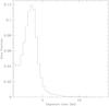 |
Fig. 1 Distribution of the exposure times in the XMM-ATLAS mosaic (bin size: 1 ks). The times are the average between MOS1, MOS2, and PN, for the 0.5−8 keV band; the vertical axis shows the fraction of pixels with a given exposure. |
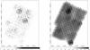 |
Fig. 2 Left: image of the entire mosaic of the XMM-ATLAS observations in the 0.5−8 keV band. The greyscale wedge shows the photon counts (truncated; the actual maximum is 117 counts). A Gaussian smoothing with 20″ radius was applied to enhance the sources. Some areas with longer exposure times and/or higher background are visible. Right: exposure map in the 0.5−8 keV band. The greyscale wedge (maximum value: 33.9 ks) shows the sum of the MOS1, MOS2 and PN exposure times in s, corrected for vignetting and bad pixels. |
To check if astrometric corrections were needed, we performed an initial source detection run with the SAS ewavelet program (with a 5σ threshold) on the PN data of each of the three obsids, and cross-correlated the resulting lists with the sample of QSO from the Sloan Digital Sky Survey (SDSS DR7; Schneider et al. 2010). The search radius was 15″, and most matches were found within 5″. We found that obsid 0725290101 (for which 26 matches were found) needed no correction; obsid 0725300101 (35 matches) had a shift of 0.58″, and obsid 0725310101 (39 matches) of 1.14″. Event and attitude files were corrected (see Table 1) before proceeding further.
Images for the MOS1, MOS2, and PN cameras were accumulated for each obsid and for each of the 0.5−2, 2−8, and 0.5−8 keV bands with a pixel size of 4″ and summed together. Some energy intervals corresponding to known instrumental spectral lines (Kuntz & Snowden 2008, see also R13) were excluded: 1.39−1.55 keV (Al); 1.69−1.80 keV (Si, MOS only); 7.35−7.60 and 7.84−8.28 keV (Cu complex2, PN only). We obtained images of the entire mosaic by summing the images and exposure maps from the three obsids; those relative to the 0.5−8 keV band are shown in Fig. 2.
3. Source detection
Sources were detected with a two-stage process. With our first pass at low significance, we got a list of candidate detections; and on the second pass we raised the significance threshold and derived accurate source parameters. Between the two passes, and because the second pass needs an input catalogue, we identified the sources detected in more than one band. We based the detection method on that used by Cappelluti et al. (2009) and R13 (see also Puccetti et al. 2009), which is a variant on the standard XMM-Newton detection procedure, adapted to the much larger area of XMM-ATLAS.
3.1. First detection pass
In the first pass, the SAS wavelet detection program ewavelet was run separately on each of the 0.5−2, 2−8, and 0.5−8 keV images of the entire mosaic, with a significance threshold of 4σ and the default wavelet scales (minimum 2 pixels, maximum 8 pixels, with a pixel size of 4″).
3.2. Matching sources detected in more than one band
Sources detected in more than one band were identified with the likelihood ratio (LR) technique. Given a distance r between two candidate counterparts, normalised by the uncertainty on the position, LR(r) is defined as the ratio between the probability of having a real counterpart at r over the probability of having a spurious counterpart at r (Pineau et al. 2011)3. Similarly, the association reliability is defined as the probability P(Htrue | r) of the association being true (Htrue) conditioned on r (the relationship between LR and reliability is explicated in Pineau et al. 2011, Eq. (11) and Appendix C).
While the LR is usually applied to search for counterparts in independent bands (e.g. optical counterparts of X-ray sources), here the bands are not independent (we compare the 0.5−8 keV list to the 2−8 keV list; and the 0.5−8 keV list to the 0.5−2 keV list). In this setting, and taking the latter case as an example, we are testing whether the position of the source in both bands is close enough (within errors) to declare that they are the same source, against the possibility that the source of the additional 2−8 keV photons is significantly different from that of the 0.5−2 keV photons. In a shallow survey such as XMM-ATLAS, the main advantage of using the LR method over a nearest-neighbour match is that LR gives a likelihood for the match, which may help in follow-up studies, e.g. when searching for optical counterparts.
We selected the match candidates on the basis of their positional errors; we calibrated the probability of association (items 24 and 25 in the list in Appendix A) estimating a spurious LR histogram. We assigned source IDs at this stage; matched sources were assigned a single ID and are considered as a single source from here onwards.
3.3. Second detection pass, general settings
In the second pass, we used the SAS EMLDetect programme to validate the detection, refine the coordinates and obtain maximum-likelihood estimates of the source counts, count rates and fluxes.
The programme EMLDetect is at its core a PSF fitting code. Originally developed for ROSAT (Cruddace et al. 1988; Hasinger et al. 1993), its current version4 has been improved and optimised for XMM-Newton. In particular, we mention the ability to operate on several individual, overlapping pointings at the same time, and properly account for variations in PSF shape and in vignetting. Since the telescope is moved between pointings, a source may be present in more than one pointing, but may fall on different detector coordinates. Rather than working on a single image containing the entire mosaic (like ewavelet), EMLDetect runs on images of individual pointings (see Sect. 3.4).
Although EMLDetect can run on different energy bands at the same time, we did not use this feature because of the large number of pointings and of EMLDetect limitations (see below), but rather we ran it three times, one per each band. The bands are the same as for ewavelet. In all runs, we used the same input list of sources, made of all matched sources and all unmatched sources, regardless of the bands in which they were detected in the first pass.
The EMLDetect minimum likelihood was set at L = 4.6, as in R13, which corresponds to a false-detection probability of 1.01 × 10⁻². Together with the 4σ threshold for ewavelet, for the final catalogue this yields a joint significance between 4σ and 5σ, but which cannot be further constrained without simulations (see discussion in R13, where a joint significance of 4.8σ was estimated; however this number should not be immediately applied to XMM-ATLAS because of the different statistical properties of the background, due to the different depth of this survey vs. the XMM-CDFS).
We derived the count rate to flux conversion factors assuming a power-law spectrum with photon index Γ = 1.7 and Galactic absorption of NH = 2.3 × 1020 cm-2, and by weighting the responses of the MOS1, MOS2, and PN cameras; they are 5.83 × 10⁻¹², 3.25 × 10⁻¹², and 1.17 × 10⁻¹¹ erg cm-2 for the 0.5−8, 0.5−2, and 2−8 keV bands, respectively.
The 8 keV upper threshold was chosen to improve the signal/noise ratio of detections. While quantities such as counts, rates, and fluxes are quoted in the catalogue for the 0.5−8 and 2−8 keV bands, fluxes in the 0.5−10 and 2−10 keV bands can immediately be obtained assuming the same Γ = 1.7 model spectrum, which yields the following conversion factors for fluxes F: F(0.5−10) /F(0.5−8) = 1.13 and F(2−10) /F(2−8) = 1.20.
We left all EMLDetect parameters, except for those mentioned above (coordinate fitting5, likelihood threshold, energy bands, and conversion factors) at their default values. The inputs to EMLDetect are images, exposure maps (see Sect. 3.4), background maps (see Sect. 3.5), and the list of candidate sources from Sect. 3.2.
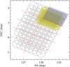 |
Fig. 3 Detection grid for EMLDetect. The grey circles have a radius of 15′ and show the FOV of the individual pointings. The dashed red lines show the grid. The cyan rectangle highlights one of the detection cells. The filled yellow circles are the pointings that intersect the cell and are used for the detection. Only the sources whose coordinates fall into the cell (the rectangle) are kept. This process is repeated for all cells and the final catalogue is the union of the sources from all cells. |
3.4. Splitting a mosaic in individual pointings
To use EMLDetect, we had to split each mosaic-mode obsid event file into the individual pointings; for this purpose we used the SAS tool emosaic_prep. This tool did not set the RA_PNT and Dec_PNT keywords in the individual pointings, which were needed for further processing; however, we obtained the coordinates by inspecting the attitude files.
Images and exposure maps were extracted from each pointing’s event file in the same bands used for ewavelet. We used the SAS task eexpmap to compute the exposure maps; they are in units of s, and include corrections for vignetting and bad pixels. We also computed non-vignetted exposure maps, to be used when producing background maps (Sect. 3.5).
Since the PSF shapes and vignetting are very similar among the three XMM-Newton EPIC cameras, for each pointing we summed together the images from MOS1, MOS2, and PN; then we did the same for the exposure and background maps (see below).
3.5. Background maps
We obtained background maps for the individual pointings with the same method used by the XMM-COSMOS team (Cappelluti et al. 2009). All input sources were excised from the pointing images, producing so-called “cheese images”, in a number of one per pointing per energy band. A model made of a flat (i.e. non-vignetted, but including chip gaps and dead pixels) and a vignetted component (representing the particle and cosmic backgrounds, respectively) was fit to the cheese images to obtain the background maps.
3.6. Running EMLDetect on a wide mosaic
The programme EMLDetect can detect sources on a limited number of overlapping pointings; however, the number of individual pointings in XMM-ATLAS is too large to be analysed together. Therefore, we divided the ATLAS field in a grid. For each cell in the grid (for example, the rectangle in Fig. 3), we identified the pointings whose FOV intersected the cell (filled circles in Fig. 3), and ran EMLDetect on them together. In this way, the number of pointings was within the limit allowed by EMLDetect. From the resulting detection list, we only kept the sources whose coordinates fell into the cell. We checked that no source appears twice, or was lost, by searching for source pairs within 3″ from the cracks. We repeated this procedure for each of the 0.5−8, 0.5−2, and 2−8 keV bands. The final catalogue is the union of the detections from all cells. This approach is similar to that adopted by LaMassa et al. (2013).
The programme which runs EMLDetect in the cells, griddetect, is available (see Appendix B).
3.7. Inspection of close groups
Very close groups of sources with separation much shorter than the PSF width may arise in particular conditions because EMLDetect is fitting the source positions and the detection runs are done separately for the three energy bands. For example, let A and B be two sources from the input catalogue that are present in the same EMLDetect detection cell6. If there are not enough counts for a significant detection by EMLDetect at the input location of A, the programme may try and fit the coordinates until incorrectly assigning them to B’s position; this will then prevent B from getting a detection at the same position and in the same band. This might happen in one energy band but not in another, depending on the details of the two sources (e.g. input coordinates, location of the photons, hardness ratio). Therefore, the same EMLDetect coordinates would be shared by sources A and B, while their ewavelet coordinates would still be different.
To screen and correct for this effect, we have looked for close groups of sources whose EMLDetect coordinates were closer than their 5σ error. We identified 27 groups containing 47 sources in total, and visually inspected all of them. For 22 groups, we shuffled the source ids so that the EMLDetect positions would match the ewavelet positions. Five groups looked like genuine different sources in crowded areas.
3.8. Systematic error on astrometry
To find whether there is any residual systematic error in the XMM-ATLAS astrometry, we cross-correlated the final catalogue with the SDSS QSOs (DR7; Schneider et al. 2010). We found a bulk shift of 0.83″ in RA and − 0.29″ in Dec (XMM-ATLAS coordinate minus SDSS coordinate; root mean square deviation = 2.1″). We subtracted the above values from the XMM-ATLAS coordinates (“RA” and “Dec” columns only, see next Sect.), which should therefore not present any further shift.
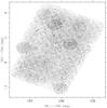 |
Fig. 4 Positions of detected sources, superimposed on the 0.5−8 keV image. |
4. X-ray catalogue
The XMM-ATLAS catalogue includes 1700, 1582, and 814 sources detected by EMLDetect in the 0.5−8, 0.5−2, and 2−8 keV bands, respectively. The number of unique sources is 1816. The flux limits, defined as the flux of the faintest detected sources, are 2 × 10-15, 6 × 10-15, and 9 × 10-15 erg s-1 cm-2 in the 0.5−2, 0.5−8, and 2−8 keV bands, respectively. The positions of the detected sources are shown in Fig. 4, superimposed on a 0.5−8 keV image of the mosaic.
In addition, we list a number of 175, 103, and 47 sources detected in the above bands by ewavelet, but not confirmed by EMLDetect; in the following, we refer to them as supplementary sources. The number of unique supplementary sources is 234.
All coordinates are in the J2000 reference system. The RA and Dec columns are registered to the reference frame of the SDSS-DR7 QSOs (Schneider et al. 2010). All other coordinate columns are not registered and may present a shift; see Sect. 3.8.
The catalogues are available in electronic form from the Centre de Donneés Astronomiques de Strasbourg (CDS), and from the XMM-ATLAS website7, where we will publish updates should they become available.
The description of the catalogue columns is in Appendix A. Hereafter we just clarify the definition of two columns.
The error on position (Col. 8, RADec_ERR) was obtained by dividing the EMLDetect RADec_ERR by  . The RADec_ERR from EMLDetect is computed as
  . However, when two normalised one-dimensional Gaussians of sigma s are combined, the corresponding normalised bi-dimensional Gaussian also has sigma s, not
  , which is what one would get with the expression above. Therefore, we divided the EMLDetect value by .
The error on the hardness ratio (Col. 57, HR_ERR) is defined as  (1)where H and S are the hard (SCTS28) and soft net counts (SCTS052), respectively, and σH (SCTS_ERR28) and σS (SCTS_ERR052) are their errors.
5. Spectra
To investigate the effects of the assumption of a single model spectrum (powerlaw with Γ = 1.7, see Sect. 3), we extracted spectra for 555 sources with more than 40 counts in the 0.5−8 keV band8.
The extraction regions are circles whose radii were chosen by maximizing the signal/noise ratio for each source. The background regions are annuli of inner and outer radii equal to 1.5 and 2 times the circle radius, respectively. In the case of close sources, the overlapping area was excised from the source and background regions. The programme, which defines the regions, autoregions, is available (see Appendix B).
Spectra were extracted using the cdfs-extract tool (see Appendix B), which takes care of identifying the available combinations of event files and source regions. The programme cdfs-extract is a wrapper around the SAS tools evselect, rmfgen, and arfgen to extract spectra and compute the response and ancillary matrices. The MOS and PN spectra were then summed and the response matrices averaged using the FTOOLs mathpha, addrmf, and addarf.
The spectra were automatically analysed with the same method and software (automatic XSPEC fits of unbinned spectra using C-statistic) used for the 3XMM-DR4 sources (Corral et al. 2014). A simple power-law model was fit to the data and used to derive the fluxes in the 0.5−10 and 2−10 keV bands. The fit was successful for 446 sources9. The mean Γ is 1.7 ± 0.6, consistently with the model assumed in Sect. 4. The histogram of best-fit slopes is shown in Fig. 5. We note the presence of a number of flat- and inverted-spectra objects; e.g. there are 56 sources (13 per cent of 446) with Γ ≤ 1.0.
The comparison between the 0.5−10 keV fluxes from the spectral fits and from the catalogue (the latter fluxes converted from 0.5−8 to 0.5−10 keV) is shown in Fig. 6. The distribution of the points around the 1-to-1 line is somewhat asymmetrical for EMLDetect fluxes ≲7 × 10-14 erg s-1 cm-2, with a larger dispersion above the line than below. This is likely due to the combination of the distribution of spectral slopes with the XMM-Newton effective area.
A linear fit to the logarithms of fluxes shown in Fig. 6, obtained by imposing a slope of 1, yielded a normalisation  (2)corresponding to the fluxes from spectral fits being on average (9 ± 4) per cent brighter than those from the catalogue. A dispersion s = 0.31 may be given as the estimate of the standard deviation
  (3)where ν = 1 is the number of free parameters and N is the number of data points, Fspec is the flux from the spectral fit, and Fcat that from the catalogue.
6. The log N−log S
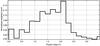 |
Fig. 5 Weighted normalised histogram of best-fit power-law slopes for the XMM-ATLAS sources. The inverse of the fit C-statistics were used as weights. |
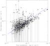 |
Fig. 6 Comparison of fluxes from EMLDetect with fluxes from spectral fits. The blue line shows the 1-to-1 relationship. The fluxes are for the 0.5−10 keV band. |
 |
Fig. 7 Coverage in the 2−10 keV band. |
The sky coverage (sky area as function of flux) for the XMM-ATLAS survey in the 2–8 keV band was derived with the SAS esensmap programme, which creates a sensitivity map by computing count rate upper limits for each pixel. We used the exposure and background maps described in Sect. 3 as input. The resulting coverage was then converted to the 2–10 keV band (Fig. 7).
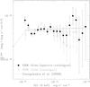 |
Fig. 8 XMM-ATLAS log N–log S in the 2–10 keV band. Filled circles: fluxes from the spectral fits are used whenever possible; catalogue fluxes are used otherwise. Open circles: only fluxes from the catalogue are used; a small horizontal shift has been introduced in the plot to better distinguish the error bars. The solid line shows the best fit to the filled data points. The dashed line is the best-fit model from Georgakakis et al. (2008). The error bars show the 1σ uncertainty. |
We compute the differential counts by binning the sources according to their fluxes  (4)where S is the central flux of the bin; ΔS is the bin width; and for each source i, Ai is the coverage at the source’s flux. The sum is performed on all sources with flux Si ∈ [S − ΔS/ 2,S + ΔS/ 2]. The error on the counts in any bin can be computed by assuming Gaussianity or, for bins with less than 50 sources, with the Gehrels (1986) approximation.
In Fig. 8 we show the 2–10 keV differential log N–log S of the ATLAS sources detected in the 2–8 keV band. Two estimates are shown, from two different sets of fluxes:
-
1.
Spectral log N–log S: fluxes from the spectral fits (Sect. 5) for 387 sources with hard detection, spectrum, and best-fit flux larger than 10-14 erg s-1 cm-2 (the threshold chosen for the faintest bin); plus fluxes from the catalogue (converted to the 2−10 keV band) for the remaining sources (i.e. those without spectra or without a successful fit); and
-
2.
Catalogue log N–log S: fluxes from the catalogue for all the 814 hard sources (also converted to the 2−10 keV band).
The spectral log N–log S extends to brighter fluxes than the catalogue log N–log S, by a factor ≲2, which is consistent with the use for a few sources of a Γ flatter than 1.7.
For comparison, we also plot in Fig. 8 the best-fit model from Georgakakis et al. (2008), which was derived from a joint analysis of several surveys, some of which are much deeper than XMM-ATLAS. The model has a broken power-law shape, with a break flux at 1.2 × 10⁻¹⁴ erg s-1 cm-2, very close the XMM-ATLAS flux limit (at 1.3 × 10⁻¹⁴ erg s-1 cm-2 the coverage is 5.3 per cent of the nominal area, and becomes ill-defined at fainter fluxes). The XMM-ATLAS log N–log S does consistently not show this break.
A linear fit (weighted least squares) to the spectral log N–log S yielded log N = ( − 2.47 ± 0.05)log S − 18.0 ± 0.7 (errors at 1σ), consistent within errors with Georgakakis et al. (2008) and with a Euclidean distribution. A fit to the catalogue log N–log S yielded Log N = ( − 2.37 ± 0.08)Log S − 20.09 ± 1.03, which is only consistent with Euclidean counts at a 2σ level.
7. Conclusions
We have presented the observations, data reduction, catalogue, and number counts of the XMM-ATLAS survey, which covers 7.1 deg2 with flux limits (defined as the flux of the faintest detected sources) of 2 × 10-15, 6 × 10-15, and 9 × 10-15 erg s-1 cm-2 in the 0.5–2, 0.5–8, and 2–8 keV bands, respectively.
We derived the catalogues with a two-step procedure. First, the ewavelet SAS task was used to identify candidate sources with a significance equivalent to 4σ, and to find their coordinates. Next, we used the SAS EMLDetect tool to further check the significance of the sources, and obtain counts, count rates, and fluxes. The final catalogues contain 1700, 1582, and 814 sources in the 0.5–2, 0.5–8, and 2–8 keV bands, respectively, with a total of 1816 unique sources. A list of supplementary sources, detected by ewavelet but not confirmed by EMLDetect, is also provided.
To investigate the effect of assuming a common spectral model for all sources to convert count rates to fluxes, we extracted spectra for each source with at least 40 counts and fitted them with a power-law model. We found that on average, the fluxes from the spectral fits are (9 ± 4) per cent brighter than those from assuming a common power-law photon index of Γ = 1.7. Also, the average best-fit spectral slope is Γ = 1.7 ± 0.6.
We derived the 2–10 keV differential log N–log S for the XMM-ATLAS sources, which spans the 10-14 − 10-12 erg s-1 cm-2 flux interval. Using the fluxes from the spectral fits (for sources with spectra; and fluxes from the catalogue for all other sources) produces a log N–log S, which is less noisy and more consistent with Euclidean counts than using fluxes from the catalogue. A weighted linear fit yielded Log N = ( − 2.47 ± 0.05)Log S − 18.0 ± 0.7 (errors at 1σ); this is consistent, within errors, with previous studies, e.g. Georgakakis et al. (2008).
Finally, we release the software tools that have been developed or enhanced to accomplish the analysis in this paper: griddetect, a programme to run EMLDetect over a very wide mosaic; autoregions, to define extraction regions for spectra and aperture photometry; and cdfs-extract, to extract spectra for multiple sources from multiple observations.
Pineau et al. (2011) also developed an Aladin plugin, which we used for this paper, available at saada.u-strasbg.fr/docs/fxp/plugin/
This column was obtained by dividing the EMLDetect RADec_ERR by ; see Sect. 4.
Acknowledgments
We thank an anonymous referee whose comments have contributed to improve the presentation of this paper. We thank N. Cappelluti for valuable discussions about EMLDetect. P.R. acknowledges a grant from the Greek General Secretariat of Research and Technology in the framework of the programme Support of Postdoctoral Researchers. A.D.M. acknowledges financial support from the UK Science and Technology Facilities Council (ST/I001573/I). F.J.C. acknowledges financial support by the Spanish Ministry of Economy and Competitiveness through grant AYA2012-31447. The use of Virtual Observatory tools is acknowledged (TOPCAT, Taylor 2005, and the Aladin sky atlas, Bonnarel et al. 2000).
References
- Alexander, D. M., & Hickox, R. C. 2012, New A Rev., 56, 93 [NASA ADS] [CrossRef] [Google Scholar]
- Alexander, D. M., Brandt, W. N., Smail, I., et al. 2008, AJ, 135, 1968 [NASA ADS] [CrossRef] [Google Scholar]
- Alonso-Herrero, A., Pereira-Santaella, M., Rieke, G. H., & Rigopoulou, D. 2012, ApJ, 744, 2 [NASA ADS] [CrossRef] [Google Scholar]
- Baldry, I. K., Robotham, A. S. G., Hill, D. T., et al. 2010, MNRAS, 404, 86 [NASA ADS] [Google Scholar]
- Bonnarel, F., Fernique, P., Bienaymé, O., et al. 2000, A&AS, 143, 33 [NASA ADS] [CrossRef] [EDP Sciences] [Google Scholar]
- Brusa, M., Fiore, F., Santini, P., et al. 2009, A&A, 507, 1277 [NASA ADS] [CrossRef] [EDP Sciences] [Google Scholar]
- Cappelluti, N., Brusa, M., Hasinger, G., et al. 2009, A&A, 497, 635 [NASA ADS] [CrossRef] [EDP Sciences] [Google Scholar]
- Cardamone, C. N., Urry, C. M., Schawinski, K., et al. 2010, ApJ, 721, L38 [NASA ADS] [CrossRef] [Google Scholar]
- Chiappetti, L., Clerc, N., Pacaud, F., et al. 2013, MNRAS, 429, 1652 [NASA ADS] [CrossRef] [Google Scholar]
- Civano, F. M. 2013, in AAS/High Energy Astrophysics Division, 13, #116.18 [Google Scholar]
- Corral, A., Georgantopoulos, I., Watson, M. G., et al. 2014, A&A, 569, A71 [NASA ADS] [CrossRef] [EDP Sciences] [Google Scholar]
- Cruddace, R. G., Hasinger, G. R., & Schmitt, J. H. 1988, in European Southern Observatory Conference and Workshop Proc., 28, eds. F. Murtagh, A. Heck, & P. Benvenuti, 177 [Google Scholar]
- Di Matteo, T., Springel, V., & Hernquist, L. 2005, Nature, 433, 604 [NASA ADS] [CrossRef] [PubMed] [Google Scholar]
- Driver, S. P., Norberg, P., Baldry, I. K., et al. 2009, Astron. Geophys., 50, 12 [Google Scholar]
- Eales, S., Dunne, L., Clements, D., et al. 2010, PASP, 122, 499 [NASA ADS] [CrossRef] [Google Scholar]
- Elvis, M., Civano, F., Vignali, C., et al. 2009, ApJS, 184, 158 [NASA ADS] [CrossRef] [Google Scholar]
- Fabian, A. C. 2012, ARA&A, 50, 455 [NASA ADS] [CrossRef] [Google Scholar]
- Ferrarese, L., & Merritt, D. 2000, ApJ, 539, L9 [NASA ADS] [CrossRef] [Google Scholar]
- Gebhardt, K., Bender, R., Bower, G., et al. 2000, ApJ, 539, L13 [NASA ADS] [CrossRef] [Google Scholar]
- Gehrels, N. 1986, ApJ, 303, 336 [NASA ADS] [CrossRef] [Google Scholar]
- Georgakakis, A., Nandra, K., Laird, E. S., et al. 2006, MNRAS, 371, 221 [NASA ADS] [CrossRef] [Google Scholar]
- Georgakakis, A., Nandra, K., Laird, E. S., Aird, J., & Trichas, M. 2008, MNRAS, 388, 1205 [NASA ADS] [CrossRef] [Google Scholar]
- Glazebrook, K., & Economou, F. 1997, The Perl Journal, 5, 5 [Google Scholar]
- Hasinger, G., Burg, R., Giacconi, R., et al. 1993, A&A, 275, 1 [NASA ADS] [Google Scholar]
- Hopkins, P. F., Somerville, R. S., Hernquist, L., et al. 2006, ApJ, 652, 864 [NASA ADS] [CrossRef] [Google Scholar]
- Hopkins, P. F., Hernquist, L., Cox, T. J., & Kereš, D. 2008, ApJS, 175, 356 [NASA ADS] [CrossRef] [Google Scholar]
- Kauffmann, G., & Heckman, T. M. 2009, MNRAS, 397, 135 [NASA ADS] [CrossRef] [Google Scholar]
- Kim, D.-C., Veilleux, S., & Sanders, D. B. 1998, ApJ, 508, 627 [NASA ADS] [CrossRef] [Google Scholar]
- Kuntz, K. D., & Snowden, S. L. 2008, A&A, 478, 575 [NASA ADS] [CrossRef] [EDP Sciences] [Google Scholar]
- LaMassa, S. M., Urry, C. M., Cappelluti, N., et al. 2013, MNRAS, 436, 3581 [NASA ADS] [CrossRef] [Google Scholar]
- Lamastra, A., Menci, N., Fiore, F., et al. 2013, A&A, 559, A56 [NASA ADS] [CrossRef] [EDP Sciences] [Google Scholar]
- Lanzuisi, G., Ranalli, P., Georgantopoulos, I., et al. 2015, A&A, 573, A137 [NASA ADS] [CrossRef] [EDP Sciences] [Google Scholar]
- Lehmer, B. D., Alexander, D. M., Bauer, F. E., et al. 2010, ApJ, 724, 559 [NASA ADS] [CrossRef] [Google Scholar]
- Lutz, D., Mainieri, V., Rafferty, D., et al. 2010, ApJ, 712, 1287 [NASA ADS] [CrossRef] [Google Scholar]
- Menci, N., Rosati, P., Gobat, R., et al. 2008, ApJ, 685, 863 [NASA ADS] [CrossRef] [Google Scholar]
- Mullaney, J. R., Daddi, E., Béthermin, M., et al. 2012a, ApJ, 753, L30 [NASA ADS] [CrossRef] [Google Scholar]
- Mullaney, J. R., Pannella, M., Daddi, E., et al. 2012b, MNRAS, 419, 95 [NASA ADS] [CrossRef] [Google Scholar]
- Nardini, E., & Risaliti, G. 2011, MNRAS, 415, 619 [NASA ADS] [CrossRef] [Google Scholar]
- Nardini, E., Risaliti, G., Watabe, Y., Salvati, M., & Sani, E. 2010, MNRAS, 405, 2505 [NASA ADS] [Google Scholar]
- Oliver, S. J., Bock, J., Altieri, B., et al. 2012, MNRAS, 424, 1614 [NASA ADS] [CrossRef] [EDP Sciences] [Google Scholar]
- Pierce, C. M., Lotz, J. M., Primack, J. R., et al. 2010, MNRAS, 405, 718 [NASA ADS] [Google Scholar]
- Pierre, M., Valtchanov, I., Altieri, B., et al. 2004, J. Cosmol. Astropart. Phys., 9, 11 [Google Scholar]
- Pineau, F.-X., Motch, C., Carrera, F., et al. 2011, A&A, 527, A126 [NASA ADS] [CrossRef] [EDP Sciences] [Google Scholar]
- Puccetti, S., Vignali, C., Cappelluti, N., et al. 2009, ApJS, 185, 586 [NASA ADS] [CrossRef] [Google Scholar]
- Ranalli, P., Comastri, A., Vignali, C., et al. 2013, A&A, 555, A42 [NASA ADS] [CrossRef] [EDP Sciences] [Google Scholar]
- Rigby, E. E., Maddox, S. J., Dunne, L., et al. 2011, MNRAS, 415, 2336 [NASA ADS] [CrossRef] [Google Scholar]
- Rovilos, E., & Georgantopoulos, I. 2007, A&A, 475, 115 [NASA ADS] [CrossRef] [EDP Sciences] [Google Scholar]
- Rovilos, E., Comastri, A., Gilli, R., et al. 2012, A&A, 546, A58 [Google Scholar]
- Ruiz, A., Risaliti, G., Nardini, E., Panessa, F., & Carrera, F. J. 2013, A&A, 549, A125 [NASA ADS] [CrossRef] [EDP Sciences] [Google Scholar]
- Schneider, D. P., Richards, G. T., Hall, P. B., et al. 2010, AJ, 139, 2360 [NASA ADS] [CrossRef] [Google Scholar]
- Silk, J., & Rees, M. J. 1998, A&A, 331, L1 [NASA ADS] [Google Scholar]
- Taylor, M. B. 2005, in Astronomical Data Analysis Software and Systems XIV, eds. P. Shopbell, M. Britton, & R. Ebert, ASP Conf. Ser., 347, 29 [Google Scholar]
- Tran, Q. D., Lutz, D., Genzel, R., et al. 2001, ApJ, 552, 527 [NASA ADS] [CrossRef] [Google Scholar]
- Trichas, M., Georgakakis, A., Rowan-Robinson, M., et al. 2009, MNRAS, 399, 663 [NASA ADS] [CrossRef] [Google Scholar]
- Veilleux, S., Kim, D.-C., & Sanders, D. B. 1999, ApJ, 522, 113 [NASA ADS] [CrossRef] [Google Scholar]
- Viero, M. P., Asboth, V., Roseboom, I. G., et al. 2014, ApJS, 210, 22 [NASA ADS] [CrossRef] [Google Scholar]
- Zubovas, K., & King, A. R. 2012, MNRAS, 426, 2751 [NASA ADS] [CrossRef] [Google Scholar]
Appendix A: Catalogue description
The column description of the catalogue columns is as follows (the symbols (ML) and (W) mark whether the column was derived from running EMLDetect or ewavelet, respectively):
-
1.
IAU_IDENTIFIER − source identifier following International Astronomical Union conventions;
-
2.
ID − unique source number;
-
3–5.
ID058, ID052, ID28;
-
6.
RA − (ML) right ascension (degrees) from the 0.5–8 keV band, if available; else, from the 0.5–2 keV band, if available; else, from the 2–8 keV band. This column has been corrected for astrometry and registered to the SDSS-DR7 QSO framework;
-
7.
Dec − (ML) declination (degrees) as above. This column has been corrected for astrometry and registered to the SDSS-DR7 QSO framework;
-
8.
RADec_ERR − (ML) error on position10 (arcsec; 1σ);
-
9.
WAV_RA − (W) merged right ascension (degrees) from the likelihood ratio;
-
10.
WAV_Dec − (W) merged declination (degrees);
-
11.
WAV_RADec_ERR − (W) merged error on position (arcsec; 1σ);
-
12.
WAV_RA058 − (W) right ascension (degrees) in the 0.5−8 keV band;
-
13.
WAV_Dec058 − (W) declination (degrees) in the 0.5−8 keV band;
-
14.
WAV_RA052 − (W) right ascension (degrees) in the 0.5−2 keV band;
-
15.
WAV_Dec052 − (W) declination (degrees) in the 0.5−2 keV band;
-
16.
WAV_RA28 − (W) right ascension (degrees) in the 2−8 keV band;
-
17.
WAV_Dec28 − (W) declination (degrees) in the 2−8 keV band;
-
18.
RA058 − (ML) right ascension (degrees) in the 0.5−8 keV band;
-
19.
Dec058 − (ML) declination (degrees) in the 0.5−8 keV band;
-
20.
RA052 − (ML) right ascension (degrees) in the 0.5−2 keV band;
-
21.
Dec052 − (ML) declination (degrees) in the 0.5−2 keV band;
-
22.
RA28 − (ML) right ascension (degrees) in the 2−8 keV band;
-
23.
Dec28 − (ML) declination (degrees) in the 2−8 keV band;
-
24.
ASSOC_RELIAB058052 − association reliability between the (WAV_RA058, WAV_Dec058) and (WAV_RA052, WAV_Dec052) coordinates;
-
25.
ASSOC_RELIAB05828 − association reliability between the (WAV_RA058, WAV_Dec058) and (WAV_RA28, WAV_Dec28) coordinates;
-
26–28.
SCTS058, SCTS052, SCTS28 − (ML) sum of the net source counts from MOS1+MOS2+PN in the 0.5−8, 0.5−2 and 2−8 keV bands, respectively;
-
29–31.
SCTS_ERR058, SCTS_ERR052, SCTS_ERR28 − (ML) errors on SCTS058, SCTS052, SCTS28 (1σ);
-
32–34.
RATE058, RATE052, RATE28 − (ML) net count rates in the 0.5–8, 0.5–2, 2–8 keV bands, averaged over the three cameras;
-
35–37.
EXP_MAP058, EXP_MAP052, EXP_MAP28 − exposure times in the 0.5−8, 0.5−2, 2−8 keV bands, summed over the three cameras;
-
38–40.
BG_MAP058, BG_MAP052, BG_MAP28 − (ML) background counts/arcsec2 in the 0.5−8, 0.5−2, 2−8 keV bands, summed over the three cameras;
-
41–43.
FLUX058, FLUX052, FLUX28 − (ML) flux in the 0.5–8, 0.5–2, 2–8 keV bands (erg s-1 cm-2);
-
44–46.
FLUX_ERR058, FLUX_ERR052, FLUX_ERR28 − (ML) error on FLUX058, FLUX052, FLUX28 (1σ);
-
47–49.
DETML058, DETML052, DETML28 − (ML) detection likelihoods in the 0.5–8, 0.5–2, 2–8 keV bands;
-
50–51.
EXT058, EXT052 – (ML) source extent in the 0.5−8 and 0.5−2 keV bands11 (σ of Gaussian model in pixels; 1 pixel = 4″);
-
52−53.
EXT_ERR058, EXT_ERR052 − (ML) error on EXT058, EXT052 (1σ);
-
54−55.
EXT_ML058, EXT_ML052 − (ML) likelihood of extent in the 0.5−8 and 0.5−2 keV bands;
-
56.
HR − hardness ratio, computed from S = SCTS052 and H = SCTS28 as HR = (H − S) / (H + S);
-
57.
HR_ERR − error on HR (1σ; see Sect. 4).
The columns from 58 to 87 contain source properties (counts, count rates, fluxes, exposure times, background, wavelet detection scale, source extent) from ewavelet; while we report these for all sources, they are actually only interesting for supplementary sources.
-
58–60.
WAV_SCTS058, WAV_SCTS052, WAV_SCTS28 − (W) sum of the net source counts from MOS1+MOS2+PN in the 0.5−8, 0.5−2, and 2−8 keV bands, respectively;
-
61–63.
WAV_SCTS_ERR058, WAV_SCTS_ERR052, WAV_SCTS_ERR28 − (W) errors on SCTS058, SCTS052, SCTS28 (1σ);
-
64–66.
WAV_RATE058, WAV_RATE052, WAV_RATE28 − (W) net count rates in the 0.5−8, 0.5−2, 2−8 keV bands, averaged over the three cameras;
-
67–69.
WAV_EXP_MAP058, WAV_EXP_MAP052, WAV_EXP_MAP28 − (W) exposure times in the 0.5−8, 0.5−2, 2−8 keV bands, summed over the three cameras;
-
70–72.
WAV_BG_MAP058, WAV_BG_MAP052, WAV_BG_MAP28 − (W) background counts/arcsec2 in the 0.5−8, 0.5−2, 2−8 keV bands, summed over the three cameras;
-
73–75.
WAV_FLUX058, WAV_FLUX052, WAV_FLUX28 − (W) fluxes in the 0.5−8, 0.5−2, 2−8 keV bands (erg s-1 cm-2);
-
76–78.
WAV_FLUX_ERR058, WAV_FLUX_ERR052, WAV_FLUX_ERR28 − (W) errors on WAV_FLUX058, WAV_FLUX052, WAV_FLUX28 (1σ);
-
79–81.
WAV_WSCALE058, WAV_WSCALE052, WAV_WSCALE28 − (W) wavelet detection scale (pixels; 1 pixel = 4″);
-
82–84.
WAV_EXTENT058, WAV_EXTENT052, WAV_EXTENT28 − (W) source extent (pixels);
-
85–87.
WAV_EXT_ERR058, WAV_EXT_ERR052, WAV_EXT_ERR28 − (W) errors on WAV_EXTENT058, WAV_EXTENT052, WAV_EXTENT28 (1σ; pixels).
Appendix B: Released software
For the software described below, more information and instructions for their use can be found on the author’s website12 and source repository13.
cdfs-extract and autoregions
Given a number of event files and a list of source and background positions, the cdfs-extract programme checks if the source and background are in the field of view of any observation, and it extracts products accordingly. The observations may or may not overlap.
The extracted products are spectra (source and background) and responses (source and, optionally, background RMFs and ARFs), or aperture photometry, or light curves.
The programme takes as input two text files, containing:
-
a list of event files, exposure maps and (optional) images;
-
a list of source and background positions and radii (the camera may be specified optionally, allowing the same source to have different positions or radii for different cameras).
Spectra and responses can be summed if the user wants, producing a single spectral file for each source and each camera.
The list of source and background positions can be either be manually written, or automatically produced by autoregions. If the sources are not too close to each other and the background has no large variations on scales ≲20−30″, then annuli can be used as background regions and their positions and radii can be automatically generated (i.e. the user is dealing with a shallow survey such as XMM-ATLAS, XXL or XMM-COSMOS; conversely, deep surveys such as the XMM-CDFS feature close groups of sources and complex spatial patterns in the background, which make automatic procedures unreliable).
Given a catalogue of sources, stored in a database (e.g. PostgreSQL) and containing source counts and background surface brightnesses (i.e. the EMLDetect output), the autoregions programme computes extraction regions through maximizing the expected signal/noise ratio. Overlapping regions are identified, and where possible, the overlapping areas are excised.
Besides this work, the programmes described above have been, or are being used, in several papers, e.g. the obscured AGN in XMM-COSMOS (Lanzuisi et al. 2015), the XMM-CDFS spectral survey (Comastri et al., in prep.), the XXL brightest AGN spectral survey (Fotopoulou et al., in prep.).
Both cdfs-extract and autoregions are written in (modern-style) Perl using the Perl Data Language (PDL) libraries (Glazebrook & Economou 1997, pdl.perl.org), and are free software released under the terms of the GNU Affero GPL license14.
griddetect and associated libraries
The motivation for griddetect, and how it works, have already been described in Sect. 3.6 (see also Fig. 3).
Here we also mention that the XMM-Newton SAS provides a tool (emosaicproc), whose functionality is partly duplicated by griddetect. The main difference between the tools may be summarised as follows: emosaicproc automatically computes the grid, and requires less data preparation by the user if a single mosaic-mode obsid is to be processed, but only works on a single obsid; griddetect needs the user to define the grid cracks, but it is easier to add pointings from different obsids, and it can also compute background maps.
The programme griddetect works on individual pointings, splitted from mosaic-mode event files; it also computes background maps according to the Cappelluti et al. (2009) method. The input comprises:
-
the grid specification: a rotation angle, and the x and y coordinates(rotated RA and Dec) of the grid lines;
-
the list of pointings with their coordinates.
The output is a series of two catalogues per detection cell: one containing the detected sources, and another containing only the sources within 3″ from the cracks (used to check if there are missing or repeated sources, arising because of numeric effects placing them alternatively on the two sides of the crack).
Together with griddetect, we also release a set of associated libraries that may be of more general purpose: XMMSAS::Extract and XMMSAS::Detect. These are object-oriented Perl packages, which present a high-level interface to some SAS and FTOOLS commands. They can be called by Perl programmes to filter event files and extract images and exposure maps using either pre-defined filters (e.g. the instrumental lines excluded in Sect. 2) or user-defined filters; and to compute background maps, source masks and call EMLDetect.
The programme griddetect and its associated libraries are written in (modern-style) Perl using the Moose object system and the Perl Data Language (PDL) libraries (Glazebrook & Economou 1997, pdl.perl.org), and are free software released under the terms of the GNU Affero GPL license.
All Tables
All Figures
|
Fig. 1 Distribution of the exposure times in the XMM-ATLAS mosaic (bin size: 1 ks). The times are the average between MOS1, MOS2, and PN, for the 0.5−8 keV band; the vertical axis shows the fraction of pixels with a given exposure. |
| In the text | |
|
Fig. 2 Left: image of the entire mosaic of the XMM-ATLAS observations in the 0.5−8 keV band. The greyscale wedge shows the photon counts (truncated; the actual maximum is 117 counts). A Gaussian smoothing with 20″ radius was applied to enhance the sources. Some areas with longer exposure times and/or higher background are visible. Right: exposure map in the 0.5−8 keV band. The greyscale wedge (maximum value: 33.9 ks) shows the sum of the MOS1, MOS2 and PN exposure times in s, corrected for vignetting and bad pixels. |
| In the text | |
|
Fig. 3 Detection grid for EMLDetect. The grey circles have a radius of 15′ and show the FOV of the individual pointings. The dashed red lines show the grid. The cyan rectangle highlights one of the detection cells. The filled yellow circles are the pointings that intersect the cell and are used for the detection. Only the sources whose coordinates fall into the cell (the rectangle) are kept. This process is repeated for all cells and the final catalogue is the union of the sources from all cells. |
| In the text | |
|
Fig. 4 Positions of detected sources, superimposed on the 0.5−8 keV image. |
| In the text | |
|
Fig. 5 Weighted normalised histogram of best-fit power-law slopes for the XMM-ATLAS sources. The inverse of the fit C-statistics were used as weights. |
| In the text | |
|
Fig. 6 Comparison of fluxes from EMLDetect with fluxes from spectral fits. The blue line shows the 1-to-1 relationship. The fluxes are for the 0.5−10 keV band. |
| In the text | |
|
Fig. 7 Coverage in the 2−10 keV band. |
| In the text | |
|
Fig. 8 XMM-ATLAS log N–log S in the 2–10 keV band. Filled circles: fluxes from the spectral fits are used whenever possible; catalogue fluxes are used otherwise. Open circles: only fluxes from the catalogue are used; a small horizontal shift has been introduced in the plot to better distinguish the error bars. The solid line shows the best fit to the filled data points. The dashed line is the best-fit model from Georgakakis et al. (2008). The error bars show the 1σ uncertainty. |
| In the text | |
Current usage metrics show cumulative count of Article Views (full-text article views including HTML views, PDF and ePub downloads, according to the available data) and Abstracts Views on Vision4Press platform.
Data correspond to usage on the plateform after 2015. The current usage metrics is available 48-96 hours after online publication and is updated daily on week days.
Initial download of the metrics may take a while.