| Issue |
A&A
Volume 576, April 2015
|
|
|---|---|---|
| Article Number | A20 | |
| Number of page(s) | 18 | |
| Section | Galactic structure, stellar clusters and populations | |
| DOI | https://doi.org/10.1051/0004-6361/201425239 | |
| Published online | 16 March 2015 | |
Polarized light from Sagittarius A* in the near-infrared Ks-band⋆,⋆⋆
1 I. Physikalisches Institut, Universität zu Köln, Zülpicher Str. 77, 50937 Köln, Germany
e-mail: This email address is being protected from spambots. You need JavaScript enabled to view it.
2 Max-Planck-Institut für Radioastronomie, Auf dem Hügel 69, 53121 Bonn, Germany
3 Department of Physics and Astronomy, University of California, Los Angeles, CA 90095, USA
4 Astronomical Institute, Academy of Sciences, Boční II 1401, 14131 Prague, Czech Republic
5 Institut de Recherche en Astrophysique et Planétologie (IRAP) Université de Toulouse, CNRS Observatoire Midi-Pyrénées (OMP), 14 avenue Édouard Belin, 31400 Toulouse, France
Received: 30 October 2014
Accepted: 7 January 2015
Abstract
We present a statistical analysis of polarized near-infrared light from Sgr A*, the radio source associated with the supermassive black hole at the center of the Milky Way. The observations were carried out using the adaptive optics instrument NACO at the VLT UT4 in the infrared Ks-band from 2004 to 2012. Several polarized flux excursions were observed during these years. Linear polarization at 2.2 μm, its statistics, and time variation, can be used constrain the physical conditions of the accretion process onto this supermassive black hole. With an exponent of about 4 for the number density histogram of fluxes above 5 mJy, the distribution of polarized flux density is closely linked to the single state power-law distribution of the total Ks-band flux densities reported earlier. We find typical polarization degrees on the order of 20% ± 10% and a preferred polarization angle of 13° ± 15°. Simulations show the uncertainties under a total flux density of ~2 mJy are probably dominated by observational effects. At higher flux densities there are intrinsic variations of polarization degree and angle within well constrained ranges. Since the emission is most likely due to optically thin synchrotron radiation, the preferred polarization angle we find is very likely coupled to the intrinsic orientation of the Sgr A* system, i.e. a disk or jet/wind scenario associated with the supermassive black hole. If they are indeed linked to structural features of the source the data imply a rather stable geometry and accretion process for the Sgr A* system.
Key words: black hole physics / infrared: general / accretion, accretion disks / Galaxy: center / Galaxy: nucleus / galaxies: statistics
Based on NACO observations collected between 2004 and 2012 at the Very Large Telescope (VLT) of the European Organization for Astronomical Research in the Southern Hemisphere (ESO), Chile.
Appendix A is available in electronic form at http://www.aanda.org
© ESO, 2015
1. Introduction
Sagittarius A* (Sgr A*) is a bright and compact radio source associated with a supermassive black hole (MBH ~ 4 × 10⁶M⊙) located at the center of our galaxy (Eckart & Genzel 1996, 1997; Eckart et al. 2002; Schödel et al. 2002; Eisenhauer et al. 2003; Ghez et al. 1998, 2000, 2005, 2008; Gillessen et al. 2009); it is the best example of a low-luminosity galactic nucleus accessible to observations. Sgr A* shows time variability in high spatial resolution observations in the near-infrared (NIR) and X-ray regime compared to a lower degree of variability in the radio to sub-mm domain. The NIR counterpart to Sgr A* shows short bursts of increased radiation that can occur four to six times per day and last about 100 min.
Analyzing the polarization of the electromagnetic radiation can help us to reveal the nature of emission processes detected from Sgr A*. Therefore, this source has been observed since 2004 in the polarimetric imaging mode with NACO using its Wollaston prism (Eckart et al. 2006a, 2008a; Meyer et al. 2006a,b; Zamaninasab et al. 2010; Witzel et al. 2012). Multi-wavelength observations have been conducted by different research groups to study the spectral energy distribution (SED) and the variable emission process of Sgr A* from the radio to the X-ray domain (Baganoff et al. 2001; Porquet et al. 2003; Genzel et al. 2003; Eckart et al. 2004, 2012, 2006a,b,c, 2008a,b; Meyer et al. 2006a,b, 2007; Yusef-Zadeh et al. 2006b,a, 2007, 2008; Dodds-Eden et al. 2009; Sabha et al. 2010). Observations at 1.6 μm and 1.7 μm wavelengths using the Hubble Space Telescope (HST; Yusef-Zadeh et al. 2009) indicate that the activity of Sgr A* is above the noise level more than 40% of the time. The highly polarized NIR flux density excursions usually have X-ray counterparts, which suggests a synchrotron-self-Compton (SSC) or inverse Compton emission as the responsible radiation mechanism (Eckart et al. 2004, 2006a,c, 2012; Yuan et al. 2004; Liu et al. 2006). Several relativistic models that successfully describe the observations presume the variability to be related to the emission from single or multiple spots close to the last stable orbit of the black hole (Meyer et al. 2006a,b, 2007; Zamaninasab et al. 2008).
Based on a model in which matter is orbiting the supermassive black hole Sgr A* with relativistic speed, Zamaninasab et al. (2010) predict and explore a correlation between the modulations of the observed flux density light curves and changes in polarization dergee and position angle. This information should in principle allow us to constrain the spin of the black hole (assuming that the gravitational field is indeed described by the Kerr metric). However, the question of whether timescales comparable to the orbital period near the inner edge of the accretion flow (in particular, near the radius of the innermost stable orbit) play a role in the variability, was (and still remains) impossible to decide on the basis of available data. Although the geometrical effects of strong gravitational fields act on photons independently of their energy, the intrinsic emissivity of accretion disks and the influence of a magnetic field are energy dependent. Therefore, the variability amplitudes of both the polarization degree and the polarization angle are expected to be energy dependent as well. These dependencies suffer from degeneracy. These degeneracies and the interdependencies of the observables require both time-resolved observations (e.g. Zamaninasab et al. 2010) and a statistical analysis as presented here.
Witzel et al. (2012) show that the time variable NIR emission from Sgr A* can be understood as a consequence of a single continuous power-law process with a break timescale between 500 and 700 min. This continuous process shows extreme flux density excursions that typically last for about 100 min. In the following we will refer to these excursions as flares, and that they occur as flaring activity. On the basis of multi-wavelength observations in 2009, Eckart et al. (2012) show that the flaring activity can be modeled as a signal from a synchrotron/synchrotron-self-Compton component.
Several authors have studied the statistical properties of flaring activity of Sgr A* instead of concentrating on investigating the individual flares. Do et al. (2009) do not find quasiperiodic oscillations (QSOs), which can be related to the orbital time of the matter in the inner part of an accretion disk, against the pure red noise while probing 7 total intensity NIR light curves taken with Keck telescope. The authors also conclude that Sgr A* is continuously variable. The red power-law distribution of the variable emission at NIR can be described by fluctuations in the accretion disk (Chan et al. 2009). However, the correlation between flux density modulations and changes in the degree of polarization, the delayed sub-mm emission, and the SED show that the emission is coming from a compact flaring region with a size close to the Schwarzschild radius. This compact region can be a jet with blobs of ejected material (Markoff et al. 2001) or a radiating hot spot(s) falling into the black hole (see e.g. Genzel et al. 2003; Dovčiak et al. 2004, 2008; Eckart et al. 2006b; Gillessen et al. 2006; Meyer et al. 2006a; Hamaus et al. 2009; Zamaninasab et al. 2010). Amongst the first papers that introduce the concept of orbiting hot spots in the context of black hole accretion disks in a constructive way are Doi (1978) and Pineault (1980). In the case of Cyg X-1, bursts of X-ray emission were explained via this concept (Doi 1978). For the supermassive black hole in AO 0235+164 it was used to explain variability in total flux and polarization properties (Pineault 1980).
The statistics of NIR Ks-band total intensity variability of Sgr A* observed from 2004 to 2009 with the VLT, has been investigated by Dodds-Eden et al. (2011). The authors interpret the time variability of Sgr A* as a two state process, a quiescent state for low fluxes (below 5 mJy) which has a log-normal distribution and a flaring state for high fluxes (above 5 mJy) that has a power-law distribution. From their analysis they claim that the physical processes responsible for the low and high flux densities from Sgr A* are different. However, their conclusions for the low flux densities are based on data at or below the detection limit, and therefore is biased by the measurements uncertainties and source crowding. On the other hand, Witzel et al. (2012) show, for their slightly larger data set taken between 2003 and early 2010, that the variability of Sgr A* is well described by a single power-law distribution, and conclude that there is no evidence for a second intrinsic state based on the distribution of flux densities. Meyer et al. (2014) come to a similar result modeling the data by a rigorous two state regime switching time series that additionally included the information on the timing properties of Sgr A*. These results unambiguously show that in the range of reliably measurable fluxes the variability process can be described as a continuous, single state red-noise process with a characteristic timescale of several hours, without any characteristic flux density.
The analysis of the intrinsic polarization degree and polarization angle of the emission from Sgr A* and their changes during the flaring activity is another important aspect of the time variability. In this paper we analyze the most comprehensive sample of NIR polarimetric light curves of Sgr A*. In Sect. 2 we provide details about the observations and data reduction. In Sect. 3, we present the statistical analysis of polarized flux densities, a comparison with total flux densities and their distribution as provided by Witzel et al. (2012). In Sect. 4 we summarize the results and discuss their implications.
2. Observations and data reduction
All observations for this paper have been carried out with the adaptive optics (AO) module NAOS and NIR camera CONICA (together NACO; Lenzen et al. 2003; Rousset et al. 2003) at the UT4 (Yepun) at the Very Large Telescope (VLT) of the European Southern Observatory (ESO) on Paranal, Chile. We collected all Ks-band (2.2 μm) observational data of the central cluster of the Galactic center (GC) in 13 mas pixel scale polarimetry with the camera S13 from mid-2004 to mid-2012 that have flare events. In all the selected observations the infrared wavefront sensor of NAOS was used for locking the AO loop on the NIR supergiant IRS7 with Ks~6.5−7.0 mag, located ~5.5′′ north from Sgr A*. NACO is equipped with a Wollaston prism combined with a half-wave retarder plate that provide simultaneous measurements of two orthogonal directions of the electric field vector and a rapid change between different angles of the electric field vector.
In the following we present a short summary of the reduction steps. For 2004 to 2009 we used the reduced data sets as presented in Witzel et al. (2012). The 27 May 2011 and 17 May 2012 data have not been published before and we applied an observational strategy and data reduction steps similar to Witzel et al. (2012) to these data sets. The AO correction for the 27 May 2011 and 17 May 2012 nights, was most of the time stable and in good seeing condition. We had Sgr A* and a sufficient number of flux secondary density calibrators in the innermost arcsecond. The observing dates, integration times, sampling rate and mean flux densities of the data sets used for our analysis are presented in Table 1.
Observations log.
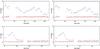 |
Fig. 1 NIR Ks-band (2.2 μm) light curves of Sgr A* observed in polarimetry mode on 27 May 2011 (top) and 17 May 2012 (bottom) produced by combining pairs of orthogonal polarization channels; left: 0°, 90° and right: 45°, 135°. The blue dots show Sgr A* flux density measured in mJy, while the red connected dots show the background flux densities. |
All the exposures were sky subtracted, flat fielded and bad pixel corrected. We used lamp flat fields, instead of sky flat fields to avoid polarimetric effects produced by the sky. Since the exposures were dithered, all the polarization channels (0°, 45°, 90°, 135°) of the individual data set were aligned with using a cross-correlation method with sub-pixel accuracy (Devillard 1999). The point spread functions (PSFs) were extracted from the images with the IDL routine Starfinder (Diolaiti et al. 2000) using isolated stars close to Sgr A*.
We used the Lucy-Richardson algorithm to deconvolve the images. Image restoration was done by convolving the deconvolved images with a Gaussian beam of a full width at half maximum of about 60 mas corresponding to the diffraction limit at 2.2 μm. Using the Lucy-Richardson algorithm (Lucy 1974; Richardson 1972) allows us to separate the flux density contributions of very close sources. Ott et al. (1999) have shown in particular for the GC that deconvolution algorithms like Lucy, Clean and Wiener filtering work very well and reproduce the flux densities down to the detection limit. The effect of weak residuals resulting from a combination of the positivity constraint for the Lucy-Richardson algorithm and a faint background mostly dominated by the superpositon of extended seeing foots, is monitored through the off-appertures to measure the background. The contribution lies well below the detection limit for faint flares (see below).
2.1. Flux density calibration
We measured the flux densities of Sgr A* and other compact sources in the field by aperture photometry using circular apertures of 40 mas radius. The flux density calibration was carried out using the known Ks-band flux densities of 13 S-stars (Schödel et al. 2010). Furthermore, 6 comparison stars and 8 background apertures placed at positions where no individual sources are detected. For more details about the positions of the apertures and the list of calibrators see Fig. 2 of this paper and Table 1 in Witzel et al. (2012). To get the total flux densities we added up the photon counts in each aperture and then added the resultant values of two orthogonal polarimetry channels. These values were corrected for the background contribution. We calculated the flux densities of the calibrators close to Sgr A* and also at the position of Sgr A* and then corrected them for extinction using AKs = 2.46, derived for the inner arcsecond by Schödel et al. (2010). Applying aperture photometry on all frames, results in the light curves obtained for Sgr A* in two orthogonal channels for 27 May 2011 and 17 May 2012 data, as shown in Fig. 1.
The gaps in the measurements are due to AO reconfiguration or sky measurements. For 27 May 2011 data the flux density of Sgr A* varied between about 5 and 10 mJy over the entire observing run. For 17 May 2012 data, over the first 50 min, the flux density of Sgr A* increased to about 7 mJy and then decreased again.
Figure 2 shows a Ks-band deconvolved image of the GC on 17 May 2012. The image is taken with the ordinary beam of the Wollaston prism. The positions of Sgr A*, calibration stars and comparison apertures for background estimates are shown. For comparison see also Fig. 1 from 30 September 2004 by Witzel et al. (2012). Source identification has been done using the nomenclature by Gillessen et al. (2009).
The flux density of Sgr A* was calculated from the flux densities measured in the four different polarization channels and corrected for possible background contributions. The top panel of Fig. 3 shows the measured flux density distributions of different calibration stars close to Sgr A* fitted by Gaussian functions. The scatter of the flux densities around the mean value originates from the observational uncertainties and can be estimated from these fits. The standard deviations σ of the Gaussians fitted to the distributions are presented as a function of the mean flux density in the bottom panel of Fig. 3. The function that best describes the dependency of σ values with the flux densities up to 33 mJy is a second degree polynomial that tends to be flatter at small flux density values.
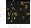 |
Fig. 2 Ks-band deconvolved image of the GC on 17 May 2012 showing the positions of Sgr A*, calibration stars and comparison apertures for background estimates marked by yellow circles. |
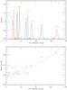 |
Fig. 3 Top: normalized flux density distributions of 10 flux calibrators of Sgr A*. The dashed lines are Gaussian fits to the distributions. Bottom: standard deviation of flux densities of calibration stars versus flux densities of them. The red line is the polynomial fit to the measured σ values of the calibrators shown in the upper panel (red crosses). The two purple x symbols present the measured error values (obtained by Witzel et al. 2012) at the position of the comparison apertures for the background emission close to the position of Sgr A* (see Fig. 2). |
While using a second degree polynomial is a prior unphysical, it allows us to asses the quality of the data and compares it to the previous works (Witzel et al. 2012; Do et al. 2009) who have used a similar approach. The measured flux densities and scatter of the two background apertures (C1 and C2 in Fig. 2) have been added to the plot and included the fit. The uncertainties up to 10 mJy total flux are ~0.25 mJy and are mostly introduced by a combination of a variation in the AO performance, imperfectly subtracted PSF seeing halos of surrounding, brighter stars and differential tilt jitter. Within the uncertainties and for a total flux density value below 10 mJy this relation is in good agreement with that found by Witzel et al. (2012) using a larger sample of total flux density measurements shown in their Fig. 7. However, our data shows 20% to 25% narrower flux density distributions at higher flux values around 30 mJy because polarization data tend to be observationally biased towards higher Strehl values compared to AO imaging in standard observer mode, i.e. without selection of preferred atmospheric conditions. The result shown in Fig. 3 also implies that statements on the source intrinsic total or polarized flux density of Sgr A* can only be made with certainty if the total flux density is significantly larger than the limit of ~0.25 mJy.
2.2. Polarimetry
Using non-normalized analog-to-digital converter (ADC) values from the detector (see details in Witzel et al. 2011) to obtain normalized stokes parameters we can derive the polarization degree and angle,  where f0, f45, f90, and f135 are the four polarimetric channels flux densities with f0, f90 and f45, f135 being pairs of orthogonally polarized channels. The variable F represents the total flux density and Q and U are the normalized Stokes parameters. No information on the circular polarization in normalized Stokes V is available with NACO, hence the circular polarization is assigned to zero (see Witzel et al. 2011 for a detailed discussion). The quantity p is the degree of polarization and φ is the polarization angle which is measured from the north to the east and samples a range between 0° and 180°. We compute the polarized flux density as the product of the degree of polarization and the total flux density. Uncertainties for F, Q, U and the obtained p and φ were determined from the flux density uncertainties. Since NACO is a Nasmyth focus camera-system, instrumental effects can influence our results and a careful calibration is needed. Witzel et al. (2011) used the Stokes/Mueller formalism to describe the instrumental polarization. Their analytical model applies Mueller matrices to the derived normalized Stokes parameters to get the intrinsic normalized Stokes parameters. We used their model to diminish the systematical uncertainties of polarization angles and degrees caused by instrumental polarization to about ~1% and ~5°, respectively. Foreground polarization has been obtained for the stars in the innermost arcsecond to Sgr A* (see e.g. Buchholz et al. 2013), but its value is of course not known for the exact line of sight towards Sgr A* itself. With the current instrumentation it is not possible to clearly disentangle line of sight effects from the foreground polarization produced by the stars close to Sgr A*.
Since the GC region is very crowded (Sabha et al. 2012), confusion with stellar sources can happen in determining the flux density of Sgr A*. To eliminate this confusion in order to be able to compare the polarized flux densities of different years without offsets, we subtract the minimum flux density of the four polarization channels from the flux densities of the corresponding channels for each data set and then obtain the polarization degrees and polarized flux densities of our data sample. Here we assume that the polarized flux density contributions of confusing stars are on the same level as the foreground polarization. Therefore, subtracting the minimum of all four channels in each epoch is conservative. Moreover, subtraction of the faint stellar contribution was needed to compare the polarized flux density distribution with the total flux density distribution in Witzel et al. (2012). The mentioned change in the flux densities did not significantly affect the value of polarization angle.
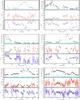 |
Fig. 4 Flux density excesses (flares) observed in NIR Ks-band polarimetry mode of Sgr A*. These events were observed on 2004 June 13, 2005 July 30, 2006 June 1, 2007 May 15, 2007 May 17, 2008 May 25, 2008 May 27, 2008 May 30, 2008 June 1, 2008 June 3, 2009 May 18, 2011 May 27, 2012 May 17 (the order of the images starts from top left to bottom right). In each panel: top: total flux density (black) and polarized flux density (cyan; polarization degree times total flux density) measured in mJy; middle: degree of linear polarization (red); bottom: polarization angle (blue). |
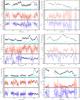 |
Fig. 4 continued. |
3. Data analysis
In Fig. 4 we show the light curves that represent all flaring activities observed in NIR Ks-band by NACO in polarization mode. Typical strong flux density excursions last for about 100 min. The changes in total flux density, polarization degree and polarization angle are more apparent when bright flare states occur. Although the flare events are different in terms of the maximum flux density, it is interesting to investigate if there are preferred values or ranges of values for the polarization degree and angle that are independent of the flare flux density.
The flux density uncertainties for our statistical analysis are determined via the relation shown in Fig. 3 and we use the results of our analysis presented in the following for determining the uncertainties of the polarization degree and angle.
3.1. Expected statistical behavior of polarization measurements
In order to adequately present and interpret the data we need to know what the expected statistical behavior of polarization measurements is. The polarization statistics has been studied by several authors, e.g. Serkowski (1958, 1962), Vinokur (1965), Simmons & Stewart (1985), Naghizadeh-Khouei & Clarke (1993), Clarke (2010). From Eq. (4)it is clear that the polarization degree p is a positive quantity that takes values between zero and one (or equivalently 0 − 100%). The uncertainties in Q and U, which in our case are the result of observational noise in the polarization channels, biases the value of p. This leads to an overestimation of p at low signal-to-noise (S/N) measurements. In general, polarimetric observations require a higher S/N compared to photometric measurements. To first order the S/N of the total intensity is related to that of the polarized intensity like (S/N)polarized intensity ≈ p × (S/N)total intensity, where the degree of polarization is usually smaller than one. As a result, weak polarization signal can be detected in case of having high (S/N)total intensity (Trippe 2014).
The polarization degree distribution does not follow a Gaussian distribution in the presence of random noise except for large S/N. In Sect. 2.1, we showed that total intensity measurements of stars around Sgr A* are, in very good approximation, Gaussian distributed; this means that the noise in the polarization channels must have the same distribution. Hence, U and Q follow Cauchy distributions that, at medium S/N, can already be approximated by normal distributions around the intrinsic values U0 and Q0. In this case, and assuming that U and Q are independent variables with associated variances equal to  , the polarization-degree distribution F(p;p0,σ0) for a particular value of the intrinsic polarization degree
  can be described by a Rice distribution,
 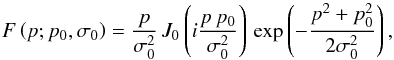 (6)where J0(ix) is the zero-order Bessel function of the imaginary argument (Serkowski 1958; Vinokur 1965). Simmons & Stewart (1985) studied the bias on the observed value of p for different (S/N)polarization degree defined as P0 = p0/σ0 (see their Fig. 1). The most probable observed value of p is the peak of the F(p;p0,σ0) distribution, which is always larger than p0 for low S/N, and approaches the intrinsic value p0 with increasing S/N. At low S/N, the polarization-angle distribution is multi-modal with a spread that covers the whole range of possible values of φ. At medium S/N and under the same assumptions as previously, the probability distribution F(φ;φ0,P0) for a particular intrinsic polarization angle φ0 is symmetric around its most probable value, and depends on the (S/N)polarization degree. It can be expressed as:
 ![Mathematical equation: \begin{equation} F(\phi; \phi_0, P_0) = \left\{ \frac{1}{\pi} + \frac{\eta_0 }{\sqrt{\pi}} \, {\rm e^{\eta_0^2}} \left[1+ {\rm erf}(\eta_0) \right] \right\} \, \exp{\left( -\frac{P_0^2}{2} \right)}, \end{equation}](/articles/aa/full_html/2015/04/aa25239-14/aa25239-14-eq44.png) (7)with
(7)with 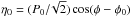 , and “erf” the Gaussian error function (Vinokur 1965; Naghizadeh-Khouei & Clarke 1993). When S/N is high, the distribution tends toward a Gaussian distribution with standard deviation
  (radians), where the dispersion in the polarization degree is σp = σ0 (Serkowski 1958, 1962). Simmons & Stewart (1985) and Stewart (1991) have proposed several methods to remove the bias in the observed p measurements for a source with a constant polarization state. However, whether this condition is fulfilled in the case of Sgr A* is unknown. Furthermore, there are scenarios that predict variability of its intrinsic polarization degree and angle. Therefore, without any a priori assumptions on the polarization properties of Sgr A*, it is necessary to follow the propagation of the uncertainties from the observables, measured quantities i.e. flux densities in the polarization channels, to the calculated polarization properties p and φ. We performed Monte Carlo simulations of the measured quantities and the observational noise, and used them to statistically analyze the calculated polarization degree and angle distributions and their uncertainties. The initial parameters of the simulation are the total flux density F0 and its uncertainty σF, and the intrinsic polarization degree p0 and angle φ0. For each set of these parameters, the corresponding polarization-channel fluxes f0,f90,f45, and f135 can be calculated from Eqs. (1)–(5). In order to associate an uncertainty with the flux measured in each polarization channel fX, we considered the relation between the total flux densities and their uncertainties presented in Sect. 2.1.
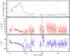 |
Fig. 4 continued. |
Given that the distributions of F are in a very good approximation Gaussian, and that the noise in each par of orthogonal polarization channels is about the same, then the standard deviation of the Gaussian function that describes the distribution of each fX can be expressed as  , i.e.
  . For each set (F0,p0,φ0), we draw from the fX distributions, 104 tetrads of polarization-channel fluxes and use them to calculate U, Q, p and φ, as it is done with real data. From the simulations it is possible to establish the most probable observed values of p and φ, as well as the ranges in which certain percentages of the values are contained. We consider intrinsic total flux densities ranging from 0.8 mJy, which is the photometry detection limit (Witzel et al. 2012), to 15.0 mJy, which is approximately the maximum value in our data set. The initial values for polarization degree (the amplitude of the intrinsic polarization, p0) are set to a range from 5% to 70%, while φ0 is fixed to a preferred polarization angle of 13°, based on the following data analysis. Figures 5 and 6 show the resulting distributions of U, Q, p and φ for two different initial total flux values, one with medium S/N and the other with high S/N, as an example. The distributions in the plots correspond to the values that an observer would measure for a source whose intrinsic total flux, polarization degree and polarization angle are the initial values given at beginning of the simulation. We use the limits of the intervals containing 68%, 95% and 99% of all values as our effective 1σ, 2σ and 3σ error intervals. This gives us asymmetric errors for p in the form
  . From these two examples it is clear that the most probable value of p is larger than its true value p0, but p becomes closer to p0 for higher S/N.
Moreover, we have fitted a Rice function to the p distribution and obtained the σ value of Rice distribution. Table 2 presents the simulated polarization degree values for different initial flux and polarization degree values. In the case of polarization angle, we have considered the confidence intervals and obtained σ values only if the S/N is larger than 4.5, since for the lower S/N, the φ distribution has a non-Gaussian shape. Table 2 presents the simulated polarization degree values for different initial flux and polarization degree values.
Figure 7 represents the relation between the simulated values of the total flux and the polarization degree. The contours shown in the figure correspond to 1σ, 2σ and 3σ values that enclose 68%, 95%, and 99% of points in the distribution, i.e. if the observer could measure these quantities more than 1000 times then, the central contour would enclose the 68% of measured values that are closest to the intrinsic value.
The following results of the expected statistical properties of our polarization data will be used for interpretation in the upcoming section.
From Fig. 5 and Table 2 one can see that for our NIR data for strong flare fluxes the recovered degree of polarization is Gaussian distributed around a very well central value close to the intrinsic degree with a ~5% uncertainty. Hence, if the intrinsic polarization degree is centered around a fixed expectation value the statistical properties of bright flare samples will be very similar to those of the total flux density measurements as presented by Witzel et al. (2012).
One can see from Fig. 5 and Table 2 that for weak intrinsic fluxes the recovered degree of polarization is not any longer Gaussian distributed and especially for moderate or weaker intrinsic polarization degrees the intrinsic value is not well recovered and the uncertainties are very large, such that unrealistic polarization degrees of above 100% can be obtained. The intrinsic polarization degrees are statistically recovered for intrinsically strongly polarized weak flares, but the un-symmetric uncertainties remain very large. Therefore, the total statistical behavior of observed polarization data can be thought of as being composed of the properties of subsamples of different polarization degrees and flare fluxes.
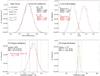 |
Fig. 5 Initial values for simulation: total flux = 6 mJy, polarization degree = 30% and polarization angle = 13°. |
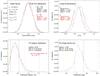 |
Fig. 6 Initial values for simulation: total flux = 1 mJy, polarization degree = 30% and polarization angle = 13°. |
Average values of recovered polarization degrees obtained by simulation for the combination of different sets of intrinsic total flux F′ and polarization degree p′ as initial values.
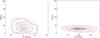 |
Fig. 7 Relation between simulated values of total flux density and polarization degree for initial values of: left: total flux = 1 mJy, polarization degree = 30%, polarization angle = 13°, right: total flux = 6 mJy, polarization degree = 30%, polarization angle = 13°. |
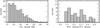 |
Fig. 8 Left: distribution of Ks-band polarization degrees of Sgr A* for our data set considering the significant data points (based on Table 2). Right: distribution of relative uncertainties of the polarization degrees. |
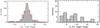 |
Fig. 9 Left: distribution of significant Ks-band polarization angles of Sgr A*. The red line shows the fit with a Gaussian distribution. Right: distribution of absolute errors of the polarization angles. |
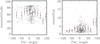 |
Fig. 10 Left: altitude (elevation) of Sgr A* as a function of polarization angle; Right: total flux density as a function of polarization angle; The bin width in polarization angle is 15°. The values for individual measurements are shown as black dots. The mean values per bin are shown as red dots with error bars indicating the standard deviation, if the number of data points per bin is larger than 2. |
3.2. Polarization degree and polarization angle
In Fig. 8 we show the distribution of Ks-band polarization degrees of Sgr A* (left) as well as the distribution of their uncertainties (right) obtained following the results of our statistical analysis presented in Sect. 3.1. In these figures we only plot the data points for which – based on our simulations – both the upper and lower uncertainty of the recovered polarization degree are smaller than half of the actual recovered value. In the following we will refer to these values as being significant measurements i.e. successful retrievals of the intrinsic polarization degree (and angle; see below).
The distribution of polarization degrees has a peak close to ~20%. It does not have the shape of a Gaussian and is strongly influenced by systematic effects with uncertainties ranging from 10% to 50% (see Sect. 3.1).
A Gaussian distribution would have been expected for the polarization degree if it had a single preferred value around which the realized and/or observed values then scatter. For our data set this is not the case. The fact that the distribution is not Gaussian shows that all degrees up to the highest expected values for synchrotron emission are realized by the responsible emission process. As shown later this is due to an underlying well-defined range of polarization degrees and limitations in the measuring process for weak flare fluxes.
Figure 9 shows the distribution of significant Ks-band polarization angles of Sgr A* (left) and their uncertainties (right) as determined for the corresponding flare fluxes following the statistical analysis presented in Sect. 3.1. For table entries with significant polarization degrees the corresponding uncertainties in the recovered polarization angle are below ±20° i.e. below about 1/3 of a radian. The distribution of polarization angles shows a peak at 13°. The overall width of the distribution is on the order of 30°, hence, the preferred polarization angle that we can derive from the distribution is 13° ± 15°. In Fig. 13 (right) we show for all data with significant polarization degrees the angle as a function of total flux density. The same plot for the entire data set is shown in Fig. A.4. The distribution of polarization angle and degree for the entire data set are shown in Fig. A.2.
The data shown on the left side of Figs. 8 and 9 are consistent in the sense that the uncertainty of Δφ = 15° in polarization angle is reflected in the width of the distribution of uncertainties derived from our simulations Fig. 8 (right). This implies that the uncertainty in angle is dominated by the measurement error and the physical variabilities of the angle is probably much smaller. The measurement error is the combined uncertainty of recording the data and retrieving the polarization information out of it. An upper limit for the uncertainties in polarization angles (Fig. 9, right) is Δφ = 20°. This value Δφ also implies a corresponding expected relative uncertainty of the polarization degree of about 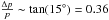 (i.e. 36%, for explanation see sketch in Fig. A.5). This is in good agreement with the approximate center value of 0.3 (i.e. 30%) found for the slightly skewed distribution of relative uncertainties of the polarization degree (Fig. 8, right) for the entire set of significant data as judged from the simulations. Since the uncertainty in angle only accounts for the lower portion of the distribution of relative uncertainties in polarization degree, this implies that the polarization degree is indeed dominated by intrinsic fluctuations of that quantity. Under the assumption that the measurement and intrinsic uncertainty add quadratically, the intrinsic variability of the relative 2 μm NIR polarization degree for Sgr A* is on the order of about 30%.
In order to investigate if the distribution of polarization angles of Sgr A* is affected by the strength of the flare and the position of this source in the sky, we plotted for all data with significant polarization degrees the average of flux densities versus the polarization angles binned in 15° intervals (Fig. 10, right) and the average elevation of Sgr A* in the sky for each polarization measurement (Fig. 10, left). The corresponding plots for all data are shown in Fig. A.1. The region in which a significant correction due to instrumental polarization needs to be applied is located at about ±0.5 h with respect to the meridian (see Fig. 9 in Witzel et al. 2011). This corresponds to an elevation of higher than about 80°. The distribution of data in Fig. 10 (left) indicates that most of the measurements were done at elevations below 75°, hence the correction for instrumental polarization is very small. The distribution of data in Fig. 10 (right) indicates for polarization angles close to the preferred angle of 13° the corresponding mean flux density is within about 1σ from the mean flux density values of all 15° intervals. Hence, the flux density values that correspond to polarization angles around the preferred value are not exceptionally high or low. In summary we can exclude that the preferred polarization angle of about 13° is related to flux density excursions of particular brightness or to a particular location in the sky and instrumental orientation. Therefore, we conclude that the preferred polarization angle is a source intrinsic property.
Except for measuring effects, the variable polarization of Sgr A* is source intrinsic. We point out that the stable foreground polarization in the central arcsecond is only on the order of 5% at 27 deg (Witzel et al. 2011) which agrees well with the value obtained for the over all central stellar cluster of 4% at 25 deg (Knacke & Capps 1977). These values show slow variations as a function of position due to the combination of foreground and the overall distribution of gas and dust in that region and the exception for individual dusty sources (Buchholz et al. 2013, 2011). The polarization degree during flares of Sgr A* is much stronger than that of the background and variable to a degree that show it is clearly source intrinsic.
3.3. Polarized flux density distribution
We produce the histogram of polarized flux density distribution of Sgr A* in its linear form (Fig. A.3, left) for the entire data and double logarithmic representation for the entire data (see Fig. A.3, right) as well as for the fraction of the data which is significant, based on our simulation, showed in Fig. 11. The distribution is normalized by the total number of points and bin size. We use the logarithmic histogram in order to better display the distribution of values (Fig. 11). In the following we present two different approaches to formally describe and physically explain the measured polarized flux density distribution shown in Fig. 11.
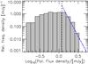 |
Fig. 11 Histogram of polarized flux density (total flux density times polarization degree) for all significant data in logarithmic scale after correction for stellar contamination. The thick black dashed line shows the position where the powerlaw starts to fit to the histogram. |
Average values of recovered polarization angles obtained by simulation for the combination of different sets of intrinsic total flux F′ and polarization degree p′ as initial values.
3.4. The polarized flux density distribution for bright flare fluxes
In Fig. 11 we show the histogram of polarized flux density. Our simulations have shown that only for bright flare fluxes can the polarization degree be recovered with a small uncertainty. Therefore, the properties of the polarized flux density distribution (i.e. the product of the polarization degree and the total flux density) can be investigated best for high polarized flare fluxes. A power-law fit to the data at high flux densities is shown as a dot-dashed blue line. For high flare fluxes the slope α is fitted to a value of 4.00 ± 0.15 which is very close to the value of 4.21 ± 0.05 obtained for the total flux densities by Witzel et al. (2012). The behavior was predicted by the simulations (see Fig. 5 and Table 2). Recovering this exponent for the polarized flare flux density distribution indicates that the intrinsic polarization degree is centered around a fixed expectation value (see Sect. 3.1) and has not been strongly variable over the time interval from 2004 to 2012.
3.5. A heuristic analytic explanation of the polarized flux density distribution
While the behavior of the entire sample of flares with significant polarized fluxes and polarization degrees is predicted by the simulations (see Figs. 5–7, and Tables 2 and 3, in Sect. 3.1), the heuristic model we present here helps us to understand the fact that the relative frequency density of measured polarized flux densities is much broader in comparison to the relative frequency density of total flux density measurements as presented by Witzel et al. (2012) which was found to be consistent with a single-state emission process.
In the following we call D(FK,pol) the relative frequency density of measured polarized flux densities as shown in Fig. 11. Keeping in mind the limited number of polarized flares that are available for our study this can be compared to the distribution shown for the total fluxes for a large sample of light curves by Witzel et al. (2012, see Fig. 3 therein). We now assume that for each randomly picked subset of Ks-band flux densities, total flux density distribution has a similar shape. We assume that for all flux densities all polarization degrees are possible. This assumption is not fully justified and we comment on this later. First, we pick values that belong to total flux densities SK that can be attributed to a polarization degree bin pi of width δp from pi − δp/2 to pi +δp/2 the polarized flux densities would be FK·pi. We obtain from the distribution shown in Fig. 8 (left) the weights wi(pi) for individual polarization states. We can express the polarized flux density distribution D(FK,pol) as a product distribution that is a probability distribution constructed as the distribution of the product of (assumed to be) independent random variables pi and D(FK) that have known distributions.
Using the weights wi(pi) for each polarization state the corresponding polarized flux density distribution D(FK,poli) can be written as  (8)The polarized flux density distribution D(FK,pol) can then be written as a product distribution by summing over all N bins including all polarization degrees pi:
  (9)In Fig. 12 we show the result of this modeling approach. In this figure we plot the measured (as in Fig. 11) and modeled relative number frequency of polarized flux density and show the combined contribution from different polarization states. The steep drop towards higher polarized flux densities is due to the deficiency of bright flares with high polarization states. Of course this region is also affected by the undersampling of the brightest flares. In this region our initial assumption that for all flux densities all polarization degrees are possible is not fulfilled. For fluxes above 5 mJy measured polarization degrees are below 30%. Therefore we overestimate the number of flare events with high polarized fluxes in this domain. Except this deficit, however, the model closely describes the measured data which implies that the broader distribution as formally analyzed in Sect. 3.3 can indeed be explained by combination of an intrinsic relative frequency total flux density histogram applied to the individual polarization states.
 |
Fig. 12 Relative number frequency of polarized flux density as derived from the light curves (Fig. 11) and from our heuristic modeling approach (straight red). The dashed curves show the contributions from flux densities with polarization degrees of ≤30% (blue), ≥60% (black) and in between (magenta). |
3.6. Relation between total flux density and polarization degree
Considering all the observed total flux densities for different epochs and their calculated polarization degrees, we plot the Ks-band polarization degrees versus total flux densities in Fig. 13 (left). In this figure we consider the data that result in significant measurements of polarization degrees i.e. we excluded data that correspond to positions shown in non bold face in Table 2. The same plot for the entire data set is shown in Fig. A.4. In both plots there is a clear trend that lower total flux densities have apparently higher polarization degrees, polarization degrees are lower for higher flux densities for which the simulations show that the polarization data can be recovered very well.
The boundary condition of detecting significant polarized flux density implies that the lower left, approximately triangular, region of any flux-polarization diagram remains empty. The detection limit for polarized flux is on the order of 0.3 mJy. The systematic uncertainty in the degree of polarization of about 5% is reflected in the systematic offset of 5% in the diagram. As we have shown in Table 2 the polarization degrees measured at low total fluxes show a much stronger, asymmetric, scatter than those obtained at higher total fluxes. This explains why the extension of the point cloud toward high values of p decreases with increasing total flux.
The apparent correlation is already implied by the results of the simulations (see Figs. 5, 6 and Table 2). Table 2 exhibits an apparent negative correlation between polarization degree and total flux density for intrinsic polarization degrees and total flux densities and it encloses the dashed line shown in Fig. 13 (left).
 |
Fig. 13 Left: relation between total flux density and polarization degree for significant data (based on Table 2). The dashed line shows the fitted line. Right: relation between total flux density and polarization angle for significant data. |
4. Discussion
4.1. Mechanisms that contribute to the polarization
Polarimetric observations can help to discriminate between different radiation mechanisms and source geometry. In case of active galactic nuclei, polarization over the range of spectral bands has been frequently employed to determine the structure of scattering regions (see e.g. Goosmann & Gaskell 2007) or to constrain the magnetic field in their accretion disks (Silant’ev et al. 2009). Preferred direction of polarization can help us to support or suppress the interpretation in terms of the synchrotron mechanism, which is thought to produce a particularly high polarization degree. Polarization perpendicular to the axis of symmetry is originating from scattering off material close to the axis or (as in the case of synchrotron emission) by the intrinsic emission mechanism. In this context often optical and UV observations are discussed, however, these are not particularly useful for Sgr A* and the investigation of the infrared polarization properties are therefore of special importance.
The rapid variability and the strong polarization imply that the emission from Sgr A* is dominated by synchrotron emission. In general the linear polarization is linked in degree and angle to the magnetic field structure and the source geometry. Hence measuring the polarization may allows us to evaluate the importance of various emission mechanisms. The situation for Sgr A* is complex. Neither is it clear if it has a permanent accretion disk nor is it clear if it has a permanent jet. All of these phenomena may occur as transients and come along with properties for the expected polarization degree and angle of the possible mechanisms. The Blandford-Znajek process (Blandford & Znajek 1977) permits the extraction of energy from a Kerr black hole. It results in a strong poloidal field, but requires an accretion disk to be present. Model calculations show that accretion disks may be dominated by ordered toroidal magnetic fields where the E-vector of the polarized radiation may be perpendicular to the equatorial plane (Broderick & Loeb 2006; Falcke & Markoff 2000; Goldston et al. 2005). However, magnetic field configurations in these systems can also be very turbulent (Shakura & Sunyaev 1973; Balbus & Hawley 1991). Hot spots within the disk may have a mostly vertical poloidal field structure (Eckart et al. 2006b) and may be coupled with reconnection events from magnetically arrested accretion disks (Dexter et al. 2014). In jet components the polarization vector can be perpendicular or parallel to the jet direction (Pollack et al. 2003; Gabuzda et al. 2000). In this context one should mention that Antonucci (1982) found that radio galaxies frequently exhibit a similar parallel alignment of the polarization and radio axes, but there is also a subclass showing a perpendicular direction.
However, there are also mechanisms that disturb characteristic polarization pattern. The polarization angle can be subject to projection effects (e.g. in the case of an inclined toroidal field) and can in addition be rotated in the strong gravitational field of the supermassive black hole if the line of sight to the emitting region passes close to it. Depolarization may occur as a result of this lensing effect in particular if complete or partial Einstein rings are formed. Depolarization may also occur if the source structure is complex. In both cases the polarization angles vary across the source and average out in larger beams. At NIR wavelengths strong depolarization due to the Faraday effect or Thompson scattering can be neglected. In future it is necessary to obtain structural information at a higher angular resolution to combine the information on polarization and source structure to allow for definitive conclusions on the importance of various mechanisms. With the current angular resolution and as a consequence of the situation described above one may expect that – within some uncertainties – the polarization angle of the emerging emission is either parallel or perpendicular to the emitting source structure.
4.2. Variable polarized flux
For the entire data set we find a large variation in polarization degree of – in part – larger than 50% and variations in flare flux density of >15 mJy.
However, simulations of the resulting observed polarization parameters given the measured flux (and its error) in orthogonal polarized channels show that, at low flux densities a significant part of the variation in polarization degree is due to measurement uncertainties. The simulations presented in Sect. 3.1 also show the uncertainty in recovering the intrinsic degree of polarization for flux levels above 5 mJy is only on the order of 5%. At this flux level, this value is considerably smaller than the measured variation in polarization degree at high fluxes of up to 30%. This implies an intrinsic variation of the polarization state of Sgr A* during flare events.
The defined range of polarization of 10−30% is lower than the maximum degree of polarization of about 70% that can be obtained for synchrotron radiation in tangled magnetic fields or a broad distribution of electron pitch angles with respect to the field lines (Moffet 1975; Ginzburg & Syrovatskii 1965). These high values are rarely observed as the polarization is spatially variable across the source and averaged in the observers beam. Hence it can be concluded that depolarization due to a complex source structure is at work.
For high fluxes the power-law slope of ~4 of the number density of the polarized flux density is very close to the slope in number density distribution of the total flux densities found by Witzel et al. (2012) which also clearly indicates that there is a preferred value or range of intrinsic degrees of polarization.
Finding this slope was unexpected as it is coupled to the previously unknown fact that the range of polarization degrees is limited to a small and well defined interval. As outlined in Witzel et al. (2012) the slope of the power-law flux density distribution implies a nonlinear statistical variability behavior of Sgr A* which is characterized by a linear rms-flux relation for the flux density range up to 12 mJy on a timescale of 24 min and a dominant timescale in that variability at about 150 min (Meyer et al. 2009).
The variation of this range of polarization degrees must have been small over the past years (2004–2012) else the slope in the number density of the polarized flux density would have been affected. Combined with the result from comparing the distributions of polarization degrees and their relative uncertainties this is a clear indication of intrinsic variability in the degree of polarization.
Consistent with this we derived in Sect. 3.2 for the entire set of significant polarization degrees its intrinsic relative variability must be on the order of 30%.
Therefore, the entire distribution of polarized flux density as described formally in Sect. 3.3 can be thought of as being composed of the contributions of populations of flare events with varying flux densities but a rather constant polarization angle and intrinsic polarization degrees that vary over a narrow range between about 10% and 30%. A preferred range in polarization degree and a well defined preferred polarization angle observed over a time span of 8 yr (2004–2012) supports the assumption of a rather stable geometry for the Sgr A* system, i.e. a rather stable disk and/or jet/wind orientation.
Comparison of polarization measurements of Sgr A* obtained in this paper with the ones reported in the literature.
In addition, a comparison of the observed data to the simulations presented in Sect. 3.1 shows that the observed anti-correlation between polarization degree and total flux density is most likely dominated by an observational effect due to asymmetrically distributed uncertainties in the determination of the polarization degree for small flare fluxes (close to our acceptance flux and below). This means that, with the current instrumentation, it is impossible to know whether the polarization state of Sgr A* is intrinsically variable at flux densities below 2 mJy. The observed apparent anti-correlation between polarization degree and total flux density means that the brighter flux density excursions are systematically less polarized than the lower flux densities. Such a behavior may be expected based on the findings by Zamaninasab et al. (2010) that the polarized flares in comparison with the randomly polarized red noise show a signature of radiating matter orbiting around the supermassive black hole. The formation of partial Einstein rings and mild relativistic boosting during the approach of an orbiting source component will lead to a bright geometrically depolarized emission during a flare event. Polarization variations caused by increasing or decreasing the flux densities have been reported in other publications (see e.g. Eckart et al. 2006b; Meyer et al. 2006a; Trippe et al. 2007).
It is also instructive to ensure that the results presented in this work are consistent with those of previous publications despite of different ways of extracting the polarization information. Table 4 presents a comparison of polarization angle and degree between this work and former NIR polarization studies of Sgr A*. Despite the strong source variability and different methods in deriving the observables (see Witzel et al. 2011, for details) the agreement is satisfactory and as expected from the findings in Sect. 3.5 and shown in Fig. 13.
4.3. The preferred polarization angle
We show that there is a preferred polarization angle of 13° ± 15° and that the polarized flux distribution is coupled to the total flux distribution analyzed in Witzel et al. (2012). The simulations presented in Sect. 3.1 show that the uncertainty in the polarization angle even at high flux levels (e.g. ≥5 mJy) is dominated by the statistical uncertainty (10° to 15°) in recovering a value that is assumed to be constant. Therefore, we can conclude that the intrinsic variability of the polarization angle is smaller than the currently measured variation and probably on the order of 10°.
However, in the discussion in Sect. 4.2 we now say: in general the variations are smaller if corrected for measuring uncertainties. However, looking at the plot of polarization angle versus flux density in Fig. 13 and the uncertainties expected for the angle, we find that for flare fluxes higher than 6 mJy (about 13% of the time; see Fig. 3 in Witzel et al. 2012) there are variations of the polarization angle in the range of 30° to 100° while the uncertainties are less than about 10° (see Tables 2 and 3). Hence there is a mixed behavior with a preferred polarization angle of about 13° for about 30% of the observing time at which the flare fluxes are above 2 mJy and clear excursions that cover a range much larger range than expected from observational/statistical uncertainties and clearly indicate the source intrinsic nature of the observed polarization of Sgr A*.
The preferred NIR polarization angle may also be linked to polarization properties in the radio cm- to mm-domain and to the orientation of the Sgr A* system. In the radio cm-regime linear polarization of Sgr A* is very small, however, the source shows a fractional circular polarization of around 0.4% (Bower et al. 1999b,a). The circular polarization decreases towards short mm-wavelengths (Bower et al. 2003), where Macquart et al. (2006) report a small percent of variable linear polarization from Sgr A* in the mm-domain. The polarization degree and angle in the sub-mm are likely linked to the magnetic field structure or the general orientation of the source. As in particular the NIR flare emission very likely originates from optically thin synchrotron radiation (Eckart et al. 2012) one may expect a link between the preferred NIR polarization angle and the NIR/radio structure of Sgr A*. At millimeter wavelengths interstellar scattering is small and allows insight into the intrinsic source structure of Sgr A*. Bower et al. (2014) report an intrinsic major axis position angle of the structure of 95° ± 10° (3σ). This angle of the radio structure is within the uncertainties orthogonal to the preferred infrared polarization angle. It is currently unclear how the intrinsic angle of Sgr A* can with certainty be related to external structures.
In a range of position angles between 120° and 130°Eckart et al. (2006b,c) report an elongated NIR feature, an elongated X-ray feature (see also Morris et al. 2004) and a more extended elongated structure called LF, XF, and EF in Fig. 9 by Eckart et al. (2006b). These features may be associated with a jet phenomenon. In this case the preferred NIR polarization angle may be associated with the jet components close to or at the foot point of the jet as for jet components the polarization may be along or perpendicular to the jet direction.
It is also possible that the NIR emission originates in hot spots on an accretion disk in a sunspot like geometry in which the E-vector is mainly perpendicular to the equatorial plane. Such a magneto-hydrodynamical model for the formation of episodic fast outflow is presented by Yuan et al. (2009). Acceleration of coronal plasma due to reconnection may then drive a jet or wind perpendicular to the intrinsic radio structure of the disk along the position angle of the NIR polarization. The mini-cavity that may be due to the interaction of a nuclear wind from Sgr A* is located at a position angle of about 193° (i.e. 13° + 180°). The cometary tails of sources X3 and X7 reported by Mužić et al. (2010) also present additional observational support for the presence of a fast wind from Sgr A* under that position angle.
5. Summary and conclusions
We have analyzed the NIR polarization light curves obtained with NACO at the ESO VLT for Sgr A* at the center of the Milky Way. Both the steep spectral index (Bremer et al. 2011, and references there in) and the strong variability in the NIR demonstrate that we are most likely dealing with optically thin synchrotron radiation (Eckart et al. 2012). Therefore, all properties we can derive based on the observation of variable polarized NIR radiation can directly be interpreted as source intrinsic properties. The main results can be summarized in the following points:
-
We estimate the expected uncertainties of the polarization degreeand angle of Sgr A* for the observed range of fluxdensities. Based on these expectations, we find that for fluxdensities >2 mJy Sgr A* shows intrinsic variability in polarization degree and angle. For low flare fluxes the polarization degree and angle are dominated by measuring uncertainties.
-
For flare fluxes above 5 mJy we find a range of polarization degrees of 10−30%. If the variable polarized flux from Sgr A* is due to optically thin synchrotron radiation this may indicate depolarization due to a spatially unresolved complex source structure.
-
There is a preferred variable polarization angle of 13° ± 15°. Corrected for the measuring uncertainties the intrinsic variability of Sgr A* is on the order of 10°. The angle may be linked to Jet/wind directions of the corresponding orientation of a temporary accretion disk.
-
For the number density of the polarized flux we find a power-law slope of ~4 which is very close to the slope in number density distribution of the total flux densities found by Witzel et al. (2012).
The well defined preferred ranges in polarization degree and angle as well as the number density power-law slope of 4 suggest that over the past 8 yr the geometry and accretion process for the Sgr A* system have been rather stable.
Further progress in investigating in particular the faint polarization states of Sgr A* in the NIR will require a higher angular resolution in order to better discriminate Sgr A* against background contamination. It is also of interest to use the well defined NIR polarization properties of Sgr A* to better determine the apparent stability of the underlying geometrical structure of the system and potentially use variations in this stability to trace interactions of the supermassive black hole at the center of the Milky Way with its immediate environment.
Online material
Appendix A
Here we provide additional plots similar to the ones shown throughout the main body of the text, showing the principal results from the analysis of Sgr A* observations taken in the polarization mode (NACO), but using the entire data set without limitation to the only significant values.
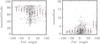 |
Fig. A.1 Left: altitude (elevation) of Sgr A* as a function of polarization angle as derived from all data. Right: total flux density as a function of polarization angle; the bin width in polarization angle is 15°. The values for individual measurements are shown as black dots. The mean values per bin are shown as red dots with error bars indicating the standard deviation, if the number of data points per bin is larger than 2. |
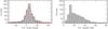 |
Fig. A.2 Left: distribution of Ks-band polarization angles of Sgr A* for the entire data set. The red line shows the fit with a Gaussian distribution. Right: distribution of Ks-band polarization degrees of Sgr A* for the entire data set. |
 |
Fig. A.3 Left: histogram of polarized flux density (total flux density times polarization degree) for the whole data set after correction for stellar contamination. Right: same plot in logarithmic scale. |
Comparison between the figures in the main text and those shown here in the Appendix allows the reader to get an impression of the effect of selecting the most significant values for the analysis presented.
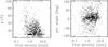 |
Fig. A.4 Left: total flux density and degree of polarization relation for the entire data after correction for the offset. Right: total flux density and angle of polarization relation for the entire data after correction for the offset. |
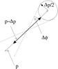 |
Fig. A.5 Approximate relation Δp ~ ptan(Δφ) between the mean uncertainty of the polarization angle Δφ and the polarization degree Δp. Here polarization degree p and polarization angle φ are projected on the sky. |
Acknowledgments
We would like to thank the anonymous referee for insightful comments that led to improvements in this paper. B.Sh. and N.S are members of the Bonn Cologne Graduate School (BCGS) for Physics and Astronomy supported by the Deutsche Forschungsgemeinschaft and acknowledge support from BCGS. B.Sh. gladly thanks E. Clausen-Brown, S. Trippe and M. Oshagh for fruitful discussions. We received funding from the European Union Seventh Framework Programme (FP7/2007-2013) under grant agreement No. 312789. This work was also supported in part by the Max Planck Society and the University of Cologne through the International Max Planck Research School (IMPRS) for Astronomy and Astrophysics. Part of this work was supported by the German Deutsche Forschungsgemeinschaft, DFG, via grant SFB 956 and fruitful discussions with members of the European Union funded COST Action MP0905: Black Holes in a violent Universe and the COST Action MP1104: Polarization as a tool to study the Solar System and beyond.
References
- Antonucci, R. R. J. 1982, Nature, 299, 605 [NASA ADS] [CrossRef] [Google Scholar]
- Baganoff, F. K., Bautz, M. W., Brandt, W. N., et al. 2001, Nature, 413, 45 [NASA ADS] [CrossRef] [PubMed] [Google Scholar]
- Balbus, S. A., & Hawley, J. F. 1991, ApJ, 376, 214 [NASA ADS] [CrossRef] [Google Scholar]
- Blandford, R. D., & Znajek, R. L. 1977, MNRAS, 179, 433 [NASA ADS] [CrossRef] [Google Scholar]
- Bower, G. C., Backer, D. C., Zhao, J.-H., Goss, M., & Falcke, H. 1999a, ApJ, 521, 582 [NASA ADS] [CrossRef] [Google Scholar]
- Bower, G. C., Falcke, H., & Backer, D. C. 1999b, ApJ, 523, L29 [NASA ADS] [CrossRef] [Google Scholar]
- Bower, G. C., Wright, M. C. H., Falcke, H., & Backer, D. C. 2003, ApJ, 588, 331 [NASA ADS] [CrossRef] [Google Scholar]
- Bower, G. C., Markoff, S., Brunthaler, A., et al. 2014, ApJ, 790, 1 [Google Scholar]
- Bremer, M., Witzel, G., Eckart, A., et al. 2011, A&A, 532, A26 [NASA ADS] [CrossRef] [EDP Sciences] [Google Scholar]
- Broderick, A. E., & Loeb, A. 2006, MNRAS, 367, 905 [NASA ADS] [CrossRef] [Google Scholar]
- Buchholz, R. M., Witzel, G., Schödel, R., et al. 2011, A&A, 534, A117 [NASA ADS] [CrossRef] [EDP Sciences] [Google Scholar]
- Buchholz, R. M., Witzel, G., Schödel, R., & Eckart, A. 2013, A&A, 557, A82 [NASA ADS] [CrossRef] [EDP Sciences] [Google Scholar]
- Chan, C.-K., Liu, S., Fryer, C. L., et al. 2009, ApJ, 701, 521 [NASA ADS] [CrossRef] [Google Scholar]
- Clarke, D. 2010, Stellar Polarimetry (Wiley) [Google Scholar]
- Devillard, N. 1999, in Astronomical Data Analysis Software and Systems VIII, eds. D. M. Mehringer, R. L. Plante, & D. A. Roberts, ASP Conf. Ser., 172, 333 [Google Scholar]
- Dexter, J., McKinney, J. C., Markoff, S., & Tchekhovskoy, A. 2014, MNRAS, 440, 2185 [NASA ADS] [CrossRef] [Google Scholar]
- Diolaiti, E., Bendinelli, O., Bonaccini, D., et al. 2000, A&AS, 147, 335 [NASA ADS] [CrossRef] [EDP Sciences] [Google Scholar]
- Do, T., Ghez, A. M., Morris, M. R., et al. 2009, ApJ, 691, 1021 [NASA ADS] [CrossRef] [Google Scholar]
- Dodds-Eden, K., Porquet, D., Trap, G., et al. 2009, ApJ, 698, 676 [NASA ADS] [CrossRef] [Google Scholar]
- Dodds-Eden, K., Gillessen, S., Fritz, T. K., et al. 2011, ApJ, 728, 37 [NASA ADS] [CrossRef] [Google Scholar]
- Doi, K. 1978, Nature, 275, 197 [NASA ADS] [CrossRef] [Google Scholar]
- Dovčiak, M., Karas, V., & Yaqoob, T. 2004, ApJS, 153, 205 [NASA ADS] [CrossRef] [Google Scholar]
- Dovčiak, M., Karas, V., Matt, G., & Goosmann, R. W. 2008, MNRAS, 384, 361 [NASA ADS] [CrossRef] [Google Scholar]
- Eckart, A., & Genzel, R. 1996, Nature, 383, 415 [NASA ADS] [CrossRef] [Google Scholar]
- Eckart, A., & Genzel, R. 1997, MNRAS, 284, 576 [NASA ADS] [Google Scholar]
- Eckart, A., Genzel, R., Ott, T., & Schödel, R. 2002, MNRAS, 331, 917 [NASA ADS] [CrossRef] [Google Scholar]
- Eckart, A., Baganoff, F. K., Morris, M., et al. 2004, A&A, 427, 1 [NASA ADS] [CrossRef] [EDP Sciences] [Google Scholar]
- Eckart, A., Baganoff, F. K., Schödel, R., et al. 2006a, A&A, 450, 535 [NASA ADS] [CrossRef] [EDP Sciences] [Google Scholar]
- Eckart, A., Schödel, R., Meyer, L., et al. 2006b, A&A, 455, 1 [Google Scholar]
- Eckart, A., Schodel, R., Meyer, L., et al. 2006c, J. Phys. Conf. Ser., 54, 391 [NASA ADS] [CrossRef] [Google Scholar]
- Eckart, A., Baganoff, F. K., Zamaninasab, M., et al. 2008a, A&A, 479, 625 [NASA ADS] [CrossRef] [EDP Sciences] [Google Scholar]
- Eckart, A., Schödel, R., García-Marín, M., et al. 2008b, A&A, 492, 337 [NASA ADS] [CrossRef] [EDP Sciences] [Google Scholar]
- Eckart, A., García-Marín, M., Vogel, S. N., et al. 2012, J. Phys. Conf. Ser., 372, 012022 [NASA ADS] [CrossRef] [Google Scholar]
- Eisenhauer, F., Schödel, R., Genzel, R., et al. 2003, ApJ, 597, L121 [NASA ADS] [CrossRef] [Google Scholar]
- Falcke, H., & Markoff, S. 2000, A&A, 362, 113 [NASA ADS] [Google Scholar]
- Gabuzda, D. C., Pushkarev, A. B., & Cawthorne, T. V. 2000, MNRAS, 319, 1109 [NASA ADS] [CrossRef] [Google Scholar]
- Genzel, R., Schödel, R., Ott, T., et al. 2003, Nature, 425, 934 [CrossRef] [PubMed] [Google Scholar]
- Ghez, A. M., Klein, B. L., Morris, M., & Becklin, E. E. 1998, ApJ, 509, 678 [NASA ADS] [CrossRef] [Google Scholar]
- Ghez, A. M., Morris, M., Becklin, E. E., Tanner, A., & Kremenek, T. 2000, Nature, 407, 349 [NASA ADS] [CrossRef] [PubMed] [Google Scholar]
- Ghez, A. M., Hornstein, S. D., Lu, J. R., et al. 2005, ApJ, 635, 1087 [NASA ADS] [CrossRef] [Google Scholar]
- Ghez, A. M., Salim, S., Weinberg, N. N., et al. 2008, ApJ, 689, 1044 [NASA ADS] [CrossRef] [Google Scholar]
- Gillessen, S., Eisenhauer, F., Quataert, E., et al. 2006, ApJ, 640, L163 [NASA ADS] [CrossRef] [Google Scholar]
- Gillessen, S., Eisenhauer, F., Trippe, S., et al. 2009, ApJ, 692, 1075 [NASA ADS] [CrossRef] [Google Scholar]
- Ginzburg, V. L., & Syrovatskii, S. I. 1965, ARA&A, 3, 297 [NASA ADS] [CrossRef] [Google Scholar]
- Goldston, J. E., Quataert, E., & Igumenshchev, I. V. 2005, ApJ, 621, 785 [NASA ADS] [CrossRef] [Google Scholar]
- Goosmann, R. W., & Gaskell, C. M. 2007, A&A, 465, 129 [NASA ADS] [CrossRef] [EDP Sciences] [Google Scholar]
- Hamaus, N., Paumard, T., Müller, T., et al. 2009, ApJ, 692, 902 [NASA ADS] [CrossRef] [Google Scholar]
- Knacke, R. F., & Capps, R. W. 1977, ApJ, 216, 271 [NASA ADS] [CrossRef] [Google Scholar]
- Lenzen, R., Hartung, M., Brandner, W., et al. 2003, in Instrument Design and Performance for Optical/Infrared Ground-based Telescopes, eds. M. Iye, & A. F. M. Moorwood, SPIE Conf. Ser., 4841, 944 [Google Scholar]
- Liu, S., Petrosian, V., Melia, F., & Fryer, C. L. 2006, ApJ, 648, 1020 [NASA ADS] [CrossRef] [Google Scholar]
- Lucy, L. B. 1974, AJ, 79, 745 [NASA ADS] [CrossRef] [Google Scholar]
- Macquart, J.-P., Bower, G. C., Wright, M. C. H., Backer, D. C., & Falcke, H. 2006, ApJ, 646, L111 [NASA ADS] [CrossRef] [Google Scholar]
- Markoff, S., Falcke, H., Yuan, F., & Biermann, P. L. 2001, A&A, 379, L13 [NASA ADS] [CrossRef] [EDP Sciences] [Google Scholar]
- Meyer, L., Eckart, A., Schödel, R., et al. 2006a, A&A, 460, 15 [NASA ADS] [CrossRef] [EDP Sciences] [Google Scholar]
- Meyer, L., Schödel, R., Eckart, A., et al. 2006b, A&A, 458, L25 [NASA ADS] [CrossRef] [EDP Sciences] [Google Scholar]
- Meyer, L., Schödel, R., Eckart, A., et al. 2007, A&A, 473, 707 [NASA ADS] [CrossRef] [EDP Sciences] [Google Scholar]
- Meyer, L., Witzel, G., Longstaff, F. A., & Ghez, A. M. 2014, ApJ, 791, 24 [NASA ADS] [CrossRef] [Google Scholar]
- Moffet, A. T. 1975, Strong Nonthermal Radio Emission from Galaxies, eds. A. Sandage, M. Sandage, & J. Kristian (The University of Chicago Press), 211 [Google Scholar]
- Morris, M., Howard, C., Muno, M., et al. 2004, in The Dense Interstellar Medium in Galaxies, eds. S. Pfalzner, C. Kramer, C. Staubmeier, & A. Heithausen, 281 [Google Scholar]
- Mužić, K., Eckart, A., Schödel, R., et al. 2010, A&A, 521, A13 [NASA ADS] [CrossRef] [EDP Sciences] [Google Scholar]
- Naghizadeh-Khouei, J., & Clarke, D. 1993, A&A, 274, 968 [NASA ADS] [Google Scholar]
- Ott, T., Eckart, A., & Genzel, R. 1999, ApJ, 523, 248 [NASA ADS] [CrossRef] [Google Scholar]
- Pineault, S. 1980, ApJ, 241, 528 [NASA ADS] [CrossRef] [Google Scholar]
- Pollack, L. K., Taylor, G. B., & Zavala, R. T. 2003, ApJ, 589, 733 [NASA ADS] [CrossRef] [Google Scholar]
- Porquet, D., Predehl, P., Aschenbach, B., et al. 2003, A&A, 407, L17 [NASA ADS] [CrossRef] [EDP Sciences] [Google Scholar]
- Richardson, R. 1972, JOSA, 62, 55 [Google Scholar]
- Rousset, G., Lacombe, F., Puget, P., et al. 2003, in Adaptive Optical System Technologies II, eds. P. L. Wizinowich & D. Bonaccini, SPIE Conf. Ser., 4839, 140 [Google Scholar]
- Sabha, N., Witzel, G., Eckart, A., et al. 2010, A&A, 512, A2 [NASA ADS] [CrossRef] [EDP Sciences] [Google Scholar]
- Sabha, N., Eckart, A., Merritt, D., et al. 2012, A&A, 545, A70 [NASA ADS] [CrossRef] [EDP Sciences] [Google Scholar]
- Schödel, R., Ott, T., Genzel, R., et al. 2002, Nature, 419, 694 [NASA ADS] [CrossRef] [PubMed] [Google Scholar]
- Schödel, R., Najarro, F., Muzic, K., & Eckart, A. 2010, A&A, 511, A18 [NASA ADS] [CrossRef] [EDP Sciences] [Google Scholar]
- Serkowski, K. 1958, Acta Astron., 8, 135 [NASA ADS] [Google Scholar]
- Serkowski, K. 1962, Adv. Astron. Astrophys., 1, 289 [NASA ADS] [CrossRef] [Google Scholar]
- Shakura, N. I., & Sunyaev, R. A. 1973, A&A, 24, 337 [NASA ADS] [Google Scholar]
- Silant’ev, N. A., Piotrovich, M. Y., Gnedin, Y. N., & Natsvlishvili, T. M. 2009, A&A, 507, 171 [NASA ADS] [CrossRef] [EDP Sciences] [Google Scholar]
- Simmons, J. F. L., & Stewart, B. G. 1985, A&A, 142, 100 [NASA ADS] [Google Scholar]
- Stewart, B. G. 1991, A&A, 246, 280 [NASA ADS] [Google Scholar]
- Trippe, S. 2014, J. Kor. Astron. Soc., 47, 15 [Google Scholar]
- Trippe, S., Paumard, T., Ott, T., et al. 2007, MNRAS, 375, 764 [NASA ADS] [CrossRef] [Google Scholar]
- Vinokur, M. 1965, Ann. Astrophys., 28, 412 [NASA ADS] [Google Scholar]
- Witzel, G., Eckart, A., Buchholz, R. M., et al. 2011, A&A, 525, A130 [NASA ADS] [CrossRef] [EDP Sciences] [Google Scholar]
- Witzel, G., Eckart, A., Bremer, M., et al. 2012, ApJS, 203, 18 [NASA ADS] [CrossRef] [Google Scholar]
- Yuan, F., Quataert, E., & Narayan, R. 2004, ApJ, 606, 894 [NASA ADS] [CrossRef] [Google Scholar]
- Yuan, F., Lin, J., Wu, K., & Ho, L. C. 2009, MNRAS, 395, 2183 [NASA ADS] [CrossRef] [Google Scholar]
- Yusef-Zadeh, F., Bushouse, H., Dowell, C. D., et al. 2006a, ApJ, 644, 198 [NASA ADS] [CrossRef] [Google Scholar]
- Yusef-Zadeh, F., Roberts, D., Wardle, M., Heinke, C. O., & Bower, G. C. 2006b, ApJ, 650, 189 [NASA ADS] [CrossRef] [Google Scholar]
- Yusef-Zadeh, F., Wardle, M., Cotton, W. D., Heinke, C. O., & Roberts, D. A. 2007, ApJ, 668, L47 [NASA ADS] [CrossRef] [Google Scholar]
- Yusef-Zadeh, F., Wardle, M., Heinke, C., et al. 2008, ApJ, 682, 361 [NASA ADS] [CrossRef] [Google Scholar]
- Yusef-Zadeh, F., Bushouse, H., Wardle, M., et al. 2009, ApJ, 706, 348 [NASA ADS] [CrossRef] [Google Scholar]
- Zamaninasab, M., Eckart, A., Meyer, L., et al. 2008, J. Phys. Conf. Ser., 131, 012008 [NASA ADS] [CrossRef] [Google Scholar]
- Zamaninasab, M., Eckart, A., Witzel, G., et al. 2010, A&A, 510, A3 [NASA ADS] [CrossRef] [EDP Sciences] [Google Scholar]
All Tables
Average values of recovered polarization degrees obtained by simulation for the combination of different sets of intrinsic total flux F′ and polarization degree p′ as initial values.
Average values of recovered polarization angles obtained by simulation for the combination of different sets of intrinsic total flux F′ and polarization degree p′ as initial values.
Comparison of polarization measurements of Sgr A* obtained in this paper with the ones reported in the literature.
All Figures
|
Fig. 1 NIR Ks-band (2.2 μm) light curves of Sgr A* observed in polarimetry mode on 27 May 2011 (top) and 17 May 2012 (bottom) produced by combining pairs of orthogonal polarization channels; left: 0°, 90° and right: 45°, 135°. The blue dots show Sgr A* flux density measured in mJy, while the red connected dots show the background flux densities. |
| In the text | |
|
Fig. 2 Ks-band deconvolved image of the GC on 17 May 2012 showing the positions of Sgr A*, calibration stars and comparison apertures for background estimates marked by yellow circles. |
| In the text | |
|
Fig. 3 Top: normalized flux density distributions of 10 flux calibrators of Sgr A*. The dashed lines are Gaussian fits to the distributions. Bottom: standard deviation of flux densities of calibration stars versus flux densities of them. The red line is the polynomial fit to the measured σ values of the calibrators shown in the upper panel (red crosses). The two purple x symbols present the measured error values (obtained by Witzel et al. 2012) at the position of the comparison apertures for the background emission close to the position of Sgr A* (see Fig. 2). |
| In the text | |
|
Fig. 4 Flux density excesses (flares) observed in NIR Ks-band polarimetry mode of Sgr A*. These events were observed on 2004 June 13, 2005 July 30, 2006 June 1, 2007 May 15, 2007 May 17, 2008 May 25, 2008 May 27, 2008 May 30, 2008 June 1, 2008 June 3, 2009 May 18, 2011 May 27, 2012 May 17 (the order of the images starts from top left to bottom right). In each panel: top: total flux density (black) and polarized flux density (cyan; polarization degree times total flux density) measured in mJy; middle: degree of linear polarization (red); bottom: polarization angle (blue). |
| In the text | |
|
Fig. 4 continued. |
| In the text | |
|
Fig. 4 continued. |
| In the text | |
|
Fig. 5 Initial values for simulation: total flux = 6 mJy, polarization degree = 30% and polarization angle = 13°. |
| In the text | |
|
Fig. 6 Initial values for simulation: total flux = 1 mJy, polarization degree = 30% and polarization angle = 13°. |
| In the text | |
|
Fig. 7 Relation between simulated values of total flux density and polarization degree for initial values of: left: total flux = 1 mJy, polarization degree = 30%, polarization angle = 13°, right: total flux = 6 mJy, polarization degree = 30%, polarization angle = 13°. |
| In the text | |
|
Fig. 8 Left: distribution of Ks-band polarization degrees of Sgr A* for our data set considering the significant data points (based on Table 2). Right: distribution of relative uncertainties of the polarization degrees. |
| In the text | |
|
Fig. 9 Left: distribution of significant Ks-band polarization angles of Sgr A*. The red line shows the fit with a Gaussian distribution. Right: distribution of absolute errors of the polarization angles. |
| In the text | |
|
Fig. 10 Left: altitude (elevation) of Sgr A* as a function of polarization angle; Right: total flux density as a function of polarization angle; The bin width in polarization angle is 15°. The values for individual measurements are shown as black dots. The mean values per bin are shown as red dots with error bars indicating the standard deviation, if the number of data points per bin is larger than 2. |
| In the text | |
|
Fig. 11 Histogram of polarized flux density (total flux density times polarization degree) for all significant data in logarithmic scale after correction for stellar contamination. The thick black dashed line shows the position where the powerlaw starts to fit to the histogram. |
| In the text | |
|
Fig. 12 Relative number frequency of polarized flux density as derived from the light curves (Fig. 11) and from our heuristic modeling approach (straight red). The dashed curves show the contributions from flux densities with polarization degrees of ≤30% (blue), ≥60% (black) and in between (magenta). |
| In the text | |
|
Fig. 13 Left: relation between total flux density and polarization degree for significant data (based on Table 2). The dashed line shows the fitted line. Right: relation between total flux density and polarization angle for significant data. |
| In the text | |
|
Fig. A.1 Left: altitude (elevation) of Sgr A* as a function of polarization angle as derived from all data. Right: total flux density as a function of polarization angle; the bin width in polarization angle is 15°. The values for individual measurements are shown as black dots. The mean values per bin are shown as red dots with error bars indicating the standard deviation, if the number of data points per bin is larger than 2. |
| In the text | |
|
Fig. A.2 Left: distribution of Ks-band polarization angles of Sgr A* for the entire data set. The red line shows the fit with a Gaussian distribution. Right: distribution of Ks-band polarization degrees of Sgr A* for the entire data set. |
| In the text | |
|
Fig. A.3 Left: histogram of polarized flux density (total flux density times polarization degree) for the whole data set after correction for stellar contamination. Right: same plot in logarithmic scale. |
| In the text | |
|
Fig. A.4 Left: total flux density and degree of polarization relation for the entire data after correction for the offset. Right: total flux density and angle of polarization relation for the entire data after correction for the offset. |
| In the text | |
|
Fig. A.5 Approximate relation Δp ~ ptan(Δφ) between the mean uncertainty of the polarization angle Δφ and the polarization degree Δp. Here polarization degree p and polarization angle φ are projected on the sky. |
| In the text | |
Current usage metrics show cumulative count of Article Views (full-text article views including HTML views, PDF and ePub downloads, according to the available data) and Abstracts Views on Vision4Press platform.
Data correspond to usage on the plateform after 2015. The current usage metrics is available 48-96 hours after online publication and is updated daily on week days.
Initial download of the metrics may take a while.