| Issue |
A&A
Volume 576, April 2015
|
|
|---|---|---|
| Article Number | L6 | |
| Number of page(s) | 5 | |
| Section | Letters | |
| DOI | https://doi.org/10.1051/0004-6361/201425038 | |
| Published online | 23 March 2015 | |
Passive galaxies as tracers of cluster environments at z ~ 2
1 Irfu/Service d’Astrophysique, CEA Saclay, Orme des Merisiers, 91191 Gif-sur-Yvette, France
2 Department of Physics, Ludwig-Maximilians-Universität, Scheinerstr. 1, 81679 München, Germany
e-mail: vstrazz@usm.lmu.de
3 INAF−IASF, via Bassini 15, 20133 Milano, Italy
4 INAF−Osservatorio Astronomico di Bologna, via Ranzani 1, 40127 Bologna, Italy
5 Institute for Astronomy, ETH Zürich, Wolfgang-Pauli-strasse 27, 8093 Zürich, Switzerland
6 INAF-Osservatorio Astronomico di Padova, Vicolo dell’Osservatorio 5, 35122 Padova, Italy
7 Dipartimento di Fisica e Astronomia, Universitá di Bologna, Viale Berti Pichat 6/2, 30127 Bologna, Italy
8 Department of Physics, University of Helsinki, Gustaf Hällströmin katu 2a, 0014 Helsinki, Finland
9 National Astronomical Observatory of Japan, Subaru Telescope, 650 North Aohoku Place, Hilo, HI 96720, USA
10 Department of Physics, University of Oxford, Denys Wilkinson Building, Keble Road, Oxford, OX1 3RH, UK
11 IRAM−Institut de Radioastronomie Millimétrique, 300 rue de la Piscine, 38406 Saint-Martin dHères, France
12 Institut dAstrophysique de Paris, UMR 7095 CNRS, Université Pierre et Marie Curie, 75005 Paris, France
Received: 22 September 2014
Accepted: 17 January 2015
Even 10 billion years ago, the cores of the first galaxy clusters are often found to host a characteristic population of massive galaxies with already suppressed star formation. Here we search for distant cluster candidates at z ~ 2 using massive passive galaxies as tracers. With a sample of ~40 spectroscopically confirmed passive galaxies at 1.3 < z < 2.1, we tuned photometric redshifts of several thousand passive sources in the 2 sq. deg COSMOS field. This allowed us to map their density in redshift slices, probing the large-scale structure in the COSMOS field as traced by passive sources. We report here on the three strongest passive galaxy overdensities that we identify in the range 1.5 < z < 2.5. While the actual nature of these concentrations still needs to be confirmed, we discuss their identification procedure and the arguments supporting them as candidate galaxy clusters (probably in the mid-1013 M⊙ range). Although this search approach is probably biased toward more evolved structures, it has the potential of selecting still rare, cluster-like environments close to their epoch of first appearance, enabling new investigations of the evolution of galaxies in the context of structure growth.
Key words: galaxies: clusters: general / galaxies: high-redshift / large-scale structure of Universe
© ESO, 2015
1. Introduction
Up to at least z ~ 1, passive galaxies with typically early-type morphology dominate the high-mass end of the galaxy population and are the best tracers of the highest density peaks in the large-scale structure. The evolution of passive galaxy populations at z ≲ 1 – and in particular with respect to environmental effects – has also been explored in detail thanks to large spectroscopic campaigns (e.g., Kauffmann et al. 2004; Bernardi et al. 2006; Gallazzi et al. 2006, 2014; van der Wel et al. 2008; Sánchez-Blázquez et al. 2009; Kovač et al. 2014; Valentinuzzi et al. 2011; Muzzin et al. 2012). On the other hand, the spectroscopy of passive galaxies at z ≳ 1.5 has been until recently very difficult. In spite of several investigations pushing spectroscopic confirmation and more detailed studies to higher redshifts (e.g., Cimatti et al. 2004, 2008; Daddi et al. 2005; Kriek et al. 2006, 2009; Onodera et al. 2012; van de Sande et al. 2011, 2013; Toft et al. 2012; Gobat et al. 2012, 2013; Brammer et al. 2012; Weiner 2012; Krogager et al. 2014; Newman et al. 2014; Belli et al. 2014), sizable spectroscopic samples are still rare, and studying z> 1.5 passive populations mainly relies on photometric samples (e.g., Wuyts et al. 2010; Bell et al. 2012; Ilbert et al. 2013; Muzzin et al. 2013a; Cassata et al. 2013). These studies show that the number density of passive galaxies rapidly falls beyond z> 1, so that by z ~ 2 passive sources are no longer the dominant population, even among massive galaxies. However, the observed evolution of massive cluster galaxies up to z ~ 1 (and also theoretical models, e.g., De Lucia et al. 2006) typically suggests early (z ≳ 2 − 3) formation epochs for their stellar populations (e.g., Mei et al. 2009; Mancone et al. 2010; Strazzullo et al. 2010). We might thus expect that the surge in passive galaxies around ten billion years ago occurred differently in different environments.
Several recent studies have claimed to find evidence of significant star formation even in central cluster regions at z ≳ 1.5 (e.g., Hilton et al. 2010; Tran et al. 2010; Hayashi et al. 2010; Santos et al. 2011; Fassbender et al. 2011; Brodwin et al. 2013), suggesting that we indeed are approaching the formation epoch of massive cluster galaxies. However, it is also noticeable that massive passive galaxies are often found, even in such most distant clusters, although in many cases sharing their environment with galaxies in a still active formation phase (e.g., Kurk et al. 2009; Papovich et al. 2010; Gobat et al. 2011, 2013; Tanaka et al. 2013; Spitler et al. 2012; Strazzullo et al. 2013; Newman et al. 2014; Andreon et al. 2014). This may suggest that, even at a cosmic time when star formation rate density is at its peak (e.g., Madau & Dickinson 2014) and star formation is still active in a considerable fraction of massive galaxies (e.g., Ilbert et al. 2013; Muzzin et al. 2013a), the densest cores of most evolved cluster progenitors already host a typically small but characteristic population of massive quiescent galaxies. For this reason, overdensities of passive sources might be considered as possible signposts to clusters up at least to z ~ 2.
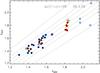 |
Fig. 1 Comparison of zphot vs. zspec for the full spectroscopic sample of 1.3 <z< 2.1 passive galaxies. Lower quality zspec determinations are shown in gray. Blue and red circles mark sources from the VIMOS and O12 samples, respectively. Orange stars highlight MIPS-detected sources. Dotted and solid lines show the bisector and a relative scatter of 2.5, 5, 10%. |
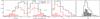 |
Fig. 2 Distributions of K-band magnitude, stellar mass and photometric redshift for the sample of KAB< 23, z> 1.3 passive galaxies. Three leftmost panels: full sample (see text, black line), its pBzK subsample (red line), and the spectroscopic sample (scaled by × 10, red shaded area). Vertical dotted lines show the magnitude and mass (at z< 2.5) completeness limits of the parent K-selected catalog (see text). Rightmost panel: full photo-z distribution of the KAB< 23 passive sample (black line), and of its log(M/M⊙) > 10.9 subsample (shaded area, lighter gray at z> 2.5 where sample is beyond mass completeness). |
2. Photometric redshift estimation for high-redshift passive galaxies in the COSMOS field
Using one of the first sizable samples of z ≳ 1.4 passive galaxies in the COSMOS field for calibration, in Onodera et al. (2012; hereafter O12) we could estimate more accurate photometric redshifts (photo-zs, zphot) for high-redshift passive sources. We have now assembled a new, independent sample of passive galaxies in COSMOS with redshifts measured through UV features using VLT/VIMOS spectroscopy. We targeted 29 IAB< 25 galaxies selected as passive BzKs (“pBzKs”, Daddi et al. 2004, plus 624 μm-detected pBzKs) from the McCracken et al. (2010; hereafter M10) catalog. A redshift was measured for 34 of the 35 targets, with a robust estimate for 29 sources. The observations, analysis, and a full redshift list will be presented in Gobat et al. (in prep.). Here we focus on a subsample of 42 spectroscopically confirmed pBzKs, selected in the range 1.3 <zspec< 2.1 and with restframe UVJ colors (Williams et al. 2009) consistent with passive populations (15 and 27 galaxies from the O12 and VIMOS samples, respectively, including 324 μm-detected sources as noted below). Figure 1 shows the performance on this sample of our photo-zs, estimated with EAzY (Brammer et al. 2008) and calibrated as in O12. The normalized median absolute deviation (NMAD) of Δz/ (1 + z) is 2.5% on the full sample, or 1.8% excluding galaxies with less reliable zspec (Fig. 1), with no catastrophic outliers (thus <2.5% for this sample). All results presented here are based on the photometric catalog by M101.
3. Passive galaxy overdensities at z > 1.5
Spectroscopic confirmation of large passive galaxy samples at high redshift is precluded for now, so we rely on passive candidates with photo-zs calibrated as above. We select a sample of z> 1.5 passive galaxies as follows: with an initial BzK selection on the M10 KAB< 23 catalog, we take all pBzK galaxies, as well as galaxies formally classified as star-forming BzKs (“sBzKs”) but with S/N< 5 in the B- (and possibly z-) band. From this first selection, we retain all galaxies also having UVJ passive colors (assuming their zphot as of Sect. 2). Sources detected at 24 μm and satisfying the above criteria are retained, because of the possibility of AGN-powered 24 μm flux. Sources with possibly contaminated IRAC photometry (as in the M10 catalog) were discarded (<10%). Figure 2 shows the stellar mass, K-band magnitude, and photo-z distributions for the full retained sample of passive galaxies and for its subsample of pBzK sources.
The KAB< 23 limit corresponds to 90% completeness for point-like sources, going down to ~22.5 for disk-like profiles (see M10). At z ~ 2.5, this translates in a mass completeness of log(M/M⊙) ~10.8−11 (~10.9 in the following, Salpeter 1955, IMF) for an unreddened SSP (Bruzual & Charlot 2003) of solar metallicity formed at z = 5. On the other hand, the combination of selection criteria adopted above is expected to result in a largely pure (in terms of contaminants) but not complete sample of massive (log(M/M⊙) ≳ 10.9) passive galaxies. For this reason, we may be missing some overdensities or reducing their significance, which would affect the results presented here in a conservative way. The BzK selection and the depth of the M10 catalog effectively limit our sample at z> 1.5 and z< 2.5, respectively (Fig. 2, right). The full sample of KAB< 23 passive galaxy candidates includes ~4500 sources. Of these, ~3500 are at 1.5 ≤ zphot ≤ 2.5 (~70% at log(M/M⊙) > 10.9, ~50% selected as pBzK, ~10% 24 μm-detected).
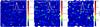 |
Fig. 3 Examples of Σ5 maps in redshift slices of the full passive galaxy sample in the 2 sq. deg COSMOS field (North is up, East is left). Maps are scaled so that red colors correspond to > 5σ significance. The three candidate overdensities described in Sect. 3.1 are highlighted with white circles (2 Mpc radius proper). In each plot, the inset shows the distribution of log(Σ5) values in the map and its Gaussian fit (white and orange lines, respectively), and the white arrow shows the peak Σ5 value of the highlighted overdensity. |
3.1. Identification of cluster candidates
We have built local density maps for the full COSMOS field in redshift slices, based on the catalog of passive galaxy candidates described above. In spite of the quoted ~2% photo-z relative accuracy (by comparison with zspec, Sect. 2), we need to consider that the spectroscopic sample is very biased toward brighter, lower redshift sources (Fig. 2), thus photo-z performance on the bulk of our sample is likely to be significantly worse. We estimated a more realistic photo-z accuracy as a function of magnitude, recalculating photo-zs on SEDs of well-fitted spectroscopic sources (| Δz|/(1 + z) < 2.5%) dimmed to fainter magnitudes, randomly scattering fluxes in the different bands according to photometric errors in our catalog. This simulation indeed gives a photo-z accuracy <2.5% at KAB ≲ 21 (Sect. 2), but rising to ~3.5% (5%) at KAB ~ 22 (22.5) and to more than 6% approaching our KAB ~ 23 limit. These estimates are “model-independent” in the sense that they use observed (rather than synthetic) SEDs, but they still assume that SEDs of less massive and/or higher redshift sources in our sample behave similarly to those of the spectroscopic sources used as input in the simulation. For comparison, the formal 68% errors estimated by EAzY on the simulated SEDs would be 40−50% larger on average (reaching ~8% at KAB ~ 23). For this reason, we built our density maps in redshift slices of Δz = ± 0.2 (corresponding to a ±1σ relative accuracy of 6−8% at 1.5 <z< 2.5) with a step of 0.05 in central redshift.
We used the Σ5 (5th nearest neighbor) density estimator, probing for our sample a median (over the full map) distance of ~1.4 Mpc in the z ~ 2 slice, with minimum and maximum distances of 100−200 kpc and 4−5 Mpc in all redshift slices, thus properly probing the typical scales we are investigating. For comparison, a Σ3 estimator would also probe such scales (median distance ~1.1 Mpc at z ~ 2, minimum and maximum distances ~50 kpc and 3−4 Mpc), while Σ7 would probe median distances closer to 2 Mpc with minimum/maximum of 0.5/4.5 Mpc at z ~ 2, thus becoming less sensitive to the scales we need to probe. Figure 3 shows three examples of Σ5 maps. For each map, we estimated the significance of overdensities by fitting the distribution of log(Σ5) in the whole map with a Gaussian (Fig. 3).
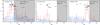 |
Fig. 4 Photo-z distributions for the whole (passive and star-forming) population of log(M/M⊙) > 10.9 galaxies within an aperture of r< 600 kpc from the three passive overdensities as labeled (red lines, errors as from Gehrels 1986). Galaxies and photo-zs used here are from Muzzin et al. (2013b) for CC1003+0223 and CC0958+0158, and from Ilbert et al. (2009) for CC1002+0134 (see text). In each panel, the blue line and dotted area show the median and 16th−84th percentiles of the photo-z distribution (from the same catalogs) in r< 600 kpc apertures at 100 random positions in the COSMOS field, while the grayed-out region shows the redshift range where the sample is no longer mass-complete. Black filled (empty) circles scattered above the histograms (at random y-axis coordinates) show our photo-z determinations for the passive sample used in this work within 300 kpc (600 kpc) from the overdensity center (larger/smaller symbols show galaxies more/less massive than log(M/M⊙) = 10.9). |
At the same time, we also used an independent approach to search for concentrations of massive passive galaxies with consistent photo-zs in a very small cluster-core sized area. In particular, based on observations of the z = 2 cluster Cl J1449+0857 (Gobat et al. 2011, 2013; Strazzullo et al. 2013, other examples in Sect. 1), we searched our log(M/M⊙) > 10.9 passive sample for sources with at least three other passive galaxies within | Δz |/(1 + z) < 7.5% (accounting for photo-z uncertainties described above) and a physical distance ≤150 kpc2. This approach independently retrieves the three most significant (≳7σ in the Σ5− as well as Σ3− maps) overdensities highlighted in Fig. 3:
-
CC1002+0134 at 1.5 ≲ zphot ≲ 1.8 – A concentration of passive sources around RA, Dec ~ 10h02m40s, + 01°34m20s, with four galaxies within a radius r = 90 kpc and zphot within ≤1.5σ (given each source magnitude, based on the simulation described above) from a mean zphot ~ 1.76. However, the photo-z distribution of the central sources in this candidate overdensity is quite broad compared to the expected photo-z uncertainties (see Fig. 4). This might suggest a chance superposition of passive galaxies or possibly of different, unrelated structures, along the line of sight at 1.5 <z< 1.8. On the other hand, Aravena et al. (2012) already reported the identification of a candidate cluster at zphot ~ 1.55 at the same position, based on an overdensity of galaxies with 1.5 <zphot< 1.6, a radio source at a consistent redshift, a tentative detection of extended X-ray emission, and the presence of a small population of passive sources. The actual nature of this structure is thus still unclear.
-
CC1003+0223 at zphot ~ 1.90 – A concentration of four passive galaxies at RA, Dec ~ 10h03m05s, + 02°23m24s within r< 110 kpc and zphot within ≲1.4σ from the mean zphot (another galaxy with zphot consistent within 1σ is found at r< 340 kpc). Half of these four sources were selected as UVJ-passive sBzKs (see Sect. 3). None is 24 μm-detected. All are consistent with also being UVJ-passive in the Muzzin et al. (2013b) catalog, three out of four with a photo-z consistent within 1σ with the mean zphot estimated here. The redshift distribution of the central sources is consistent with the presence of a single structure. Another overdensity of similar significance at a consistent photo-z is visible in the Σ5 map at <4 Mpc West (Fig. 3).
-
CC0958+0158 at zphot ~ 2.35− A concentration of four passive galaxies at RA, Dec ~ 9h58m53s,+ 01°58m01s within r< 130 kpc and a zphot within ≲0.8σ from the mean zphot (one further, lower mass galaxy at the same zphot is found at r< 290 kpc). Given their redshift (thus faintness), all of these sources were selected as UVJ-passive sBzKs (see Sec. 3). One might be associated with a 24 μm detection. All are consistent with also being UVJ-passive in the Muzzin et al. (2013b) catalog, with photo-zs consistent within 1σ with the mean zphot estimated here. The photo-z distribution is very compact, consistent with a single structure. An overdensity at a consistent position and redshift is also visible in Scoville et al. (2013) density maps. We also note the proximity (a few to ≲14 Mpc) of confirmed/candidate structures at similar redshift (Diener et al. 2014; Castignani et al. 2014; Chiang et al. 2014; Yuan et al. 2014).
In Fig. 4 we show for comparison the photo-z distribution of a mass-limited sample of the whole (passive and star-forming) galaxy population in the surroundings (r< 600 kpc) of each passive overdensity, with respect to the distribution in same-size apertures at 100 random positions in the COSMOS field. These distributions are based on public galaxy catalogs and photo-z determinations, totally independent of those we use in this work. For CC1003+02233 and CC0958+0158, we use the Muzzin et al. (2013b) UltraVISTA catalog, while for CC1002+0134 − not covered by the UltraVISTA survey − we use the Ilbert et al. (2009) catalog. (This is an i-selected catalog, thus not optimal in this redshift range, as shown by the gray region in Fig. 4, left.) We also show in Fig. 4our photo-zs for our passive galaxy sample around the overdensities in the same aperture and mass range. Although clearly affected by limited statistics, Fig. 4 shows the correspondence between our photo-zs of passive sources identifying the overdensities, and the excess in the redshift distribution from completely independent photo-z determinations of the whole galaxy population in their surroundings.
4. Discussion and summary
This letter has investigated the identification of first cluster-like environments by using evolved galaxy populations as tracers of an early-quenched cluster core. We described the identification of three candidate overdensities of passive galaxies, selected in redshift-sliced density maps and with properties similar to passive galaxy concentrations in z ~ 2 clusters. This study relies on accurate photo-z determination for high-redshift passive sources calibrated on one of the largest spectroscopic samples available to date. We presented only first results for the strongest candidate overdensities. Further investigation focusing on alternative sample selections and the identification of lower mass structures, with improved photo-zs based on more recent, deeper photometry (Sect. 2), will be presented in a forthcoming paper.
We currently have no proof that the candidate overdensities we identified are real structures. Even if they were actually clusters, their expected mass and redshift would put them beyond reach of the Chandra C-COSMOS (Elvis et al. 2009) and XMM-Newton (Hasinger et al. 2007; Cappelluti et al. 2009) programs in COSMOS, which place 3σ limits of 4−9 × 1043 erg s-1 on their X-ray luminosity, thus 5 − 7 × 10¹³M⊙ on their mass (Leauthaud et al. 2010; Finoguenov et al. 2015). This would be consistent with their similarities with the passive concentration in Cl J1449+0857 (M ~ 5 × 10¹³M⊙, Gobat et al. 2011, 2013; Strazzullo et al. 2013). As a reference, in a WMAP7 (Komatsu et al. 2011) cosmology, we expect to find about two to eight structures that are more massive than 5−7 × 10¹³M⊙ in the 1.7 <z< 2.5 range in a 2 sq. deg field (or a factor ~2 higher with a Planck cosmology, Planck Collaboration XVI 2014).
A final confirmation necessarily relies on spectroscopic follow-up, which is not available yet. For the time being, only for CC0958+0158 we have been able to combine available spectroscopic redshifts – all of star-forming galaxies – from the zCOSMOS-deep survey (Lilly et al. 2007,and in prep.) and a Subaru/MOIRCS program (Valentino et al. 2014), to tentatively probe the redshift distribution in its surroundings. This small, a posteriori-assembled spectroscopic sample, is hampered by poor sampling of the central, densest cluster-candidate region and by suboptimal target selection. Nonetheless, a possible redshift spike appears at z ~ 2.19 with 5(3) galaxies at 2.18 ≲ zspec ≲ 2.2 within ~1600 (500) kpc of the overdensity center, plus two more spikes of galaxies within 2 Mpc of the center: at z ~ 2.17 and z ~ 2.44 (6 and 5 galaxies within Δz ~ ± 0.01, respectively, Fig. 5). Although the spikes contain a similar number of galaxies, their spatial distribution (Fig. 5) might suggest that the passive overdensity is more likely at z ~ 2.2. Even if somewhat lower than the estimated photo-z of the passive galaxies, this would still be consistent within the uncertainties.
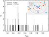 |
Fig. 5 Distribution of spectroscopic redshifts around the CC0958+0158 overdensity (see text). The gray and black histograms show the distribution within 600 and 2000 kpc, respectively. The inset shows the spatial distribution around the overdensity center of galaxies within Δz ~ 0.1 (or Δz ~ 0.2, smaller symbols) of the three spikes at z ~ 2.17, 2.19, 2.44, as indicated. The three gray circles have radii of 0.5, 1, 2 Mpc proper. |
Dedicated follow-up work is obviously still needed to verify whether these candidate overdensities are indeed signposts for early cluster environments. If successful, this approach would provide a further option for extending the investigation of distant cluster-like structures to the z ~ 2−2.5 range. In comparison with most other (proto-)cluster search techniques at these redshifts, e.g. the “IRAC selection” (e.g., Papovich et al. 2010; Stanford et al. 2012), targeted searches around radio galaxies (e.g., Venemans et al. 2007; Chiaberge et al. 2010; Wylezalek et al. 2013), 3D mapping (with spectroscopic or photometric redshifts, e.g., Diener et al. 2013; Scoville et al. 2013; Chiang et al. 2014; Mei et al. 2014), or overdensities of optically red galaxies (e.g., Andreon et al. 2009; Spitler et al. 2012), the approach discussed in this work is likely, by definition, to favor the most evolved environments, thus allowing a better probe of the diversity of cluster progenitors at a crucial time for the formation of both clusters and their massive galaxies.
An even better photo-z accuracy (as low as 1.5%, with a marked improvement at z ≳ 1.8) can be obtained by calibrating photo-zs on this sample with the more recent photometry from the Muzzin et al. (2013b) UltraVISTA catalog, in agreement with − and only marginally better than − photo-zs obtained by Muzzin et al. (2013b), as will be discussed in a forthcoming paper (Strazzullo et al., in prep.). Here we use the M10 catalog, which includes the southern part of the 2 sq. deg COSMOS field where one of our overdensities (Sect. 3.1) is found, which is not covered by the UltraVISTA survey (McCracken et al. 2012).
Acknowledgments
We thank M. Pannella and A. Saro for helpful input. V.S., E.D., R.G., and F.V. were supported by grants ERC-StG UPGAL 240039 and ANR-08-JCJC-0008. A.C. and M.M. acknowledge grants ASI n.I/023/12/0 and MIUR PRIN 2010-2011 “The dark Universe and the cosmic evolution of baryons; from current surveys to Euclid”. Based on observations from ESO Telescopes under program IDs 086.A-0681, 088.A-0671, LP175.A-0839, and 179.A-2005.
References
- Andreon, S., Maughan, B., Trinchieri, G., & Kurk, J. 2009, A&A, 507, 147 [NASA ADS] [CrossRef] [EDP Sciences] [Google Scholar]
- Andreon, S., Newman, A. B., Trinchieri, G., et al. 2014, A&A, 565, A120 [NASA ADS] [CrossRef] [EDP Sciences] [Google Scholar]
- Aravena, M., Carilli, C. L., Salvato, M., et al. 2012, MNRAS, 426, 258 [NASA ADS] [CrossRef] [Google Scholar]
- Bell, E. F., van der Wel, A., Papovich, C., et al. 2012, ApJ, 753, 167 [NASA ADS] [CrossRef] [Google Scholar]
- Belli, S., Newman, A. B., Ellis, R. S., & Konidaris, N. P. 2014, ApJ, 788, L29 [NASA ADS] [CrossRef] [Google Scholar]
- Bernardi, M., Nichol, R. C., Sheth, R. K., et al. 2006, AJ, 131, 1288 [NASA ADS] [CrossRef] [Google Scholar]
- Brammer, G. B., van Dokkum, P. G., & Coppi, P. 2008, ApJ, 686, 1503 [NASA ADS] [CrossRef] [Google Scholar]
- Brammer, G. B., van Dokkum, P. G., Franx, M., et al. 2012, ApJS, 200, 13 [Google Scholar]
- Brodwin, M., Stanford, S. A., Gonzalez, A. H., et al. 2013, ApJ, 779, 138 [NASA ADS] [CrossRef] [Google Scholar]
- Bruzual, G., & Charlot, S. 2003, MNRAS, 344, 1000 [NASA ADS] [CrossRef] [Google Scholar]
- Cappelluti, N., Brusa, M., Hasinger, G., et al. 2009, A&A, 497, 635 [NASA ADS] [CrossRef] [EDP Sciences] [Google Scholar]
- Cassata, P., Giavalisco, M., Williams, C. C., et al. 2013, ApJ, 775, 106 [NASA ADS] [CrossRef] [Google Scholar]
- Castignani, G., Chiaberge, M., Celotti, & Whatever, X. 2014, ApJ, 792, 114 [NASA ADS] [CrossRef] [Google Scholar]
- Chiaberge, M., Capetti, A., Macchetto, F. D., et al. 2010, ApJ, 710, L107 [NASA ADS] [CrossRef] [Google Scholar]
- Chiang, Y.-K., Overzier, R., & Gebhardt, K. 2014, ApJ, 782, L3 [NASA ADS] [CrossRef] [Google Scholar]
- Cimatti, A., Daddi, E., Renzini, A., et al. 2004, Nature, 430, 184 [NASA ADS] [CrossRef] [PubMed] [Google Scholar]
- Cimatti, A., Cassata, P., Pozzetti, L., et al. 2008, A&A, 482, 21 [NASA ADS] [CrossRef] [EDP Sciences] [Google Scholar]
- Daddi, E., Cimatti, A., Renzini, A., et al. 2004, ApJ, 617, 746 [NASA ADS] [CrossRef] [Google Scholar]
- Daddi, E., Renzini, A., Pirzkal, N., et al. 2005, ApJ, 626, 680 [NASA ADS] [CrossRef] [Google Scholar]
- De Lucia, G., Springel, V., White, S. D. M., et al. 2006, MNRAS, 366, 499 [NASA ADS] [CrossRef] [Google Scholar]
- Diener, C., Lilly, S. J., Knobel, C., et al. 2013, ApJ, 765, 109 [NASA ADS] [CrossRef] [Google Scholar]
- Diener, C., Lilly, S., Ledoux, C., et al. 2014, ApJ, submitted [arXiv:1411.0649] [Google Scholar]
- Elvis, M., Civano, F., Vignali, C., et al. 2009, ApJS, 184, 158 [NASA ADS] [CrossRef] [Google Scholar]
- Fassbender, R., Nastasi, A., Böhringer, H., et al. 2011, A&A, 527, L10 [NASA ADS] [CrossRef] [EDP Sciences] [Google Scholar]
- Finoguenov, A., Tanaka, M., Cooper, M., et al. 2015, A&A, in press DOI 10.1051/0004-6361/201323053 [Google Scholar]
- Gallazzi, A., Charlot, S., Brinchmann, J., et al. 2006, MNRAS, 370, 1106 [NASA ADS] [CrossRef] [Google Scholar]
- Gallazzi, A., Bell, E. F., Zibetti, S., et al. 2014, ApJ, 788, 72 [NASA ADS] [CrossRef] [Google Scholar]
- Gehrels, N. 1986, ApJ, 303, 336 [NASA ADS] [CrossRef] [Google Scholar]
- Gobat, R., Daddi, E., Onodera, M., et al. 2011, A&A, 526, A133 [NASA ADS] [CrossRef] [EDP Sciences] [Google Scholar]
- Gobat, R., Strazzullo, V., Daddi, E., et al. 2012, ApJ, 759, L44 [NASA ADS] [CrossRef] [Google Scholar]
- Gobat, R., Strazzullo, V., Daddi, E., et al. 2013, ApJ, 776, 9 [NASA ADS] [CrossRef] [Google Scholar]
- Hasinger, G., Cappelluti, N., Brunner, H., et al. 2007, ApJS, 172, 29 [NASA ADS] [CrossRef] [Google Scholar]
- Hayashi, M., Kodama, T., Koyama, Y., et al. 2010, MNRAS, 402, 1980 [NASA ADS] [CrossRef] [Google Scholar]
- Hilton, M., Lloyd-Davies, E., Stanford, S. A., et al. 2010, ApJ, 718, 133 [NASA ADS] [CrossRef] [Google Scholar]
- Ilbert, O., Capak, P., Salvato, M., et al. 2009, ApJ, 690, 1236 [NASA ADS] [CrossRef] [Google Scholar]
- Ilbert, O., McCracken, H. J., Le Fèvre, O., et al. 2013, A&A, 556, A55 [NASA ADS] [CrossRef] [EDP Sciences] [Google Scholar]
- Kauffmann, G., White, S. D. M., Heckman, T., et al. 2004, MNRAS, 353, 713 [NASA ADS] [CrossRef] [Google Scholar]
- Komatsu, E., Smith, K. M., Dunkley, J., et al. 2011, ApJS, 192, 18 [NASA ADS] [CrossRef] [Google Scholar]
- Kovač, K., Lilly, S. J., Knobel, C., et al. 2014, MNRAS, 438, 717 [NASA ADS] [CrossRef] [Google Scholar]
- Kriek, M., van Dokkum, P. G., Franx, M., et al. 2006, ApJ, 649, L71 [NASA ADS] [CrossRef] [Google Scholar]
- Kriek, M., van Dokkum, P. G., Labbé, I., et al. 2009, ApJ, 700, 221 [NASA ADS] [CrossRef] [Google Scholar]
- Krogager, J.-K., Zirm, A. W., Toft, S., & Whatever, X. 2014, ApJ, 797, 17 [NASA ADS] [CrossRef] [Google Scholar]
- Kurk, J., Cimatti, A., Zamorani, G., et al. 2009, A&A, 504, 331 [NASA ADS] [CrossRef] [EDP Sciences] [Google Scholar]
- Leauthaud, A., Finoguenov, A., Kneib, J.-P., et al. 2010, ApJ, 709, 97 [NASA ADS] [CrossRef] [Google Scholar]
- Lilly, S. J., Le Fèvre, O., Renzini, A., et al. 2007, ApJS, 172, 70 [NASA ADS] [CrossRef] [Google Scholar]
- Madau, P., & Dickinson, M. 2014, ARA&A, 52, 415 [NASA ADS] [CrossRef] [Google Scholar]
- Mancone, C. L., Gonzalez, A. H., Brodwin, M., et al. 2010, ApJ, 720, 284 [NASA ADS] [CrossRef] [Google Scholar]
- McCracken, H. J., Capak, P., Salvato, M., et al. 2010, ApJ, 708, 202 [NASA ADS] [CrossRef] [Google Scholar]
- McCracken, H. J., Milvang-Jensen, B., Dunlop, J., et al. 2012, A&A, 544, A156 [NASA ADS] [CrossRef] [EDP Sciences] [Google Scholar]
- Mei, S., Holden, B. P., Blakeslee, J. P., et al. 2009, ApJ, 690, 42 [NASA ADS] [CrossRef] [Google Scholar]
- Mei, S., Scarlata, C., Pentericci, L., et al. 2014, ApJ, submitted [arXiv:1403.7524] [Google Scholar]
- Muzzin, A., Wilson, G., Yee, H. K. C., et al. 2012, ApJ, 746, 188 [NASA ADS] [CrossRef] [Google Scholar]
- Muzzin, A., Marchesini, D., Stefanon, M., et al. 2013a, ApJ, 777, 18 [NASA ADS] [CrossRef] [Google Scholar]
- Muzzin, A., Marchesini, D., Stefanon, M., et al. 2013b, ApJS, 206, 8 [Google Scholar]
- Newman, A. B., Ellis, R. S., Andreon, S., et al. 2014, ApJ, 788, 51 [NASA ADS] [CrossRef] [Google Scholar]
- Onodera, M., Renzini, A., Carollo, M., et al. 2012, ApJ, 755, 26 [NASA ADS] [CrossRef] [Google Scholar]
- Papovich, C., Momcheva, I., Willmer, C. N. A., et al. 2010, ApJ, 716, 1503 [NASA ADS] [CrossRef] [Google Scholar]
- Planck Collaboration XVI. 2014, A&A, 571, A16 [NASA ADS] [CrossRef] [EDP Sciences] [Google Scholar]
- Salpeter, E. E. 1955, ApJ, 121, 161 [Google Scholar]
- Sánchez-Blázquez, P., Jablonka, P., Noll, S., et al. 2009, A&A, 499, 47 [NASA ADS] [CrossRef] [EDP Sciences] [Google Scholar]
- Santos, J. S., Fassbender, R., Nastasi, A., et al. 2011, A&A, 531, L15 [NASA ADS] [CrossRef] [EDP Sciences] [Google Scholar]
- Scoville, N., Arnouts, S., Aussel, H., et al. 2013, ApJS, 206, 3 [NASA ADS] [CrossRef] [Google Scholar]
- Spitler, L. R., Labbé, I., Glazebrook, K., et al. 2012, ApJ, 748, L21 [NASA ADS] [CrossRef] [Google Scholar]
- Stanford, S. A., Brodwin, M., Gonzalez, A. H., et al. 2012, ApJ, 753, 164 [NASA ADS] [CrossRef] [Google Scholar]
- Strazzullo, V., Rosati, P., Pannella, M., et al. 2010, A&A, 524, A17 [NASA ADS] [CrossRef] [EDP Sciences] [Google Scholar]
- Strazzullo, V., Gobat, R., Daddi, E., et al. 2013, ApJ, 772, 118 [NASA ADS] [CrossRef] [Google Scholar]
- Tanaka, M., Toft, S., Marchesini, D., et al. 2013, ApJ, 772, 113 [NASA ADS] [CrossRef] [Google Scholar]
- Toft, S., Gallazzi, A., Zirm, A., et al. 2012, ApJ, 754, 3 [NASA ADS] [CrossRef] [Google Scholar]
- Tran, K., Papovich, C., Saintonge, A., et al. 2010, ApJ, 719, L126 [CrossRef] [Google Scholar]
- Valentino, F., Daddi, E., Strazzullo, V., et al. 2014, ApJ, submitted [arXiv:1410.1437] [Google Scholar]
- Valentinuzzi, T., Poggianti, B. M., Fasano, G., et al. 2011, A&A, 536, A34 [NASA ADS] [CrossRef] [EDP Sciences] [Google Scholar]
- van de Sande, J., Kriek, M., Franx, M., et al. 2011, ApJ, 736, L9 [Google Scholar]
- van de Sande, J., Kriek, M., Franx, M., et al. 2013, ApJ, 771, 85 [NASA ADS] [CrossRef] [Google Scholar]
- van der Wel, A., Holden, B. P., Zirm, A. W., et al. 2008, ApJ, 688, 48 [NASA ADS] [CrossRef] [Google Scholar]
- Venemans, B. P., Röttgering, H. J. A., Miley, G. K., et al. 2007, A&A, 461, 823 [NASA ADS] [CrossRef] [EDP Sciences] [Google Scholar]
- Weiner, B. J. 2012 [arXiv:1209.1405] [Google Scholar]
- Williams, R. J., Quadri, R. F., Franx, M., et al. 2009, ApJ, 691, 1879 [NASA ADS] [CrossRef] [Google Scholar]
- Wuyts, S., Cox, T. J., Hayward, C. C., et al. 2010, ApJ, 722, 1666 [NASA ADS] [CrossRef] [Google Scholar]
- Wylezalek, D., Galametz, A., Stern, D., et al. 2013, ApJ, 769, 79 [NASA ADS] [CrossRef] [Google Scholar]
- Yuan, T., Nanayakkara, T., Kacprzak, G. G., et al. 2014, ApJ, 795, L20 [NASA ADS] [CrossRef] [Google Scholar]
All Figures
|
Fig. 1 Comparison of zphot vs. zspec for the full spectroscopic sample of 1.3 <z< 2.1 passive galaxies. Lower quality zspec determinations are shown in gray. Blue and red circles mark sources from the VIMOS and O12 samples, respectively. Orange stars highlight MIPS-detected sources. Dotted and solid lines show the bisector and a relative scatter of 2.5, 5, 10%. |
| In the text | |
|
Fig. 2 Distributions of K-band magnitude, stellar mass and photometric redshift for the sample of KAB< 23, z> 1.3 passive galaxies. Three leftmost panels: full sample (see text, black line), its pBzK subsample (red line), and the spectroscopic sample (scaled by × 10, red shaded area). Vertical dotted lines show the magnitude and mass (at z< 2.5) completeness limits of the parent K-selected catalog (see text). Rightmost panel: full photo-z distribution of the KAB< 23 passive sample (black line), and of its log(M/M⊙) > 10.9 subsample (shaded area, lighter gray at z> 2.5 where sample is beyond mass completeness). |
| In the text | |
|
Fig. 3 Examples of Σ5 maps in redshift slices of the full passive galaxy sample in the 2 sq. deg COSMOS field (North is up, East is left). Maps are scaled so that red colors correspond to > 5σ significance. The three candidate overdensities described in Sect. 3.1 are highlighted with white circles (2 Mpc radius proper). In each plot, the inset shows the distribution of log(Σ5) values in the map and its Gaussian fit (white and orange lines, respectively), and the white arrow shows the peak Σ5 value of the highlighted overdensity. |
| In the text | |
|
Fig. 4 Photo-z distributions for the whole (passive and star-forming) population of log(M/M⊙) > 10.9 galaxies within an aperture of r< 600 kpc from the three passive overdensities as labeled (red lines, errors as from Gehrels 1986). Galaxies and photo-zs used here are from Muzzin et al. (2013b) for CC1003+0223 and CC0958+0158, and from Ilbert et al. (2009) for CC1002+0134 (see text). In each panel, the blue line and dotted area show the median and 16th−84th percentiles of the photo-z distribution (from the same catalogs) in r< 600 kpc apertures at 100 random positions in the COSMOS field, while the grayed-out region shows the redshift range where the sample is no longer mass-complete. Black filled (empty) circles scattered above the histograms (at random y-axis coordinates) show our photo-z determinations for the passive sample used in this work within 300 kpc (600 kpc) from the overdensity center (larger/smaller symbols show galaxies more/less massive than log(M/M⊙) = 10.9). |
| In the text | |
|
Fig. 5 Distribution of spectroscopic redshifts around the CC0958+0158 overdensity (see text). The gray and black histograms show the distribution within 600 and 2000 kpc, respectively. The inset shows the spatial distribution around the overdensity center of galaxies within Δz ~ 0.1 (or Δz ~ 0.2, smaller symbols) of the three spikes at z ~ 2.17, 2.19, 2.44, as indicated. The three gray circles have radii of 0.5, 1, 2 Mpc proper. |
| In the text | |
Current usage metrics show cumulative count of Article Views (full-text article views including HTML views, PDF and ePub downloads, according to the available data) and Abstracts Views on Vision4Press platform.
Data correspond to usage on the plateform after 2015. The current usage metrics is available 48-96 hours after online publication and is updated daily on week days.
Initial download of the metrics may take a while.