| Issue |
A&A
Volume 575, March 2015
|
|
|---|---|---|
| Article Number | A75 | |
| Number of page(s) | 32 | |
| Section | Cosmology (including clusters of galaxies) | |
| DOI | https://doi.org/10.1051/0004-6361/201425419 | |
| Published online | 26 February 2015 | |
The MUSE 3D view of the Hubble Deep Field South⋆,⋆⋆
1
CRAL, Observatoire de Lyon, CNRS, Université Lyon 1,
9 avenue Ch. André,
69561
Saint Genis-Laval Cedex,
France
e-mail:
This email address is being protected from spambots. You need JavaScript enabled to view it.
2
Leiden Observatory, Leiden University,
PO Box 9513, 2300 RA
Leiden, The
Netherlands
3
IRAP, Institut de Recherche en Astrophysique et Planétologie,
CNRS, 14 avenue Édouard
Belin, 31400
Toulouse,
France
4
Université de Toulouse, UPS-OMP, 31400
Toulouse,
France
5
ETH Zurich, Institute of Astronomy, Wolfgang-Pauli-Str. 27, 8093
Zurich,
Switzerland
6
ESO, European Southern Observatory, Karl-Schwarzschild Str. 2, 85748
Garching bei Muenchen,
Germany
7
AIP, Leibniz-Institut für Astrophysik Potsdam,
An der Sternwarte 16,
14482
Potsdam,
Germany
8
AIG, Institut für Astrophysik, Universität
Göttingen, Friedrich-Hund-Platz
1, 37077
Göttingen,
Germany
9
Aix-Marseille Université, CNRS, LAM (Laboratoire d’Astrophysique
de Marseille) UMR 7326, 13388
Marseille,
France
Received: 27 November 2014
Accepted: 20 January 2015
Abstract
We observed Hubble Deep Field South with the new panoramic integral-field spectrograph MUSE that we built and have just commissioned at the VLT. The data cube resulting from 27 h of integration covers one arcmin2 field of view at an unprecedented depth with a 1σ emission-line surface brightness limit of 1 × 10-19 erg s-1 cm-2 arcsec-2, and contains ~90 000 spectra. We present the combined and calibrated data cube, and we performed a first-pass analysis of the sources detected in the Hubble Deep Field South imaging. We measured the redshifts of 189 sources up to a magnitude I814 = 29.5, increasing the number of known spectroscopic redshifts in this field by more than an order of magnitude. We also discovered 26 Lyα emitting galaxies that are not detected in the HST WFPC2 deep broad-band images. The intermediate spectral resolution of 2.3 Å allows us to separate resolved asymmetric Lyα emitters, [O ii]3727 emitters, and C iii]1908 emitters, and the broad instantaneous wavelength range of 4500 Å helps to identify single emission lines, such as [O iii]5007, Hβ, and Hα, over a very wide redshift range. We also show how the three-dimensional information of MUSE helps to resolve sources that are confused at ground-based image quality. Overall, secure identifications are provided for 83% of the 227 emission line sources detected in the MUSE data cube and for 32% of the 586 sources identified in the HST catalogue. The overall redshift distribution is fairly flat to z = 6.3, with a reduction between z = 1.5 to 2.9, in the well-known redshift desert. The field of view of MUSE also allowed us to detect 17 groups within the field. We checked that the number counts of [O ii]3727 and Lyα emitters are roughly consistent with predictions from the literature. Using two examples, we demonstrate that MUSE is able to provide exquisite spatially resolved spectroscopic information on the intermediate-redshift galaxies present in the field. Thisunique data set can be used for a wide range of follow-up studies. We release the data cube, the associated products, and the source catalogue with redshifts, spectra, and emission-line fluxes.
Key words: cosmology: observations / galaxies: evolution / galaxies: high-redshift / techniques: imaging spectroscopy / galaxies: formation
Advanced data products are available at http://muse-vlt.eu/science. Based on observations made with ESO telescopes at the La Silla Paranal Observatory under program ID 60.A-9100(C).
Appendices are available in electronic form at http://www.aanda.org
© ESO, 2015
1. Introduction
The Hubble Deep Fields North and South (see e.g. Williams et al., 1996; Ferguson et al., 2000; Beckwith et al., 2006) are still among the deepest images ever obtained in the optical/infrared, providing broad band photometry for sources up to V ~ 30. Coupled with extensive multi-wavelength follow-up campaigns they and the subsequent Hubble Ultra Deep Field have been instrumental in improving our understanding of galaxy formation and evolution in the distant Universe.
Deep, broad-band, photometric surveys provide a wealth of information on galaxy populations, such as galaxy morphology, stellar masses, and photometric redshifts. Taken together, this can be used to study the formation and evolution of the Hubble sequence (e.g. Mortlock et al., 2013; Lee et al., 2013), the change in galaxy sizes with time (e.g. van der Wel et al., 2014; Carollo et al., 2013), and the evolution of the stellar mass function with redshift (e.g. Muzzin et al., 2013; Ilbert et al., 2013). But photometric information alone gives only a limited view of the Universe: essential physical information, such as the kinematic state of the galaxies and their heavy element content, require spectroscopic observations. Furthermore, while photometric redshifts work well on average for many bright galaxies (e.g. Ilbert et al., 2009), they have insufficient precision for environmental studies and are occasionally completely wrong, and their performance on very faint galaxies is not well known.
Ideally, one would like to obtain spectroscopy for all sources at the same depth as the broad-band photometry. However current technology does not mach these requirements. For example, the VIMOS ultra-deep survey (Le Fevre et al., 2015), which is the largest spectroscopic deep survey today with 10 000 observed galaxies in 1 deg2, is in general limited to R ~ 25, and only 10% of the galaxies detected in the Hubble Deep Fields North and South are that bright.
Another fundamental limitation, when using multi-object spectrographs, is the need to pre-select a sample based on broad band imaging. Even if it was feasible to target all objects found in the Hubble deep fields WFPC2 deep images (i.e. ~6000 objects), the sample would still not include all galaxies with high equivalent-width emission lines, even though determining redshifts for these would be relatively easy. For example, faint low-mass galaxies with high star formation rate at high redshifts may not have an optical counterpart even in very deep HST broad-band imaging, although their emission lines arising in their star-forming interstellar medium might be detectable spectroscopically.
Long-slit observations are not a good alternative because of the limited field of view and other technical limitations due to slits such as unknown slit light losses, loss of positional information perpendicular to the slit and possible velocity errors. For example, Rauch et al. (2008) performed a long slit integration of 92 h with FORS2 at the VLT. They targeted the redshift range of 2.67−3.75, and their observations went very deep, with a emission-line surface-brightness limit (1σ) depth of 8.1 × 10⁻²⁰ erg s-1 cm-2 arcsec-2. However, this performance was obtained with a field of view of 0.25 arcmin2 and only one spatial dimension, limiting the usefulness of this technique for any follow-up surveys of Hubble deep fields.
To overcome some of these intrinsic limitations, a large, sensitive integral-field spectrograph is required. It must be sensitive and stable enough to be able to reach a depth commensurate to that of the Hubble deep fields, while at the same time having a high spatial resolution, large multiplex, spectral coverage, and good spectral resolution. This was at the origin of the Multi Unit Spectroscopic Explorer (MUSE) project to build a panoramic integral field spectrograph for the VLT (Bacon et al. 2010; and in prep.). The commissioning of MUSE on the VLT was completed in August 2014 after development by a consortium of seven European institutes: CRAL (lead), AIG, AIP, ETH-Zurich, IRAP, NOVA/Leiden Observatory and ESO. The instrument has a field of view of 1 × 1 arcmin2 sampled at 0.2 arcsec, an excellent image quality (limited by the 0.2 arcsec sampling), a wide simultaneous spectral range (4650−9300 Å), a medium spectral resolution (R ≃ 3000), and a very high throughput (35% end-to-end including telescope at 7000 Å).
Although MUSE is a general purpose instrument and has a wide range of applications (see Bacon et al. 2014, for a few illustrations), it has been, from the very start of the project in 2001, designed and optimised for performing deep field observations. Some preliminary measurements during the first commissioning runs had convinced us that MUSE was able to reach its combination of high throughput and excellent image quality. However it is only by performing a very long integration on a deep field that one can assess the ultimate performance of the instrument. This was therefore one key goal of the final commissioning run of ten nights in dark time late July 2014. The Hubble Deep Field South (HDFS) which was observable during the second half of the nights for a few hours, although at relatively high airmass, was selected as the ideal target to validate the performance of MUSE, the observing strategy required for deep fields to limit systematic uncertainties and to test the data reduction software.
The HDFS was observed with the Hubble Space Telescope in 1998 (Williams et al., 2000). The WFPC2 observations (Casertano et al., 2000) reach a 10σ limiting AB magnitude in the F606W filter (hereafter V606) at 28.3 and 27.7 in the F814W filter (hereafter I814). The field was one of the first to obtain very deep Near-IR multi-wavelength observations (e.g., Labbé et al. 2003). But, contrarily to the Hubble Ultra Deep Field (Beckwith et al., 2006) which had very extensive spectroscopic follow-up observations, the main follow-up efforts on the HDFS have been imaging surveys (e.g. Labbé et al. 2003, 2005).
In the present paper we show that the use of a wide-field, highly sensitive IFU provides a very powerful technique to target such deep HST fields, allowing a measurement of ~200 redshifts per arcmin2, ~30 of which are not detected in the HDF continuum images. We present the first deep observations taken with the MUSE spectrograph, and we determine a first list of secure redshifts based on emission-line and absorption-line features. We show that the high spectral resolution, broad wavelength range, and three dimensional nature of the data help to disentangle confused galaxies and to identify emission lines securely.
The paper is organised as follows: the observations, data reduction and a first assessment of instrument performance are described in the next two sections. In Sects. 4 and 5, we proceed with the source identifications and perform a first census of the field content. The resulting redshift distribution and global properties of the detected objects are presented in Sect. 6. Examples of kinematics analysis performed on two spatially resolved galaxies is given in Sect. 7. Comparison with the current generation of deep spectroscopic surveys and conclusions are given in the last section. The data release is described in the Appendices.
2. Observations
The HDFS was observed during six nights in July 25−29, 31 and August 2, 3 2014 of the last commissioning run of MUSE. The 1 × 1 arcmin2 MUSE field was centred at α = 22h32′55.64′′, δ = −60°33′47′′. This location was selected in order to have one bright star in the Slow Guiding System (SGS) area and another bright star in the field of view (Fig. 1). We used the nominal wavelength range (4750−9300 Å) and performed a series of exposures of 30 min each. The spectrograph was rotated by 90° after each integration, and the observations were dithered using random offsets within a 3 arcsec box. This scheme ensures that most objects will move from one channel1 to a completely different one while at the same time minimizing the field loss. This is, however, not true for the objects that fall near the rotation centre.
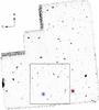 |
Fig. 1 Location of the MUSE field of view within the HDFS F814W image. The star used in the slow guiding system is indicated in red and the brightest star in the field (R = 19.6) in blue. |
In addition to the standard set of calibrations, we obtained a flat field each hour during the night. These single flat field exposures, referred to as attached flats in the following, are used to correct for the small illumination variations caused by temperature variations during the night. The Slow Guiding System was activated for all exposures using a bright R = 19.2 star located in the SGS field. The SGS also gives an accurate real-time estimate of the seeing which was good for most of the nights (0.5−0.9 arcsec). Note that the values given by the SGS are much closer to the seeing achieved in the science exposure than the values given by the DIMM seeing monitor. An astrometric solution was derived using an off-centre field of a globular cluster with HST data. A set of spectrophotometric standard stars was also observed when the conditions were photometric.
In total, 60 exposures of 30 min integration time were obtained. A few exposures were obtained in cloudy conditions and were discarded. One exposure was lost due to an unexpected VLT guide star change in the middle of the exposure. The remaining number of exposures was 54, with a total integration time of 27 h. One of these exposures was offset by approximately half the field of view to test the performance of the SGS guiding on a faint galaxy.
3. Data reduction and performance analysis
3.1. Data reduction process
The data were reduced with version 0.90 of the MUSE standard pipeline. The pipeline will be described in detail in Weilbacher et al. (in prep.)2. We summarize the main steps to produce the fully reduced data cube:
-
1.
Bias, arcs and flat-field master calibration solutions were created using a set of standard calibration exposures obtained each night.
-
2.
Bias images were subtracted from each science frame. Given its low value, the dark current (~ 1 e− h-1, that is 0.5 e− per exposure) was neglected. Next, the science frames were flat-fielded using the master flat field and renormalized using the attached flat field as an illumination correction. An additional flat-field correction was performed using the twilight sky exposures to correct for the difference between sky and calibration unit illumination. The result of this process is a large table (hereafter called a pixel-table) for each science frame. This table contains all pixel values corrected for bias and flat-field and their location on the detector. A geometrical calibration and the wavelength calibration solution were used to transform the detector coordinate positions to wavelengths in Ångström and focal plane spatial coordinates.
-
3.
The astrometric solution was then applied. The flux calibration was obtained from observations of the spectrophotometric standard star Feige 110 obtained on August 3, 2014. We verified that the system response curve was stable between the photometric nights with a measured scatter below 0.2% rms. The response curve was smoothed with spline functions to remove high frequency fluctuations left by the reduction. Bright sky lines were used to make small corrections to the wavelength solution obtained from the master arc. All these operations have been done at the pixel-table level to avoid unnecessary interpolation. The formal noise was also calculated at each step.
-
4.
To correct for the small shifts introduced by the derotator wobble between exposures, we fitted a Gaussian function to the brightest star in the reconstructed white-light image of the field. The astrometric solution of the pixel-tables of all exposures was normalized to the HST catalogue coordinate of the star (α = 22h37′57.0′′, δ = −60°34′06′′) The fit to the star also provides an accurate measurement of the seeing of each exposure. The average Gaussian white-light full width at half maximum (FWHM) value for the 54 exposures is 0.77 ± 0.15 arcsec. We also derived the total flux of the reference star by simple aperture photometry, the maximum variation among all retained exposures is 2.4%.
-
5.
To reduce systematic mean zero-flux level offsets between slices, we implemented a non-standard self-calibration process. From a first reconstructed white-light image produced by the merging of all exposures, we derived a mask to mask out all bright continuum objects present in the field of view. For each exposure, we first computed the median flux over all wavelengths and the non-masked spatial coordinates. Next we calculated the median value for all slices, and we applied an additive correction to each slice to bring all slices to the same median value. This process very effectively removed residual offsets between slices.
-
6.
A data cube was produced from each pixel-table using a 3D drizzle interpolation process which include sigma-clipping to reject outliers such as cosmic rays. All data cubes were sampled to a common grid in view of the final combination (
 Å).
Å). -
7.
We used the software ZAP (Soto et al., in prep.) to subtract the sky signal from each of the individual exposures. ZAP operates by first subtracting a baseline sky level, found by calculating the median per spectral plane, leaving any residuals due to variations in the line spread function (LSF) and system response. The code then uses principal component analysis on the data cube to calculate the eigenspectra and eigenvalues that characterize these residuals, and determines the minimal number of eigenspectra that can reconstruct the residual emission features in the data cube.
-
8.
The 54 data cubes were then merged in a single data cube using 5σ sigma-clipped mean. The variance for each combined volume pixel or “voxel” was computed as the variance derived from the comparison of the N individual exposures divided by N − 1, where N is the number of voxels left after the sigma-clipping. This variance data cube is saved as an additional extension of the combined data cube. In addition an exposure map data cube which counts the number of exposures used for the combination of each voxel was also saved.
-
9.
Telluric absorption from H2O and O2 molecules was fitted to the spectrum of a white dwarf found in the field (α = 22h32′58.77′′, δ = −60°33′23.52′′) using the molecfit software described in Smette et al. (2015) and Kausch et al. (2015). In the fitting process, the LSF was adjusted using a wavelength dependent Gaussian kernel. The resulting transmission correction was then globally applied to the final data cube and variance estimation.
The result of this process is a fully calibrated data cube of 3 Gb size with spectra in the first extension and the variance estimate in the second extension, as well as an exposure cube of 1.5 Gb size giving the number of exposures used for each voxel.
3.2. Reconstructed white-light image and point-spread functions
The image quality was assessed using a Moffat fit of the reference star as a function of wavelength. The PSF shape is circular with a fitted Moffat β parameter of 2.6 and a FWHM of 0.66 arcsec at 7000 Å. While β is almost constant with wavelength, the FWHM shows the expected trend with wavelength decreasing from 0.76 arcsec in the blue to 0.61 arcsec in the red (Fig. 2). Note that the FWHM derived from the MOFFAT model is systematically 20% lower than the Gaussian approximation.
The spectral LSF was measured on arc calibration frames. We obtain an average value of 2.1 ± 0.2 pixels which translates into a spectral resolution of R3000 ± 100 at 7000 Å. A precise measurement of the LSF shape is difficult because it is partially under sampled. In the present case this uncertainty is not problematic because the spectral features of the identified objects are generally broader than the LSF.
A simple average over all wavelengths gave the reconstructed white light image (Fig. 3). Inspection of this image reveals numerous objects, mostly galaxies. The astrometric accuracy, derived by comparison with the Casertano et al. (2000) catalogue, is ~0.1 arcsec. At lower flux levels, F ~ 2 × 10-21 erg s-1 cm-2 Å-1 pixel-1, some residuals of the instrument channel splitting can be seen in the reconstructed white-light image in the form of a series of vertical and horizontal stripes.
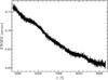 |
Fig. 2 Derived FWHM as function of wavelength from the Moffat fit to the brightest star in the field. |
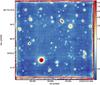 |
Fig. 3 Reconstructed white-light image of the combined exposures. The flux scale shown on the right is in 10-21 erg s-1 cm-2 Å-1 pixel-1. Orientation is north(up)-east(left). |
3.3. Signal to noise ratios
Characterising the noise in a MUSE data cube is not trivial, as each voxel of the cube is interpolated not only spatially, but also in the spectral domain, and each may inherit flux from just one up to ~30 original CCD pixels. While readout and photon noise are formally propagated by the MUSE pipeline as pixel variances, correlations between two neighbouring spatial pixels cause these predicted variances to be systematically too low. Furthermore, the degree of correlation between two neighbouring spatial pixels varies substantially across the field (and with wavelength), on spatial scales comparable to or larger than real astronomical objects in a deep field such as the HDFS. A correct error propagation also accounting for the covariances between pixels is theoretically possible, but given the size of a MUSE dataset this is unfortunately prohibitive with current computing resources. We therefore have to find other ways to estimate the “true” noise in the data.
For the purpose of this paper we focus on faint and relatively small sources, and we therefore neglect the contribution of individual objects to the photon noise. In addition to readout and sky photon noise, unresolved low-level systematics can produce noise-like modulations of the data, especially when varying rapidly with position and wavelength. Such effects are certainly still present in MUSE data, e.g. due to the residual channel and slice splitting pattern already mentioned in Sect. 3. Another issue are sky subtraction residuals of bright night sky emission lines which are highly nonuniform across the MUSE field of view. Future versions of the data reduction pipeline will improve on these features, but for the moment we simply absorb them into an “effective noise” budget.
In the HST image of the HDFS we selected visually a set of 100 “blank sky” locations free from any continuum or known emission line sources. These locations were distributed widely over the MUSE field of view, avoiding the outskirts of the brightest stars and galaxies. We extracted spectra through circular apertures from the sky-subtracted cube which consequently should have an expectation value of zero at all wavelengths. Estimates of the effective noise were obtained in two different ways: (A) By measuring the standard deviation inside of spectral windows selected such that no significant sky lines are contained; (B) by measuring the standard deviation of aperture-integrated fluxes between the 100 locations, as a function of wavelengths. Method (A) directly reproduces the “noisiness” of extracted faint-source spectra, but cannot provide an estimate of the noise for all wavelengths. Method (B) captures the residual systematics also of sky emission line subtraction, but may somewhat overestimate the “noisiness” of actual spectra. We nevertheless used the latter method as a conservative approach to construct new “effective” pixel variances that are spatially constant and vary only in wavelength. Overall, the effective noise is higher by a factor of ~1.4 than the local pixel-to-pixel standard deviations, and by a factor of ~1.6 higher than the average propagated readout and photon noise. Close to the wavelengths of night sky emission lines, these factors may get considerably higher, mainly because of the increased residuals.
The median effective noise per spatial and spectral pixel for the HDFS data cube is then 9 × 10-21 erg s-1 cm-2 Å-1, outside of sky lines. For an emission line extending over 5 Å (i.e. 4 spectral pixels), we derive a 1σ emission line surface brightness limit of 1 × 10-19 erg s-1 cm-2 arcsec-2.
An interesting comparison can be made with the Rauch et al. (2008) deep long slit integration. In 92 h, they reached a 1σ depth of 8.1 × 10⁻²⁰ erg s-1 cm-2 arcsec-2, again summed over 5 Å. Rauch et al. covered the wavelength range 4457−5776 Å, which is 3.4× times smaller than the MUSE wavelength range, and they cover an area (0.25 arcmin2) which is four times smaller. Folding in the ratio of exposure times and the differences in achieved flux limits, the MUSE HDFS data cube is then in total over 32 times more effective for a blind search of emission line galaxies than the FORS2 observation. This is not a surprise given that FORS2 was not designed for this specific application but for imaging and slit spectroscopy over a ~20 arcmin2 field of view.
From the limiting flux surface brightness one can also derive the limiting flux for a point source. This is, however, more complex because it depends of the seeing and the extraction method. A simple approximation is to use fix aperture. For a 1 arcsec diameter aperture, we measured a light loss of 40% at 7000 Å for the brightest star in the MUSE field. Using this value, we derive an emission line limiting flux at 5σ of 3 × 10-19 erg s-1 cm-2 for a point source within a 1 arcsec aperture.
For a better understanding of the contribution of systematics to the noise budget, we also investigated the scaling of the noise with exposure time. Taking the effective noise in a single 30 min exposure as unit reference, we also measured the noise in coadded cubes of 4, 12, and the full set of 54 exposures. While systematic residuals are also expected to decrease because of the rotational and spatial dithering, they would probably not scale with  as perfect random noise. The result of this exercise is shown in Fig. 4, which demonstrates that a significant deviation from is detected, but that it is quite moderate (factor ~1.2 for the full HDFS cube with n = 54). Even without reducing the systematics, adding more exposures would make the existing HDFS dataset even deeper.
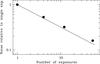 |
Fig. 4 Overall scaling of pixel noise measured in the cubes as a function of the number of exposures combined, relative to the noise in a single exposure. The solid line represents the ideal |
4. Source identification and redshift determination
The three-dimensional nature of the MUSE observations presents unique challenges, while at the same time offering multiple ways to extract spectra and to determine and confirm redshifts. We have found that constructing 1D and 2D projections of the sources is essential to ascertain redshifts for the fainter sources. In particular we have constructed 1D spectra and for each tentative emission line we construct a continuum subtracted narrow-band image over this line, typically with a width of 10 Å, and only if this produces a coherent image of the source we consider the emission line real. Likewise, 2D spectra can be useful additional tools for understanding the spatial distribution of emission.
The extraction of spectra from a very deep data cube can be challenging since the ground based seeing acts to blend sources. Here too the construction of 2D images can help disentangling sources that otherwise would be blended. For this step the existence of deep HST images is very helpful to interpret the results.
This method does not lend itself to absorption line redshifts. In this case we examine the spatial variation of possible absorption line features by extracting spectra at various spatial positions. A real absorption line should be seen in multiple spectra across the galaxy.
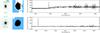 |
Fig. 5 Example of the extraction process for objects 5 and 144, at z = 0.58 and z = 4.02 respectively. Top row the left panel: MUSE reconstructed white-light image, while the left panel in the bottom row shows the Lyα narrow-band image. Middle panels: object and sky masks, with the object aperture shown in black and the sky aperture in blue. Part of the final extracted spectrum is shown in the right-hand panel on each row. |
4.1. Redshift determination of continuum detected objects
We extracted subcubes around each object in the Casertano et al. (2000) catalogue that fell within the FoV sampled by the observations. We defined our spectrum extraction aperture by running SExtractor (Bertin & Arnouts, 1996), version 2.19.5 on the reconstructed white-light images. In the case when no object was clearly detected in the white-light image, a simple circular extraction aperture with diameter 1.4′′ was used. When a redshift was determined, we constructed narrow-band images around Ly-α, C iii]1909, [O ii]3727, Hβ, [O iii]5007, and Hα, whenever that line fell within the wavelength range of MUSE, and ran SExtractor on these as well. The union of the emission-line and the white-light segmentation maps define our object mask. The SExtractor segmentation map was also used to provide a sky mask. The object and sky masks were inspected and manually adjusted when necessary to mask out nearby sources and to avoid edges.
The local sky residual spectrum is constructed by averaging the spectra within the sky mask. The object spectrum was constructed by summing the spectra within the object mask, subtracting off the average sky spectrum in each spatial pixel (spaxel). We postpone the optimal extraction of spectra (e.g. Horne, 1986) to future work as this is not essential for the present paper. Note also that we do not account for the wavelength variation of the PSF in our extraction – this is a significant concern for optimal extraction but for the straight summation we found by testing on stars within the data cube that the effect is minor for extraction apertures as large as ours.
An example of the process can be seen in Fig. 5. The top row shows the process for a z ≈ 0.58 galaxy with the white-light image shown in the left-most column, and the bottom row the same for a Lyα-emitter at z = 4.02 with the Lyα-narrow-band image shown in the left-most column. The region used for the local sky subtraction is shown in blue in the middle column, while the object mask is shown in black.
The resulting spectra were inspected manually and emission lines and absorption features were identified by comparison to template spectra when necessary. In general an emission line redshift was considered acceptable if a feature consistent with an emission line was seen in the 1D spectrum and coherent spatial feature was seen in several wavelength planes over this emission line. In some cases mild smoothing of the spectrum and/or the cube was used to verify the reality of the emission line. In the case of absorption line spectra several absorption features were required to determine a redshift.
In many cases this process gives highly secure redshifts, with multiple lines detected in 72 galaxies and 8 stars. We assign them a Confidence = 3. In general the identification of single line redshifts is considerably less challenging than in surveys carried out with low spectral resolution. The [O ii]3726, 3729 and C iii]1907, 1909 doublets are in most cases easily resolved and the characteristic asymmetric shape of Lyα is easily identified. In these cases we assign a Confidence = 2 for single-line redshifts with high signal-to-noise (S/N). In a number of cases we do see unresolved [O ii]3726, 3729 – in these cases we still have a secure redshift from Balmer absorption lines and/or [Ne iii]3869 – but these lines are unresolved due to velocity broadening and we do not expect to see this behaviour in spectra of very faint galaxies. The other likely cases of single line redshifts with a symmetric line profile are: Hα-emitters with undetected [N ii]6584 and no accompanying strong [O iii]5007; [O iii]5007 emitters with undetectable [O iii]4959 and Hβ; and Lyα-emitters with symmetric line profiles.
To distinguish between these alternatives, we make use of two methods. The first is to examine the continuum shape of the spectra. For the brighter objects breaks in the spectra can be used to separate between the various redshift solutions. The second method is to check the spectrum at the location of any other possible line, and to extract narrow-band images for all possible strong lines – this is very useful for [O iii]5007 and Hα emitters, and can exclude or confirm low redshift solutions. If this process does not lead to a secure redshift, we assign a confidence 0 to these sources. The redshift confidence assignments is summarized below:
-
0: No secure or unique redshift determination possible;
-
1: Redshift likely to be correct but generally based on only one feature;
-
2: Redshift secure, but based on one feature;
-
3: Redshift secure, based on several features.
In the case of overlapping sources we do not attempt to optimally extract the spectrum of each source, leaving this to future papers. In at least four cases we see two sets of emission lines in the extracted spectrum and we are unable to extract each spectrum separately. Despite this we are still generally able to associate a redshift to a particular object in the HST catalogue by looking at the distribution of light in narrow-band images. We also use these narrow band images to identify cases where a strong emission line in a nearby object contaminates the spectrum of a galaxy.
4.2. Identification of line emitters without continuum
In parallel to the extraction of continuum-selected objects, we also searched for sources detected only by their line emission. Two approaches were used: a visual inspection of the MUSE data cube, and a systematic search using automatic detection tools.
Two of the authors (JR, TC) visually explored the data cube over its full wavelength range in search of sources appearing only in a narrow wavelength range, typically 4−5 wavelength planes (~6−7 Å), and seemingly extended over a number of pixels at least the size of the seeing disk. We then carefully inspected the extracted line profile around this region to assess the reality of the line.
Any visual inspection has obvious limits and we also employed more automatic tools for identifying sources dominated by emission lines. One such tool is based on SExtractor (Bertin & Arnouts, 1996) which was run on narrow-band images produced by averaging each wavelength plane of the cube with the 4 closest wavelength planes, adopting a weighting scheme which follows the profile on an emission line with a velocity σ = 100 km s-1. This procedure was performed accross the full wavelength range of the cube to enhance the detection of single emission lines (see also Richard et al. 2015). All SExtractor catalogues obtained from each narrow-band image were merged and compared with the continuum estimation from the white light image to select emission lines.
A different approach was used in the LSDCat software (Herenz, in prep.), which was specifically designed to search for line emitters not associated with continuum sources in the MUSE data cube. The algorithm is based on matched filtering (e.g. Das 1991): by cross-correlating the data cube with a template that resembles the expected 3D-signal of an emission line, the S/N of a faint emission line is maximized. The optimal template for the search of compact emission line objects is a function that resembles the seeing PSF in the spatial domain and a general emission line shape in the spectral domain. In practice we use a 3D template that is a combination of a 2D Moffat profile with a 1D Gaussian spectral line. The 2D Moffat parameters is taken from the bright star fit (see Fig. 2 in Sect. 3) and the FWHM of the Gaussian is fixed to 300 km s-1 in velocity space. To remove continuum signal, we median-filter the data cube in the spectral direction and subtract this cube from the original cube. In the following cross-correlation operation the variances are propagated accordingly, and the final result is a data cube that contains a formal detection significance for the template in each cube element (voxel). Thresholding is performed on this data cube, where regions with neighbouring voxels above the detection threshold are counted as one object and a catalogue of positions (x,y,λ) of those detections is created. To limit the number of false detections due to unaccounted systematics from sky-subtraction residuals in the redder part of the data cube, a detection threshold of 10σ was used. The candidate sources were then visually inspected by 3 authors (CH, JK & JB). This process results in the addition of 6 new identifications that had escaped the previous inspections.
All the catalogues of MUSE line emitters described above were cross-correlated with the Casertano et al. (2000) catalogue of continuum sources presented in Sect. 4.1. A few of the emission lines were associated with continuum sources based on their projected distance in the plane of the sky. Isolated emission lines not associated with HST continuum sources were treated as separate entries in the final catalogue and their spectra were extracted blindly at the locations of the line emission. The spectral extraction procedure was identical to the one described in Sect. 4.1.
The very large majority of line emitters not associated with HST continuum detections show a clear isolated line with an asymmetric profile, which we associate with Lyα emission. In most case this is corroborated by the absence of other strong lines (except possibly C iii] emission at 2.9 <z< 4) and the absence of a resolved doublet (which would be expected in case of [O ii] emission).
4.3. Line flux measurements
We measure emission line fluxes in the spectra using the platefit code described by Tremonti et al. (2004) and Brinchmann et al. (2004) and used for the MPA-JHU catalogue of galaxy parameters from the SDSS3. This fits the stellar spectrum using a non-negative least-squares combination of theoretical spectra broadened to match the convolution of the velocity dispersion and the instrumental resolution. It then fits Gaussian profiles to emission lines in the residual spectrum. Because of its asymmetric shape, this is clearly not optimal for Lyα and we describe a more rigorous line flux measurement for this line in Sect. 6.3 below.
The S/N in most spectra is insufficient for a good determination of the stellar velocity dispersion, so for the majority of galaxies we have assumed a fixed intrinsic velocity dispersion of 80 km s-1. This resulted in good fits to the continuum spectrum for most galaxies and changing this to 250 km s-1 changes forbidden line fluxes by less than 2%, while for Balmer lines the effect is <5% for those galaxies for which we cannot measure a velocity dispersion. These changes are always smaller than the formal flux uncertainty and we do not consider these further here.
The emission lines are fit jointly with a single width in velocity space and a single velocity offset relative to the continuum redshift. Both the [O ii]3726, 3729 and C iii]1906, 1908 doublets are fit separately so the line ratios can be used to determine electron density. We postpone this calculation for future work.
4.4. Comparison between MUSE and published spectroscopic redshifts
Several studies have provided spectroscopic redshifts for sources in the HDFS and its flanking fields:
-
Sawicki & Mallén-Ornelas (2003) presented spectroscopic redshifts for 97 z< 1 galaxies with FORS2 at the VLT. Their initial galaxy sample was selected based on photometric redshifts, zphot ≲ 0.9 and their resulting catalogue is biased towards z ~ 0.5 galaxies. The spectral resolution (R ~ 2500−3500) was sufficient to resolve the [O ii]3727 doublet, enabling a secure spectroscopic redshift determination. The typical accuracy that they quote for their spectroscopic redshifts is δz = 0.0003.
-
Rigopoulou et al. (2005) followed up 100 galaxies with FORS1 on the VLT, and measured accurate redshifts for 50 objects. Redshifts were determined based on emission lines (usually [O ii]3727) or, in a few cases, absorption features such as the CaII H, K lines. The redshift range of the spectroscopically-detected sample is 0.6−1.2, with a median redshift of 1.13. These redshifts agree well with the Sawicki & Mallén-Ornelas (2003) estimates for sources in common between the two samples.
-
Iwata et al. (2005) presented VLT/FORS2 spectroscopic observations of galaxies at z ~ 3; these were selected to have 2.5 <zphot < 4 based on HST/WFPC2 photometry combined with deep near-infrared images obtained with ISAAC at the VLT by Labbé et al. (2003). They firmly identified five new redshifts as well as two additional tentative redshifts of z ~ 3 galaxies.
-
Glazebrook et al. (2006) produced 53 additional extragalactic redshifts in the range 0 <z< 1.4 with the AAT Low Dispersion Survey Spectrograph by targeting 200 objects with R > 23.
-
Finally Wuyts et al. (2009) used a variety of optical spectrographs on 8−10 m class telescopes (LRIS and DEIMOS at Keck Telescope, FORS2 at the VLT and GMOS at Gemini South) to measure redshifts for 64 optically faint distant red galaxies.
In total these long term efforts have provided a few hundred spectroscopic redshifts. They are, however, distributed over a much larger area than the proper HDFS deep imaging WFPC2 field, which has only ~88 confirmed spectroscopic redshifts. In the MUSE field itself, which covers 20% of the WFPC2 area, we found 18 sources in common (see Table A.3). As shown in Fig. 16, most of the 18 sources cover the bright part (I814 < 24) of the MUSE redshift-magnitude distribution.
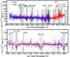 |
Fig. 6 Comparison between the MUSE (red) and FORS1 spectra of Rigopoulou et al. (2005; blue) for the galaxy ID#13, a strong [O ii] emitter at zMUSE = 1.2902. The strongest spectral features are indicated in black. The grey lines show the position of the sky lines. Upper panel: entire spectra; lower panel: zoom on the rest-frame 2300−2800 Å region, which contains strong MgII and FeII absorption features. |
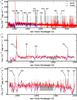 |
Fig. 7 Comparison between the MUSE (red) and FORS2 spectra of Iwata et al. (2005; blue) for the galaxy ID#43, a strong Lyα emitter at zMUSE = 3.2925. The strongest spectral features are indicated in black. The grey lines show the position of the sky lines; grey areas show wavelength regions for which no FORS2 spectrum was published. Upper panel: entire spectra; middle and lower panels: zoom on the Lyα and 1380−1550 Å region, respectively; the latter contains strong SiIV absorption features. |
Generally speaking there is an excellent agreement between the different redshift estimates over the entire redshift range covered by the 18 sources. Only one major discrepancy is detected: ID#2 (HDFS J223258.30-603351.7), which Glazebrook et al. (2006) estimated to be at redshift 0.7063 while MUSE reveals it to be a star. These authors gave however a low confidence grade of ~50% to their identification. After excluding this object, the agreement is indeed excellent with a normalized median difference of ⟨Δz/ (1 + z)⟩ = 0.00007 between MUSE and the literature estimates.
For two of the galaxies in common with other studies, ID#13 (HDFS J223252.16-603323.9) and ID#43 (HDFS J223252.03-603342.6), the actual spectra have been published together with the estimated redshifts. This enables us to perform a detailed comparison between these published spectra and our MUSE spectra (integrated over the entire galaxy). This comparison is shown in Figs. 6 and 7 for ID#13 (Rigopoulou et al., 2005) and ID#43 (Iwata et al., 2005), respectively.
The galaxy ID#13 is a strong [O ii]3727 emitter at zMUSE = 1.2902. In the top panel of Fig. 6 its full FORS1 and MUSE spectra are shown in blue and red, respectively. The FORS1 spectrum covers only the rest-frame λ< 3500 Å wavelength region, which does not include the [O ii] feature. The lower panel of the figure shows a zoom on the rest-frame ~2300−2800 Å window, which includes several strong Fe and Mg absorption features. The MUSE spectrum resolves the FeII and MgII doublets well; it is also clear that some strong features in the FORS1 spectrum, e.g., at ~2465 Å, 2510 Å, 2750 Å and 2780 Å are not seen in the high S/N MUSE spectrum.
The galaxy ID#43 is a Lyα emitter at zMUSE = 3.2925. Figure 7 shows the MUSE spectrum in red and the FORS2 spectrum of Iwata et al. (2005) in blue. The middle and bottom panels show zooms on the Lyα emission line and the rest-frame ~1380−1550 Å Si absorption features, respectively. The higher S/N and resolution of the MUSE spectrum opens the way to quantitative astrophysical studies of this galaxy, and generally of the early phases of galaxy evolution that precede the z ~ 2 peak in the cosmic star-formation history of the Universe.
4.5. Comparison between MUSE and published photometric redshifts
Our analysis of the HDFS allows for a quantitative comparison with photometric redshifts from the literature. We make a first comparison to the photometric redshift catalogue of Labbé et al. (2003) who used the FIRES survey to complement existing HST imaging with J, H, and Ks band data reaching  . We find 89 objects in common between the two catalogues, including 8 stars. The comparison is given in Fig. 8. Considering the 81 non-stellar objects, we quantify the agreement between the MUSE spectroscopic redshifts and the 7-band photometric redshifts of Labbé et al. (2003) by calculating σNMAD (Eq. (1)of Brammer et al. 2008). This gives the median absolute deviation of Δz, and quantifies the number of “catastrophic outliers”, defined as those objects with | Δz | > 5σNMAD.
 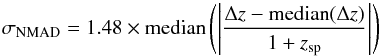 (1)where Δz = (zsp − zph).
We find σNMAD = 0.072 with 6 catastrophic outliers, equating to 7.4 percent of the sample. Excluding outliers and recomputing results in σNMAD = 0.064 reduces the number of catastrophic outliers to 2 objects, 2.7 percent of the remaining 75 sources.
Of the 6 outlying objects, 5 are robustly identified as [O ii] emitters in our catalogue, but the photometric redshifts put all 5 of these objects at very low redshift, most likely due to template mismatch in the SED fitting. The final object’s spectroscopic redshift is z = 0.83, identified through absorption features, but the photometric redshift places this object at z = 4.82. This is not a concern, as the object exhibits a large asymmetric error on the photometric redshift bringing it into agreement with zsp. As noted in Labbé et al. (2003), this often indicates a secondary solution to the SED-fitting with comparable probability to the primary solution, at a very different redshift.
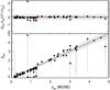 |
Fig. 8 Comparison of MUSE spectroscopic redshifts with the photometric redshifts of Labbé et al. (2003). Upper panel: distribution of Δz as a function of MUSE zsp with outliers highlighted in red. The error bars shows the uncertainties reported by Labbé et al. The grey shaded area depicts the region outside of which objects are considered outliers. Lower panel: direct comparison of MUSE zsp and Labbé et al. (2003)zph with outliers again highlighted in red. |
The advantage of a blind spectroscopic survey such as ours is highlighted when considering the reliability of photometric redshifts for the faint emission-line objects we detect in abundance here. Figure 9 shows values of Δz/ (1 + z) for objects in our catalogue with an HST detection in the F814W filter. For galaxies with magnitude below I814 = 24, the measured scatter (rms) 3.7%, is comparable to what is usually measured (e.g. Saracco et al. 2006; Chen et al. 1998). However, at fainter magnitudes we see an increase with a measured scatter of 11% (rms) for galaxies in the 24−27 I814 magnitude range, making the photometric redshift less reliable and demonstrating the importance of getting spectroscopic redshifts for faint sources.
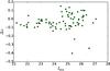 |
Fig. 9 Relation between HST I814 magnitude and the scatter in Δz = (zphot − zspec)/(1 + zspec). An increase in scatter is seen towards fainter I814 magnitudes, highlighting the importance of spectroscopic redshifts for emission-line objects with very faint continuum magnitudes. |
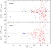 |
Fig. 10 Differences between broad-band magnitudes synthesized from extracted MUSE spectra and filter magnitudes measured by HST; top: V606, bottom: I814. The different symbols represent different object types: blue filled circle denote stars and red open circle stand for galaxies with |
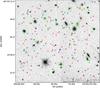 |
Fig. 11 Location of sources with secure redshifts in the HDFS MUSE field. In grey the WFPC2 F814W image. The object categories are identified with the following colours and symbols: blue: stars, cyan: nearby objects with z< 0.3, green: [O ii] emitters, yellow: objects identified solely with absorption lines, magenta: C iii] emitters, orange: AGN, red circles: Lyα emitters with HST counterpart, red triangles: Lyα emitters without HST counterpart. Objects which are spatially extended in MUSE are represented by a symbol with a size proportional to the number of spatially resolved elements. |
4.6. Spectrophotometric accuracy
The spectral range of MUSE coincides almost perfectly with the union of the two HST/WFPC2 filters F606W and F814W. It is therefore possible to synthesize broad-band magnitudes in these two bands directly from the extracted spectra, without any extrapolation or colour terms. In principle, a comparison between synthetic MUSE magnitudes with those measured in the HST images, as provided by Casertano et al. (2000), should give a straightforward check of the overall fidelity of the spectrophotometric calibration. In practice such a comparison is complicated by the non-negligible degree of blending and other aperture effects, especially for extended sources but also for the several cases of multiple HST objects falling into one MUSE seeing disk. We have therefore restricted the comparison to stars and compact galaxies with spatial  (as listed by Casertano et al., 2000). We also remeasured the photometry in the HST data after convolving the images to MUSE resolution, to consistently account for object crowding.
The outcome of this comparison is shown in Fig. 10, for both filter bands. Considering only the 8 spectroscopically confirmed stars in the field (blue dots in Fig. 10), all of which are relatively bright and isolated, Star ID#0 is partly saturated in the HST images and consequently appears 1 mag brighter in MUSE than in HST. For the remaining 7 stars, the mean magnitude differences (MUSE − HST) are +0.05 mag in both bands, with a formal statistical uncertainty of ±0.04 mag. The compact galaxies (red dots in Fig. 10) are much fainter on average, and the MUSE measurement error at magnitudes around 28 or fainter is probably dominated by flat fielding and background subtraction uncertainties. Nevertheless, the overall flux scales are again consistent. We conclude that the spectrophotometric calibration provides a flux scale for the MUSE data cube that is fully consistent with external space based photometry, at least for sources with V606 brighter than 28 mag.
5. Census of the MUSE HDFS field
Given the data volume, its 3D information content and the number of objects found, it would be prohibitive to show all sources in this paper. Instead, detailed informations content for all objects will be made public as described in Appendix B. In this section we carry out a first census of the MUSE data cube with a few illustrations on a limited number of representative objects.
A total of 189 objects in the data cube have a securely determined redshift. It is a rich content with 8 stars and 181 galaxies of various categories. Table 1 and Fig. 11 give a global view of the sources in the field. The various categories of objects are described in the following subsections.
Census of the objects in the MUSE HDFS field sorted by categories.
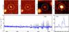 |
Fig. 12 ID#160 is a z = 1.28 [O ii] emitter with a faint (I814 ~ 26.7) HST counterpart. The HST images in the F606W and F814W filters are shown at the top left, the MUSE reconstructed white-light and [O ii] continuum subtracted narrow band images at the top right. The one arcsec radius red circles show the object location derived from the HST image. At the bottom left, the full spectrum (in blue), smoothed with a 4 Å boxcar, and its 3σ error (in grey) are displayed. A zoom of the unsmoothed spectrum, centred around the [O ii]3726, 3729 emission lines, is also shown at the bottom right. |
5.1. Stars
We obtained spectra for 8 stars in our field. Seven were previously identified by Kilic et al. (2005) from proper motion measurements of point sources in the HDFS field. Among these stars we confirm that HDFS 1444 (ID#18) is a white dwarf. We also identify one additional M star (ID#31) that was not identified by Kilic et al. (2005).
5.2. Nearby galaxies
In the following we refer to objects whose [O ii] emission line is redshifted below the 4800 Å blue cut-off of MUSE as nearby galaxies; that is all galaxies with z< 0.29. Only 7 galaxies fall into this category. Except for a bright (ID#1 V606 = 21.7) and a fainter (ID#26 V606 = 24.1) edge-on disk galaxy, the 5 remaining objects are faint compact dwarfs (V606 ~ 25−26).
5.3. [O II] emitters
A large fraction of identified galaxies have [O ii]3726, 3729 in emission and we will refer to these as [O ii]-emitters in the following even if this is not the strongest line in the spectrum. In Fig. 12 we show an example of a faint [O ii] emitter at z = 1.28 (ID#160). In the HST image it is a compact source with a 26.7 V606 and I814 magnitude.
The average equivalent width of [O ii]3727 is 40 Å in galaxies spanning a wide range in luminosity from dwarfs with MB ≈ −14 to the brightest galaxy at MB ≈ −21.4, and sizes from marginally resolved to the largest (ID#4) with an extent of 0.9′′ in the HST image.
It is also noticeable that the [O ii]-emitters often show significant Balmer absorption. In the D4000N–HδA diagram they fall in the region of star forming and post-starburst galaxies. This frequent strong Balmer absorption does fit with previous results from the GDDS (Le Borgne et al., 2007) and VVDS (Wild et al., 2009) surveys.
5.4. Absorption line galaxies
For 10 galaxies, ranging from z = 0.83 to z = 3.9, the redshift determination has been done only on the basis of absorption lines. This can be rather challenging for faint sources because establishing the reality of an absorption feature is more difficult than for an emission line. For that reason the faintest source with a secure absorption line redshift has I814 = 26.2 and z = 3.9, while the faintest source (ID#83) with absorption redshifts in the 1.5 <z< 2.9 so-called MUSE “redshift desert” (Steidel et al., 2004) has I814 of 25.6.
A notable pair of objects is ID#50 and ID#55 which is a merger at z = 2.67 with a possible third companion based on the HST image, which can not be separated in the MUSE data. And while not a pure absorption line galaxy, as it does have [O ii]3727 in emission, object ID#13 shows very strong MgiiandFe ii absorption lines.
5.5. C III] emitters
At 1.5 <z< 3, well into the “redshift desert”, the main emission line identified is C iii]1907, 1909, which is typically resolved as a doublet of emission lines at the resolution achieved with MUSE. Among the clear C iii] emitters identified, the most interesting one (ID#97) is displayed in Fig. 13. It is a z = 1.57 galaxy with strong C iii]1907, 1909 and Mg ii 2796, 2803 emission lines. It appears as a compact source in the HST images with V606 = 26.6 and I814 = 25.8. The object is unusually bright in C iii] with a total flux of 2.7 × 10⁻¹⁸ erg s-1 cm-2 and a rest-frame equivalent width of 16 Å. These are relatively rare objects, with only 17 found in our field of view, but such C iii] emission is expected to appear for younger and lower mass galaxies, typically showing a high ionization parameter (Stark et al., 2014).
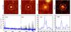 |
Fig. 13 ID#97 is a z = 1.57 strong C iii] emitter. The HST images in F606W and F814W filters are shown at the top left, the MUSE reconstructed white-light, the C iii] and Mg ii continuum subtracted narrow band images at the top right. The one arcsec radius red circles show the object location derived from the HST image. At the bottom left, the full spectrum (in blue), smoothed with a 4 Å boxcar, and its 3σ error (in grey) are displayed. A zoom of the unsmoothed spectrum, centred around the C iii]1907, 1909 Å and Mg ii 2796, 2803 Å emission lines, are also shown at the bottom right. |
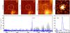 |
Fig. 14 ID#553 is a z = 5.08 Lyα emitter without HST counterpart. The HST images in F606W and F814W filters are shown at the top left, the MUSE reconstructed white-light and Lyα narrow band images at the top right. The one arcsec radius red circles show the emission line location. The spectrum is displayed on the bottom figures; including a zoom at the emission line. At the bottom left, the full spectrum (in blue), smoothed with a 4 Å boxcar, and its 3σ error (in grey) are displayed. A zoom of the unsmoothed spectrum, centred around the Lyα emission line, is also shown at the bottom right. |
5.6. Lyα emitters
The large majority of sources at z > 3 are identified through their strong Lyman-α emission line. Interestingly, 26 of the discovered Lyα emitters are below the HST detection limit, i.e. V606 > 29.6 and I814 > 29 (3σ depth in a 0.2 arcsec2 aperture, Casertano et al. 2000). Approximately 60% of them have a high S/N and exhibit the typical asymmetric Lyα profile. We produced a stacked image in the WFPC2-F814W filter of these 26 Lyα emitters not individually detected in HST and measured an average continuum at the level of I814 = 29.8 ± 0.2 AB (Drake et al., in prep.). We present in Fig. 14 one such example, ID#553 in the catalogue. With a total Lyα flux of 4.2 × 10⁻¹⁸ erg s-1 cm-2 the object is one of the brightest of its category. It is also unambiguously detected in the reconstructed Lyα narrow band image. With such a low continuum flux the emission corresponds to a rest-frame equivalent width higher than 130 Å.
Note that we have found several even fainter line emitters that have no HST counterpart. However, because of their low S/N, it is difficult to firmly identify the emission line and they have therefore been discarded from the final catalogue.
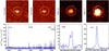 |
Fig. 15 Example of spatially overlapping objects: a z = 3.09 Lyα emitter (ID#71) with a z = 0.83 [OII] emitter (ID#72). The HST images in F606W and F814W filters are shown at the top left, the MUSE Lyα and [O ii] images at the top right. The one arcsec radius red circles show the object location derived from the HST image. At the bottom left, the full spectrum (in blue), smoothed with a 4 Å boxcar, and its 3σ error (in grey) are displayed. A zoom of the unsmoothed spectrum, centred around the Lyα and [O ii]3727 emission line, is also shown at the bottom right. |
5.7. Active galactic nuclei
Among the [O ii] emitting galaxies we identify two objects (ID#10 and ID#25) that show significant [Ne v] 3426 emission, a strong signature of nuclear activity. Both galaxies show pronounced Balmer breaks and post-starburst characteristics, and their forbidden emission lines are relatively broad with a FWHM ~230 km s-1. There is, however, no clear evidence for broader permitted lines such as Mg ii 2798, thus both objects are probably type 2 AGN. Both objects belong to the same group of galaxies at z ≃ 1.284 (Sect. 6.2).
Object ID#144 was classified by Kilic et al. (2005) as a probable QSO at z = 4.0 on the basis of its stellar appearance and its UBVI broad band colours. The very strong Lyα line of this objects confirms the redshift (z = 4.017), but as the line is relatively narrow (~100 km s-1) and no other typical QSO emission lines are detected, a definite spectroscopic classification as an AGN is not possible.
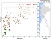 |
Fig. 16 Redshift distribution of sources in the HDFS MUSE field. Left: redshift versus HST I814AB magnitude. The symbol size is proportional to the object’s HST size. The green circles are for the published spectroscopic redshifts and the brown symbols for the new MUSE measurements. The red arrows show objects without HST counterparts. The dashed line shows the 3σ detection limit for the HST F814W images. Right: the grey histogram shows the distribution of all magnitudes in the HST catalogue while the light blue histogram shows the magnitude distribution of those galaxies with confirmed redshifts and HST counterparts. The last histogram bar centred at I814 = 29.75 is for the Lyα emitters not detected in the HST image. The blue curve gives the completeness of the redshift identification with respect to the identified sources in the HST images. |
5.8. Spatially resolved galaxies
Twenty spatially resolved galaxies up to z ~ 1.3 are identified in the MUSE data cube (see Fig. 11). We consider a galaxy as resolved if it extends over a minimum area of twice the PSF. To compute this area we performed emission line fitting (see Sect. 7) on a list of 33 galaxies that had previously been identified to be extended in the HST images. Flux maps were built for each fitted emission line and we computed the galaxy size (FWHM of a 2D fitted Gaussian) using the brightest one (usually [O ii]). Among these 20 resolved galaxies, 3 are at low redshift (z ≤ 0.3) and 4 are above z ~ 1. Note that 5 of the resolved galaxies are in the group identified at ~0.56 (see Sect. 6.2) including ID#3 which extends over ~5 times the MUSE PSF.
5.9. Overlapping objects
While searching for sources in the MUSE data cube, we encountered a number of spatially overlapping objects. In many cases a combination of high spatial resolution HST images and MUSE narrow-band images has been sufficient to assign spectral features and redshifts to a specific galaxy in the HST image. But in some cases, the sources cannot be disentangled, even at the HST resolution. This is illustrated in Fig. 15, where the HST image shows only one object but MUSE reveals it to be the result of two galaxies that are almost perfectly aligned along the line of sight: an [O ii] emitter at z = 0.83 and a z = 3.09 Lyα emitter. There are other cases of objects that potentially could be identified as mergers on the basis of the HST images but are in fact just two galaxies at different redshifts. The power of the 3D information provided by MUSE is nicely demonstrated by these examples.
6. Redshift distribution and global properties
6.1. Redshift distribution
We have been able to measure a redshift at confidence ≥1 for 28% of the 586 sources reported in HST catalogue of Casertano et al. (2000) in the MUSE field. The redshift distribution is presented in Fig. 16. We reach 50% completeness with respect to the HST catalogue at I814 = 26. At fainter magnitudes the completeness decreases, but it is still around 20% at I814 = 28. In addition to the sources identified in the HST images, we found 26 Lyα emitters, i.e. 30% of the entire Lyα emitter sample, that have no HST counterparts and thus have I814 > 29.5.
Redshifts are distributed over the full z = 0−6.3 range. Note the decrease in the z = 1.5−2.8 window – the well known redshift desert – corresponding to the wavelengths where [O ii] is beyond the 9300 Å red limit of MUSE and Lyα is bluer than the 4800 Å blue cut-off of MUSE.
Although the MUSE HDFS field is only a single pointing, and thus prone to cosmic variance, one can compare the measured redshift distribution with those from other deep spectroscopic surveys (e.g. zCOSMOS-Deep – Lilly et al. 2007; Lilly et al. 2009, VVDS-Deep – Le Fèvre et al. 2013, VUDS – Le Fevre et al. 2015). The latter, with 10 000 galaxies in the z ~ 2−6 range, is the most complete.
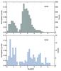 |
Fig. 17 Comparison of the HDFS-MUSE normalized redshift distribution (bottom) with the one from the VUDS (top). |
We show in Fig. 17 the MUSE-HDFS and VUDS normalized redshift distributions. They look quite different. This was expected given the very different observational strategy: the VUDS redshift distribution is the result of a photometric redshift selection zphot > 2.3 ± 1σ (with first and second peaks of PDF) combined with continuum selection IAB < 25, while MUSE does not make any pre-selection. With 22% of galaxies at z > 4 in contrast to 6% for the VUDS, MUSE demonstrates a higher efficiency for finding high redshift galaxies. The number density of observed galaxies is also very different between the two types of observations. With 6000 galaxies per square degree, the VUDS is the survey which achieved the highest density with respect to the other spectroscopic surveys (see Fig. 30 of Le Fevre et al. 2015). This translates, however, to only 1.7 galaxies per arcmin2, which is two orders of magnitude smaller than the number density achieved by MUSE in the HDFS.
6.2. Galaxy groups
The high number density of accurate spectroscopic redshifts allows us to search for galaxy groups in the field. We applied a classical friend-of-friend algorithm to identify galaxy groups, considering only secure redshifts in our catalogue, i.e. those with confidence index ≥1. We adopted a maximum linking length Δr of 500 kpc in projected distance and Δv = 700 km s-1 in velocity following the zCosmos high redshift group search by Diener et al. (2013). The projected distance criterium has very little influence since our field-of-view of 1′ on a side corresponds to ~500 kpc at most. This results in the detection of 17 groups with more than three members. These are listed in Table 2 together with their richness, redshift, and nominal rms size and velocity dispersion as defined in Diener et al. (2013).
Among the 181 galaxies with a secure redshift in our catalogue, 43% reside in a group, 29% in a pair and 28% are isolated. The densest structure we find lies at z = 1.284 and has nine members, including 2 AGN and an interacting system showing a tidal tail, all concentrated to the north west of the field. The structure at z ~ 0.578 first spotted by Vanzella et al. (2002) and further identified as a rich cluster by Glazebrook et al. (2006) shows up here as a 5-member group. The richer group (6 members) at slightly lower redshift (z = 0.565) is also within the redshift range 0.56−0.60 considered by Glazebrook et al. (2006) and could be part of the same large scale structure. The highest redshift group identified is also the one with the lowest vrms of all groups: three Ly-α emitters at z = 5.71 within 26 km s-1. We also find two relatively rich groups both including six members at redshift ~4.7 and ~4.9.
Galaxy groups detected in the HDFS ordered by redshift.
6.3. Number counts of emission line galaxies
With more than 100 emission line galaxies identified by MUSE in this field, a meaningful comparison of the observed number counts with expectations from the literature is possible. We consider Lyα and [O ii]3727 emitters.
While integrated emission line fluxes can, in principle, be measured easily from the fits to the extracted spectra (see Appendix A), the significant level of crowding among faint sources resulted in extraction masks that were often too small for capturing the total fluxes. This is especially relevant for Lyα emitters which in many cases show evidence for extended line emission. In order to derive robust total fluxes of [O ii] and Lyα emitters we therefore adopted a more manual approach. We first produced a “pure emission line cube” by median-filtering the data in spectral direction and subtracted the filtered cube. We then constructed narrow-band images centred on each line, which were now empty of sources except for the emitters of interest. Finally, total line fluxes were determined by a growth curve analysis in circular apertures around each source. We adjusted the local sky background for each line such that the growth curve became flat within ~2′′ from the centroid, and integrated the emission line flux inside that aperture. Avoiding the edges of the field, this procedure yielded subsamples of 74 Lyα and 41 [O ii] emitters, with well-measured emission line fluxes.
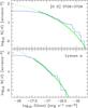 |
Fig. 18 Cumulative number counts of emission line galaxies in the HDFS, as a function of line flux. Top panel: [O ii] emitters; bottom panel: Lyα emitters. The green lines show the predictions for the relevant redshift ranges (0.288 <z< 1.495 and 2.95 <z< 6.65, respectively), using a compilation of published luminosity functions as described in the text. |
The resulting number counts of the two object classes, expressed as the cumulative number of objects per arcmin2 brighter than a given flux, are depicted by the blue step functions in Fig. 18. Both panels show a relatively steep increase at bright fluxes which then flattens and eventually approaches a constant number density for line fluxes of f ≲ 2 × 10-18 erg s-1 cm-2, as no fainter objects are added to the sample. The detailed shapes of these curves depend on the emission line luminosity function and its evolution with redshift, but also on the selection functions which are different for the present samples of Lyα and [O ii] emitters. A detailed discussion of this topic is beyond the scope of this paper. We note that at 5 × 10-18 erg s-1 cm-2, the numbers of detected Lyα and[O ii] emitters are equal; at fainter flux levels, Lyα emitters are more numerous than [O ii] emitters.
Contrasting the MUSE results for the HDFS to expectations from the literature is not straightforward, as the relevant surveys have very diverse redshift coverages. In the course of MUSE science preparations, we combined several published results into analytic luminosity functions for both Lyα and [O ii] emitters, which we now compare with the actual measurements. For the statistics of [O ii] emitters we used data by Ly et al. (2007), Takahashi et al. (2007), and Rauch et al. (2008), plus some guidance from the predictions for Hα emitters by Geach et al. (2010). For the Lyα emitters we adopted a luminosity function with non-evolving parameters following Ouchi et al. (2008), with luminosity function parameters estimated by combining the Ouchi et al. (2008) results with those of Gronwall et al. (2007) and again Rauch et al. (2008). Note that these luminosity functions are just intended to be an overall summary of existing observations, and no attempt was made to account for possible tensions or inconsistencies between the different data sets.
Figure 18 shows the predicted cumulative number counts based on these prescriptions as solid green curves (dotted where we consider these predictions as extrapolations). While the overall match appears highly satisfactory, cosmic variance is of course a strong effect in a field of this size, particularly at the bright end. We reiterate that any more detailed comparison with published luminosity functions would be premature. Nevertheless, it is reassuring to see that the present MUSE source catalogue for the HDFS gives number counts consistent with previous work.
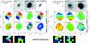 |
Fig. 19 Morpho-kinematics of HDFS5140 (left) and HDFS4070 (right). For each galaxy and from left to right. Top: HST/WFPC2 F814W image in log scale (the yellow rectangle shows the GIRAFFE FoV), the MUSE [O iii]λ5007 flux map, and the deconvolved [O iii]λ5007 flux map from GalPaK3D (for HDFS5140 only). Middle: MUSE observed velocity field from Hβ and [O iii], velocity field of the 2D rotating disk model, residual velocity field, and deconvolved [O iii]λ5007 velocity field from GalPaK3D (for HDFS5140 only). Bottom: MUSE observed velocity dispersion map from Hβ and [O iii], velocity dispersion map deduced from the 2D velocity field model (beam-smearing effect and spectral PSF), deconvolved velocity dispersion map, and deconvolved [O iii]λ5007 velocity dispersion from GalPaK3D (for HDFS5140 only). In each map, north is up and east is left. The centre used for kinematical modelling is indicated as a white cross, the position angle is indicated by the black line which ends at the effective radius. For comparison, the published velocity field and dispersion map obtained with GIRAFFE for HDFS5140 (Puech et al., 2006) and HDFS4070 (Flores et al., 2006) are shown in the bottom row. |
7. Spatially resolved kinematics
To illustrate the power of MUSE for spatially-resolved studies of individual galaxies, we derive the kinematics for two galaxies with published spatially-resolved spectroscopy. These galaxies, namely ID#6 (hereafter HDFS4070) at z = 0.423 and ID#9 (hereafter HDFS5140) at z = 0.5645, were observed earlier with the GIRAFFE multi-IFU at the VLT as part of the IMAGES survey (Flores et al. 2006; Puech et al. 2006). These observations have a spectral resolution of 22−30 km s-1, were taken with a seeing in the 0.35−0.8″ range and used an integration time of 8 h.These data have mainly been used to derive the ionized gas kinematics from the [O ii] emission lines, which was published in Flores et al. (2006) and Puech et al. (2006) for HDFS4070 and HDFS5140, respectively. As shown in the lower panels of Fig. 19, the velocity fields appear very perturbed. This led those authors to conclude that these galaxies show complex gas kinematics.
With the MUSE data in hand, we have the opportunity to revisit the ionized gas kinematics for these two galaxies and to compare the derived parameters with those obtained with GIRAFFE. To probe the gas kinematics, we make use of the three brightest emission lines available in the MUSE spectral range: the [O ii] doublet, Hβ, and [O iii].
The flux and velocity maps are presented in Fig. 19. Rotating disk models, both in 2D (see Epinat et al. 2012 for details) and with GalPaK3D (Bouché et al. 2013, 2014) are also shown. Compared to the GIRAFFE maps, the kinematics revealed by MUSE give a very different picture for these galaxies.
The barred structure of HDFS4070 is clearly detected in the MUSE velocity field with its typical S-shape, whereas the velocity field of HDFS5140 is much more regular and typical of an early-type spiral with a prominent bulge. The maximum rotation velocity derived for HDFS5140 is consistent between the 2D and 3D models (~140 km s-1), but is significantly lower than the value (~220 km s-1) obtained from the GIRAFFE data. In HDFS4070, the velocity dispersion is quite uniform over the disk whereas it is clearly peaked at the centre of HDFS5140. Note, however, that there are some structures in the velocity dispersion residual map of this galaxy, with velocity dispersion of the order of ~80−100 km s-1. Such a broad component, aligned along the south-west side of the minor axis of HDFS5140, could well be produced by superwind-driven shocks as revealed in a significant population of star-forming galaxies at z ~ 2 (see e.g. Newman et al. 2012). Note that outflows were already suspected in this galaxy from the GIRAFFE data, but not for the same reasons. Puech et al. (2006) argued that the velocity gradient of HDFS5140 is nearly perpendicular to its main optical axis, which is clearly not the case.
The quality of the 2D MUSE maps uniquely enables reliable modelling and interpretation of the internal physical properties of distant galaxies. A complete and extensive analysis of galaxy morpho-kinematics probed with MUSE in this HDFS field will be the scope of a follow-up paper (Contini, in prep.).
8. Summary and conclusion
The HDFS observations obtained during the last commissioning run of MUSE demonstrate its capability to perform deep field spectroscopy at a depth comparable to the HST deep photometry imaging.
In 27 h, or the equivalent of 4 nights of observations with overhead included, we have been able to get high quality spectra and to measure precise redshifts for 189 sources (8 stars and 181 galaxies) in the 1 arcmin2 field of view of MUSE. This is to be compared with the 18 spectroscopic redshifts that had been obtained before for (relatively bright) sources in the same area. Among these 181 galaxies, we found 26 Lyα emitters which were not even detected in the deep broad band WFPC2 images. The redshift distribution is different from the ones derived from deep multi-object spectroscopic surveys (e.g. Le Fevre et al. 2015) and extends to higher redshift. The galaxy redshifts revealed by MUSE extend to very low luminosities, as also shown in Fig. 20. Previous deep optical surveys like those of Stark et al. (2010) in the GOODS field did not push to such faint magnitudes. Stark et al. obtained emission line redshifts to AB = 28.3 and it can be seen that MUSE can be used to derive Lyα fluxes and redshifts to fainter limits. We achieved a completeness of 50% of secure redshift identification at I814 = 26 and about 20% at I814 = 27−28.
In the MUSE field of view, we have detected 17 groups with more than three members. The densest group lies at z = 1.284 and has nine members, including 2 AGN and an interacting system showing a tidal tail. We also find three groups of Lyα emitters at high redshifts (z ~ 4.7, 4.9 and 5.7).
We have also investigated the capability of MUSE for spatially resolved spectroscopy of intermediate redshift galaxies. Thanks to its excellent spatial resolution, MUSE enables reliable modelling and interpretation of the internal physical properties of distant galaxies. Although the number of objects with relevant spatial information is limited to twenty in the MUSE HDFS field, this is still a large multiplex factor compared to single object pointing observations used e.g. for the MASSIV survey (Contini et al., 2012) with SINFONI at the VLT.
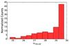 |
Fig. 20 Relative counts of MUSE HDFS Lyα emitters (in %) versus UV continuum magnitude. Note that the last bin of the histogram contains the 12 Lyα emitters with magnitude 29.25 <I814< 29.75 (taken from Casertano et al. 2000, catalogue) and the 26 MUSE Lyα emitters not detected by HST which have been arbitrarily assigned the average magnitude estimated from the stacked image I814 = 29.5 (see Sect. 5.6). |
The MUSE observations of the HDFS are already among the deepest spectroscopic survey ever performed in optical astronomy. It is a unique data set and can be used for a wide range of follow-up studies. We release the reduced data world-wide, and make the associated products public (see Appendix B).
The unique performance in ultra-deep spectroscopic fields achieved by MUSE is very complementary to wide field multi-object spectroscopic surveys (e.g. Le Fevre et al. 2015). The latter cover a much larger field of view and is much more efficient to probe the bright end of the continuum luminosity function while MUSE can probe the faint end of emission line luminosity function where the blind selection is a great helper. In addition MUSE is able to obtain several hundred redshifts per arcmin2 in a moderate amount of time, a spatial density two orders of magnitude higher than what is achieved by current multi-object spectroscopic surveys.
With its capability to obtain high quality spectroscopic information of the population of faint galaxies at high-redshift without having to perform any pre-selection, MUSE is also highly complementary to the present (Hubble, ALMAs) and future (James Webb) ultra-deep surveys. As we have demonstrated using the HDFS observations, MUSE has in addition its own large potential for discoveries. MUSE is not limited to follow-up observations, but is also able to find large number of objects that are not (or barely) detected by broad band deep imaging.
These observations performed during the commissioning mark the end of the realization of the instrument and the start of the science exploitation. This is, however, only the first step. Further improvements of the data reduction process – such as super flat-fields or optimal combination of exposures – are still possible and will be implemented in the near future. We are also developing new methods for 3D source detections, optimised for the large size of the MUSE data cubes (Paris et al. 2013; Herenz, in prep.; Meillier, in prep.; Cantalupo, in prep.). With these new tools and an improved data reduction, we expect to further extend the number of secure redshift identifications in the field. This will be the subject of a future public release for the HDFS field.
Another major milestone is expected in a few years, when the Adaptive Optics Facility will come in operations at UT4 (Arsenault et al., 2012). The four laser guide stars, the deformable VLT secondary mirror and GALACSI, the module dedicated to MUSE (Ströbele et al., 2012), will improve the spatial resolution of MUSE up to 50% without impacting its superb throughput and efficiency.
Online material
Appendix A: Catalogue
Table A.1 lists the basic properties of the galaxies studied in the paper. All the sources from the Casertano et al. (2000) catalogue that fall within the field of view of the final MUSE data cube are included as well as sources without an entry in the Casertano et al. catalogue. Note that F814W magnitudes have been manually computed for a few objects that were missing in the Casertano et al. (2000) catalogue but were clearly present in the HST image. The table is sorted by increasing apparent F814W magnitude from the catalogue with no particular ordering of the sources without a catalogue magnitude.
The first column gives a running number which is the one used for ID#XX entries in the text. The subsequent two columns give the right ascenscion and declination from the MUSE observations, then follows the F814 SExtractor BEST magnitude from the Casertano et al. catalogue and the F606W − F814W colour from the BEST magnitudes. The redshift and its confidence follows thereafter, with the subsequent column indicating features identified in the spectrum. The final column gives the running number of the object in the Casertano et al. catalogue.
The second-to-last column, Nexp, gives the median number of exposures going into the reduction of the region where the spectrum was extracted. Recall that the exposures are 30 min in duration, so a value of 40 corresponds to an exposure time of 20 h. Our redshift catalogue is naturally less complete where Nexp < 30.
Table A.2 gives the emission line fluxes measures off the 1D spectra produced by straight summation. In this table only the 181 sources with redshift >0 with redshift confidence ≥1 are included. The procedure adopted for emission line flux measurements is given in Sect. 4.3. Note that the fluxes have been corrected for Galactic reddening using the Schlegel et al. (1998) dust maps using the reddening curve from O’Donnell (1994) for consistency with that work.
We emphasise that there has been no attempt to correct these fluxes to true total fluxes. In particular these fluxes are generally lower than those used in Sect. 6.3 which are aperture corrected. However the technique used in Sect. 6.3 is not suitable for all galaxies so we use the simpler approach here. Note also that the Lyα fluxes have been measured by fitting a Gaussian to an asymmetric line so are likely to give suboptimal flux measurements. Finally observe also that flux measurements are provided for all lines within the wavelength range of the spectrum, regardless of whether they were reliably detected or not.
Table A.3 gives the list of the redshift comparison between MUSE and published spectroscopic redshifts discussed in Sect. 4.4.
Basic data and redshifts on sources with spectra in the HDF-S.
Line fluxes for galaxies with secure redshifts in units of 10-18 erg s-1 cm-2 Å-1.
Redshift comparison.
Appendix B: Public data release
In addition to the source catalogue, we release the reduced data cube and associated files. We also deliver spectra and reconstructed images in the main emission lines for all the catalogue sources4.
The field of view of MUSE is first split in 24 “channels”, each channel is then split again in 48 “slices” by the corresponding image slicer.
A short description is also given in Weilbacher et al. (2012).
All this material is available at http://muse-vlt.eu/science
Acknowledgments
We thank the referee Michele Cirasuolo and Olivier Le Fevre for proving useful comments on the submitted version and Laure Piqueras and Gerard Zins for their support with analysis and observation software. We also warmly thank Fernando Selman and all Paranal staff for their enthusiastic support of MUSE during the commissioning runs. R.B. acknowledges support from the ERC advanced grant 339659-MUSICOS. J.R., B.C., V.P. acknowledge support from the ERC starting grant CALENDS. T.C., B.G., A.D. acknowledge support from the ANR FOGHAR. L.M. acknowledges support from the Lyon Institute of Origins under grant ANR-10-LABX-66. S.J.L. and K.S. acknowledge support from the Swiss National Science Foundation.
References
- Arsenault, R., Madec, P.-Y., Paufique, J., et al. 2012, SPIE Conf. Ser., 8447 [Google Scholar]
- Bacon, R., Accardo, M., Adjali, L., et al. 2010, SPIE Conf. Ser., 7735, 8 [Google Scholar]
- Bacon, R., Vernet, J., Borosiva, E., et al. 2014, The Messenger, 157, 21 [Google Scholar]
- Beckwith, S. V. W., Stiavelli, M., Koekemoer, A. M., et al. 2006, AJ, 132, 1729 [NASA ADS] [CrossRef] [Google Scholar]
- Bertin, E., & Arnouts, S. 1996, A&AS, 117, 393 [NASA ADS] [CrossRef] [EDP Sciences] [Google Scholar]
- Bouché, N., Murphy, M. T., Kacprzak, G. G., et al. 2013, Science, 341, 50 [NASA ADS] [CrossRef] [Google Scholar]
- Brammer, G. B., van Dokkum, P. G., & Coppi, P. 2008, ApJ, 686, 1503 [NASA ADS] [CrossRef] [Google Scholar]
- Brinchmann, J., Charlot, S., White, S. D. M., et al. 2004, MNRAS, 351, 1151 [NASA ADS] [CrossRef] [Google Scholar]
- Carollo, C. M., Bschorr, T. J., Renzini, A., et al. 2013, ApJ, 773, 112 [NASA ADS] [CrossRef] [Google Scholar]
- Casertano, S., de Mello, D., Dickinson, M., et al. 2000, AJ, 120, 2747 [NASA ADS] [CrossRef] [Google Scholar]
- Chen, H.-W., Fernandez-Soto, A., Lanzetta, K. M., et al. 1998 [arXiv:astro-ph/9812339] [Google Scholar]
- Contini, T., Garilli, B., LeFèvre, O., et al. 2012, A&A, 539, A91 [NASA ADS] [CrossRef] [EDP Sciences] [Google Scholar]
- Das, P. K. 1991, Optical Signal Processing – Fundamentals (Berlin, Heidelberg, New York: Springer) [Google Scholar]
- Diener, C., Lilly, S. J., Knobel, C., et al. 2013, ApJ, 765, 109 [NASA ADS] [CrossRef] [Google Scholar]
- Epinat, B., Tasca, L., Amram, P., et al. 2012, A&A, 539, A92 [NASA ADS] [CrossRef] [EDP Sciences] [Google Scholar]
- Ferguson, H. C., Dickinson, M., & Williams, R. 2000, ARA&A, 38, 667 [NASA ADS] [CrossRef] [Google Scholar]
- Flores, H., Hammer, F., Puech, M., Amram, P., & Balkowski, C. 2006, A&A, 455, 107 [NASA ADS] [CrossRef] [EDP Sciences] [Google Scholar]
- Geach, J. E., Cimatti, A., Percival, W., et al. 2010, MNRAS, 402, 1330 [NASA ADS] [CrossRef] [Google Scholar]
- Glazebrook, K., Verma, A., Boyle, B., et al. 2006, AJ, 131, 2383 [NASA ADS] [CrossRef] [Google Scholar]
- Gronwall, C., Ciardullo, R., Hickey, T., et al. 2007, ApJ, 667, 79 [NASA ADS] [CrossRef] [Google Scholar]
- Horne, K. 1986, PASP, 98, 609 [NASA ADS] [CrossRef] [EDP Sciences] [Google Scholar]
- Ilbert, O., Capak, P., Salvato, M., et al. 2009, ApJ, 690, 1236 [NASA ADS] [CrossRef] [Google Scholar]
- Ilbert, O., McCracken, H. J., Le Fèvre, O., et al. 2013, A&A, 556, A55 [NASA ADS] [CrossRef] [EDP Sciences] [Google Scholar]
- Iwata, I., Inoue, A. K., & Burgarella, D. 2005, A&A, 440, 881 [NASA ADS] [CrossRef] [EDP Sciences] [Google Scholar]
- Kilic, M., Mendez, R. A., von Hippel, T., & Winget, D. E. 2005, ApJ, 633, 1126 [NASA ADS] [CrossRef] [Google Scholar]
- Kausch, W., Noll, S., Smette, A., et al. 2015, A&A, in press DOI: 10.1051/0004-6361/201423909 [Google Scholar]
- Labbé, I., Franx, M., Rudnick, G., et al. 2003, AJ, 125, 1107 [NASA ADS] [CrossRef] [Google Scholar]
- Labbé, I., Huang, J., Franx, M., et al. 2005, ApJ, 624, L81 [NASA ADS] [CrossRef] [Google Scholar]
- Le Borgne, J. F., Paschke, A., Vandenbroere, J., et al. 2007, A&A, 476, 307 [NASA ADS] [CrossRef] [EDP Sciences] [Google Scholar]
- Le Fèvre, O., Cassata, P., Cucciati, O., et al. 2013, A&A, 559, A14 [NASA ADS] [CrossRef] [EDP Sciences] [Google Scholar]
- Le Fevre, O., Tasca, L. A. M., Cassata, P., et al. 2015, A&A, in press, DOI: 10.1051/0004-6361/201423829 [Google Scholar]
- Lee, B., Giavalisco, M., Williams, C. C., et al. 2013, ApJ, 774, 47 [NASA ADS] [CrossRef] [Google Scholar]
- Lilly, S. J., Le Fèvre, O., Renzini, A., et al. 2007, ApJS, 172, 70 [NASA ADS] [CrossRef] [Google Scholar]
- Lilly, S. J., Le Brun, V., Maier, C., et al. 2009, ApJS, 184, 218 [Google Scholar]
- Ly, C., Malkan, M. A., Kashikawa, N., et al. 2007, ApJ, 657, 738 [NASA ADS] [CrossRef] [Google Scholar]
- Mortlock, A., Conselice, C. J., Hartley, W. G., et al. 2013, MNRAS, 433, 1185 [NASA ADS] [CrossRef] [Google Scholar]
- Muzzin, A., Marchesini, D., Stefanon, M., et al. 2013, ApJ, 777, 18 [NASA ADS] [CrossRef] [Google Scholar]
- Newman, S. F., Genzel, R., Förster-Schreiber, N. M., et al. 2012, ApJ, 761, 43 [NASA ADS] [CrossRef] [Google Scholar]
- O’Donnell, J. E. 1994, ApJ, 422, 158 [NASA ADS] [CrossRef] [Google Scholar]
- Ouchi, M., Shimasaku, K., Akiyama, M., et al. 2008, ApJS, 176, 301 [NASA ADS] [CrossRef] [Google Scholar]
- Paris, S., Suleiman, R. F. R., Mary, D., & Ferrari, A. 2013, in Acoustics, Speech and Signal Processing (ICASSP), IEEE Int. Conf., 3947 [Google Scholar]
- Puech, M., Hammer, F., Flores, H., Östlin, G., & Marquart, T. 2006, A&A, 455, 119 [NASA ADS] [CrossRef] [EDP Sciences] [Google Scholar]
- Rauch, M., Haehnelt, M., Bunker, A., et al. 2008, ApJ, 681, 856 [NASA ADS] [CrossRef] [Google Scholar]
- Richard, J., Patricio, V., Martinez, J., et al. 2015, MNRAS, 446, L16 [NASA ADS] [CrossRef] [Google Scholar]
- Rigopoulou, D., Vacca, W. D., Berta, S., Franceschini, A., & Aussel, H. 2005, A&A, 440, 61 [NASA ADS] [CrossRef] [EDP Sciences] [Google Scholar]
- Saracco, P., Fiano, A., Chincarini, G., et al. 2006, MNRAS 367, 349 [NASA ADS] [CrossRef] [Google Scholar]
- Sawicki, M., & Mallén-Ornelas, G. 2003, AJ, 126, 1208 [NASA ADS] [CrossRef] [Google Scholar]
- Schlegel, D. J., Finkbeiner, D. P., & Davis, M. 1998, ApJ, 500, 525 [NASA ADS] [CrossRef] [Google Scholar]
- Smette, A., Sana, H., Noll, S., et al. 2015, A&A, in press, DOI: 10.1051/0004-6361/201423932 [Google Scholar]
- Stark, D. P., Ellis, R. S., Chiu, K., Ouchi, M., & Bunker, A. 2010, MNRAS, 408, 1628 [NASA ADS] [CrossRef] [Google Scholar]
- Stark, D. P., Richard, J., Charlot, S., et al. 2014, MNRAS, submitted [arXiv:1408.3649] [Google Scholar]
- Steidel, C. C., Shapley, A. E., Pettini, M., et al. 2004, ApJ, 604, 534 [NASA ADS] [CrossRef] [Google Scholar]
- Ströbele, S., La Penna, P., Arsenault, R., et al. 2012, SPIE Conf. Ser., 8447 [Google Scholar]
- Takahashi, M. I., Shioya, Y., Taniguchi, Y., et al. 2007, ApJS, 172, 456 [NASA ADS] [CrossRef] [Google Scholar]
- Tremonti, C. A., Heckman, T. M., Kauffmann, G., et al. 2004, ApJ, 613, 898 [NASA ADS] [CrossRef] [Google Scholar]
- van der Wel, A., Franx, M., van Dokkum, P. G., et al. 2014, ApJ, 788, 28 [NASA ADS] [CrossRef] [Google Scholar]
- Vanzella, E., Cristiani, S., Arnouts, S., et al. 2002, A&A, 396, 847 [NASA ADS] [CrossRef] [EDP Sciences] [Google Scholar]
- Weilbacher, P. M., Streicher, O., Urrutia, T., et al. 2012, SPIE Conf. Ser., 8451 [Google Scholar]
- Wild, V., Walcher, C. J., Johansson, P. H., et al. 2009, MNRAS, 395, 144 [NASA ADS] [CrossRef] [Google Scholar]
- Williams, R. E., Blacker, B., Dickinson, M., et al. 1996, AJ, 112, 1335 [NASA ADS] [CrossRef] [Google Scholar]
- Williams, R. E., Baum, S., Bergeron, L. E., et al. 2000, AJ, 120, 2735 [NASA ADS] [CrossRef] [Google Scholar]
- Wuyts, S., van Dokkum, P. G., Franx, M., et al. 2009, ApJ, 706, 885 [NASA ADS] [CrossRef] [Google Scholar]
All Tables
Line fluxes for galaxies with secure redshifts in units of 10-18 erg s-1 cm-2 Å-1.
All Figures
|
Fig. 1 Location of the MUSE field of view within the HDFS F814W image. The star used in the slow guiding system is indicated in red and the brightest star in the field (R = 19.6) in blue. |
| In the text | |
|
Fig. 2 Derived FWHM as function of wavelength from the Moffat fit to the brightest star in the field. |
| In the text | |
|
Fig. 3 Reconstructed white-light image of the combined exposures. The flux scale shown on the right is in 10-21 erg s-1 cm-2 Å-1 pixel-1. Orientation is north(up)-east(left). |
| In the text | |
|
Fig. 4 Overall scaling of pixel noise measured in the cubes as a function of the number of exposures combined, relative to the noise in a single exposure. The solid line represents the ideal |
| In the text | |
|
Fig. 5 Example of the extraction process for objects 5 and 144, at z = 0.58 and z = 4.02 respectively. Top row the left panel: MUSE reconstructed white-light image, while the left panel in the bottom row shows the Lyα narrow-band image. Middle panels: object and sky masks, with the object aperture shown in black and the sky aperture in blue. Part of the final extracted spectrum is shown in the right-hand panel on each row. |
| In the text | |
|
Fig. 6 Comparison between the MUSE (red) and FORS1 spectra of Rigopoulou et al. (2005; blue) for the galaxy ID#13, a strong [O ii] emitter at zMUSE = 1.2902. The strongest spectral features are indicated in black. The grey lines show the position of the sky lines. Upper panel: entire spectra; lower panel: zoom on the rest-frame 2300−2800 Å region, which contains strong MgII and FeII absorption features. |
| In the text | |
|
Fig. 7 Comparison between the MUSE (red) and FORS2 spectra of Iwata et al. (2005; blue) for the galaxy ID#43, a strong Lyα emitter at zMUSE = 3.2925. The strongest spectral features are indicated in black. The grey lines show the position of the sky lines; grey areas show wavelength regions for which no FORS2 spectrum was published. Upper panel: entire spectra; middle and lower panels: zoom on the Lyα and 1380−1550 Å region, respectively; the latter contains strong SiIV absorption features. |
| In the text | |
|
Fig. 8 Comparison of MUSE spectroscopic redshifts with the photometric redshifts of Labbé et al. (2003). Upper panel: distribution of Δz as a function of MUSE zsp with outliers highlighted in red. The error bars shows the uncertainties reported by Labbé et al. The grey shaded area depicts the region outside of which objects are considered outliers. Lower panel: direct comparison of MUSE zsp and Labbé et al. (2003)zph with outliers again highlighted in red. |
| In the text | |
|
Fig. 9 Relation between HST I814 magnitude and the scatter in Δz = (zphot − zspec)/(1 + zspec). An increase in scatter is seen towards fainter I814 magnitudes, highlighting the importance of spectroscopic redshifts for emission-line objects with very faint continuum magnitudes. |
| In the text | |
|
Fig. 10 Differences between broad-band magnitudes synthesized from extracted MUSE spectra and filter magnitudes measured by HST; top: V606, bottom: I814. The different symbols represent different object types: blue filled circle denote stars and red open circle stand for galaxies with |
| In the text | |
|
Fig. 11 Location of sources with secure redshifts in the HDFS MUSE field. In grey the WFPC2 F814W image. The object categories are identified with the following colours and symbols: blue: stars, cyan: nearby objects with z< 0.3, green: [O ii] emitters, yellow: objects identified solely with absorption lines, magenta: C iii] emitters, orange: AGN, red circles: Lyα emitters with HST counterpart, red triangles: Lyα emitters without HST counterpart. Objects which are spatially extended in MUSE are represented by a symbol with a size proportional to the number of spatially resolved elements. |
| In the text | |
|
Fig. 12 ID#160 is a z = 1.28 [O ii] emitter with a faint (I814 ~ 26.7) HST counterpart. The HST images in the F606W and F814W filters are shown at the top left, the MUSE reconstructed white-light and [O ii] continuum subtracted narrow band images at the top right. The one arcsec radius red circles show the object location derived from the HST image. At the bottom left, the full spectrum (in blue), smoothed with a 4 Å boxcar, and its 3σ error (in grey) are displayed. A zoom of the unsmoothed spectrum, centred around the [O ii]3726, 3729 emission lines, is also shown at the bottom right. |
| In the text | |
|
Fig. 13 ID#97 is a z = 1.57 strong C iii] emitter. The HST images in F606W and F814W filters are shown at the top left, the MUSE reconstructed white-light, the C iii] and Mg ii continuum subtracted narrow band images at the top right. The one arcsec radius red circles show the object location derived from the HST image. At the bottom left, the full spectrum (in blue), smoothed with a 4 Å boxcar, and its 3σ error (in grey) are displayed. A zoom of the unsmoothed spectrum, centred around the C iii]1907, 1909 Å and Mg ii 2796, 2803 Å emission lines, are also shown at the bottom right. |
| In the text | |
|
Fig. 14 ID#553 is a z = 5.08 Lyα emitter without HST counterpart. The HST images in F606W and F814W filters are shown at the top left, the MUSE reconstructed white-light and Lyα narrow band images at the top right. The one arcsec radius red circles show the emission line location. The spectrum is displayed on the bottom figures; including a zoom at the emission line. At the bottom left, the full spectrum (in blue), smoothed with a 4 Å boxcar, and its 3σ error (in grey) are displayed. A zoom of the unsmoothed spectrum, centred around the Lyα emission line, is also shown at the bottom right. |
| In the text | |
|
Fig. 15 Example of spatially overlapping objects: a z = 3.09 Lyα emitter (ID#71) with a z = 0.83 [OII] emitter (ID#72). The HST images in F606W and F814W filters are shown at the top left, the MUSE Lyα and [O ii] images at the top right. The one arcsec radius red circles show the object location derived from the HST image. At the bottom left, the full spectrum (in blue), smoothed with a 4 Å boxcar, and its 3σ error (in grey) are displayed. A zoom of the unsmoothed spectrum, centred around the Lyα and [O ii]3727 emission line, is also shown at the bottom right. |
| In the text | |
|
Fig. 16 Redshift distribution of sources in the HDFS MUSE field. Left: redshift versus HST I814AB magnitude. The symbol size is proportional to the object’s HST size. The green circles are for the published spectroscopic redshifts and the brown symbols for the new MUSE measurements. The red arrows show objects without HST counterparts. The dashed line shows the 3σ detection limit for the HST F814W images. Right: the grey histogram shows the distribution of all magnitudes in the HST catalogue while the light blue histogram shows the magnitude distribution of those galaxies with confirmed redshifts and HST counterparts. The last histogram bar centred at I814 = 29.75 is for the Lyα emitters not detected in the HST image. The blue curve gives the completeness of the redshift identification with respect to the identified sources in the HST images. |
| In the text | |
|
Fig. 17 Comparison of the HDFS-MUSE normalized redshift distribution (bottom) with the one from the VUDS (top). |
| In the text | |
|
Fig. 18 Cumulative number counts of emission line galaxies in the HDFS, as a function of line flux. Top panel: [O ii] emitters; bottom panel: Lyα emitters. The green lines show the predictions for the relevant redshift ranges (0.288 <z< 1.495 and 2.95 <z< 6.65, respectively), using a compilation of published luminosity functions as described in the text. |
| In the text | |
|
Fig. 19 Morpho-kinematics of HDFS5140 (left) and HDFS4070 (right). For each galaxy and from left to right. Top: HST/WFPC2 F814W image in log scale (the yellow rectangle shows the GIRAFFE FoV), the MUSE [O iii]λ5007 flux map, and the deconvolved [O iii]λ5007 flux map from GalPaK3D (for HDFS5140 only). Middle: MUSE observed velocity field from Hβ and [O iii], velocity field of the 2D rotating disk model, residual velocity field, and deconvolved [O iii]λ5007 velocity field from GalPaK3D (for HDFS5140 only). Bottom: MUSE observed velocity dispersion map from Hβ and [O iii], velocity dispersion map deduced from the 2D velocity field model (beam-smearing effect and spectral PSF), deconvolved velocity dispersion map, and deconvolved [O iii]λ5007 velocity dispersion from GalPaK3D (for HDFS5140 only). In each map, north is up and east is left. The centre used for kinematical modelling is indicated as a white cross, the position angle is indicated by the black line which ends at the effective radius. For comparison, the published velocity field and dispersion map obtained with GIRAFFE for HDFS5140 (Puech et al., 2006) and HDFS4070 (Flores et al., 2006) are shown in the bottom row. |
| In the text | |
|
Fig. 20 Relative counts of MUSE HDFS Lyα emitters (in %) versus UV continuum magnitude. Note that the last bin of the histogram contains the 12 Lyα emitters with magnitude 29.25 <I814< 29.75 (taken from Casertano et al. 2000, catalogue) and the 26 MUSE Lyα emitters not detected by HST which have been arbitrarily assigned the average magnitude estimated from the stacked image I814 = 29.5 (see Sect. 5.6). |
| In the text | |
Current usage metrics show cumulative count of Article Views (full-text article views including HTML views, PDF and ePub downloads, according to the available data) and Abstracts Views on Vision4Press platform.
Data correspond to usage on the plateform after 2015. The current usage metrics is available 48-96 hours after online publication and is updated daily on week days.
Initial download of the metrics may take a while.