| Issue |
A&A
Volume 575, March 2015
|
|
|---|---|---|
| Article Number | A40 | |
| Number of page(s) | 18 | |
| Section | Cosmology (including clusters of galaxies) | |
| DOI | https://doi.org/10.1051/0004-6361/201424767 | |
| Published online | 18 February 2015 | |
The 0.1 <z < 1.65 evolution of the bright end of the [O ii] luminosity function⋆,⋆⋆
1
Departamento de Fisica Teorica, Universidad Autonoma de
Madrid, 28049
Madrid,
Spain
e-mail:
johan.comparat@uam.es
2
Instituto de Fisica Teorica UAM/CSIC, Madrid, Spain
3
Laboratoire d’Astrophysique de Marseille – LAM, Université
d’Aix-Marseille & CNRS, UMR 7326, 38 rue F. Joliot-Curie, 13388
Marseille Cedex 13,
France
4
CRAL, Observatoire de Lyon, Université Lyon 1,
9 avenue Ch. André,
69561
Saint Genis Laval Cedex,
France
5
Laboratoire d’astrophysique, École Polytechnique Fédérale de
Lausanne (EPFL), Observatoire de Sauverny, 1290
Versoix,
Switzerland
6
CPPM, Université d’Aix-Marseille, CNRS/IN2P3
Marseille,
France
7
Institute for Computational Cosmology, Department of Physics,
University of Durham, South
Road, Durham,
DH1 3LE,
UK
8
Department of Physics, Drexel University,
3141 Chestnut Street,
Philadelphia, PA
19104,
USA
9
Lawrence Berkeley National Laboratory,
1 Cyclotron Road, Berkeley, CA
94720,
USA
10
Institute of Cosmology and Gravitation (ICG),
Dennis Sciama Building, Burnaby Road, Univ. of
Portsmouth, Portsmouth, PO1
3FX, UK
11
CEA, Centre de
Saclay, IRFU, 91191
Gif-sur-Yvette,
France
12
Department of Physics and Astronomy, University of
Utah, 115 S 1400 E,
Salt Lake City, UT
84112,
USA
13
Astronomy Department, University of Florida,
211 Bryant Space Science Center,
Gainesville, FL
32611-2055,
USA
14
Department of Astronomy and Astrophysics, The Pennsylvania State
University, University
Park, PA
16802,
USA
15
Institute for Gravitation and the Cosmos, The Pennsylvania State
University, University
Park, PA
16802,
USA
16
Key laboratory of Optical Astronomy, National Astronomical
Observatories, Chinese Academy of Sciences, 100012
Beijing, PR
China
17
Steward Observatory, University of Arizona,
Tucson, AZ
85721,
USA
18
Center for Astronomy and Astrophysics, Department of Physics and
Astronomy, Shangai Jiao Tong University, 200240
Shangai, PR
China
Received: 7 August 2014
Accepted: 19 December 2014
We present the [Oii] (λλ3729,3726) luminosity function measured in the redshift range 0.1 <z< 1.65 with unprecedented depth and accuracy. Our measurements are based on medium resolution flux-calibrated spectra of emission line galaxies with the visual and near UV FOcal Reducer and low dispersion Spectrograph (FORS2) for the Very Large Telescope (VLT) of the European Southern Observatory (ESO) and with the SDSS-III/BOSS spectrograph. The FORS2 spectra and the corresponding catalog containing redshifts and line fluxes are released along with this paper. In this work we use a novel method to combine these surveys with GAMA, zCOSMOS, and VVDS, which have different target selection, producing a consistent weighting scheme to derive the [Oii] luminosity function. The[Oii] luminosity function is in good agreement with previous independent estimates. The comparison with two state-of-the-art semi-analytical models is good, which is encouraging for the production of mock catalogs of [Oii] flux limited surveys. We observe the bright end evolution over 8.5 Gyr: we measure the decrease of log L∗ from 42.4 erg/s at redshift 1.44 to 41.2 at redshift 0.165 and we find that the faint end slope flattens when redshift decreases. This measurement confirms the feasibility of the target selection of future baryonic acoustic oscillation surveys aiming at observing [Oii] flux limited samples.
Key words: catalogs / surveys / galaxies: luminosity function, mass function / cosmology: observations / galaxies: statistics / galaxies: evolution
Appendix A is available in electronic form at http://www.aanda.org
Catalog of the newly acquired spectroscopic redshifts and Tables of the luminosity functions measured are only available at the CDS via anonymous ftp to cdsarc.u-strasbg.fr (130.79.128.5) or via http://cdsarc.u-strasbg.fr/viz-bin/qcat?J/A+A/575/A40
© ESO, 2015
1. Introduction
In the current Λ cold dark matter (CDM) paradigm, the matter dominated Universe at redshift 1.65 becomes driven by dark energy at z = 0.2 (Planck Collaboration XVI 2014). This is one of the reasons for the great interest in understanding the evolution of the Universe during this time span.
To understand the structural evolution of the Universe during this epoch, we need the largest possible map. Measuring rapidly accurate galaxy positions (redshifts) is crucial to building precise maps. The measurement of the emission-line-based redshifts in the optical domain with ground-based optical spectrographs is the least telescope time-consuming observing mode to build such maps. Luckily, narrow spectroscopic signatures in emission are abundant and enable precise redshift measurements. The strongest emission line in an optical galaxy spectra is the Hαλ 6562 Å emission line. It allows the construction of galaxy maps to redshift 0 <z ≲ 0.53, for example, the Canada-France Redshift Survey (CFRS; Lilly et al. 1995; Tresse & Maddox 1998), or the Galaxy And Mass Assembly (GAMA) survey (Driver et al. 2011; Gunawardhana et al. 2013). The second strongest set of emission lines is [Oiii] (λλ4959,5007) and Hβ, which allows the construction of maps to redshift 0 <z ≲ 1.1, for example the VVDS wide survey (Le Fèvre et al. 2013) or the zCOSMOS survey (Lilly et al. 2009). However, to map the complete range 0 <z< 1.65 with these lines it is necessary to observe spectra in the infrared where the atmosphere is less transparent, i.e., with longer exposure times. The third strongest set of lines is the [Oii] (λλ3729,3726) emission line doublet that allows an accurate redshift estimate throughout the redshift range 0 <z< 1.7. The DEEP2 survey (Newman et al. 2013) measured the redshifts in the range 0.7 <z< 1.4 with the resolved [Oii] doublet.
The [Oii] luminosity function (LF) and its evolution is therefore pivotal for the planning of future spectroscopic surveys, which will target the most luminous [Oii] galaxies until they reach the required density to address the fundamental question of the nature of dark energy.
The [Oii] LFs have been previously derived by Gallego et al. (2002); Ly et al. (2007); Argence & Lamareille (2009); Zhu et al. (2009); Gilbank et al. (2010); Sobral et al. (2013); Ciardullo et al. (2013); Drake et al. (2013). In these analyses (spectroscopy or narrowband photometry), the bright end of the [Oii] LF is, however, not well constrained, in part because either the survey areas are small or the redshift selection is very narrow. With our study we aim to better constrain the bright end of the [Oii] LF by using new deep spectroscopic measurements.
In this study, we gather an [Oii] emission line sample from publicly available data to which we add newly acquired spectroscopy. In Sect. 2, we describe current publicly available [Oii] data and the new flux-calibrated spectroscopic data acquired by ESO VLT/FORS2 and by SDSS-III/BOSS spectrograph. With this combined sample we measure the [Oii] LF in Sect. 3. We also project the LF to inform the planning of future surveys. Finally, we compare our measurement with semi-analytical models in Sect. 4. Although this new sample is suitable for such an analysis, we do not perform a new calibration of the relation [Oii] – star formation rate (SFR) – dust, and leave it for future studies.
Throughout the paper, we quote magnitudes in the AB system (Oke & Gunn 1982) and we provide the measurements in Planck cosmology h = 0.673, Ωm = 0.315, ΩΛ = 0.685, wDark Energy = −1 (see Planck Collaboration XVI 2014).
2. [Oii] spectroscopic data
To measure the LF, we collected publicly available [Oii] flux-calibrated spectroscopy from which no [Oii] LF was previously derived.
2.1. GAMA
The Galaxy and Mass Assembly (GAMA) survey released its spectroscopic data and corresponding catalogs (Driver et al. 2011; Baldry et al. 2014). They provide a magnitude-limited sample (r< 19.8) with spectroscopic redshifts (extending to redshift ~0.4) and [Oii] flux measurements corrected from the aperture on one of their fields of stripe 82 (48 deg2 near αJ2000 ~ 217° and δJ2000 ~ 0; Hopkins et al. 2013). We matched this sample to the stripe 82 deep co-add (Annis et al. 2014) to obtain the u,g,r,i,z optical counterpart of each [Oii] emitter.
2.2. VVDS
The VIMOS VLT Deep Survey (VVDS) final data release (Le Fèvre et al. 2013) provides catalogs and spectra of all observations. We used a restricted set of catalogs where spectroscopic redshifts and the fits of the emission lines on the spectra are provided: the deep and ultra deep observations of the 2h field and the wide observations on the 22h field. Spectral features were measured with the same pipeline as in Lamareille et al. (2009). The u,g,r,i,z optical magnitudes for these samples were taken from the CFHT-LS deep and wide observations (Ilbert et al. 2006; Coupon et al. 2009; Bielby et al. 2012).
To derive the integrated line flux, we converted the measured equivalent width (EW) into a flux density using ![\begin{equation} f_{\lambda}^{\rm total}=-EW_{\rm measured}\; 10^{-(m+48.6)/2.5} \frac{c}{\lambda^2_{\left[\mathrm{O\textrm{\textsc{ii}}}\right]}} {\rm erg\; cm^{-2}\;s^{-1}\; \AA^{-1}} , \end{equation}](/articles/aa/full_html/2015/03/aa24767-14/aa24767-14-eq34.png) (1)where m is the broadband magnitude of the CFHTLS filter containing [Oii] . Table 5 gives the magnitude used as a function of the redshift of the galaxy. We compared this flux density with the one measured in the slit to make sure the discrepancy is on the order of magnitude of an aperture correction, and used ftotal in the LF.
(1)where m is the broadband magnitude of the CFHTLS filter containing [Oii] . Table 5 gives the magnitude used as a function of the redshift of the galaxy. We compared this flux density with the one measured in the slit to make sure the discrepancy is on the order of magnitude of an aperture correction, and used ftotal in the LF.
2.3. zCOSMOS
We used the public zCOSMOS 10 k bright spectroscopic sample on COSMOS field (Scoville et al. 2007b; Lilly et al. 2009), which provides spectroscopic redshifts and fits of the emission lines in the spectra. The corresponding optical photometry was taken from Scoville et al. (2007a); Ilbert et al. (2009). The zCOSMOS survey provides the correction of the aperture correction for 1 arcsecond slits along the dispersion axis.
2.4. New data from ESO/VLT on the COSMOS field
The data described in this section is thoroughly documented and publicly available1. We constructed an optimized color-box using the extremely rich ground-based photometry of the COSMOS/HST-ACS field (Capak et al. 2007; Scoville et al. 2007a; Ilbert et al. 2009) in order to target galaxies with strong emission lines that are expected in the redshift range 0.9 <z< 1.7.
We observed 2265 targets with the VLT/FORS-2 instrument equipped with the 600z+23 holographic grating, which is the unique multi-object spectroscopic ESO instrument that reaches out to 1 μm allowing one to probe galaxies with redshift z ≲ 1.7 using the [Oii] emission line. The spectral range 737 nm–1070 nm is sampled with a resolution λ/ Δλ = 1390 at 900 nm. We made two short exposures of 309 s each and we observed emission lines with a flux > 10-16 erg s-1 cm-2 at a signal-to-noise ratio (S/N) > 7 at redshift z> 1.3 and with a better S/N at lower redshift.
The targets are on the COSMOS field centered at RAJ2000 = 150° and DecJ2000 = 2.2° (see Fig. 1). The field covered is not perfectly continuous. The area where slits can be placed is smaller than the complete mask area and we designed the pointings without considering this effect. Therefore, there are vertical empty stripes of 36 arcsec between each row of observations. The same effect applies horizontally, but is smaller (empty stripes of <3 arcsec).
We performed the target selection on the COSMOS photoZ catalog from Ilbert et al. (2009), which contains detections over 1.73 deg2 (effective area).
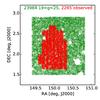 |
Fig. 1 Location on the sky of the galaxies observed with the VLT in this paper (red crosses). All COSMOS photometric redshift catalog detections are shown by green dots. |
2.4.1. Selection
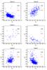 |
Fig. 2 Selection. u − b color vs. MB absolute magnitude for each selection with MB derived using the photometric redshift. The vertical bars show the mean 1σ error on the u and b bands for each selection. Class A objects are bright and blue. |
To completely fill the slit masks, we used six different selection schemes using the COSMOS catalog magnitudes (MAG AUTO not corrected for galactic extinction):
-
Class A: a griz +3.6 μm selection with 20 <g< 24 and i − z> (g − i)/2−0.1 and r − z> (i − mag3.6 μm)/3 and r − z> 0.8(g − i) + 0.1; these criteria select strong [Oii] emitters that are bright and blue. It was designed using the Cosmos Mock Catalog (Jouvel et al. 2009);
-
Class B: Herschel detected galaxies at 5σ (Lutz et al. 2011);
-
Class C: MIPS detected galaxies at 5σ (Le Floc’h et al. 2009);
-
Class D: ugr selection from Comparat et al. (2013b; 20 <g< 23.5, −0.5 <u − g< 1, −1 <g − r< 1, −0.5 <u − r< 0.5);
-
Class E: gri selection from Comparat et al. (2013b; −0.1 <g − r< 1.1, 0.8 <r − i< 1.4, 20.5 <i< 23.5);
-
Class F: a photometric redshift selection 1 <zphot< 1.7 and 20 <i< 24 to fill the remaining empty area of the masks.
Number of spectra observed.
Class A is the only sample on which one can perform a stand-alone statistical analysis. In fact, the slits placed on the other selections were constrained by the slits placed on the Class A targets; therefore, the obtained samples are not random subsamples of their parent selection. Table 1 describes the quantity of each class observed and the quality of the redshift obtained (see next section). The location of these samples in the u − b vs. MB absolute magnitude band is presented in Fig. 2. It shows that the Class A and C targets are bright and blue. A comparison of this selection with DEEP 2 observations (Mostek et al. 2013) demonstrates that Class A galaxies have stellar masses between 1010 M⊙ and 1011 M⊙ and an SFR> 101.2 M⊙ yr-1, and therefore possess strong [Oii] emission lines. The redshift efficiency for the Class A selection is 701/947 = 74.0% (692/947 = 73% have 0.6 <z< 1.7 and 552/947 = 58% have 1 <z< 1.7). The selections may seem complicated on first sight, though they were useful to minimize telescope time and measure a large number of [Oii] emitters. The Class A, D, and E selections try to mimic an absolute magnitude MB selection using optical bands. Class A is successful as it is 16% more efficient than the magnitude limited selection represented by Class F.
2.4.2. Data reduction, spectroscopic redshifts
The data processing pipeline performs an extraction of the spectrum that allows the estimation of the flux in the [Oii] emission line. This procedure has two steps.
-
1.
We apply the scripts and procedures from the ESO pipeline document2. We use fors_bias for the master bias creation, fors_calib for the master calibration creation, and fors_science to apply the calibrations and subtract the sky. Figures 8.2 and 8.3 from that document show an example of the data reduction cascade. We use the “unmapped” result obtained in the middle of the fors_science part of the reduction, and the matching frames containing the wavelength values. Both “average” and “minimum” combinations of the two frames are obtained on each mask.
-
2.
Emission lines are visually identified on both average and minimum reductions. The visual inspection is more efficient than an automated measurement because of the presence of cosmic ray residuals when combining the two exposures, and the strong variations of S/N across the two-dimensional spectra (both spatially and spectrally). A quality flag Q is assigned to each object: 4 (secure redshift identification), 3 (clear single line redshift identification), 2 (possible line, not 100% convincing), 1 (a rough estimate), 0 (strong defect preventing redshift measurement or line identification). We consider Q = 3 or 4 to be reliable redshifts (see Table 1). Given the wavelength coverage of the spectrum, there are only a few spectra with a single line that could be identified incorrectly. In those particular cases a quality Q = 2 was attributed.
As shown in Fig. 3 the redshifts measured for the galaxies in our study fill the gap between COSMOS 20 k and COSMOS Deep 4.5 k (Scoville et al. 2007b; Lilly et al. 2009). The highest redshift in our sample is zmax = 1.73. Classes B and C mainly contain galaxies at redshifts below z< 0.8.
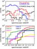 |
Fig. 3 Redshift distributions. Top: distribution of our sample (red solid line for Q = 3 or 4, dashed line for Q = 2) compared to previous spectroscopic programs on COSMOS: the COSMOS deep 4.5 k (black) and COSMOS 20 k (blue). Bottom: quality 3 or 4 redshift cumulative distributions for each class of target in our sample. |
There is a small overlap between the sample presented here and previous COSMOS spectroscopic samples; this allows us to compare the redshift of objects observed twice (the positions on the sky match within 0.1 arcsec). For the set of objects with Class A, 7 galaxies with Q = 3 and 26 with Q = 4 have a counterpart with a high quality flag. For the set of objects with Class ≠ A, 15 galaxies with Q = 3 and 21 with Q = 4 have a counterpart with a high quality flag. Among these matches, only two galaxies have a spectroscopic redshift that do not agree at the 10% level (dz> 0.1(1 + z)). After a second inspection of these redshifts we found that the redshifts we obtained are correct (see Fig. 4).
We also compared our spectroscopic redshifts to the photometric redshifts from Ilbert et al. (2009, 2013). We considered 1344 objects with both good spectroscopic redshift and photometric redshift. A total of 97.3% (1306) of the photometric redshifts are in agreement with the spectroscopic redshift within a 15% error, and 89.9% (1207) within a 5% error (see Fig. 5). The agreement is excellent.
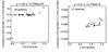 |
Fig. 4 Comparison between the spectroscopic redshift and the spectroscopic redshift from previous surveys. |
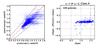 |
Fig. 5 Comparison between the spectroscopic redshift and photometric redshift. |
Finally, we fit the emission lines detected in the spectra using a simple Gaussian model for every line. Given the resolution of the spectrograph, one cannot detect the difference between the fit of a single Gaussian and the fit of a doublet for the [Oii] line. From this model we determined the emission line flux and the S/N of the detection. The [Oiii] line is detected in the redshift range 0.45 <z< 1.05 and [Oii] in the range 0.9 <z< 1.75. The S/N distribution is correlated to the quality flag of the redshifts (see Fig. 6). The exposure times were too short to measure the continuum, we therefore estimated the equivalent widths and the levels of the continuum using the broadband magnitude that contains the emission line. We used an extrapolation of the median aperture correction as a function of half light radius, based on the zCOSMOS corrections, to correct the fluxes from the aperture (see Fig. 7). Two examples of spectra are shown in Fig. 8.
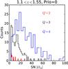 |
Fig. 6 S/N in the [Oii] lines for different redshift quality flags. The galaxies with Q = 3 or 4 are used to determine the LF. |
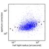 |
Fig. 7 Aperture correction factor vs. half light radius on Cosmos. The red stars represent the median correction for bins of half light radius. |
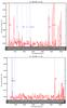 |
Fig. 8 Two spectra from the ESO VLT/FORS2 data set at redshift 0.92 and 1.6. The one-dimensional spectra (red) are on top of the two-dimensional spectra (shades of grey). |
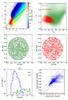 |
Fig. 9 Observations with the SDSS telescope based on the CFHTLS photometry. Top row, left: u − r vs. g − i colored according to the photometric redshift. The selection applied is in the dashed box. Right: color selection projected in the u − g vs. MG plane which shows our selection aims for the brightest and bluest objects. Middle row: RA, Dec in degrees (J2000). Left: g< 25 objects from the CFHT-LS W3 photometric redshift catalog. Right: targets observed spectroscopically. Bottom row, left: distribution of the redshifts observed. It is very efficient for selecting redshift 0.8 ELGs. Right: spectroscopic redshift and photometric redshift. The dashed lines represent the error contours at dz = 0.15(1 + z). The agreement is good. |
2.4.3. Galaxies with a flux [O ii] > 10-15 erg s-1 cm-2
There are three galaxies with [Oii] fluxes greater than 10-15 erg s-1 cm-2. Two are compact and have broad emission lines and are probably active galactic nuclei (AGNs). For the LF analysis, we removed the broad-line AGNs in order to be able to easily compare our results with other studies. The third galaxy appears disturbed and might be undergoing a merging process.
2.5. Data from SDSS-III/BOSS ELG ancillary program
Within the Sloan Digital Sky Survey III collaboration (SDSS; York et al. 2000; Eisenstein et al. 2011; Dawson et al. 2013), galaxies with strong emission lines (ELG) were observed in the redshift range 0.4 <z< 1.6 to test the target selection of emission line galaxies on two different photometric systems for the new SDSS-IV/eBOSS survey. These observations are part of the SDSS-III/BOSS ancillary program and are flagged “ELG” or “SEQUELS_ELG”. These spectra will be part of the SDSS data release 12 (DR12).
2.5.1. CFHT-LS ugri selection
During a first observation run, a total of 2292 fibers were allocated over 7.1 deg2 (the area of an SDSS-III plate). The ELG were observed for 2 h with the spectrograph (Smee et al. 2013) of the 2.5 m telescope located at Apache Point Observatory, New Mexico, USA, (Gunn et al. 2006). The targets were selected from the Canada-France-Hawaii Telescope Legacy Survey (CFHT-LS) Wide W3 field catalog with ugri bands. The data and cataloguing methods are described in Ilbert et al. (2006); Coupon et al. (2009), and the T0007 release document3.
The color selection used is  The selection function focuses on the brightest and bluest galaxy population (see Fig. 9). The selection provides 3784 targets, and we observed 2292 of them. The observations of this sample were obtained on the three SDSS plates numbered 6931, 6932, and 6933.
The reduction and the fit of the redshift is fully automated and performed by version v5_6_elg of the BOSS pipeline (Bolton et al. 2012). A total of 88.7% of the spectra observed have sufficient signal to be assigned a reliable redshift (see Table 2). Of this sample 82.3% are emission line galaxies (ELGs), 5.6% are quasars (QSOs), and 0.7% are stars. A total of 11.3% of the spectra have insufficient S/N to obtain a reliable spectroscopic redshift. The spectroscopic redshift distribution obtained is presented in Fig. 9. The photometric redshifts from T0007 on CFHT-LS W3 perform well. Of the 1609 galaxies with a photometric redshift and a good spectroscopic redshift, 92.3% (1486) are within a 15% error and 71.9% (1157) within a 5% error. The bluer objects tend to have larger uncertainties on the photometric redshifts. Improving CFHT-LS photometric redshifts for this population is of great interest, but is beyond the scope of this paper.
Observations on the CFHT-LS Wide 3 field.
2.5.2. SCUSS + SDSS ugri selection
A similar target selection was applied to a combination of SCUSS u-band survey4 (Xu Zhou et al., in prep.; Hu Zou et al., in prep.) and SDSS g,r,i photometry on a region of the sky of 25.7 deg2 around αJ2000 ~ 23° and δJ2000 ~ 20°. This observation run, with a total of 8099 fibers allocated, measured ELG spectra with exposure times of 1h30 and covered 25.7 deg2.
The color selection used is similar to the previous selection, but with a u magnitude limit instead of a g limit:  We also had a low priority ELG selection criterion (LOWP) to fill the remaining fibers. It is the same criterion stretched in magnitude and color to investigate the properties of the galaxies around the selection: [20 <u< 22.7 and −0.9 <u − r] and [u − r< 0.7·(g − i) + 0.2 or u − r< 0.7].
The BOSS pipeline was used to process the data and all the spectra were inspected to confirm the redshifts. The redshift distribution of this sample is shifted towards lower redshifts (see Fig. 10) with respect to the previous sample because of the shallower photometry (between 5 and 10 times shallower) from which the targets were drawn. This sample is complementary in terms of redshift and luminosity. Table 3 summarize the results of the observations.
We retained the split of the two ugri ELG samples because the parent photometry catalogs are very different.
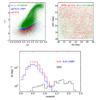 |
Fig. 10 Observations with SDSS telescope based on the SCUSS photometry. Top row, left panel: color selection applied to the SDSS + SCUSS photometry. Right panel: RA, Dec in degree (J2000). All the 20 <u< 23 objects (green) and the spectroscopic targets (red). Bottom: observed redshift distributions per square degree per Δz = 0.1 High priority ELG (red) are at slighter higher redshift than the low priority ELG (blue). This selection based on a shallower photometry than the CFHT-LS is not as efficient at selecting redshift 0.8 ELGs. |
SCUSS – SDSS-III/BOSS ELG observed as a function of spectral types.
2.5.3. Emission line flux measurement on BOSS spectra
The flux in the emission line derived from BOSS spectra were estimated using two different pipelines, the redshift pipeline (Bolton et al. 2012) and the Portsmouth pipeline5 (Thomas et al. 2013). These estimators produce consistent measurements. The BOSS spectra were observed with fiber spectroscopy, and objects are typically larger than the area covered by the fibers, which have a diameter of 2 arcsec. To correct this effect we computed the difference between the magnitude in a 2 arcsec aperture and the total model magnitude. Table 5 gives the magnitude used as a function of the redshift of the galaxy. If the difference is within the error of the total magnitude, we do not correct the measured [Oii] flux. If the difference is greater than the error, then we rescale the [Oii] flux, fmeasured, using the magnitudes m in which the [Oii] line is located. The correction used was 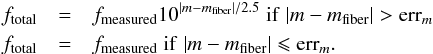 We cannot tell if the part of the galaxy located outside of the fiber actually emits more or less than the part measured within the fiber. The mean correction in flux is ~2.7; i.e., the fiber captured is on average ~40% of the total flux.
2.6. Galactic dust correction
We corrected the measured [Oii] fluxes from the extinction of our galaxy using the Calzetti et al. (1994) law fcorrected(λ) = fobserved100.4E(B − V), where E(B − V) is taken from the dust maps made by Schlegel et al. (1998).
2.7. Final sample
We combined the data samples previously described to measure the observed [Oii] LF in the redshift range 0.1 <z< 1.65. We set eight redshift bins of width ~1 Gyr.
We selected reliable redshifts that have well-defined photometry in two or three of the ugriz optical bands that we used for the weighting scheme (see next paragraph). Moreover, we requested a detection of the [Oii] lines with an S/N greater than 5. In total, we used around 20 000 spectra. The total amount of spectra provided by each survey as a function of redshift is given in Table 4.
This conjunction of surveys has a gap in redshift around redshift 0.45. We minimized the impact of this gap by shrinking the redshift bin to the minimum (0.4 <z< 0.5) and removing it from the analysis.
We tested the robustness of LF against the S/N limits between 3 and 10. We distinguished two regimes: for a S/N limit decreasing from 10 to 5, the uncertainty on the LF decreases and the luminosity limit decreases as the sample grows in size; for a S/N limit at 4 or 3, the number of detections increases, but the LF is not determined with greater precision. In fact, for such low significance detections the weights have a large uncertainty, which affects the LF. The most accurate results are obtained by using a S/N limit of 5.
We did not use the DEEP2 (Zhu et al. 2009; Newman et al. 2013), HETDEX (Ciardullo et al. 2013), and narrowband survey data from the Subaru Deep Field (Ly et al. 2007), from HiZELS (Sobral et al. 2012), or the UKIDSS Ultra Deep Survey field (Drake et al. 2013) because an [Oii] LF measurement had already been performed. Rather we compared their [Oii] LF measurements to ours.
Number of galaxies used in each redshift bin, by survey.
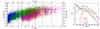 |
Fig. 11 Left panel: luminosity vs. redshift. In each redshift bin the horizontal black lines show the 5σ completeness limit of the data presented, except in the 0.4 <z< 0.5 where we show the high completeness limit (see Sect. 4.1 for details). Right panel: redshift distribution by survey, on the Cosmos field (purple), on the CFHT-LS W3 field (red), and on the SCUSS – SDSS field (green). |
3. [Oii] luminosity function
Based on the [Oii] catalog constructed in the previous section, we measured the [Oii] LF.
3.1. Weighting scheme
The weighting scheme relates the observed galaxies to their parent distribution; in this section, we describe a novel technique to compute the weights that allows different surveys to be combined.
3.1.1. Principle
In a dust-free theory, the [Oii] emitter population can be completely described by three parameters, the redshift, the continuum under the line (or the line equivalent width, EW), and the UV-slope that produced this emission. We denote with f the function that connects a point in the three-dimensional space (z, EW, UV-slope) to a unique [Oii] flux. Observationally, these three parameters correspond to the emission line flux, the magnitude containing the emission line, and the color preceding the emission line. In reality, the dust and orientation of each galaxy induces scatter in this parameter space introducing some scatter to the function f. The surroundings of each parameter of the relation should be considered so that f can still be used to relate the observed distribution to the parent distribution.
To implement this weighting scheme, we used the Megacam6 and SDSS photometric broadband ugriz filters (Fukugita et al. 1996; Gunn et al. 1998) systems (the SCUSS u filter is the same as the SDSS u filter) to assign a magnitude and a color as a function of the redshift of each galaxy. For example, in the Megacam system, a galaxy with a redshift in 0.1 <z< 0.461 will see its [Oii] line fall in the g band; we thus used the g magnitude and the u − g color to compare this galaxy to the complete population. For [Oii] redshifts in 0.461 <z< 0.561, we considered this zone as the overlap region between the g and the r filters. The boundaries are defined by the corresponding redshift of transition between the two bands zb broadened by 0.05, thus a transition of zb ± 0.05. In this bin, we used (g + r)/2 as the magnitude and u − g as the color. Table 5 and Fig. 12 present the colors and magnitudes assigned for the weighting. This process allows a consistent weighting scheme for the complete data set that has the same physical meaning when redshift varies.
Weighting scheme as a function of redshift for the [Oii] lines.
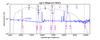 |
Fig. 12 Weighting scheme. Megacam transmission filters (gray lines) and the redshift bins (purple vertical lines) used to calculate the completeness weights. A rescaled spectrum of a typical emission line galaxy at redshift 0.6 is shown in blue. |
We computed the observed density deg-2 of galaxies with an S/N in the [Oii] emission line greater than 5, NobservedwithS/N [ OII ] > 5(zspec,m,c), as a function of spectroscopic redshift, magnitude m, and color c. This value is compared to the complete galaxy population Ntotal(zphot,m,c) to obtain a completeness weight, ![\begin{equation} W(z,m,c)=\frac{N_{\mathrm{observed \; with\; S/N} [{\rm O}_{\rm II}]\,>\,5}(z_{\rm spec},m,c)}{N_\mathrm{total}(z_{\rm phot},m,c)}\cdot \end{equation}](/articles/aa/full_html/2015/03/aa24767-14/aa24767-14-eq143.png) (2)To obtain the information on the complete galaxy population N_total(zphot,m,c), we used the photometric redshift catalogs from the CFHT-LS deep fields 1, 2, 3, 4 (WIRDS) (Ilbert et al. 2006, 2013; Bielby et al. 2012) and the Stripe 82 SDSS Coadd photometric redshift catalog (Annis et al. 2014; Reis et al. 2012) that span 3.19 deg2 and 275 deg2, respectively.
(2)To obtain the information on the complete galaxy population N_total(zphot,m,c), we used the photometric redshift catalogs from the CFHT-LS deep fields 1, 2, 3, 4 (WIRDS) (Ilbert et al. 2006, 2013; Bielby et al. 2012) and the Stripe 82 SDSS Coadd photometric redshift catalog (Annis et al. 2014; Reis et al. 2012) that span 3.19 deg2 and 275 deg2, respectively.
For redshifts z< 0.7, we used the number densities observed on the Stripe 82 SDSS Coadd. For redshifts above, we used the CFHT-LS deep photometric redshift catalog to obtain the best possible estimate of the parent density of galaxies (we note that it is not necessary to have the parent photometry and the observed data on the same location of the sky). We converted all the magnitudes to the CFHT Megacam system using the calibrations of Regnault et al. (2009) to have a consistent weighting scheme among the various surveys.
3.1.2. Implementation
To implement the weights properly and avoid edge effects caused by data binning, we adopted two three-dimensional trees7 (one for the data and one for the parent sample) containing the redshift, the magnitude, and the color normalized at their first and last deciles (D10 and D90); i.e., we remapped the three quantities so that the information is primarily contained in the interval 0–1
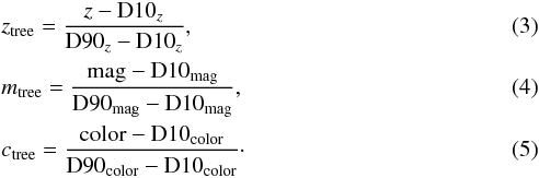 This transformation allows the estimation of distance between two points in the trees without being biased by the distribution of each quantity. In this manner the distance between two points i, j,
  (6)represents more equally the three axes: color, magnitude, and redshift. We computed the number of galaxies around each galaxy i in the observed sample tree and in the parent sample tree: N(Δi,obs< 0.15) and N(Δi,parent< 0.15). The ratio of the two numbers gives the individual weight for each observed galaxy.
Using the jackknife method, we tested the technique against different remapping schemes and tree distances and found the values mentioned above to be stable and reliable (see Appendix A for details). This method is more reliable than constructing color and magnitude bins, as binning can be very sensitive to the fine-tuning of each bin value, in particular at the edges of the distributions.
We estimated the sample variance uncertainty on N(Δi,obs< 0.15) and N(Δi,parent< 0.15) in two ways: the Poisson error and the Moster et al. (2011) “cosmic variance” estimator. In areas of high density of the three-dimensional tree, the Poisson error is negligible compared to the cosmic variance estimation. In regions of small densities, this relation is reversed. To avoid underestimating the error, we considered the sample variance error as the maximum of the two estimators.
The uncertainty on the weight (wErr) is computed by varying the position of the galaxy in both trees in all directions of the redshift, magnitude, and color space by its error in each dimension. This approach produces an upper and lower value for the weight. We note that the uncertainty in redshift is negligible compared to the error on the magnitude and color.
The final uncertainty on the weight is the combination of the sample variance and of the galaxy weight error. The weight error dominates on the edges of the redshift-magnitude-color space, where densities are sparse. The sample variance error dominates in the densest zones of the redshift-magnitude-color space.
This method is very similar to that of Zhu et al. (2009) where they express the probability of [Oii] being measured, denoted f, as a function of the object magnitude compared to the R-band cut, the B − R, R − I color cuts, and of the probability of measuring a good redshift with [Oii] in the spectra. From this probability they extract a completeness weight for each galaxy.
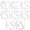 |
Fig. 13 Observed LF compared to previous surveys estimates (in their closest redshift bin). The number above each LF point gives the exact number of galaxies used. The arrows going downwards correspond to measurements with an error consistent with 0. The Schechter functions fits are shown as magenta dashes. The last panel shows the evolution of the [Oii] LF from redshift 0.17 to 1.44 using the fits. The trend is that with increasing redshift there are increasing numbers of bright [Oii] emitters and the faint end slope gets steeper. |
3.2. Observed luminosity function
We define the luminosity in the [Oii] lines by ![\begin{equation} L_{\left[\mathrm{O\textrm{\textsc{ii}}}\right]\,} \; \left[{\rm erg\, s}^{-1}\right]=4 \pi \; \left( {\rm flux \; \left[\mathrm{O\textrm{\textsc{ii}}}\right] \; \left[{\rm erg\, s^{-1} \,cm}^{-2}\right] } \right) \left[ \frac{{\rm d}_{L(z)}}{[{\rm cm}]} \right]^2, \end{equation}](/articles/aa/full_html/2015/03/aa24767-14/aa24767-14-eq155.png) (7)where dL is the luminosity distance in cm expressed as
(7)where dL is the luminosity distance in cm expressed as 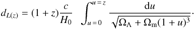 (8)The completeness limit is given by the completeness limit of the data sample with the highest sensitivity.
Fits on the LF.
We used the jackknife technique to estimate sample variance on the LF. We split the sample into ten equal subsamples and remeasured the LF on the subsamples. The standard deviation from the ten estimations is our adopted sample variance error. The LF measurements are shown in Fig. 13. The error bars contain the error from the weight (wErr) and the sample variance error computed with jackknife.
Thanks to the combination of the GAMA survey and the low redshift ELG observed in SEQUELS, we were able to estimate the [Oii] LF at low redshift (z< 0.4) and in particular accurately measure its bright end. The combined fit with the HETDEX measurement gives a good estimation of the parameters of the Schechter model.
In the redshift bin 0.4 <z< 0.5, the completeness from GAMA drops and the other spectroscopic samples were selected to be at higher redshift. Therefore, it is difficult to derive a clean LF in this bin and we excluded it from the analysis.
In the three redshift bins within 0.5 <z< 1.07, we were able to compare the Drake et al. (2013) measurement in the first bin and the Zhu et al. (2009) measurements in the following two bins. In the first bin the Drake et al. (2013) measurement is at slightly lower redshift (0.53 compared to 0.6) and given the quick evolution of the LF at this epoch the discrepancy found is reasonable. In the following two bins, given that the DEEP2 measurements are at a slightly higher redshift, they are brighter. In these bins, a Schechter (1976) model fits the LF well. In particular, the faint completeness limit allows the faint end slope of the LF to be fitted accurately.
In the last two redshift bins, 1.07 <z< 1.65, the LF measurement is in very good agreement with the previous DEEP2 measurements, although our data sets are limited to the bright end that only corresponds to a part of the SFR density in these bins. To constrain the faint end slope of the Schechter fits in these bins, we use the measurements from Sobral et al. (2012); Drake et al. (2013). We note that these measurement are in very good agreement in the overlapping region.
Our measurement clearly shows the evolution of the bright end of the [Oii] LF: as redshift increases from 0.165 to 1.44, there are more luminous [Oii] emitters. The last panel of Fig. 13 show the evolution using the fits. Thanks to the combination with the measurements of the faint end by Sobral et al. (2012); Drake et al. (2013) in the last two redshift bins and by Gilbank et al. (2010); Ciardullo et al. (2013) in the first two redshift bins, we can also notice the steepening of the faint end slope from redshift 0.165 to redshift 1.44.
We computed the integrated luminosity density directly without using any fits (see Table 6). Then using the latest [Oii] SFR calibration from Moustakas et al. (2006) we converted this luminosity density into a SFR density: ![\begin{equation} \frac{\rho {\it SFR}_{\left[\mathrm{O\textrm{\textsc{ii}}}\right]}}{M_\odot \; {\rm yr^{-1}\; Mpc}^{-3}}=\frac{2.18\times 10^{-41} \mathcal{L}(\left[\mathrm{O\textrm{\textsc{ii}}}\right])} {[{\rm erg \; s^{-1} \; Mpc^{-3}}]}\cdot \label{sfr:kennicutt} \end{equation}](/articles/aa/full_html/2015/03/aa24767-14/aa24767-14-eq199.png) (9)Given that Moustakas et al. (2006) demonstrated that the [Oii] SFR is subject to uncertainties of ~0.4 dex (a factor of 2.5), the numbers in Table 6 should be considered with care. We note that this result is not corrected for the extinction. Given that we integrate directly on the measurement and not on the fit, these values can only be considered as lower limits to the total SFR density.
(9)Given that Moustakas et al. (2006) demonstrated that the [Oii] SFR is subject to uncertainties of ~0.4 dex (a factor of 2.5), the numbers in Table 6 should be considered with care. We note that this result is not corrected for the extinction. Given that we integrate directly on the measurement and not on the fit, these values can only be considered as lower limits to the total SFR density.
The overall trend, which is independent of any fits, is the increase of the integrated luminosity density ℒ([Oii])(z = 0.165) ~ 39 to ℒ([Oii])(z = 1.44) ~ 40; this confirms that there are more [Oii] emissions at z> 1 than at z< 1.
3.3. Functional form of the luminosity function
The number density of galaxies in the luminosity range L + dL, denoted Φ(L)dL, is usually fitted with a Schechter (1976) function of the form 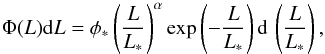 (10)where the fitted parameters are α the faint end slope, L∗ [erg s-1] the characteristic Schechter luminosity, and φ∗ [Mpc-3] the density of galaxies with L>L∗. The parameters fitted are usually highly correlated. Gallego et al. (2002) found a faint end slope of −1.2 ± 0.2 with a Schechter model for ELGs in the local Universe. Gilbank et al. (2010) remeasured the [Oii] LF in the local Universe, but found that a model with a double power-law and a faint end slope of −1.6 was a better representation of the data. Zhu et al. (2009) also found that a double power law was a better description of the [Oii] LF.
Our new LF measurement demonstrates that the Schechter model fits the data well. Based on the Schechter fits, we measured the evolution over 8 Gyr of log L∗ from 42.41 at redshift 1.44 to 41.18 at redshift 0.165.
The parameter α is not well constrained in the literature; with this measurement, we now have a better insight on its value and evolution. Beyond redshift z> 1.1, the completeness limit of our sample is too bright to constrain α, but combining with narrowband estimates of the LF enables the fit of α. We measure the flattening of the LF from redshift 1.44 to redshift 0.165 (see Table 6).
The results of the fits are summarized in Table 6 and are shown in Fig. 13.
3.4. [OII] flux limited redshift surveys, baryonic acoustic oscillation, and emission line galaxy target selection
Future large spectroscopic surveys that aim for a precise measurement of the baryonic acoustic oscillations (BAO) in the power spectrum of galaxies in the redshift range 0.7 <z< 1.6, such as DESI8 or eBOSS9, can be designed following three constraints.
First, the measured power spectrum of the tracers surveyed must overcome the shot noise, which requires a high density of tracers. We can distinguish two regimes of selection below redshift z< 1.1, and above. At z = 0.7, the power spectrum of the dark matter predicted by the Code for Anisotropies in the Microwave Background, CAMB (Lewis et al. 2000), is P(k = 0.063 h Mpc-1) = 9.5 × 10³h3 Mpc-3, thus a density of  Mpc-3 is sufficient to overcome the shot noise by a factor three (Kaiser 1986). At z = 1.1, P(k = 0.063 h Mpc-1) = 7. × 103h3 Mpc-3, and the density required is 4.2 × 10⁻⁴ Mpc-3. In the redshift range 0.7 <z< 1.1, the massive M> 1011 M⊙ galaxy population consists of a mix of star-forming and quiescent galaxies, whose number density is ~2 × 10⁻³ Mpc-3 (Ilbert et al. 2013). The galaxy densities to overcome shot noise are therefore reachable either with the quiescent or the star-forming galaxies. At z = 1.6, P(0.063 h Mpc-1) = 5. × 103h3 Mpc-3, the density required is 6 × 10⁻⁴ Mpc-3. From the galaxy evolution point of view, a significant change occurs in the redshift range 1.1 <z< 1.6: the massive end (M> 1011 M⊙) of the mass function becomes dominated by star-forming galaxies. The density of massive star-forming galaxies is around ~10-3 Mpc-3, whereas the density of massive quiescent galaxies drops from 6 × 10⁻⁴ Mpc-3 at z = 1.1 to 10-4 Mpc-3 at z = 1.6. Therefore, above redshift z> 1.1 the density of massive quiescent galaxies decreases too rapidly to overcome the shot noise in the power spectrum of galaxies. However, the density of massive star-forming galaxies in the redshift range 0.7 <z< 1.6 is sufficient to sample the BAO: this tracer covers this redshift range consistently. Therefore, to overcome shot noise and measure the BAO in the power spectrum of galaxies, one must target star-forming galaxies.
Second, because of the large load of required data in BAO experiments, accurate spectroscopic redshifts must be acquired in an effective manner. Star-forming galaxies have strong emission lines in their spectrum, and are therefore good candidates. Comparat et al. (2013b) demonstrated that one can select efficient star-forming galaxies to sample the BAO to redshift z = 1.2. The [Oii] LF measurement presented here extends this measurement to redshift 1.65 and provides insight on the galaxy population considered by future BAO studies compared to the global galaxy population.
Third, there is the need to survey massive galaxies that are well correlated to the whole matter field (luminous and dark) in order to obtain the highest possible S/N in their power spectrum. Comparat et al. (2013a) demonstrated that the color-selected galaxies for BAO have a relatively high galaxy bias b ~ 1.8, and their luminous matter – dark matter cross-correlation coefficient measured using weak-lensing is consistent with 1, but we do not consider this point in this article. Therefore, one needs to select the most luminous galaxies of the redshift range to maximize the galaxy bias.
To detect the BAO at redshifts above z> 0.7, with optical spectrographs, an [Oii] flux-limited sample is therefore the best way to cover the entire redshift range in a minimum amount of telescope time with a dense enough galaxy population. This selection is equivalent to making a SFR selection plus a dust selection (selecting galaxies with the least amount of dust) so that lines emitted are not obscured. This sample will neither be a mass-limited sample nor a SFR-limited sample.
Based on the catalog gathered to compute the LF, we can derive relations between the [Oii] flux observed and magnitudes to help the planning of theses surveys, in particular the target selection algorithms. We investigate the eventual correlations between the observed [Oii] fluxes and the ugriz broadband magnitude (in the CFHT Megacam system). We set two redshift ranges:
-
0.7 <z< 1.1 corresponding to eBOSS-ELG and where the [Oii] data is complete to a luminosity of 1041 erg s-1, which corresponds to a flux 2.3 × 10⁻¹⁷ erg s-1 cm-2 at redshift 0.9.
-
1.1 <z< 1.6 corresponding to DESi-ELG and where the [Oii] data is complete to a luminosity of 1042 erg s-1, which corresponds to a flux 8.2 × 10⁻¹⁷ erg s-1 cm-2 at redshift 1.3.
The magnitude that correlates best with the [Oii] flux is the g band in the redshift range 0.7 <z< 1.1 and the r band in the range 1.1 <z< 1.6 (see Fig. 15). These bands should thus be used to construct an [Oii] flux limited sample in the most efficient way. The correlation in the higher redshift bin might be biased because below the flux completeness limit the data is not representative of the complete population: u or g band could also be used for targeting at redshift 1.1 <z< 1.6.
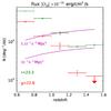 |
Fig. 14 Redshift distribution per square degree of galaxies with [Oii] flux greater than 10-16 erg s-1 cm-2 and magnitude g brighter than r< 23.3 (green) and g< 22.8 (red) compared to constant density of 10-3 and 3 × 10⁻⁴h3 Mpc-3 (purple). |
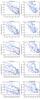 |
Fig. 15 Correlations between the broadband magnitudes and the [Oii] flux. The contours represent the density of galaxies predicted by the weighted data (from dark blue to brown 10, 50, 100, 200, 500 galaxy deg-2). The g band correlates best in the redshift range 0.7 <z< 1.1. The r magnitude correlates best in the range 1.3 <z< 1.6. The fluxes corresponding to a luminosity of 1041 and 1042 erg s-1 and the mean redshift (0.9 and 1.3) are represented by dashed blue lines. |
We project the LF densities as a function of redshift to derive the brightest g and r limiting magnitude that will provide a sufficient density of the brightest [Oii] emitters (a flux limit of 10-16 erg s-1 cm-2) to sample the BAO. We find that a survey with magnitude limit of g< 22.8 can target a tracer density greater than 10-4 galaxies h3 Mpc-3 to z ~ 1.2 (e.g., eBOSS). A survey with magnitude limit of r< 23.3 can target a tracer density greater than 10-4 galaxies h3 Mpc-3 to z ~ 1.6 (e.g., DESI; see Fig. 14). Further color selection is needed to sculpt the redshift distribution, in particular to remove lower redshift galaxies. We do not investigate color selections to separate [Oii] emitters in a given redshift range from the bulk of the galaxy populations at unwanted redshifts here. These color selections are dependent on the photometric survey used and should be discussed in each survey paper.
Comparing the magnitude – [Oii] fluxes correlations and their densities with the current observational plans of surveys such as DESI or eBOSS broadly confirms their feasibility.
[OII] and stellar mass
In addition to the relation between [Oii] flux and observed magnitudes, in order to plan future surveys and run N-body simulations with the adequate resolution, the stellar mass of the targeted ELG is of interest. We use the stellar mass catalog from (Ilbert et al. 2013) to estimate the average stellar mass of the samples mentioned above. The mean stellar mass of the eBOSS-ELG sample is 1010.2 ± 0.3 M⊙ and the mean stellar mass for the DESI-ELG sample is 109.9 ± 0.2 M⊙. This estimate confirms that ELG samples are not mass-limited sample (complete in mass). This confirms that an [Oii] -selected sample is likely to miss the dusty and star-forming galaxy population (Hayashi et al. 2013) that lies in the massive end of the galaxy population (Garn & Best 2010).
3.5. [OII] and star formation rate
The oxygen [Oii] emission line is also a SFR indicator that is measurable in the optical wavelengths for galaxies with redshift 0 <z< 1.7, thanks to its strength and its blue rest-frame location (Kewley et al. 2004), although the SFR-[Oii] relation is not as direct as SFR-Hα. The oxygen emission lines are not directly coupled to the ionizing continuum emitted by stars, but are sensitive to metal abundance, excitation, stellar mass, and dust-attenuation (e.g., Moustakas et al. 2006). The [Oii] lines are therefore more weakly correlated to the SFR owing to a number of degeneracies (Garn & Best 2010). In the past, the [Oii] LFs were derived and related to the SFR by Gallego et al. (2002); Ly et al. (2007); Argence & Lamareille (2009); Zhu et al. (2009); Gilbank et al. (2010). In order to derive a clean estimation of the SFR density sampled, we would need to recalibrate the [Oii] SFR relation in each redshift bin using a sample containing the [Oii] fluxes, the FUV, and IR luminosities. We leave this work for a future study.
4. Comparison to semi-analytical models
In this section we compare our observations to the predictions from two semi-analytical models, galform (Cole et al. 2000) and sag (Orsi et al. 2014), which are based on a ΛCDM universe with WMAP7 cosmology (Komatsu et al. 2011). In order to make the comparison with these models, we recomputed the observed LF for a WMAP7 cosmology.
Semi-analytical models use simple, physically motivated recipes and rules to follow the fate of baryons in a universe in which structure grows hierarchically through gravitational instability (see Baugh 2006; Benson 2010, for an overview of hierarchical galaxy formation models).
Here, we compare our observations to predictions from both the Gonzalez-Perez et al. (2014) flavor of the galform model (hereafter GP14) and the Orsi et al. (2014) flavor of the sag model (hereafter OR14). Both models follow the physical processes that shape the formation and evolution of galaxies, including
-
1.
the collapse and merging of dark matter haloes;
-
2.
the shock-heating and radiative cooling of gas inside dark matter haloes, leading to the formation of galaxy discs;
-
3.
star formation bursts that can be triggered by either mergers or disk instabilities;
-
4.
quiescent star formation in galaxy discs which in the OR14 model is assumed to be proportional to the total amount of cold gas, while in the GP14 model it takes into account both the atomic and molecular components of the gas (Lagos et al. 2011);
-
5.
the growth of super massive black holes in galaxies;
-
6.
feedback from supernovae, from AGNs and from photoionization of the intergalactic medium;
-
7.
chemical enrichment of the stars and gas;
-
8.
galaxy mergers driven by dynamical friction within common dark matter haloes, leading to the formation of stellar spheroids.
The end product of the calculations is a prediction for the number and properties of galaxies that reside within dark matter haloes of different masses.
Although both the GP14 and OR14 models assume the same cosmology, they use different N-body simulations to generate their respective dark matter halo merger trees. The GP14 model used the MS-W7 N-body simulation (Lacey et al., in prep.), with a simulation box of 500 h-1 Mpc side. The OR14 model was run using an N-body simulation of volume (150 h-1 Mpc)3. This volume is too small to adequately model the properties of the brightest observed galaxies. Tests using the GP14 model showed that a simulation box with sides of at least 280 h-1 Mpc is required to study the bright end of the [Oii] LF.
The free parameters in the GP14 model were chosen to reproduce the observed LFs at z = 0 in both b and K bands and to give a reasonable evolution of the rest-frame UV and V LFs. To calibrate their free parameters, the OR14 model used the z = 0 LFs, but also the z = 1 UV LF and SN Ia rates (Ruiz et al. 2013).
Both the GP14 and OR14 models reproduce the evolution of the HαLF reasonably well (Lagos et al. 2014; Orsi et al. 2014). The Hαis a recombination line and thus, its unattenuated luminosity is directly proportional to the Lyman continuum, which is a direct prediction of the semi-analytical models. Below we briefly describe how the emission lines are calculated in both models.
4.1. The GALFORM model
In the galform model the ratio between the [Oii] and the Lyman continuum is calculated using the Hiiregion models by Stasińska (1990). The galform model uses by default eight Hiiregion models spanning a range of metallicities, but with the same uniform density of 10 hydrogen particles per cm-3 and one ionizing star in the center of the region with an effective temperature of 45 000 K. The ionizing parameter10 of these Hiiregion models is around 10-3, with exact values depending on their metallicity in a nontrivial way. These ionizing parameters are typical within the grid of Hiiregions provided by Stasińska (1990).
In this way, the galform model is assuming a nearly invariant ionization parameter. Such an assumption, although reasonable for recombination lines, is likely too simplistic for other emission lines such as the [Oii] line (e.g., Sanchez et al. 2015).
4.2. The SAG model
Orsi et al. (2014) combined the sag semi-analytical model with a photo-ionization code to predict emission line strengths originated in Hiiregions with different ionization parameters. In order to do this, the model assumes an ionization parameter that depends on the cold gas metallicity of the galaxy. This dependency is suggested by a number of observational studies (e.g., Shim & Chary 2013; Sanchez et al. 2015).
The dependency of the ionization parameter on metallicity introduced two new free parameters in the OR14 model, an exponent and a normalization, that were chosen in order to reproduce the observed BPT diagram and the [Oii] and [Oiii] LF at different redshifts obtained by narrowband surveys.
4.3. The predicted [OII] luminosity function
Our observed [Oii] LF at z = 0.6, 0.95, 1.2, and 1.44 are compared with the predictions from both the GP14 and the OR14 models in Fig. 16. It is important to stress that the GP14 model was not calibrated to reproduce any observed [Oii] LF and that the OR14 was calibrated by attempting to reproduce the [Oii] LFs of narrowband observations, which do not suffer from the same selection effects as the ones derived here.
The OR14 model predicts an [Oii] LF with a bright end slope that agrees with our observations at all redshifts. As shown in Fig. 16, the [Oii] LF predicted by the OR14 model at z = 1.44 is in excellent agreement with our observations and with other observations. However, at lower redshifts this model overpredicts the density of faint [Oii] emitters. Figure 16 shows that the predictions of the OR14 are affected by the modeling of dust.
Figure 16 shows that the observed [Oii] LFs at z ≃ 1.2 is reasonably reproduced by the prediction from the GP14 model. The GP14 model underpredicts the observed [Oii] LF at z = 1.44, except for the brightest bins, which is dominated by the emission of central galaxies. The predicted [Oii] LF by the galform model is sensitive to the assumed ionization parameter. Using extreme values from the Stasińska (1990) grid of Hiiregions, we obtain predicted [Oii] LFs bracketing those shown in Fig. 16. The default characteristics of the Hiiregion model assumed in the galform model might not be adequate at the higher redshifts z = 1.44. For the two highest redshift bins shown in Fig. 16, the observations are actually closer to the predicted LF without dust attenuation, though it is unlikely for these galaxies to be dust free. In particular, if we take into account that the dust extinction applied to the [Oii] line is the same as experienced by the continuum at that wavelength, the line could actually be more attenuated than predicted here. The main uncertainty for the Hαline is the dust attenuation (see Gonzalez-Perez et al. 2013, for a detailed description of the dust treatment in the models).
Figure 16 also shows the [Oii] LF predicted by the GP14 model imposing a cut in magnitude similar to that done observationally. Compared with the model predictions, we expect our observations to be complete at the faintest end of the LF. A detailed exploration of the source of the discrepancy between our observations and the predictions from both models is beyond the scope of this paper.
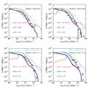 |
Fig. 16 Our observed LF (black symbols) compared to the predictions from the GP14 (solid blue lines) and the OR14 model (solid green lines). The solid red lines show the predictions from the GP14 model when an extra cut in magnitude is included, as indicated in each legend. The corresponding predictions without including the dust attenuation are shown as dashed lines of the corresponding color. We have also included for comparison the observational data from Drake et al. (2013) as cyan symbols. |
5. Conclusion
In this work we have measured the [Oii] LF every gigayear in the redshift range 0.1 <z< 1.65 with unprecedented depth and accuracy. This has allowed us to witness the evolution of its bright end: we measure the decrease of log L∗ from 42.4 erg/s at redshift 1.44 to 41.2 at redshift 0.165. Moreover, by combining our measurements with the fainter ones by Sobral et al. (2012); Drake et al. (2013) and Gilbank et al. (2010); Ciardullo et al. (2013), we measure the faint end slope flattening from redshift 1.44 to 0.165.
Such a measurement has been made possible by combining observations in a novel way from the FORS2 instrument at VLT on the COSMOS field (released along with the paper), the SDSS-III/BOSS spectrograph ELG ancillary programs, and with public flux calibrated spectroscopy of [Oii] emitters. Indeed, we created a new weighting scheme that robustly combines different data sets for observations that provide the measurement of the fluxes in the lines, the corresponding aperture correction, and the parent photometry.
The measurement of the bright end of the LF demonstrates the feasibility of eBOSS and DESi emission line galaxy target selection; i.e., we have shown here that the density of galaxies with emission line fluxes >10-16 erg s-1 cm-2 is sufficient to sample the BAO to redshift 1.6.
We have compared our observed [Oii] LF to predictions from two state-of-the-art semi-analytical models, and find a good agreement. This comparison is encouraging for the viability of producing realistic mock catalogs of [Oii] flux limited surveys, though more work is needed to understand the discrepancies found.
Online material
Appendix A: Weights
This appendix describes the details of the weighting scheme.
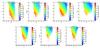 |
Fig. A.1 Predictions from the CMC for magnitude vs. color (in the CFHT system) and observed [Oii] luminosity for the CFHT magnitude redshift bins described in Table 5 and Fig. 12. |
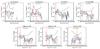 |
Fig. A.2 LF(d)/LF(0.15) ratio for d = 0.11, 0.12, 0.13, 0.14, 0.16, 0.17, 0.18 divided by the LF determined with 0.15. The vertical red line is the luminosity completeness limit. The error on the LF is shown by black dashes. The LFs with radius 0.14 and 0.16 stay well within the uncertainty on the LF, while larger or smaller radii approach the limit of the uncertainty of the LF. |
The theoretical relation between the magnitude containing [Oii], the color before this magnitude, redshift, and the [Oii] luminosity is shown using the Cosmo Mock Catalog (Jouvel et al. 2009) in Fig. A.1. This representation does not take into account the dust present in the galaxies that will induce scatter in this figure. For a constant magnitude, the most luminous galaxies have a blue color. This simulation is based on the Kennicutt laws, an extrapolation of the DEEP2 [Oii] LF, and ignores dust effects. Therefore, this test cannot be used at face value, not even to determine the completeness limit of our sample. This analysis provides an idea on the relation between the magnitude limit and the luminosity completeness limit we can reach with a sample.
In the text, we quote as best value for the tree search a distance of 0.15. This distance corresponds to a maximum distance in each direction of 0.088, and constrains the search for neighbors within about ~±0.5 mag around the magnitude, about ~±0.25 mag around the colors, and about ~±0.15 around the redshift. These values approximately correspond to the area a given galaxy population occupies (see Fig. A.1).
We tested the LF estimation for different distance values and found that a limit at 0.15 ± 0.01 was stable and variations in the measurement of the LF would be smaller than the uncertainty on the LF. Figure A.2 shows the variation in the LF compared to the LF estimate using the tree search distance 0.15. For tree searches that are too wide (>0.17) the weighting scheme begins to fail; i.e., the LF is inconsistent at 1σ with the fiducial LF. For tree searches that are too narrow (<0.13), the weights become inaccurate, the weight error increases, and the LF is less accurate.
The ionizing parameter is defined here as a dimensionless quantity equal to the ionizing photon flux per unit area per hydrogen density, normalized by the speed of light (see Stasińska 1990).
Acknowledgments
We thank Alvaro Orsi for sending us his model predictions and for the useful discussion. We thank the referee for constructive and insightful comments on the draft. J.C. acknowledges financial support from MINECO (Spain) under project number AYA2012-31101. J.R. acknowledges support from the ERC starting grant CALENDS. J.P.K. and T.D. acknowledge support from the LIDA ERC advanced grant. Funding for SDSS-III has been provided by the Alfred P. Sloan Foundation, the Participating Institutions, the National Science Foundation, and the U.S. Department of Energy Office of Science. The SDSS-III web site is http://www.sdss3.org. SDSS-III is managed by the Astrophysical Research Consortium for the Participating Institutions of the SDSS-III Collaboration including the University of Arizona, the Brazilian Participation Group, Brookhaven National Laboratory, University of Cambridge, Carnegie Mellon University, University of Florida, the French Participation Group, the German Participation Group, Harvard University, the Instituto de Astrofisica de Canarias, the Michigan State/Notre Dame/JINA Participation Group, Johns Hopkins University, Lawrence Berkeley National Laboratory, Max Planck Institute for Astrophysics, Max Planck Institute for Extraterrestrial Physics, New Mexico State University, New York University, Ohio State University, Pennsylvania State University, University of Portsmouth, Princeton University, the Spanish Participation Group, University of Tokyo, University of Utah, Vanderbilt University, University of Virginia, University of Washington, and Yale University. The BOSS French Participation Group is supported by Agence Nationale de la Recherche under grant ANR-08-BLAN-0222. This work used the DiRAC Data Centric system at Durham University, operated by the Institute for Computational Cosmology on behalf of the STFC DiRAC HPC Facility (www.dirac.ac.uk). This equipment was funded by BIS National E-infrastructure capital grant ST/K00042X/1, STFC capital grant ST/H008519/1, and STFC DiRAC Operations grant ST/K003267/1 and Durham University. DiRAC is part of the National E-Infrastructure. V.G.P. acknowledges support from a European Research Council Starting Grant (DEGAS-259586) and the Science and Technology Facilities Council (grant number ST/F001166/1). Based on observations obtained with MegaPrime/Megacam, a joint project of CFHT and CEA/DAPNIA, at the Canada-France-Hawaii Telescope (CFHT) which is operated by the National Research Council (NRC) of Canada, the Institut National des Science de l’Univers of the Centre National de la Recherche Scientifique (CNRS) of France, and the University of Hawaii. The SCUSS is funded by the Main Direction Program of Knowledge Innovation of Chinese Academy of Sciences (No. KJCX2-EW-T06). It is also an international cooperative project between National Astronomical Observatories, Chinese Academy of Sciences and Steward Observatory, University of Arizona, USA. Technical supports and observational assistances of the Bok telescope are provided by Steward Observatory. The project is managed by the National Astronomical Observatory of China and Shanghai Astronomical Observatory. GAMA is a joint European-Australasian project based around a spectroscopic campaign using the Anglo-Australian Telescope. The GAMA input catalog is based on data taken from the Sloan Digital Sky Survey and the UKIRT Infrared Deep Sky Survey. Complementary imaging of the GAMA regions is being obtained by a number of independent survey programs including GALEX MIS, VST KiDS, VISTA VIKING, WISE, Herschel-ATLAS, GMRT and ASKAP providing UV to radio coverage. GAMA is funded by the STFC (UK), the ARC (Australia), the AAO, and the participating institutions. The GAMA website is http://www.gama-survey.org.
References
- Annis, J., Soares-Santos, M., Strauss, M. A., et al. 2014, ApJ, 794, 120 [NASA ADS] [CrossRef] [Google Scholar]
- Argence, B., & Lamareille, F. 2009, A&A, 495, 759 [NASA ADS] [CrossRef] [EDP Sciences] [Google Scholar]
- Baldry, I. K., Alpaslan, M., Bauer, A. E., et al. 2014, MNRAS, 441, 2440 [NASA ADS] [CrossRef] [Google Scholar]
- Baugh, C. M. 2006, Rep. Prog. Phys., 69, 3101 [NASA ADS] [CrossRef] [Google Scholar]
- Benson, A. J. 2010, Phys. Rep., 495, 33 [NASA ADS] [CrossRef] [Google Scholar]
- Bielby, R., Hudelot, P., McCracken, H. J., et al. 2012, A&A, 545, A23 [NASA ADS] [CrossRef] [EDP Sciences] [Google Scholar]
- Bolton, A. S., Schlegel, D. J., Aubourg, É., et al. 2012, AJ, 144, 144 [NASA ADS] [CrossRef] [Google Scholar]
- Calzetti, D., Kinney, A. L., & Storchi-Bergmann, T. 1994, ApJ, 429, 582 [NASA ADS] [CrossRef] [Google Scholar]
- Capak, P., Aussel, H., Ajiki, M., et al. 2007, ApJS, 172, 99 [NASA ADS] [CrossRef] [Google Scholar]
- Ciardullo, R., Gronwall, C., Adams, J. J., et al. 2013, ApJ, 769, 83 [NASA ADS] [CrossRef] [Google Scholar]
- Cole, S., Lacey, C. G., Baugh, C. M., & Frenk, C. S. 2000, MNRAS, 319, 168 [NASA ADS] [CrossRef] [Google Scholar]
- Comparat, J., Jullo, E., Kneib, J.-P., et al. 2013a, MNRAS, 433, 1146 [NASA ADS] [CrossRef] [Google Scholar]
- Comparat, J., Kneib, J.-P., Escoffier, S., et al. 2013b, MNRAS, 428, 1498 [NASA ADS] [CrossRef] [Google Scholar]
- Coupon, J., Ilbert, O., Kilbinger, M., et al. 2009, A&A, 500, 981 [NASA ADS] [CrossRef] [EDP Sciences] [Google Scholar]
- Dawson, K. S., Schlegel, D. J., Ahn, C. P., et al. 2013, AJ, 145, 10 [Google Scholar]
- Drake, A. B., Simpson, C., Collins, C. A., et al. 2013, MNRAS, 433, 796 [NASA ADS] [CrossRef] [Google Scholar]
- Driver, S. P., Hill, D. T., Kelvin, L. S., et al. 2011, MNRAS, 413, 971 [NASA ADS] [CrossRef] [Google Scholar]
- Eisenstein, D. J., Weinberg, D. H., Agol, E., et al. 2011, AJ, 142, 72 [Google Scholar]
- Fukugita, M., Ichikawa, T., Gunn, J. E., et al. 1996, AJ, 111, 1748 [NASA ADS] [CrossRef] [Google Scholar]
- Gallego, J., García-Dabó, C. E., Zamorano, J., Aragón-Salamanca, A., & Rego, M. 2002, ApJ, 570, L1 [NASA ADS] [CrossRef] [Google Scholar]
- Garn, T., & Best, P. N. 2010, MNRAS, 409, 421 [NASA ADS] [CrossRef] [Google Scholar]
- Gilbank, D. G., Baldry, I. K., Balogh, M. L., Glazebrook, K., & Bower, R. G. 2010, MNRAS, 405, 2594 [NASA ADS] [Google Scholar]
- Gonzalez-Perez, V., Lacey, C. G., Baugh, C. M., Frenk, C. S., & Wilkins, S. M. 2013, MNRAS, 429, 1609 [NASA ADS] [CrossRef] [Google Scholar]
- Gonzalez-Perez, V., Lacey, C. G., Baugh, C. M., et al. 2014, MNRAS, 439, 264 [NASA ADS] [CrossRef] [Google Scholar]
- Gunawardhana, M. L. P., Hopkins, A. M., Bland-Hawthorn, J., et al. 2013, MNRAS, 433, 2764 [NASA ADS] [CrossRef] [Google Scholar]
- Gunn, J. E., Carr, M., Rockosi, C., et al. 1998, AJ, 116, 3040 [NASA ADS] [CrossRef] [Google Scholar]
- Gunn, J. E., Siegmund, W. A., Mannery, E. J., et al. 2006, AJ, 131, 2332 [NASA ADS] [CrossRef] [Google Scholar]
- Hayashi, M., Sobral, D., Best, P. N., Smail, I., & Kodama, T. 2013, MNRAS, 430, 1042 [NASA ADS] [CrossRef] [Google Scholar]
- Hopkins, A. M., Driver, S. P., Brough, S., et al. 2013, MNRAS, 430, 2047 [NASA ADS] [CrossRef] [Google Scholar]
- Ilbert, O., Arnouts, S., McCracken, H. J., et al. 2006, A&A, 457, 841 [NASA ADS] [CrossRef] [EDP Sciences] [Google Scholar]
- Ilbert, O., Capak, P., Salvato, M., et al. 2009, ApJ, 690, 1236 [NASA ADS] [CrossRef] [Google Scholar]
- Ilbert, O., McCracken, H. J., Le Fèvre, O., et al. 2013, A&A, 556, A55 [NASA ADS] [CrossRef] [EDP Sciences] [Google Scholar]
- Jouvel, S., Kneib, J.-P., Ilbert, O., et al. 2009, A&A, 504, 359 [NASA ADS] [CrossRef] [EDP Sciences] [Google Scholar]
- Kaiser, N. 1986, MNRAS, 219, 785 [NASA ADS] [CrossRef] [Google Scholar]
- Kewley, L. J., Geller, M. J., & Jansen, R. A. 2004, AJ, 127, 2002 [NASA ADS] [CrossRef] [Google Scholar]
- Komatsu, E., Smith, K. M., Dunkley, J., et al. 2011, ApJS, 192, 18 [NASA ADS] [CrossRef] [Google Scholar]
- Lagos, C. D. P., Lacey, C. G., Baugh, C. M., Bower, R. G., & Benson, A. J. 2011, MNRAS, 416, 1566 [NASA ADS] [CrossRef] [Google Scholar]
- Lagos, C. D. P., Baugh, C. M., Zwaan, M. A., et al. 2014, MNRAS, 440, 920 [NASA ADS] [CrossRef] [Google Scholar]
- Lamareille, F., Brinchmann, J., Contini, T., et al. 2009, A&A, 495, 53 [NASA ADS] [CrossRef] [EDP Sciences] [Google Scholar]
- LeFèvre, O., Cassata, P., Cucciati, O., et al. 2013, A&A, 559, A14 [NASA ADS] [CrossRef] [EDP Sciences] [Google Scholar]
- Le Floc’h, E., Aussel, H., Ilbert, O., et al. 2009, ApJ, 703, 222 [NASA ADS] [CrossRef] [Google Scholar]
- Lewis, A., Challinor, A., & Lasenby, A. 2000, ApJ, 538, 473 [NASA ADS] [CrossRef] [Google Scholar]
- Lilly, S. J., Le Fevre, O., Crampton, D., Hammer, F., & Tresse, L. 1995, ApJ, 455, 50 [NASA ADS] [CrossRef] [Google Scholar]
- Lilly, S. J., Le Brun, V., Maier, C., et al. 2009, ApJS, 184, 218 [Google Scholar]
- Lutz, D., Poglitsch, A., Altieri, B., et al. 2011, A&A, 532, A90 [NASA ADS] [CrossRef] [EDP Sciences] [Google Scholar]
- Ly, C., Malkan, M. A., Kashikawa, N., et al. 2007, ApJ, 657, 738 [NASA ADS] [CrossRef] [Google Scholar]
- Madau, P., & Dickinson, M. 2014, ARA&A, 52, 415 [NASA ADS] [CrossRef] [Google Scholar]
- Mostek, N., Coil, A. L., Cooper, M., et al. 2013, ApJ, 767, 89 [NASA ADS] [CrossRef] [Google Scholar]
- Moster, B. P., Somerville, R. S., Newman, J. A., & Rix, H.-W. 2011, ApJ, 731, 113 [Google Scholar]
- Moustakas, J., Kennicutt, Jr., R. C., & Tremonti, C. A. 2006, ApJ, 642, 775 [NASA ADS] [CrossRef] [Google Scholar]
- Newman, J. A., Cooper, M. C., Davis, M., et al. 2013, ApJS, 208, 5 [Google Scholar]
- Oke, J. B., & Gunn, J. E. 1982, NASA STI/Recon Technical Report N, 83, 11000 [NASA ADS] [Google Scholar]
- Orsi, Á., Padilla, N., Groves, B., et al. 2014, MNRAS, 443, 799 [NASA ADS] [CrossRef] [Google Scholar]
- Planck Collaboration XVI. 2014, A&A, 571, A16 [NASA ADS] [CrossRef] [EDP Sciences] [Google Scholar]
- Regnault, N., Conley, A., Guy, J., et al. 2009, A&A, 506, 999 [NASA ADS] [CrossRef] [EDP Sciences] [Google Scholar]
- Reis, R. R. R., Soares-Santos, M., Annis, J., et al. 2012, ApJ, 747, 59 [NASA ADS] [CrossRef] [Google Scholar]
- Ruiz, A. N., Cora, S. A., Padilla, N. D., et al. 2013, ApJ, submitted [arXiv:1310.7034] [Google Scholar]
- Sanchez, S. F., Perez, E., Rosales-Ortega, F. F., et al. 2015, A&A, 574, A47 [NASA ADS] [CrossRef] [EDP Sciences] [Google Scholar]
- Schechter, P. 1976, ApJ, 203, 297 [Google Scholar]
- Schlegel, D. J., Finkbeiner, D. P., & Davis, M. 1998, ApJ, 500, 525 [NASA ADS] [CrossRef] [Google Scholar]
- Scoville, N., Abraham, R. G., Aussel, H., et al. 2007a, ApJ, 172, 38 [NASA ADS] [Google Scholar]
- Scoville, N., Aussel, H., Brusa, M., et al. 2007b, ApJS, 172, 1 [NASA ADS] [CrossRef] [Google Scholar]
- Shim, H., & Chary, R.-R. 2013, ApJ, 765, 26 [NASA ADS] [CrossRef] [Google Scholar]
- Smee, S. A., Gunn, J. E., Uomoto, A., et al. 2013, AJ, 146, 32 [Google Scholar]
- Sobral, D., Best, P. N., Matsuda, Y., et al. 2012, MNRAS, 420, 1926 [NASA ADS] [CrossRef] [Google Scholar]
- Sobral, D., Smail, I., Best, P. N., et al. 2013, MNRAS, 428, 1128 [NASA ADS] [CrossRef] [Google Scholar]
- Stasińska, G. 1990, A&AS, 83, 501 [NASA ADS] [Google Scholar]
- Thomas, D., Steele, O., Maraston, C., et al. 2013, MNRAS, 431, 1383 [NASA ADS] [CrossRef] [Google Scholar]
- Tresse, L., & Maddox, S. J. 1998, ApJ, 495, 691 [NASA ADS] [CrossRef] [Google Scholar]
- York, D. G., Adelman, J., Anderson, Jr., J. E., et al. 2000, AJ, 120, 1579 [Google Scholar]
- Zhu, G., Moustakas, J., & Blanton, M. R. 2009, ApJ, 701, 86 [NASA ADS] [CrossRef] [Google Scholar]
All Tables
All Figures
|
Fig. 1 Location on the sky of the galaxies observed with the VLT in this paper (red crosses). All COSMOS photometric redshift catalog detections are shown by green dots. |
| In the text | |
|
Fig. 2 Selection. u − b color vs. MB absolute magnitude for each selection with MB derived using the photometric redshift. The vertical bars show the mean 1σ error on the u and b bands for each selection. Class A objects are bright and blue. |
| In the text | |
|
Fig. 3 Redshift distributions. Top: distribution of our sample (red solid line for Q = 3 or 4, dashed line for Q = 2) compared to previous spectroscopic programs on COSMOS: the COSMOS deep 4.5 k (black) and COSMOS 20 k (blue). Bottom: quality 3 or 4 redshift cumulative distributions for each class of target in our sample. |
| In the text | |
|
Fig. 4 Comparison between the spectroscopic redshift and the spectroscopic redshift from previous surveys. |
| In the text | |
|
Fig. 5 Comparison between the spectroscopic redshift and photometric redshift. |
| In the text | |
|
Fig. 6 S/N in the [Oii] lines for different redshift quality flags. The galaxies with Q = 3 or 4 are used to determine the LF. |
| In the text | |
|
Fig. 7 Aperture correction factor vs. half light radius on Cosmos. The red stars represent the median correction for bins of half light radius. |
| In the text | |
|
Fig. 8 Two spectra from the ESO VLT/FORS2 data set at redshift 0.92 and 1.6. The one-dimensional spectra (red) are on top of the two-dimensional spectra (shades of grey). |
| In the text | |
|
Fig. 9 Observations with the SDSS telescope based on the CFHTLS photometry. Top row, left: u − r vs. g − i colored according to the photometric redshift. The selection applied is in the dashed box. Right: color selection projected in the u − g vs. MG plane which shows our selection aims for the brightest and bluest objects. Middle row: RA, Dec in degrees (J2000). Left: g< 25 objects from the CFHT-LS W3 photometric redshift catalog. Right: targets observed spectroscopically. Bottom row, left: distribution of the redshifts observed. It is very efficient for selecting redshift 0.8 ELGs. Right: spectroscopic redshift and photometric redshift. The dashed lines represent the error contours at dz = 0.15(1 + z). The agreement is good. |
| In the text | |
|
Fig. 10 Observations with SDSS telescope based on the SCUSS photometry. Top row, left panel: color selection applied to the SDSS + SCUSS photometry. Right panel: RA, Dec in degree (J2000). All the 20 <u< 23 objects (green) and the spectroscopic targets (red). Bottom: observed redshift distributions per square degree per Δz = 0.1 High priority ELG (red) are at slighter higher redshift than the low priority ELG (blue). This selection based on a shallower photometry than the CFHT-LS is not as efficient at selecting redshift 0.8 ELGs. |
| In the text | |
|
Fig. 11 Left panel: luminosity vs. redshift. In each redshift bin the horizontal black lines show the 5σ completeness limit of the data presented, except in the 0.4 <z< 0.5 where we show the high completeness limit (see Sect. 4.1 for details). Right panel: redshift distribution by survey, on the Cosmos field (purple), on the CFHT-LS W3 field (red), and on the SCUSS – SDSS field (green). |
| In the text | |
|
Fig. 12 Weighting scheme. Megacam transmission filters (gray lines) and the redshift bins (purple vertical lines) used to calculate the completeness weights. A rescaled spectrum of a typical emission line galaxy at redshift 0.6 is shown in blue. |
| In the text | |
|
Fig. 13 Observed LF compared to previous surveys estimates (in their closest redshift bin). The number above each LF point gives the exact number of galaxies used. The arrows going downwards correspond to measurements with an error consistent with 0. The Schechter functions fits are shown as magenta dashes. The last panel shows the evolution of the [Oii] LF from redshift 0.17 to 1.44 using the fits. The trend is that with increasing redshift there are increasing numbers of bright [Oii] emitters and the faint end slope gets steeper. |
| In the text | |
|
Fig. 14 Redshift distribution per square degree of galaxies with [Oii] flux greater than 10-16 erg s-1 cm-2 and magnitude g brighter than r< 23.3 (green) and g< 22.8 (red) compared to constant density of 10-3 and 3 × 10⁻⁴h3 Mpc-3 (purple). |
| In the text | |
|
Fig. 15 Correlations between the broadband magnitudes and the [Oii] flux. The contours represent the density of galaxies predicted by the weighted data (from dark blue to brown 10, 50, 100, 200, 500 galaxy deg-2). The g band correlates best in the redshift range 0.7 <z< 1.1. The r magnitude correlates best in the range 1.3 <z< 1.6. The fluxes corresponding to a luminosity of 1041 and 1042 erg s-1 and the mean redshift (0.9 and 1.3) are represented by dashed blue lines. |
| In the text | |
|
Fig. 16 Our observed LF (black symbols) compared to the predictions from the GP14 (solid blue lines) and the OR14 model (solid green lines). The solid red lines show the predictions from the GP14 model when an extra cut in magnitude is included, as indicated in each legend. The corresponding predictions without including the dust attenuation are shown as dashed lines of the corresponding color. We have also included for comparison the observational data from Drake et al. (2013) as cyan symbols. |
| In the text | |
|
Fig. A.1 Predictions from the CMC for magnitude vs. color (in the CFHT system) and observed [Oii] luminosity for the CFHT magnitude redshift bins described in Table 5 and Fig. 12. |
| In the text | |
|
Fig. A.2 LF(d)/LF(0.15) ratio for d = 0.11, 0.12, 0.13, 0.14, 0.16, 0.17, 0.18 divided by the LF determined with 0.15. The vertical red line is the luminosity completeness limit. The error on the LF is shown by black dashes. The LFs with radius 0.14 and 0.16 stay well within the uncertainty on the LF, while larger or smaller radii approach the limit of the uncertainty of the LF. |
| In the text | |
Current usage metrics show cumulative count of Article Views (full-text article views including HTML views, PDF and ePub downloads, according to the available data) and Abstracts Views on Vision4Press platform.
Data correspond to usage on the plateform after 2015. The current usage metrics is available 48-96 hours after online publication and is updated daily on week days.
Initial download of the metrics may take a while.