| Issue |
A&A
Volume 575, March 2015
|
|
|---|---|---|
| Article Number | A3 | |
| Number of page(s) | 88 | |
| Section | Interstellar and circumstellar matter | |
| DOI | https://doi.org/10.1051/0004-6361/201423815 | |
| Published online | 10 February 2015 | |
Light-curve modelling constraints on the obliquities and aspect angles of the young Fermi pulsars⋆
1 Nicolaus Copernicus Astronomical Center, Rabiańska 8, 87-100 Toruń, Poland
e-mail: This email address is being protected from spambots. You need JavaScript enabled to view it.
2 INAF–Istituto di Astrofisica Spaziale e Fisica Cosmica, 20133 Milano, Italy
3 François Arago Centre, APC, Université Paris Diderot, CNRS/IN2P3, CEA/Irfu, Observatoire de Paris, Sorbonne Paris Cité, 10 rue A. Domon et L. Duquet, 75205 Paris Cedex 13, France
4 Astrophysics Science Division, NASA Goddard Space Flight Center, Greenbelt, MD 20771, USA
5 Laboratoire AIM, Université Paris Diderot/CEA-IRFU/CNRS, Service d’Astrophysique, CEA Saclay, 91191 Gif sur Yvette, France
6 Institut Universitaire de France
7 National Research Council Research Associate, National Academy of Sciences, Washington, DC 20001, USA
8 Istituto Nazionale di Fisica Nucleare, Sezione di Pavia, via Bassi 6, 27100 Pavia, Italy
9 W. W. Hansen Experimental Physics Laboratory, Kavli Institute for Particle Astrophysics and Cosmology, Department of Physics and SLAC National Accelerator Laboratory, Stanford University, Stanford, CA 94305, USA
10 Hope College, Department of Physics, Holland MI, USA
Received: 15 March 2014
Accepted: 12 November 2014
Abstract
In more than four years of observation the Large Area Telescope on board the Fermi satellite has identified pulsed γ-ray emission from more than 80 young or middle-aged pulsars, in most cases providing light curves with high statistics. Fitting the observed profiles with geometrical models can provide estimates of the magnetic obliquity α and of the line of sight angle ζ, yielding estimates of the radiation beaming factor and radiated luminosity. Using different γ-ray emission geometries (Polar Cap, Slot Gap, Outer Gap, One Pole Caustic) and core plus cone geometries for the radio emission, we fit γ-ray light curves for 76 young or middle-aged pulsars and we jointly fit their γ-ray plus radio light curves when possible. We find that a joint radio plus γ-ray fit strategy is important to obtain (α,ζ) estimates that can explain simultaneously detectable radio and γ-ray emission: when the radio emission is available, the inclusion of the radio light curve in the fit leads to important changes in the (α,ζ) solutions. The most pronounced changes are observed for Outer Gap and One Pole Caustic models for which the γ-ray only fit leads to underestimated α or ζ when the solution is found to the left or to the right of the main α-ζ plane diagonal respectively. The intermediate-to-high altitude magnetosphere models, Slot Gap, Outer Gap, and One pole Caustic, are favoured in explaining the observations. We find no apparent evolution of α on a time scale of 106 years. For all emission geometries our derived γ-ray beaming factors are generally less than one and do not significantly evolve with the spin-down power. A more pronounced beaming factor vs. spin-down power correlation is observed for Slot Gap model and radio-quiet pulsars and for the Outer Gap model and radio-loud pulsars. The beaming factor distributions exhibit a large dispersion that is less pronounced for the Slot Gap case and that decreases from radio-quiet to radio-loud solutions. For all models, the correlation between γ-ray luminosity and spin-down power is consistent with a square root dependence. The γ-ray luminosities obtained by using the beaming factors estimated in the framework of each model do not exceed the spin-down power. This suggests that assuming a beaming factor of one for all objects, as done in other studies, likely overestimates the real values. The data show a relation between the pulsar spectral characteristics and the width of the accelerator gap. The relation obtained in the case of the Slot Gap model is consistent with the theoretical prediction.
Key words: stars: neutron / pulsars: general / gamma rays: stars / radiation mechanisms: non-thermal / methods: statistical
Appendices are available in electronic form at http://www.aanda.org
Resident at Naval Research Laboratory, Washington, DC 20375, USA
© ESO, 2015
1. Introduction
The advent of the Large Area Telescope (LAT, Atwood et al. 2009) on the Fermi satellite has significantly increased our understanding of the high-energy emission from pulsars. After more than four years of observations the LAT has detected pulsed emission from more than 80 young or middle-aged pulsars, collecting an unprecedented amount of data for these sources (Abdo et al. 2013). This has allowed the study of the collective properties of the γ-ray pulsar population (Pierbattista 2010; Watters & Romani 2011; Takata et al. 2011; Pierbattista et al. 2012) and of the pulse profiles. The light-curve analysis can be approached by studying the number of peaks and morphology or by modelling the γ-ray profiles to estimate pulsar orientations and constrain the model that best describes the observations. The first type of analysis has been performed by Watters et al. (2009) and Pierbattista (2010), who studied light-curve peak separation and multiplicities in light of intermediate and high-altitude gap magnetosphere models. The second type of analysis has been performed for a small set of pulsars by Romani & Watters (2010) and Pierbattista (2010) for young and middle-aged pulsars, and Venter et al. (2009) for millisecond pulsars. They used the simulated emission patterns of proposed models to fit the observed light curves and estimate the magnetic obliquity angle α (the angle between the pulsar rotational and magnetic axes) and the observer line of sight angle ζ (the angle between the observer direction and the pulsar rotational axis), showing that the outer magnetosphere models are favoured in explaining the pulsar light curves observed by Fermi. What these first studies suggest is that with the new high-statistics of the LAT pulsar light curves, fitting the observed profiles with different emission models has become a powerful tool to give estimates of the pulsar orientation, beaming factor, and luminosity, and to constrain the geometric emission models.
After discovery of the pulsed high-energy emission from the Crab pulsar (McBreen et al. 1973), emission gap models were the preferred physical descriptions of magnetospheric processes that produce γ-rays. These models predict the existence of regions in the magnetosphere where the Goldreich & Julian force-free condition (Goldreich & Julian 1969) is locally violated and particles can be accelerated up to a few TeV. Three gap regions were identified in the pulsar magnetosphere: the Polar Cap region (Sturrock 1971), above the pulsar polar cap; the Slot Gap region (Arons 1983), along the last closed magnetic field line; the Outer Gap region (Cheng et al. 1986), between the null charge surface and the light cylinder. Dyks et al. (2004) calculated the pulsar emission patterns of each model, according to the pulsar magnetic field, spin period, α, and gap width and position. The Dyks et al. (2004) model is based on the assumptions that the magnetic field of a pulsar is a vacuum dipole swept-back by the pulsar rotation (Deutsch 1955) and that the γ-ray emission is tangent to the magnetic field lines and radiated in the direction of the accelerated electron velocity in the co-rotating frame. The emission pattern of a pulsar is then obtained by computing the direction of γ-rays from a gap region located at the altitude range characteristic of that model. Note that the number of radiated γ-rays depends only on the emission gap width and maximum emission radius, which are assumed parameters.
The aim of this paper is to compare the light curves of the young and middle-aged LAT pulsars listed in the second pulsar catalogue (Abdo et al. 2013, hereafter PSRCAT2) with the emission patterns predicted by theoretical models. We use the Dyks et al. (2004) geometric model to calculate the radio emission patterns according to radio core plus cone models (Gonthier et al. 2004; Story et al. 2007; Harding et al. 2007; Pierbattista et al. 2012), and the γ-ray emission patterns according to the Polar Cap model (PC, Muslimov & Harding 2003), the Slot Gap model (SG, Muslimov & Harding 2004), the Outer Gap model (OG, Cheng et al. 2000), and an alternative formulation of the OG model that differs just in the emission gap width and luminosity formulations, the One Pole Caustic (OPC, Romani & Watters 2010; Watters et al. 2009) model. We use them to fit the observed light curves and obtain estimates of α, ζ, outer gap width wOG/OPC, and slot gap width wSG, as well as the ensuing beaming factor and luminosity. Using these estimates, we study the collective properties of some non-directly observable characteristics of the LAT pulsars, namely their beaming factors, γ-ray luminosity, magnetic alignment, and correlation between the width of the accelerator gap and the observed spectral characteristics.
For each pulsar of the sample and each model, the estimates of α and ζ we obtain represent the best-fit solution in the framework of that specific model. We define the optimum-solution as that solution characterised by the highest log-likelihood value among the four emission models, and we define the optimum-model as the corresponding model. Hereafter we stick to this nomenclature in the descriptions of the fit techniques and in the discussion of the results.
The radio and/or γ-ray nature of the pulsars of our sample have been classified according to the flux criterion adopted in PSRCAT2: radio-quiet (RQ) pulsars, with radio flux detected at 1400 MHz S1400< 30 μJy and radio-loud (RL) pulsars with S1400> 30 μJy. The 30 μJy flux threshold was introduced in PSRCAT2 to favour observational characteristics instead of discovery history in order to have more homogeneous pulsar samples. Yet, radio light curves were available for 2 RQ pulsars, J0106+4855 and J1907+0602, that show a radio flux S1400< 30 μJy (PSRCAT2). We include these two radio-faint (RF) pulsars in the RQ sample and the results of their joint γ-ray plus radio analysis are given in Appendix E.
α and ζ best-fit solutions resulting from the γ-ray fit of the 33 RQ plus 2 RF pulsars.
The outline of this paper is as follows. In Sect. 2 we describe the data selection criteria adopted to build the γ-ray and radio light curves. In Sect. 3 we describe the method we use to calculate the pulsed emission patterns and light curves. Sections 4 and 5 describe the fitting techniques used for the RQ and RL pulsars, respectively. The results are discussed in Sect. 6.
In Appendix A we describe the method used to give an estimate of the relative goodness of the fit solutions. In Appendix B we show further results obtained from the pulsar population synthesis study of Pierbattista et al. (2012) that we compare with results obtained in Sects. 6.3 and 6.7. Appendices C–E show, for each model, the best-fit γ-ray light curves for RQ LAT pulsars, the best-fit γ-ray and radio light curves for RL LAT pulsars, and the best-fit γ-ray and radio light curves of two RQ-classified LAT pulsars for which a radio light curve exists.
2. Data selection and LAT pulsar light curves
We have analysed the 35 RQ and 41 RL young or middle-aged pulsars listed in Tables 1 and 3, respectively. Their γ-ray and radio light curves have been published in PSRCAT2. For a spin period P and spin period first time derivative Ṗ , their characteristic age spans the interval 103.1<τch = P/ 2Ṗ< 106.5 years, assuming a negligible spin period at birth and a spin-down rate due to magnetic dipole radiation.
We have performed γ-ray only fits for all RQ objects and joint γ-ray plus radio fits for all RL objects. The γ-ray light curve of the RL pulsar J1531−5610 has a very low number of counts (PSRCAT2) so we have not attempted to fit its γ-ray profile and it is not included in our analysis.
The Crab (J0534+2200) is the only RL pulsar of our sample that shows aligned γ-ray and radio peaks. As stated by Venter et al. (2012), this could be explained by assuming a wide radio beam that originates at higher altitude (Manchester 2005) in the same magnetospheric region as the γ-rays, and possibly of caustic nature (Ravi et al. 2012). This interpretation is not compatible with the radio emission site near the magnetic poles assumed in this paper since it does not predict aligned radio and γ-ray peaks as observed in the Crab pulsar. The joint radio plus γ-ray fits and the γ-ray only fit yield the same pulsar orientations that can explain the γ-ray light curve, but largely fails to reproduce the radio light curve at 1400 MHz. We decided to show the joint fit results for the Crab pulsar to show how the radio emission model used in this paper fails to explains the Crab radio light curve.
For each analysed pulsar, the selected dataset spans 3 years of LAT observation, from 2008 August 4 to 2011 August 4. In order to have high background rejection only photons with energy Eph> 100 MeV and belonging to the source event class, as defined in the P7_V6 instrument response function, have been used. To avoid spurious detection due to the γ-rays scattered from the Earth atmosphere, events with zenith angle ≥ 100° have been excluded. A detailed description of the criteria adopted in the data selection can be found in PSRCAT2.
The photon rotational phases have been computed by using the TEMPO 2 software (Hobbs et al. 2006) with a Fermi LAT plug-in1 written by Lucas Guillemot (Ray et al. 2011). The pulsar ephemerides have been generated by the Fermi Pulsar Search Consortium (PSC, Ray et al. 2012) and by the Fermi Pulsar Timing Consortium (PTC, Smith et al. 2008). The PTC is an international collaboration of radio astronomers and Fermi collaboration members with the purpose of timing radio pulsars and pulsar candidates discovered by the PSC to provide the most up to date radio ephemerides and light curves.
The γ-ray light curves used in this paper are those published in PSRCAT2. They have been obtained by a photon weighting technique that uses a pulsar spectral model, the instrument point spread function, and a model for the γ-ray emission from the observed region to evaluate the probability that each photon originates from the pulsar of interest or from the diffuse background or nearby sources (Kerr 2011). A binned light curve is then obtained by summing the probabilities of all the photons within the phase bin edges. This method gives a high background rejection and increases the sensitivity to pulsed emission by more than 50% compared to the standard non-weighted version of the H-test (Kerr 2011). The higher signal-to-noise ratio in the resulting light curves allows tighter fits in our analyses. The complete description of the LAT pulsar light-curves generation procedure can be found in Kerr (2011) and PSRCAT2.
According to the probability distribution of the weighted photons, the pulsar light-curve background is computed as 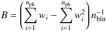 (1)where wi is the weight (probability) associated with the ith photon, nph is the total number of photons in the light curve, and nbin is the number of light-curve bins. The pulsar light-curve background represents the DC light-curve emission component that does not originate from the pulsars. The error associated with the jth phase bin of the light curve, corresponding to the standard deviation of the photon weights in that bin, is
 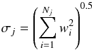 (2)where Nj is the number of photon weights in the jth bin. More details can be found in PSRCAT2.
The radio profiles of the RL LAT pulsars have been obtained in collaboration with the PSC and PTC. They have been built from observations mainly performed at 1400 MHz from Green Bank Telescope (GBT), Parkes Telescope, Nançay Radio Telescope (NRT), Arecibo Telescope, the Lovell Telescope at Jodrell Bank, and the Westerbork Synthesis Radio Telescope (Smith et al. 2008).
3. Simulation of the LAT pulsars emission patterns and light curves
3.1. Phase-plots
A pulsar phase-plot as a two-dimensional matrix, containing the pulsar emission at all rotational phases (light curve), for all the possible values of ζ, and obtained for the specific set of pulsar parameters: period P, surface magnetic field BG, gap width w, and α. For each of the LAT pulsars the pulsar BG and w of the various models have been computed as described in Pierbattista et al. (2012).
Let us define the instantaneous co-rotating frame (ICF) as the inertial reference frame instantaneously co-rotating with the magnetospheric emission point. The direction of the photon generated at the emission point in the pulsar magnetosphere as seen from an observer frame (OF) has been computed according to Bai & Spitkovsky (2010), as it follows: (i) the magnetic field in the OF has been computed as given by the retarded vacuum dipole formula; (ii) the magnetic field in the ICF has been computed by Lorentz transformation of the OF magnetic field; (iii) the direction of the γ-ray photons in the ICF, ηICF, has been assumed parallel to BICF; (iv) the direction of the γ-ray photons in the OF, ηOF has been computed by correcting ηICF for the light aberration effect.
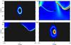 |
Fig. 1 Top left to bottom right panels: phase-plots obtained for the PC, SG, OG/OPC, and radio (core plus cone) models respectively, with a magnetic field strength of BG = 108 Tesla and spin period of 30 ms for the PC and radio cases, and gap widths of 0.04 and 0.01 for the SG and OG/OPC cases, respectively. All the plots are given for an obliquity α = 45°. The emission flux increases from black to red. |
We computed the γ-ray and radio phase-plots of each pulsar for the PC, SG, OG, and OPC γ-ray models and a radio core plus cone model. OPC and OG emission geometries are described by the same phase-plot. Examples of phase-plots are shown, for all the models, in Fig. 1.
In our computation, each phase-plot has been sampled in 45 × 90 steps in phase and ζ angle, respectively. Phase-plots were produced for every degree in α, from 1° to 90°. Given a pulsar phase-plot evaluated for a specific α, the light curve observed at a particular ζLTC is obtained by cutting horizontally across the phase-plot at constant ζLTC.
A detailed description of γ-ray models, radio model, and of the phase-plot generation strategy used in this paper can be found in Pierbattista et al. (2012).
3.2. Light-curves binning and normalisation
The simulated pulsar γ-ray light curves, generated as described in Sect. 3.1, are first computed in Regular Binning (RBin) where the phase interval 0 to 1 is divided into Nbin equal intervals and the light curve is built counting the photons in each bin. By fitting between RBin light curves, all the phase regions (peak or valleys) have the same statistical weight: in the case of significant pulsed emission over very few bins, the fit solution will be strongly dominated by the off-peak level and not by the pulsed emission. Since most of the observed LAT light curves exhibit emission concentrated in narrow peaks and a wide off-peak or bridge region, we increased the statistical weight of the peak regions by using fixed count binning (FCBin) light curves. In FCBin the size of each phase bin is re-defined in order to contain the same sum of weights per bin, obtained by dividing the total sum of weights by the total number of bins.
 |
Fig. 2 α-ζ log-likelihood maps obtained by fitting the γ-ray light curve of pulsar J1023−5746 with each γ-ray model phase plot. The fit has been performed with χ2 estimator and FCBin light curves. A white circle shows the position of the best-fit solutions. The colour-bar is in effective σ = ( | lnL − lnLmax | )0.5 units, zero corresponds to the best-fit solution. The diagonal band present in the PC panel is due to the fact that the emission region is located close to the polar cap and shines mainly when ζobs ≅ α. Elsewhere, for | ζobs − α | >ρ/ 2 with ρ the opening angle of the PC emission cone, no PC emission is visible from the pulsars and the simulated light curves for those angles are fitted as flat background emission. This generates the observed yellow flat field in the log-likelihood map. |
The simulated γ-ray light curves, obtained as described in Sect. 3.1, are computed in arbitrary intensity units and do not include background emission modelling. This means that before they are used to fit the LAT profiles, they must be scaled to the observed light curves, and a value for the background emission must be added.
Using the FCBin light curves helps the fit to converge to a solution making use of the main morphological information at its disposal: the level of pulsed to flat DC emission from the pulsar model and the level of flat background B from Eq. (1).
Let us define C as the normalisation constant of the simulated light curve. Imposing equality between the total photon count in the observed and modelled light curves yields an average constant Cbar near which the fit solution should converge: 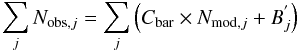 (3)where Nmod,j and Nobs,j are the j-bin values of the simulated and observed FCBin light curves respectively and
  is the background emission obtained from the constant background emission B computed in Eq. (1). Prior to being used in Eq. (3) both simulated light curve and background emission have been re-binned by applying the same binning technique as was used to obtain the observed light curve.
4. Radio-quiet pulsar (α,ζ) estimates: γ-ray fit only
We have used the PC, SG, and OG/OPC phase-plots and a χ2 estimator to fit the LAT pulsar γ-ray light curves sampled with RBin and FCBin in phase. The free parameters of the fits are: the α and ζ angles, both sampled every degree in the interval 1° to 90°; the final light-curve normalisation factor C sampled every 0.1Cbar in the interval 0.5Cbar to 1.5Cbar with Cbar from Eq. (3); the light-curve phase shift φ, sampled in 45 steps between 0 and 1.
For each type of light-curve binning, we have obtained a log-likelihood matrix of dimension 90α × 90ζ × 45φ × 11norm. Maximising the matrix over φ and C yields the α-ζ log-likelihood map. The location and shape of the maximum in this map give the best-fit estimates on α and ζ and their errors. An example of α-ζ log-likelihood map is given in Fig. 2 for the pulsar J1023−5746. The corresponding best-fit γ-ray light curve is shown in Fig. C.4. The comparison of the set of solutions obtained with the two light-curve binning modes shows that FCBin best matches the sharp peak structures of the observed profiles because of the higher density of bins across the peaks. Hereafter the α and ζ estimates given for RQ pulsars are those obtained with FCBin light curves. They are listed with their respective statistical errors in Table 1.
In order to estimate the systematic errors on the derivation of (α,ζ) due to the choice of fitting method, we have compared the sets of solutions obtained with the FCBin and RBin light curves. Their cumulative distributions give the errors at the 1σ and 2σ confidence levels displayed in Table 2. Because OG and OPC models predict sharp peaks and no off-pulse emission, we expect the differences between α and ζ obtained with RBin and FCBin light curves to be the largest with these models. It explains their large 2σ values in Table 2. The results in Table 2 most importantly show that the fitting method itself yields an uncertainty of a few degrees at least on α and ζ. It is generally much larger than the statistical errors derived from the log-likelihood map. For this reason we have set a minimum error of 1° in Table 1.
Figure 3 compares, for each pulsar, the relative goodness of the fit solutions obtained with the different models. The light curves from the modelled phase-plots can reproduce the bulk shape of the observed light curves, but not the fine details. Furthermore, the observed light curves having a large number of counts have very small errors. So the reduced χ2 values of the best fits remain large because the errors on the data are small compared to the model variance. On the other hand, the figures in Appendix C show that the optimum-models reasonably describe the light-curve patterns in most cases. To quantify the relative merits of the models, we have therefore set the model variance in order to achieve a reduced  of 1 for the optimum-model. This variance has then been used to calculate the value of other model solutions and to derive the
  difference between the optimum-model and any other model. In Appendix A, we show how to relate the original log-likelihood values obtained for each fit, given in Table C.1, and the differences between models.
Estimate of the systematic errors on α and ζ obtained from the comparison of the FCBin and RBin fits.
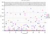 |
Fig. 3 Comparison of the relative goodness of the fit solutions obtained for the RQ LAT pulsars between the optimum-model and alternative models. The comparison is expressed as the |
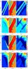 |
Fig. 4 For each model the (α,ζ) log-likelihood map for the γ-ray fit, the radio fit, and the sum of these two maps for pulsar J0205+6449 is shown. A white circle shows the position of the best fit solution for each log-likelihood map. The colour-bar is in effective σ = ( | lnL − lnLmax | )0.5 units, zero corresponds to the best-fit solution. |
The difference is plotted in Fig. 3 for each pulsar and each non-optimum-model. The χ2 probability density function for the 41 degrees of freedom of the fits gives us the confidence levels above which the alternative models are significantly worse. The levels are labelled on the plot. The results indicate that one or two models can be rejected for nearly half the pulsars, but we see no systematic trend against a particular model. We also note that the geometrically similar OG and OPC models give significantly different solutions in several instances. This is because the gap width evolves differently in the two models.
5. Radio-loud pulsar (α,ζ) estimates: fitting both the γ-ray and radio emission
The strategy we have adopted to jointly fit radio and γ-ray profiles consists of summing the log-likelihood maps obtained by fitting the radio and γ-ray light curves individually. Because of the much larger signal-to-noise ratio in the radio than in γ-rays, and since the γ-ray and radio models are equally uncertain, the radio log-likelihood map is more constraining and the joint fit is largely dominated by the radio-only solution. To lower the weight of the radio fit and make it comparable with the γ-ray fit we have implemented a two-step strategy: we have first fitted the radio profiles by using a standard deviation evaluated from the relative uncertainty in the γ-ray light curve. We have then used the best-fit light curves of this first fit to evaluate an optimised standard deviation in the radio and use it to fit again the radio light curves. A detailed description of the joint fit technique is given in Sects. 5.1 and 5.2.
5.1. Radio fit only
We have implemented a fit of the RBin radio profiles using 5 free parameters, the same four defined in Sect. 4, α, ζ, phase shift φ, and normalisation factor, equally stepped in the same intervals, plus a flat background emission level sampled in 16 steps over an interval that includes the averaged minimum of the observed light curve.
The first fit is done with the standard deviation σpeak evaluated as the average relative γ-ray uncertainty in the on-peak region times the maximum radio intensity value (Johnson et al. 2011; Venter et al. 2012). Hereafter we refer to this first fit as the σpeak radio fit. The second fit is implemented by using a standard deviation value evaluated from the best-fit results of the first fit, on the basis of a reduced χ2 = 1 criterion.
Let us define  the best fit light curve obtained in the first step which yields a maximum log-likelihood:
 ![Mathematical equation: \begin{equation} \label{opt1} \ln L_{\max}=-\frac{1}{2\sigma^2_{\gamma-\rm peak}}\sum_j \left[N_{{\rm obs},j}-N^{*}_{{\rm mod},j}\right]^2 \end{equation}](/articles/aa/full_html/2015/03/aa23815-14/aa23815-14-eq201.png) (4)with Lmax function of the best-fit α and ζ obtained from the first fit. By making use of the reduced χ2 = 1 criterion, Eq. (4) gives
(4)with Lmax function of the best-fit α and ζ obtained from the first fit. By making use of the reduced χ2 = 1 criterion, Eq. (4) gives ![Mathematical equation: \begin{equation} \label{RedChi2} \frac{1}{n_{\rm free}}\sum_j \frac{\left[N_{{\rm obs},j}-N^{*}_{{\rm mod},j}\right]^2}{\sigma_*^2}=1, \end{equation}](/articles/aa/full_html/2015/03/aa23815-14/aa23815-14-eq203.png) (5)where nfree = (nbin − 5) is the number of the free parameters and σ∗ is the newly optimised value for the standard deviation. Combining Eqs. (4) and (5) yields
(5)where nfree = (nbin − 5) is the number of the free parameters and σ∗ is the newly optimised value for the standard deviation. Combining Eqs. (4) and (5) yields 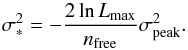 (6)The new optimised σ∗ is a function of the α and ζ solutions obtained in the first step. It has been used to implement a new fit of the radio light curves, hereafter the σ∗ radio fit.
5.2. Joint γ-ray plus radio estimate of the LAT pulsar orientations
Since the radio and γ-ray emissions occur simultaneously and independently, and since the γ-ray and radio log-likelihood maps have been evaluated in a logarithmic scale for the same free parameters, the joint (α,ζ) log-likelihood map is obtained by summing the γ-ray and radio maps.
We have summed the γ-ray log-likelihood maps, evaluated by fitting FCBin light curves (Sect. 4), with the radio log-likelihood maps, evaluated by fitting RBin light curves (Sect. 5.1) with either σpeak or σ∗. Among the two sets of solutions obtained for each pulsar, we have selected the solution characterised by the highest final log-likelihood value. An example of a joint γ-ray plus radio α-ζ estimate is given in Fig. 4 for the pulsar J0205+6449. The corresponding best-fit light curves are shown in Fig. D.1. The log-likelihood values L of the final results are listed in Table D.1.
Because of statistical fluctuations, and/or the difference in the radio and γ-ray profile accuracy, and/or the inadequacy of the assumed emission geometries to describe the data, the (α,ζ) solutions obtained from the joint fit did not always supply both radio and γ-ray emission at those angles. In those cases, the next highest log-likelihood (α,ζ) solution with non-zero radio and γ-ray pulsed emission was chosen. For some light curves with low statistics and/or signal-to-noise ratio, the joint fit method found a flat light curve as the best solution for the SG model. This is the case for pulsars J0729−1448, J1112−6103, J1801−2451, and J1835−1106. For those, we have selected the non-flat light curve with the highest log-likelihood value as the SG solution.
α and ζ best-fit solutions resulting from the joint radio plus γ-ray fit of the 41 RL pulsars.
Table 3 lists the (α,ζ) estimates obtained for the RL pulsars from the optimised σ∗ fit. Since the estimates are obtained by merging two 1° resolution log-likelihood maps, we conservatively assign a minimum statistical error of 2°. As for RQ pulsars in Sect. 4, we compare in Fig. 5 the relative goodness of the fits obtained between the optimum-solution and alternative models for the RL pulsars. We have derived the difference between two models according to Appendix A, by making use of the log-likelihood obtained for each fit and listed in Table D.1 and for 81 degrees of freedom. It shows that the tight additional constraint provided by the radio data forces the fits to converge to rather comparable light-curve shapes, so that the solutions often gather within 1σ from the optimum-solution. It also shows that the PC model is more often significantly rejected than the other, more widely beamed, models.
In order to estimate the systematic errors on the derivation of α and ζ, we have studied how the sets of solutions obtained with the two joint-fit methods (γ-ray fit plus σpeak radio fit and γ-ray fit plus σ∗ radio fit) depart from each other. Table 4 lists the 1σ and 2σ systematic errors on α and ζ for each model. It shows how the joint-fit strategy yields uncertainties of few degrees at least in α and ζ. They largely exceed the statistical errors shown in Table 3.
6. Results
For the RQ LAT pulsars, the best-fit light curves obtained by the fits in FCBin mode are shown in Figs. C.1 to C.18. while Figs. D.1 to D.41 show the radio and γ-ray best-fit light curves obtained from the joint γ-ray plus radio fits for the RL LAT pulsars. In Figs. E.1 and E.2 we give the joint radio plus γ-ray fit results for the RF pulsars J0106+4855 and J1907+0602. All radio light curves shown in Appendices have been plotted with the errors (optimised standard deviations σ∗) evaluated as described in Sect. 5.1. The α and ζ estimates for RQ and RL pulsars are indicated in Tables 1 and 3 respectively.
In addition to the χ2 fits to the FCBin and RBin γ-ray light curves described above, we have also tested maximum log-likelihood fits with Poisson statistics. We have checked that while the individual pulsar (α,ζ) estimates can change according to the method used, the collective properties of the LAT pulsar population discussed below, such as the correlation between luminosity and beaming factor with Ė, are robust and not strongly dependent on the fitting strategy.
Estimate of the systematic errors on α and ζ obtained from the comparison of the two joint fit methods γ-ray fit plus σpeak radio fit and γ-ray fit plus σ∗ radio fit.
6.1. Comparison of the γ-ray geometrical models
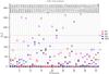 |
Fig. 5 Comparison of the relative goodness of the fit solutions obtained for the RL LAT pulsars between the optimum-model and alternative models. The comparison is expressed as the |
Left: for each model, the number (and frequency in the sample) of optimum-solutions that yield a better fit than the other models by at least 1σ. Right: for each model, the number and frequency of solutions that are rejected by more than 3σ compared to the optimum-model.
We can compare the merits of the models in terms of frequency of achieving the optimum-model in the sample of LAT pulsar light curves. Table 5 shows, for each model, the number of optimum-solutions that are better than the other models by at least 1σ (left) and the number of non-optimum-solutions that are rejected at more than 3σ (right). We give those counts for the RQ, RL, and all pulsars of the sample. Table 5 shows that, in the majority of cases, there is no statistically best optimum-solution. In the few cases where there are, most are SG and PC and only one is OPC. The PC emission geometry, in general, most poorly describe the observations; the PC model is rejected at more than 3σ confidence level for almost the 60% of the RL pulsars and for almost half of the total pulsars of the sample. The SG and PC models are rejected at more than 3σ nearly equally for RQ pulsars. Thus, the outer magnetosphere models, SG, OG and OPC, overall seem to best describe the observed LAT pulsar light curves. This geometrical trend concurs with the absence of a super-exponential cut-off in the recorded γ-ray spectra (PSRCAT2) to rule out a PC origin of the γ-ray beam in most of the LAT pulsars, but not all. We note that the RF and RQ pulsars J0106+4855 and J2238+5903 respectively, have a PC optimum-solution and that the other models are very strongly rejected. On the other hand, the PC optimum-solution obtained for pulsar J2238+5903 has α and ζ angles so close that it should be observed as RL or RF object and so it is likely to be incorrect, unless the radio emitting zone actually lies at higher altitude than in our present model. In any case, γ-ray beams originating at medium to high altitude in the magnetosphere largely dominate the LAT sample.
The fit results can point to which model best explains the emission from each pulsar but they do not single out a model that is able to explain all the observed light curves. This suggests that none of the assumed emission geometries can explain the variety of the LAT sample.
6.2. Impact of the radio emission geometry on the pulsar orientation estimate
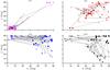 |
Fig. 6 Distribution of the α-ζ best-fit solutions obtained, for the RL pulsars sample and in the framework of each model, by fitting the γ-ray light curves alone (stars) and by jointly fitting the γ-ray and the radio light curves (squares). Recall that filled and empty symbols refer to the solutions of the optimum and alternative models, respectively. |
α and ζ best-fit solution resulting from the γ-ray only fit of the 41 RL pulsars.
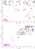 |
Fig. 7 α-ζ plane distribution of RQ (top panel) and RL (bottom panel) fit solutions for the PC (magenta triangles), SG (red circles), OG (blue squares), and OPC (black stars) models. Recall that filled and empty symbols refer to best-fit solutions of the optimum and alternative models, respectively. The optimum-solutions that are better than the other models by more than 1σ are plotted as light-colour-filled symbols. |
Figure 6 shows how the (α,ζ) solutions obtained for the RL sample migrate, from the γ-only solutions when we take into account the radio emission. We have used the χ2 fit and FCBin light curves to give an (α,ζ) estimate for RL Fermi pulsars based on the γ-ray emission only. They are listed in Table 6. We have plotted those solutions as stars in Fig. 6. To study how they change by including the radio emission in the fit, we have plotted as squares the solutions obtained with the joint σpeak radio fit and we have connected with a line the solutions of the two methods for each pulsar.
In many cases the γ-only solutions for RL pulsars are found far away from the diagonal (0,0) to (90,90) in the α-ζ plane where radio emission is more likely. Hereafter we refer to this diagonal as the radio diagonal. For all models except the PC, the introduction of the radio component in the fit causes the (α,ζ) solution to migrate from orientations where radio emission is unlikely toward the radio diagonal. This suggests that a γ-ray only fit estimate of α and ζ for RL pulsars may give results far away from the radio diagonal and should be used with caution.
In the PC model, the inclusion of the radio component in the fit produces a migration of the solutions along the radio diagonal. In the SG model, the extent of the migration is somewhat larger than in the PC case and it does not follow any trend (Fig. 6). In the OG and OPC models the γ-ray only solutions migrate the furthest to the joint solutions in Fig. 6. In the outer magnetosphere models, both the α and ζ angles can be underestimated according to the position of the γ-only solution with respect to the radio diagonal. When the γ-only solution is to the right of the radio diagonal, ζ migrates toward higher values while α keeps quite stable and vice versa when the γ-only solution is to the left of the radio diagonal.
6.3. α-ζ plane
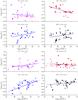 |
Fig. 8 Beaming factor fΩ versus the pulsar spin-down power Ė evaluated for RQ (top panel) and RL (bottom panel) pulsars . The lines represent the best power-law fits to the data points; the best fit power-law parameters with relative 1σ errors, are listed in Table 8. Hereafter the optimum-solutions that are better than the other models by more than 1σ will be plotted as light-colour-filled hexagrams. |
Figure 7 shows the solutions in the α-ζ plane for the RQ and RL pulsars in the top and bottom panels respectively. A comparison of the α and ζ estimates with the values obtained from observations at other wavelengths shows good consistency in all the reported cases (Tables 1 and 3). Our ζ estimates are consistent with the values predicted by Caraveo et al. (2003) for PSR J0633+1746 OG and OPC models, and with the values predicted by Ng & Romani (2008) for pulsars J0205+6449 OG/SG/OPC models, J1709−4429 OG model, J1833−1034 OG model, J2021+3651 SG model, and J2229+6114 OG model. For PSRs J1803−2149, Crab, and J1124−5916, none of our ζ estimates is included in the interval predicted by other authors. For those pulsars, the values closest to the predictions made by Ng & Romani (2008) are obtained by OG for J1803−2149, SG/OG/OPC for the Crab, and by all models for J1124−5916. In the case of the Vela pulsar, our SG model predictions α = 45° ± 2° and ζ = 69° ± 2° are both consistent with α = 43° by Johnston et al. (2005) and 63° ≲ ζ ≲ 64° by Ng & Romani (2008).
Since the radio and PC emissions are generated in the same region of the magnetosphere in narrow conical beams, coaxial with the magnetic axis, all the PC solutions are found along the radio diagonal. The concentration of solutions at low α and ζ for both RQ and RL pulsars is due to the PC emission geometry, for which low α and ζ angles predict the highest variety of light-curve shapes.
The majority of SG solutions, both for RQ and RL objects, are concentrated in the central-upper part of the radio diagonal. The paucity of low α and ζ solutions is due to SG geometry: the SG bright caustics shine generally at high ζ and tend to concentrate toward the neutron star spin equator as α decreases.
Beaming factors fΩ evaluated for the RQ (left) and RL (right) pulsars in the framework of each model.
In agreement with Takata et al. (2011) we show that OG and OPC solutions for both RQ and RL pulsars are mainly observed at high α and ζ angles, preferably at high ζ for all obliquities for the RQ pulsars. Only a handful of OPC pulsars are potentially seen at ζ< 30°. The comparison of OG and OPC solutions shows that the two different prescriptions for the gap width evolution do not much affect the estimation of α and ζ. The fact that RQ SG solutions are closer to the radio diagonal than RQ OG solutions is due to their different emission geometry: two-pole emission geometry (emission from both poles, e.g. Two Pole Caustic model, Dyks & Rudak 2003) and one-pole emission geometry (emission from just one pole, Outer Gap model, Cheng et al. 2000) respectively. It follows that for lower α angles (≲ 45°), OG emission can be observed with large enough peak separation only at high ζ angles whereas in the SG geometry large peak separations can be observed at lower ζ angles and from both poles.
We show in Fig. B.1 the α-ζ plane distribution obtained for the γ-ray visible pulsars from the population synthesis described in Pierbattista et al. (2012). The comparison with the RQ and RL pulsars of Fig. 7 shows consistency between the LAT pulsars and the prediction from the Galactic population for the SG, OG, and OPC models. The PC predictions show an abundance of solutions at intermediate (α,ζ) that are not observed in the LAT sample.
We now use the (α,ζ) solutions to study various collective properties of the LAT pulsar sample.
6.4. Beaming factor fΩ
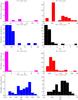 |
Fig. 9 Beaming factor fΩ distribution for the RQ (top panel) and RL (bottom panel) pulsars and all models. |
The pulsar beaming factor fΩ is the ratio of the total luminosity radiated over a 4π sr solid angle to the observed phase-averaged energy flux, 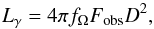 (7)where D is the pulsar distance and Fobs is the observed pulsar flux. The LAT pulsar beaming factors fΩ have been evaluated from each of the (α,ζ) solutions and the corresponding phase-plots according to:
 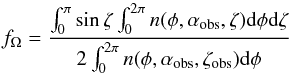 (8)where the numerator is the integrated luminosity radiated by the pulsar in all directions for the αobs obliquity and the denominator integrates the energy flux intercepted for the observer line of sight ζ = ζobs (Watters et al. 2009).
Figure 8 shows the beaming factor as a function of the pulsar spin-down power. The beaming factors have been derived from the best-fit RQ and RL (α,ζ) solutions for each model. The LAT pulsar spin-down powers Ė have been evaluated from the periods and period first time derivatives given in PSRCAT2, as described in Pierbattista et al. (2012) (with a different choice of pulsar moment of inertia, mass, and radius than in PSRCAT2). The dependence of the beaming factors on Ė have been fitted, using a nonlinear regression algorithm, with power laws, the indices of which are given in Table 8. The goodness of each fit shown in Table 8 has been estimated by computing the coefficient of determination R2 that compares the sum of the squares of residuals and the dataset variability (proportional to the sample variance). It is computed as 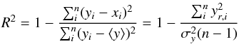 (9)where yi are the data, xi are the fit predictions, yr,i are the fit residuals,
  is the data sample variance, ⟨ y ⟩ is the average value of the data sample, and n is the number of data points in the fit. R2 ranges between 0 and 1 and a value close to 1 indicates a good correlation between data and fit predictions.
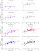 |
Fig. 10 γ-ray luminosity versus Ė for RQ (top panel) and RL (bottom panel) Fermi pulsars. The thick lines represent the best power-law fits to the data points; their parameters and 1σ errors are listed in Table 8. The thin dot-dashed line indicates 100% conversion of Ė into γ-rays. |
In the PC case fΩ is low as expected from the small hollow cone beam produced above the polar caps (Fig. 1). The fΩ distribution is centred around 0.05 and 0.07 for RQ and RL objects, respectively. Since the PC beam size scales with the polar cap size, we expect fΩ to decrease as the period increases, thus as Ė decreases. Because of the high dispersion in the sample, no trend is apparent. In the SG case, the beaming factor of both RL and RQ pulsars remains rather stable and well constrained around fΩ ~ 1. A more pronounced fΩ-Ė correlation, characterised by a higher index of determination R2 (Table 8), is observed for the RQ pulsars. The absence of an evident correlation between fΩ and Ė is due to the less strongly beamed nature of the SG emission, to the high level of off-pulse emission predicted, and on the fact that, contrary to the OG, the bright caustics do not quickly shrink toward the pulsar equator as the pulsar ages, but they span a wider range of ζ values. In the OG and OPC cases, the fΩ values are much less dispersed for the RL pulsars than for the RQ pulsars as indicated in Pierbattista et al. (2012). Both OG and OPC do not show any significant fΩ variation for RQ pulsars with Ė and are characterised by distributions centred around ~0.25 and ~0.64 for RQ and RL OG objects respectively, and ~0.41 and ~0.85 for RQ and RL OPC objects respectively. The OG model exhibits a more pronounced fΩ-Ė correlation, characterised by a higher index of determination R2 (Table 8), for RL pulsars. The distribution of the beaming factor values in the framework of each model is shown in Fig. 9. In all models other than the SG, the beaming factors calculated for the RQ population are numerically smaller than those calculated for the RL population. This is consistent with the fact that the wide SG γ-ray beams of the RL pulsars have higher probability to overlap the radio beams. The beaming factors for RQ and RL LAT pulsars computed in the framework of each model are given in Table 7. The fΩ values are generally lower than one for all models and this suggests that to assign a beaming factor of one to all the pulsars (as done in PSRCAT2) is likely to represent an overestimation of the real values.
6.5. Luminosity
Figure 10 shows the γ-ray luminosity versus Ė for RQ and RL pulsars in the upper and lower panel respectively. The γ-ray luminosities of the LAT pulsars have been computed with Eq. (7) by using the pulsar fluxes detected by the LAT above 100 MeV (PSRCAT2), and the beaming factor fΩ computed from the simulated phase plot with Eq. (8). The error on the LAT luminosities include the errors on the LAT fluxes and distances as listed in PSRCAT2. The correlations between γ-ray luminosities and Ė have been fitted, using a nonlinear regression algorithm, with power laws, the indices and coefficient of determination R2 of which are given in Table 8.
Best power-law fits to the distribution of fΩ and Lγ as functions of Ė for each model and RL or RQ pulsars.
For RQ and RL objects of all models, the trend  , observed in the first LAT pulsar catalogue (Abdo et al. 2010b) and confirmed in PSRCAT2, is observed within the errors. The luminosity excess (Lγ>Ė) observed in PSRCAT2 for some pulsars is solved here by computing each pulsar beaming factor from its best-fit light curve and emission pattern phase-plot (Eq. (8)). The only exception is noted for the PC luminosity of PSR J2021+4026 but this results is likely incorrect since this pulsar appears to have a low | α − ζ | and should be observed as RL or RF object. Moreover, the γ-ray luminosity distribution as a function of Ė, evaluated in the framework of each model, appears much less dispersed than in PSRCAT2. The lack of objects with Lγ>Ė, using our fΩ estimate, supports the conclusion that to assign a beaming factor of 1 to all the pulsars represents an overestimate of the real value, particularly for low Ė pulsars. The distributions observed in Fig. 10 for RL pulsars are consistent with the model prediction shown in Pierbattista et al. (2012), with the PC model providing the lowest luminosity values and SG and OG distributions characterised by the same dispersion.
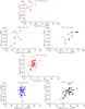 |
Fig. 11 Geometric γ-ray luminosity, Lgeo versus the standard gap-model γ-ray luminosity Lrad for RQ (top panel) and RL (bottom panel) Fermi pulsars and each model. The dot-dashed lines indicates Lgeo = Lrad. |
Figure 11 shows the geometric γ-ray luminosity of the LAT pulsars computed with Eqs. (7) and (8), Lgeo, as a function of the standard gap-model γ-ray luminosity computed as Lrad = W3Ė. In some cases Lgeo overestimates Lrad by more than 2 orders of magnitude for RQ pulsars and 3 orders of magnitude for RL pulsars. This is mainly the case for small gap-width pulsars, W< 0.1, that are expected to shine with Lrad< 0.001Ė but that show larger γ-ray luminosities Lgeo. This inconsistency reflects the difficulties in defining a unique gap width that could simultaneously explain the light-curve shape and the observed pulsar flux in the framework of the same radiative-geometrical model: the observed γ-ray pulsar light-curve shapes are well explained by thin gaps that yet do not provide enough luminosity to predict the observed γ-ray flux. The radiative-geometrical luminosity discrepancy appears more pronounced for the SG pulsars, where the gap-width computation critically depends on the assumed shape of the pair formation front (PFF; see description of the λ parameter in Pierbattista et al. 2012, Sect. 5.2). In the OG model, Lgeo overestimates Lrad just for RQ pulsars while the Lgeo of RL objects are more distributed around 100% of Lrad but showing a large dispersion above Lrad. The OPC is the model that shows the highest agreement between geometrical and radiative luminosity estimates with both RQ and RL Lgeo homogeneously distributed around 100% of Lrad. This is expected since the OPC luminosity law is artificially designed to match observed luminosities.
Pierbattista et al. (2012) reduced the lack of Lrad discrepancy by choosing the highest possible γ-ray efficiency, 100%, for the OG model and by choosing an appropriate PFF shape (see Sect. 5.2 of Pierbattista et al. 2012) and by setting the γ-ray efficiency to 1200% for the SG model. The high SG efficiency is possibly justified by the enhanced accelerating electric field expected in case of offset polar caps (Harding & Muslimov 2011).
The geometrical approach adopted in this paper avoid the lack of Lrad obtained for SG and OG models (Pierbattista et al. 2012) when one tries to simultaneously explain light-curve shape and luminosity and does not require ad-hoc γ-ray efficiency assumptions. On the other hand our geometrical approach highlights an intrinsic inconsistency between geometric and radiative models in describing the pulsar magnetosphere. The geometrical model used in this paper is based on simple assumptions that do not account for the complex electrodynamics at the base of the radiative gap-models. This is true for both OG and SG models and cause the radiative-geometrical luminosity inconsistencies discussed above. The OG model requires large gap widths to produce the observed luminosities, and these gaps do not produce the observed thin light-curve peaks. This is suggested by the higher consistency between radiative and geometrical luminosities obtained by the OPC model that differs from the OG just in the gap-width formulation. In the SG model, radiative-geometrical luminosity inconsistencies are due to two factors: thin slot gaps required to explain the light-curve shapes do not produce enough luminosity to explain the observed fluxes; the electrodynamics of the low-altitude slot-gap region is not implemented in the adopted geometrical model. The assumptions on the SG high-altitude emission and the inconsistencies between radiative and geometrical SG emission at low altitude are discussed in Sect. 6.7.1.
In the current formulation of SG and OG geometrical models, both SG and OG model acceleration and emission regions are restricted to inside the light cylinder. In more recent and realistic global dissipative pulsar magnetosphere models, acceleration and emission also outside the light cylinder may be able to solve this radiative-geometrical luminosity discrepancy (Kalapotharakos et al. 2014; Brambilla et al., in prep.).
6.6. Magnetic alignment and pulsar orientation
Figure 12 shows α versus the characteristic age τch for each model and pulsar type. We have tried to verify if the LAT sample shows any evidence of an alignment or misalignment of the magnetic and rotational axes with age. The possibility that magnetic and rotational axes of a pulsar could become aligned with time has been suggested by Young et al. (2010) on the basis of a pulsar evolution model including two distinct effects: an exponential magnetic alignment as indicated by Jones (1976) and a progressive narrowing of the emission cone as the pulsar ages. The alignment of magnetic and rotational axes of a pulsar should occur on a timescale of ~ 106 yr.
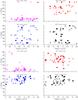 |
Fig. 12 Magnetic obliquity α versus characteristic age for RQ (top panel) and RL (bottom panel) Fermi pulsars and each model. |
Both RQ and RL solutions for all the models are highly dispersed and show no evidence of changes in α with age. In Fig. 13 we show gap width as a function of α for RQ and RL pulsars for all models. A mild dependence between gap width and α is present just for the OG model and is due to the fact that in the OG model the gap width wOG is a function of α.
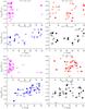 |
Fig. 13 Gap width as a function of α for RQ (top panel) and RL (bottom panel) Fermi pulsars and each model. |
Figure 14 shows the quantity | α − ζ | plotted as a function of the pulsar period, for RQ and RL pulsars in all models. It is evident how the solutions change from RQ to RL objects, appearing much less dispersed and showing slight decreasing trends with the spin period. This trend is due to a selection effect for which young and rapidly spinning pulsars have a wider radio beam that can overlap the γ-ray beam up to high | α − ζ | values. As a pulsar ages, its spin period increases while polar cap size and radio beam size decrease and the radio beam will overlap the γ-ray beam only for smaller | α − ζ |. This trend is consistent with changes of | α − ζ | as a function of the spin period, obtained, for each emission model, in the population synthesis study described in Pierbattista (2010) and shown in Fig. 6.84 of that paper.
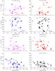 |
Fig. 14 For each model the β = | α − ζ | angles a function of the spin period for RQ (top panel) and RL (bottom panel) Fermi pulsars is shown. |
Best power-law fits to the distribution of Ecut and Γ as functions of the width of the acceleration gap for each model and RL or RQ pulsars.
6.7. High-energy cutoff and spectral index versus gap width
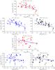 |
Fig. 15 Energy cutoff versus gap width for RQ (top panel) and RL (bottom panel) Fermi pulsars for each model. The best fit power law trends are given in each figure. PC and SG results are characterised by the same gap width wSG and have been plotted together. |
Figures 15 and 16 show the relation between observable spectral characteristics, namely the high-energy cutoff Ecut and spectral index Γ, and the width of the emission gap evaluated in the framework of each emission model. Γ and Ecut are taken from PSRCAT2. The SG, OG, and OPC gap widths have been calculated for each pulsar according to its spin characteristics as described in Pierbattista et al. (2012).
The spectral fits for the RL pulsars J1410−6132, J1513−5908, and J1835−1106 were noted as unreliable in PSRCAT2. These pulsars are not included in Figs. 15 and 16. We find a tendency for Ecut and Γ to decrease when the gaps widens. This dependence is particularly important because it relates the spectral characteristics and the intrinsic, non-directly observable, gap width that controls the acceleration and cascade electrodynamics.
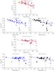 |
Fig. 16 Spectral index versus gap width for RQ (top panel) and RL (bottom panel) Fermi pulsars for each model. The best fit power law trends are given in each figure. PC and SG results are characterised by the same gap width wSG and have been plotted together. |
A power law dependence between Ecut and SG, OG, and OPC gap widths can be theoretically obtained as it follows (see Fig. 15 and Table 9 for comparison). From Abdo et al. (2010a), the Ecut dependence is defined as  (10)where E∥ is the electric field parallel to the magnetic field B lines, and ρc is the radius of curvature of the magnetic field lines. Since for all the implemented emission models E∥ scales as E∥ ∝ w2BLC, we have
 ![Mathematical equation: \begin{equation} E_\mathrm{cut}\propto \left[w^2 B_\mathrm{LC}\right]^{3/4} \rho_{\rm c}^{1/2} \end{equation}](/articles/aa/full_html/2015/03/aa23815-14/aa23815-14-eq514.png) (11)where w is the width of the emission gap. The light cylinder magnetic field dependence can be written as
(11)where w is the width of the emission gap. The light cylinder magnetic field dependence can be written as 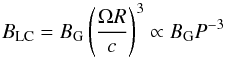 (12)with R the pulsar radius. Since, for SG, OG, and OPC the γ-ray emission occurs mainly at high altitude, close to the light cylinder, ρc ∝ RLC ∝ P, and the Ecut proportionality can be expressed as
 ![Mathematical equation: \begin{equation} E_\mathrm{cut}\propto w^{3/2} \left[P B_\mathrm{G}^{-3/7}\right]^{-7/4}. \label{EcutRef} \end{equation}](/articles/aa/full_html/2015/03/aa23815-14/aa23815-14-eq518.png) (13)Since the slot gap width dependence follows approximately
(13)Since the slot gap width dependence follows approximately 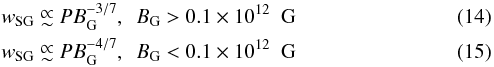 the final approximate Ecut,SG = f(wSG) dependence is
 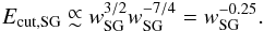 (16)More approximated power law dependences between Ecut and the OG and OPC gap widths can also be obtained from Eq. (13) and from the wOG and wOPC dependences. From Pierbattista et al. (2012) we have that wOG can be written as
![Mathematical equation: \begin{eqnarray} &&w_\mathrm{OG}\propto B_\mathrm{G}^{-4/7}P^{26/21}=\left[B_\mathrm{G}^{-3/7}P^{13/14}\right]^{4/3}\approx \left[B_\mathrm{G}^{-3/7}P\right]^{4/3}\label{OGnew}\\ &&w_\mathrm{OPC}\propto \dot{E}^{-0.5}=B_\mathrm{G}^{-1}P^{2}=\left[B_\mathrm{G}^{-3/7}P^{6/7}\right]^{7/3}\approx \left[B_\mathrm{G}^{-3/7}P\right]^{7/3} \label{OPCnew} \end{eqnarray}](/articles/aa/full_html/2015/03/aa23815-14/aa23815-14-eq523.png)
where the right-hand member of Eq. (17) has been obtained under the assumption P13/14 ≈ P, while the right-hand member of Eq. (18) has been obtained by making use of the relations Ė ∝ ṖP-3 and  , and by assuming P6/7 ≈ P. By solving Eqs. (17) and (18) for
 ![Mathematical equation: \hbox{$[B_\mathrm{G}^{-3/7}P]$}](/articles/aa/full_html/2015/03/aa23815-14/aa23815-14-eq528.png) and substituting in Eq. (13) we obtain the final approximate Ecut,OG = f(wOG) and Ecut,OPC = f(wOPC) dependences
and substituting in Eq. (13) we obtain the final approximate Ecut,OG = f(wOG) and Ecut,OPC = f(wOPC) dependences 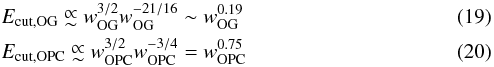 In Figs. 15 and 16, nonlinear regression power-law fits to all the data points are given for both pulsar types and all models. The fit indices and coefficients of determination R2 are given in Table 9.
 |
Fig. 17 Variation, in a force-free magnetosphere, of the ratio Goldreich-Julian charge density over the magnetic field, ρGJ/B, with the distance from the pulsar expressed in unit of the light-cylinder radius, r/RLC. |
Figure B.2 shows the behaviour of Ecut and Γ with respect to the SG, OG, and OPC gap widths for the population synthesis results in Pierbattista et al. (2012). The fact that no trend is apparent is due to the choice of spectral characteristics that have been randomly assigned from the double gaussian distribution that statistically describes the observed values in the LAT catalogue. The fact that the results in Figs. 15 and 16 show a trend that can be predicted theoretically encourages future efforts to confirm the trend and to improve the implemented fit strategy. Since in the phase-plot modelling there is no relation between Ecut and gap width, our results suggest a real physical relation between the γ-ray spectrum and gap width that can be used to discriminate between the proposed models. Moreover, the lack of trend in the simulation data for both Ecut and Γ (Figs. B.2) demonstrates that the decline observed in the present LAT sample is not due to an observation bias. A more precise Ecut = f(w) relation drawn from the analysis of a larger LAT sample should be tested in the future for both young and millisecond pulsars.
6.7.1. The SG γ-ray emission
The SG width computation implemented in this paper follows the prescription by Muslimov & Harding (2004). Those authors assumed that the Goldreich-Julian charge density, ρGJ (Goldreich & Julian 1969), does not grow monotonically up to the light cylinder, as it would happen in the case of a dipolar magnetic field, but it levels off at high altitudes. The growing of ρGJ depends on the field line curvature that in a force free magnetosphere decreases toward the light cylinder (the poloidal magnetic field lines tend to get straighter) so causing the levelling off of ρGJ. Recent implementations of force free magnetosphere pulsar models show that, at high altitudes, the variation of ρGJ with the distance from the pulsar is consistent with the assumption from Muslimov & Harding (2004). In Fig. 17 the variation of the quantity ρGJ/B with B the pulsar magnetic field, as a function of the distance from the pulsar in units of RLC is shown. It shows how the quantity ρGJ/B levels-off at distances larger than 0.4 RLC.
At low altitudes, typically < 0.4RLC, the physical SG model predicts a reversal of the sign of E∥ on some magnetic field lines and for some α values and no straightening of the low-altitude magnetic field lines is assumed. In the current implementation of the SG emission geometry no reversal of the sign of E∥ and no straightening of the magnetic field lines at low altitude are implemented: our modelling of the SG geometry assumes a simplified low-altitude slot-gap region and emission is assumed from all field lines in the gap. The impact of our simplified prescription for the SG structure in the current paper may be an overestimation of the geometric γ-ray luminosity, Lgeo, for those pulsars with very high α. However the actual impact of our assumption on the estimate of Lgeo could be quantified just through the future implementation of a geometric model that accounts for the reversal of the sign of E∥ in the low-altitude slot gap.
7. Summary
We have selected a sample of young and middle-aged pulsars observed by the LAT during three years and described in PSRCAT2. We have fitted their γ-ray and radio light curves with simulated γ-ray and radio emission patterns. We have computed the radio emission beam according to Story et al. (2007) and we have used the geometrical model of Dyks et al. (2004) to simulate the γ-ray emission according to four gap models, PC, (Muslimov & Harding 2003), SG, (Muslimov & Harding 2004), OG, (Cheng et al. 2000) and OPC (Romani & Watters 2010; Watters et al. 2009). Each emission pattern has been described by a series of phase-plots, evaluated for the pulsar period, magnetic field, and gap width, and for the whole α interval sampled every degree. These phase-plots predict the pulsar light curve as a function of ζ.
The simulated phase-plots have been used to fit the observed radio and γ-ray light curves according to two different schemes: a single fit to the γ-ray profiles of RF and RQ objects and a joint fit to the γ-ray and radio light curves of RL pulsars.
The individual fit to the γ-ray profiles has been implemented using a χ2 estimator and light curves binned both in FCBin and RBin. The comparison of the results obtained with the two methods shows that the χ2 fit with FCBin light curves yields the closest match between the observations and modelled profiles. We use the latter to give α and ζ estimates for the RQ and RF LAT pulsars and we use the RBin fit to evaluate the systematic uncertainties induced by the fitting method.
The joint γ-ray plus radio fit of RL pulsars uses RBin radio light curves and FCBin γ-ray light curves with a χ2 estimator. The log-likelihood maps in α and ζ obtained from the radio-only and γ-ray-only fits were summed to produce the joint solution. Two options were considered to couple the high signal-to-noise ratio of the radio data to the much lower signal-to-noise ratio of the γ-ray profiles and the solution characterised by the highest log-likelihood value was selected. The systematic errors on (α,ζ) for the RL pulsars have been obtained by studying the difference between the solutions obtained with the two joint fit coupling schemes.
We have obtained new constraints on α and ζ for 33 RQ, 2 RF, and 41 RL γ-ray pulsars. We have studied how the (α,ζ) solutions of RL pulsars obtained by fitting only the γ-ray light curves change by including the radio emission in the fit. We have used the α and ζ solutions to estimate several important pulsar parameters: gap width, beaming factor, and luminosity. We have also investigated some relations between observable characteristics and intrinsic pulsar parameters, such as α as a function of age and the spectral energy cut-off and index in γ-rays as a function of the gap width. We find no evidence for an evolution of the magnetic obliquity over the ~ 106 yr of age span in the sample, but we find an interesting apparent change in the γ-ray spectral index Γ and high-energy cutoff Ecut associated with changes in the gap widths.
We have found that a multi-wavelength fit of γ-ray and radio light curves is important in giving a pulsar orientation estimate that can explain both radio and γ-ray emission. The PC emission geometry explains only a small fraction of the observed profiles, in particular for the RL pulsars, while the intermediate to high SG and OG/OPC models are favoured in explaining the pulsar emission pattern of both RQ and RL LAT pulsars. The fact that none of the assumed emission geometries is able to explain all the observed LAT light curves suggests that the true γ-ray emission geometry may be a combination of SG and OG and that we detect the respective light curves for different observer viewing angles.
Comparison of the α and ζ solutions obtained by fitting only the γ-ray profiles of RL pulsars and both their γ-ray and radio profiles suggests that in the OG and OPC models, α or ζ are underestimated when one does not account for radio emission. When the γ-only solution is to the right of the radio diagonal in the α-ζ plane, ζ migrates toward higher values while α keeps quite stable and vice versa when the γ-only solution is to the left of the radio diagonal.
The beaming factors found for the RQ and RL objects are consistent with the distributions obtained in the population study of Pierbattista et al. (2012). For all the models we observe a large scatter of the beaming factors with Ė, which is reduced for RL pulsars compared to RQ pulsars, except for the SG. This is because RQ pulsars are viewed at lower α and ζ, and OG and OPC beams shrink towards the spin equator with decreasing Ė while SG beams do not. The low fΩ values found for the PC reflect the narrow geometry of the PC beams. The fΩ values for the SG appear to be fairly stable around 1 over 4 decades in Ė. We find also little evolution for the OG and OPC beaming factors of RQ objects which gather around 0.25 and 0.41, respectively. Larger averages are obtained for the RL objects (0,64 for OG and 0,85 for OPC) with no evolution with Ė for the OPC case and some hint of an increase with Ė in the OG case. The fact that the majority of the pulsars exhibit an fΩ estimate less than unity in all models suggests that the isotropic luminosities (fΩ = 1) often quoted in other studies are likely to overestimate the real values.
For all the models a power law relation consistent with  is observed for both RQ and RL pulsars. In contrast with PSRCAT2 we do not obtain any γ-ray luminosities significantly higher than Ė. Since the only difference between the luminosity computation here and that of PSRCAT2 is in the fΩ value (assumed equal to one in the catalogue), the excessively high luminosities obtained in the catalogue probably result from a too high beaming factor. We have studied the consistency of the geometric γ-ray luminosity, Lgeo, obtained in this paper and the γ-ray luminosity computed in the framework of radiative gap-models, Lrad. We found that Lgeo overestimate Lrad of 2−3 order of magnitude for the RQ and RL SG pulsar and for RQ OG pulsars while the Lgeo of RL OG objects are more consistent with their Lrad values while showing higher dispersion in Lgeo. For both RQ and RL OPC objects, Lrad is consistent with the Lrad estimates. These OG and SG geometric-radiative luminosity disagreements are due to inconsistencies in the formulation of the geometrical and radiative aspects of the γ-ray pulsar emission, rise the problem of formulating geometrical models more based on the actual pulsar electrodynamics in the framework of each gap model, and points to fundamental shortcomings of these electrodynamic gap models.
We find a correlation between Ecut and Γ of the γ-rays and the accelerator gap width in the magnetosphere. The relation is consistent with the SG prediction  just for the RL objects while the more approximated predictions formulated for OG and OPC models are not consistent with the observations. This Ecut and Γ versus gap width proportionality is important because it connects the observed spectral information and the non observable size of the gap region on the basis of the light-curve morphology alone.
Online material
Appendix A: Estimate of the goodness of the fit for each model solution
In this Appendix we describe the calculations used to quantify the relative goodness of the fit solutions obtained between the optimum-model and another model. The method assumes that the optimum-model light curve describes reasonably well the observations and it is based on the evaluation of the standard deviation of all the models, σ⋆, by imposing that the reduced of the optimum-solution is equal to unity. The difference between the values reached for the optimum-model and the other models then provides a measure of the relative goodness of the two solutions.
The χ2 of the optimum-model and of another model,  and
and  respectively, are defined as
 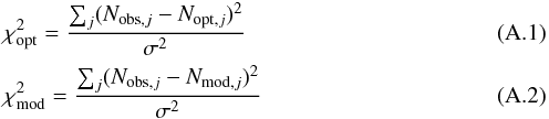 where Nobs,j and Nmod,j are the observed and modelled light curves respectively, and σ the standard deviation of the observed light curve. The difference between these two χ2 can be evaluated from the log-likelihood values given in Tables C.1 and D.1 as Δχ2 = −2 [ln(Lopt) − ln(Lmod)].
With the reduced χ2 of the optimum model set to 1, the standard deviation of the models, σ⋆, is  (A.3)
(A.3)
where Nd.o.f. is the number of degrees of freedom of each type of fit (41 for RQ pulsars and 81 for RL pulsars). With the model variance, the of the optimum and other models become: ![Mathematical equation: \appendix \setcounter{section}{1} \begin{eqnarray} \chi^2_{\rm opt,\star} &=& N_{\rm d.o.f.} \label{4} \\[2mm] \chi^2_{\rm mod,\star} &=& N_{\rm d.o.f.}\frac{\sum_j (N_{{\rm obs},j}-N_{{\rm mod},j})^2}{\sum_j (N_{{\rm obs},j}-N_{{\rm opt},j})^2} \label{5} \end{eqnarray}](/articles/aa/full_html/2015/03/aa23815-14/aa23815-14-eq550.png) and their difference
and their difference  is
is ![Mathematical equation: \appendix \setcounter{section}{1} \begin{eqnarray} \Delta\chi^2_\star &= \chi^2_{\rm mod,\star} - \chi^2_{\rm opt,\star} \nonumber\\[1.5mm] &= & {1\over \sigma^2_\star}\left[\sum_j (N_{{\rm obs},j}-N_{{\rm mod},j})^2 - \sum_j (N_{{\rm obs},j}-N_{{\rm opt},j})^2 \right]\notag \\[1.5mm] &=& N_{\rm d.o.f.} \frac{\sum_j (N_{{\rm obs},j}-N_{{\rm mod},j})^2 - \sum_j (N_{{\rm obs},j}-N_{{\rm opt},j})^2}{\sum_j (N_{{\rm obs},j}-N_{{\rm opt},j})^2} \notag \\[1.5mm] & = & N_{\rm d.o.f.} \left(\frac{\chi^2_{\rm mod}-\chi^2_{\rm opt}}{\chi^2_{\rm opt}}\right) \cdot \label{6} \end{eqnarray}](/articles/aa/full_html/2015/03/aa23815-14/aa23815-14-eq552.png) (A.6)We have plotted the resulting values in Figs. 3 and 5. The 1σ, 3σ, and 5σ confidence levels plotted in these figures have been obtained from the χ2 probability density function for the appropriate number of degrees of freedom.
(A.6)We have plotted the resulting values in Figs. 3 and 5. The 1σ, 3σ, and 5σ confidence levels plotted in these figures have been obtained from the χ2 probability density function for the appropriate number of degrees of freedom.
Appendix B: Population synthesis results from Pierbattista et al. (2012)
By synthesising a pulsar population we compared theoretical and observed distributions of observable quantities between the Fermi pulsars and the predictions of different γ-ray models. We have assumed low/intermediate and high-altitude magnetosphere emission models PC and SG, OG and OPC respectively, and core plus cone radio emission model. Full details on the population synthesis study can be found in Pierbattista et al. (2012). The plots shown in this Appendix have been obtained as additional results to the population study in Pierbattista et al. (2012) by using the original data at our disposal.
Appendix B.1: α-ζ plane
The α and ζ distributions of the visible component of the simulated population for PC, SG, OG, and OPC models are shown.
Appendix B.2: High-energy cutoff and spectral index as a function of the gap width
High energy cutoff and spectral index as a function of the width of the accelerator gap of the visible component of the simulated population for PC, SG, OG, and OPC. In disagreement with Fig. 15, no Ecut-gap width dependence is predicted from the simulations.
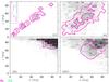 |
Fig. B.1 Number density of the visible γ-ray pulsars obtained for each model as a function of α and ζ in the population synthesis of Pierbattista et al. (2012). The linear grey scale saturates at 1.5 star/bin. The pink contours outline the density obtained for the radio-loud γ-ray sub-sample (at 5% and 50% of the maximum density). The insert gives the set of ζ values measured by Ng & Romani (2008) from the orientation of the wind torus seen in X rays (pink lines) and by Caraveo et al. (2003) from the orientation of the Geminga X-ray tails (green line). The separation in α in the insert is meaningless. |
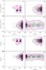 |
Fig. B.2 Number density of the visible γ-ray pulsars obtained for each model as a function of gap width and high-energy cutoff (left) and of gap width and spectral index (right). The linear grey scale saturates at 8 star/bin. The pink contours outline the density obtained for the radio-loud γ-ray sub-sample (at 5% and 50% of the maximum density). |
Appendix C: The LAT pulsar γ-ray fit light-curve results
Best fit log-likelihood values resulting from the γ-ray fit of the 35 RQ pulsars of the analysed sample.
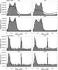 |
Fig. C.1 Top: PSR J0007+7303; bottom: PSR J0106+4855. For each model the best γ-ray light-curve (thick black line) is superimposed on the LAT pulsar light-curve (shaded histogram). The estimated background is indicated by the dash-dot line. |
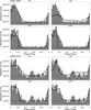 |
Fig. C.2 Top: PSR J0357+3205; bottom: PSR J0622+3749. For each model the best γ-ray light-curve (thick black line) is superimposed on the LAT pulsar light-curve (shaded histogram). The estimated background is indicated by the dash-dot line. |
 |
Fig. C.3 Top: PSR J0633+0632; bottom: PSR J0633+1746. For each model the best γ-ray light-curve (thick black line) is superimposed on the LAT pulsar light-curve (shaded histogram). The estimated background is indicated by the dash-dot line. |
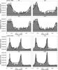 |
Fig. C.4 Top: PSR J0734-1559; bottom: PSR J1023-5746. For each model the best γ-ray light-curve (thick black line) is superimposed on the LAT pulsar light-curve (shaded histogram). The estimated background is indicated by the dash-dot line. |
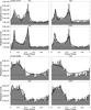 |
Fig. C.5 Top: PSR J1044-5737; bottom: PSR J1135-6055. For each model the best γ-ray light-curve (thick black line) is superimposed on the LAT pulsar light-curve (shaded histogram). The estimated background is indicated by the dash-dot line. |
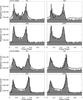 |
Fig. C.6 Top: PSR J1413-6205; bottom: PSR J1418-6058. For each model the best γ-ray light-curve (thick black line) is superimposed on the LAT pulsar light-curve (shaded histogram). The estimated background is indicated by the dash-dot line. |
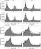 |
Fig. C.7 Top: PSR J1429-5911; bottom: PSR J1459-6053. For each model the best γ-ray light-curve (thick black line) is superimposed on the LAT pulsar light-curve (shaded histogram). The estimated background is indicated by the dash-dot line. |
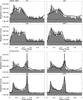 |
Fig. C.8 Top: PSR J1620-4927; bottom: PSR J1732-3131. For each model the best γ-ray light-curve (thick black line) is superimposed on the LAT pulsar light-curve (shaded histogram). The estimated background is indicated by the dash-dot line. |
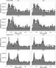 |
Fig. C.9 Top: PSR J1746-3239; bottom: PSR J1803-2149. For each model the best γ-ray light-curve (thick black line) is superimposed on the LAT pulsar light-curve (shaded histogram). The estimated background is indicated by the dash-dot line. |
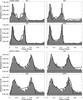 |
Fig. C.10 Top: PSR J1809-2332; bottom: PSR J1813-1246. For each model the best γ-ray light-curve (thick black line) is superimposed on the LAT pulsar light-curve (shaded histogram). The estimated background is indicated by the dash-dot line. |
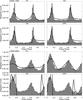 |
Fig. C.11 Top: PSR J1826-1256; bottom: PSR J1836+5925. For each model the best γ-ray light-curve (thick black line) is superimposed on the LAT pulsar light-curve (shaded histogram). The estimated background is indicated by the dash-dot line. For PSR J1836+5925 the SG is the only model that predicts enough off-pulse emission while OG and OPC models completely fail in explaining the observation probably because they do not predict enough off-pulse emission. |
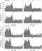 |
Fig. C.12 Top: PSR J1838-0537; bottom: PSR J1846+0919. For each model the best γ-ray light-curve (thick black line) is superimposed on the LAT pulsar light-curve (shaded histogram). The estimated background is indicated by the dash-dot line. |
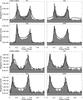 |
Fig. C.13 Top: PSR J1907+0602; bottom: PSR J1954+2836. For each model the best γ-ray light-curve (thick black line) is superimposed on the LAT pulsar light-curve (shaded histogram). The estimated background is indicated by the dash-dot line. |
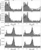 |
Fig. C.14 Top: PSR J1957+5033; bottom: PSR J1958+2846. For each model the best γ-ray light-curve (thick black line) is superimposed on the LAT pulsar light-curve (shaded histogram). The estimated background is indicated by the dash-dot line. |
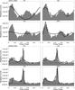 |
Fig. C.15 Top: PSR J2021+4026; bottom: PSR J2028+3332. For each model the best γ-ray light-curve (thick black line) is superimposed on the LAT pulsar light-curve (shaded histogram). The estimated background is indicated by the dash-dot line. |
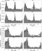 |
Fig. C.16 Top: PSR J2030+4415; bottom: PSR J2055+2539. For each model the best γ-ray light-curve (thick black line) is superimposed on the LAT pulsar light-curve (shaded histogram). The estimated background is indicated by the dash-dot line. |
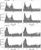 |
Fig. C.17 Top: PSR J2111+4606; bottom: PSR J2139+4716. For each model the best γ-ray light-curve (thick black line) is superimposed on the LAT pulsar light-curve (shaded histogram). The estimated background is indicated by the dash-dot line. |
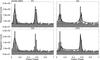 |
Fig. C.18 PSR J2238+5903. For each model the best γ-ray light-curve (thick black line) is superimposed on the LAT pulsar light-curve (shaded histogram). The estimated background is indicated by the dash-dot line. |
Appendix D: The LAT pulsar Joint fit light-curve results
Best fit log-likelihood values resulting from the γ-ray fit of the 41 RL pulsars of the analysed sample.
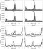 |
Fig. D.1 PSR J0205+6449. Top: for each model the best joint fit solution γ-ray light-curve (thick black line) is superimposed on the LAT pulsar γ-ray light-curve (shaded histogram). The estimated background is indicated by the dash-dot line. Bottom: for each model the best joint fit solution radio light-curve (black line) is superimposed on the LAT pulsar radio light-curve (grey thick line). The radio model is unique, but the (α,ζ) solutions vary for each γ-ray model. |
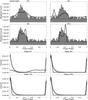 |
Fig. D.2 PSR J0248+6021. Top: for each model the best joint fit solution γ-ray light-curve (thick black line) is superimposed on the LAT pulsar γ-ray light-curve (shaded histogram). The estimated background is indicated by the dash-dot line. Bottom: for each model the best joint fit solution radio light-curve (black line) is superimposed on the LAT pulsar radio light-curve (grey thick line). The radio model is unique, but the (α,ζ) solutions vary for each γ-ray model. |
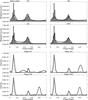 |
Fig. D.3 PSR J0534+2200. Top: for each model the best joint fit solution γ-ray light-curve (thick black line) is superimposed on the LAT pulsar γ-ray light-curve (shaded histogram). The estimated background is indicated by the dash-dot line. Bottom: for each model the best joint fit solution radio light-curve (black line) is superimposed on the LAT pulsar radio light-curve (grey thick line). The radio model is unique, but the (α,ζ) solutions vary for each γ-ray model. See Sect. 2 for a discussion on why we decided to show the joint γ-ray plus Radio fit result for the Crab pulsar. |
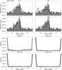 |
Fig. D.4 PSR J0631+1036. Top: for each model the best joint fit solution γ-ray light-curve (thick black line) is superimposed on the LAT pulsar γ-ray light-curve (shaded histogram). The estimated background is indicated by the dash-dot line. Bottom: for each model the best joint fit solution radio light-curve (black line) is superimposed on the LAT pulsar radio light-curve (grey thick line). The radio model is unique, but the (α,ζ) solutions vary for each γ-ray model. |
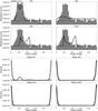 |
Fig. D.5 PSR J0659+1414. Top: for each model the best joint fit solution γ-ray light-curve (thick black line) is superimposed on the LAT pulsar γ-ray light-curve (shaded histogram). The estimated background is indicated by the dash-dot line. Bottom: for each model the best joint fit solution radio light-curve (black line) is superimposed on the LAT pulsar radio light-curve (grey thick line). The radio model is unique, but the (α,ζ) solutions vary for each γ-ray model. |
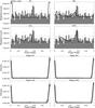 |
Fig. D.6 PSR J0729-1448. Top: for each model the best joint fit solution γ-ray light-curve (thick black line) is superimposed on the LAT pulsar γ-ray light-curve (shaded histogram). The estimated background is indicated by the dash-dot line. Bottom: for each model the best joint fit solution radio light-curve (black line) is superimposed on the LAT pulsar radio light-curve (grey thick line). The radio model is unique, but the (α,ζ) solutions vary for each γ-ray model. |
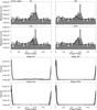 |
Fig. D.7 PSR J0742-2822. Top: for each model the best joint fit solution γ-ray light-curve (thick black line) is superimposed on the LAT pulsar γ-ray light-curve (shaded histogram). The estimated background is indicated by the dash-dot line. Bottom: for each model the best joint fit solution radio light-curve (black line) is superimposed on the LAT pulsar radio light-curve (grey thick line). The radio model is unique, but the (α,ζ) solutions vary for each γ-ray model. |
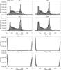 |
Fig. D.8 PSR J0835-4510. Top: for each model the best joint fit solution γ-ray light-curve (thick black line) is superimposed on the LAT pulsar γ-ray light-curve (shaded histogram). The estimated background is indicated by the dash-dot line. Bottom: for each model the best joint fit solution radio light-curve (black line) is superimposed on the LAT pulsar radio light-curve (grey thick line). The radio model is unique, but the (α,ζ) solutions vary for each γ-ray model. |
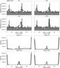 |
Fig. D.9 PSR J0908-4913. Top: for each model the best joint fit solution γ-ray light-curve (thick black line) is superimposed on the LAT pulsar γ-ray light-curve (shaded histogram). The estimated background is indicated by the dash-dot line. Bottom: for each model the best joint fit solution radio light-curve (black line) is superimposed on the LAT pulsar radio light-curve (grey thick line). The radio model is unique, but the (α,ζ) solutions vary for each γ-ray model. |
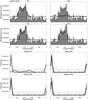 |
Fig. D.10 PSR J0940-5428. Top: for each model the best joint fit solution γ-ray light-curve (thick black line) is superimposed on the LAT pulsar γ-ray light-curve (shaded histogram). The estimated background is indicated by the dash-dot line. Bottom: for each model the best joint fit solution radio light-curve (black line) is superimposed on the LAT pulsar radio light-curve (grey thick line). The radio model is unique, but the (α,ζ) solutions vary for each γ-ray model. |
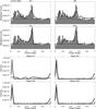 |
Fig. D.11 PSR J1016-5857. Top: for each model the best joint fit solution γ-ray light-curve (thick black line) is superimposed on the LAT pulsar γ-ray light-curve (shaded histogram). The estimated background is indicated by the dash-dot line. Bottom: for each model the best joint fit solution radio light-curve (black line) is superimposed on the LAT pulsar radio light-curve (grey thick line). The radio model is unique, but the (α,ζ) solutions vary for each γ-ray model. |
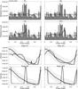 |
Fig. D.12 PSR J1019-5749. Top: for each model the best joint fit solution γ-ray light-curve (thick black line) is superimposed on the LAT pulsar γ-ray light-curve (shaded histogram). The estimated background is indicated by the dash-dot line. Bottom: for each model the best joint fit solution radio light-curve (black line) is superimposed on the LAT pulsar radio light-curve (grey thick line). The radio model is unique, but the (α,ζ) solutions vary for each γ-ray model. Because of the low statistics of the γ-ray light curve, the best-fit solution of each model is dominated by the radio light curve. The optimum-solution is given by the SG model but it represents an unreliable result since the best fit γ-ray light curve corresponds to a flat profile. |
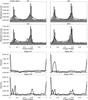 |
Fig. D.13 PSR J1028-5819. Top: for each model the best joint fit solution γ-ray light-curve (thick black line) is superimposed on the LAT pulsar γ-ray light-curve (shaded histogram). The estimated background is indicated by the dash-dot line. Bottom: for each model the best joint fit solution radio light-curve (black line) is superimposed on the LAT pulsar radio light-curve (grey thick line). The radio model is unique, but the (α,ζ) solutions vary for each γ-ray model. |
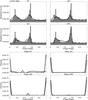 |
Fig. D.14 PSR J1048-5832. Top: for each model the best joint fit solution γ-ray light-curve (thick black line) is superimposed on the LAT pulsar γ-ray light-curve (shaded histogram). The estimated background is indicated by the dash-dot line. Bottom: for each model the best joint fit solution radio light-curve (black line) is superimposed on the LAT pulsar radio light-curve (grey thick line). The radio model is unique, but the (α,ζ) solutions vary for each γ-ray model. |
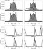 |
Fig. D.15 PSR J1057-5226. Top: for each model the best joint fit solution γ-ray light-curve (thick black line) is superimposed on the LAT pulsar γ-ray light-curve (shaded histogram). The estimated background is indicated by the dash-dot line. Bottom: for each model the best joint fit solution radio light-curve (black line) is superimposed on the LAT pulsar radio light-curve (grey thick line). The radio model is unique, but the (α,ζ) solutions vary for each γ-ray model. |
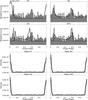 |
Fig. D.16 PSR J1105-6107. Top: for each model the best joint fit solution γ-ray light-curve (thick black line) is superimposed on the LAT pulsar γ-ray light-curve (shaded histogram). The estimated background is indicated by the dash-dot line. Bottom: for each model the best joint fit solution radio light-curve (black line) is superimposed on the LAT pulsar radio light-curve (grey thick line). The radio model is unique, but the (α,ζ) solutions vary for each γ-ray model. |
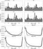 |
Fig. D.17 PSR J1112-6103. Top: for each model the best joint fit solution γ-ray light-curve (thick black line) is superimposed on the LAT pulsar γ-ray light-curve (shaded histogram). The estimated background is indicated by the dash-dot line. Bottom: for each model the best joint fit solution radio light-curve (black line) is superimposed on the LAT pulsar radio light-curve (grey thick line). The radio model is unique, but the (α,ζ) solutions vary for each γ-ray model. |
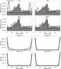 |
Fig. D.18 PSR J1119-6127. Top: for each model the best joint fit solution γ-ray light-curve (thick black line) is superimposed on the LAT pulsar γ-ray light-curve (shaded histogram). The estimated background is indicated by the dash-dot line. Bottom: for each model the best joint fit solution radio light-curve (black line) is superimposed on the LAT pulsar radio light-curve (grey thick line). The radio model is unique, but the (α,ζ) solutions vary for each γ-ray model. |
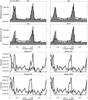 |
Fig. D.19 PSR J1124-5916. Top: for each model the best joint fit solution γ-ray light-curve (thick black line) is superimposed on the LAT pulsar γ-ray light-curve (shaded histogram). The estimated background is indicated by the dash-dot line. Bottom: for each model the best joint fit solution radio light-curve (black line) is superimposed on the LAT pulsar radio light-curve (grey thick line). The radio model is unique, but the (α,ζ) solutions vary for each γ-ray model. |
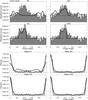 |
Fig. D.20 PSR J1357-6429. Top: for each model the best joint fit solution γ-ray light-curve (thick black line) is superimposed on the LAT pulsar γ-ray light-curve (shaded histogram). The estimated background is indicated by the dash-dot line. Bottom: for each model the best joint fit solution radio light-curve (black line) is superimposed on the LAT pulsar radio light-curve (grey thick line). The radio model is unique, but the (α,ζ) solutions vary for each γ-ray model. |
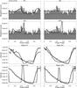 |
Fig. D.21 PSR J1410-6132. Top: for each model the best joint fit solution γ-ray light-curve (thick black line) is superimposed on the LAT pulsar γ-ray light-curve (shaded histogram). The estimated background is indicated by the dash-dot line. Bottom: for each model the best joint fit solution radio light-curve (black line) is superimposed on the LAT pulsar radio light-curve (grey thick line). The radio model is unique, but the (α,ζ) solutions vary for each γ-ray model. For this pulsar the SG model gives the optimum-solution but it represents an unreliable result since the best fit γ-ray light curve correspond to a flat profile. |
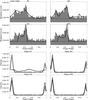 |
Fig. D.22 PSR J1420-6048. Top: for each model the best joint fit solution γ-ray light-curve (thick black line) is superimposed on the LAT pulsar γ-ray light-curve (shaded histogram). The estimated background is indicated by the dash-dot line. Bottom: for each model the best joint fit solution radio light-curve (black line) is superimposed on the LAT pulsar radio light-curve (grey thick line). The radio model is unique, but the (α,ζ) solutions vary for each γ-ray model. |
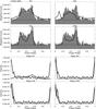 |
Fig. D.23 PSR J1509-5850. Top: for each model the best joint fit solution γ-ray light-curve (thick black line) is superimposed on the LAT pulsar γ-ray light-curve (shaded histogram). The estimated background is indicated by the dash-dot line. Bottom: for each model the best joint fit solution radio light-curve (black line) is superimposed on the LAT pulsar radio light-curve (grey thick line). The radio model is unique, but the (α,ζ) solutions vary for each γ-ray model. |
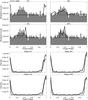 |
Fig. D.24 PSR J1513-5908. Top: for each model the best joint fit solution γ-ray light-curve (thick black line) is superimposed on the LAT pulsar γ-ray light-curve (shaded histogram). The estimated background is indicated by the dash-dot line. Bottom: for each model the best joint fit solution radio light-curve (black line) is superimposed on the LAT pulsar radio light-curve (grey thick line). The radio model is unique, but the (α,ζ) solutions vary for each γ-ray model. |
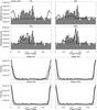 |
Fig. D.25 PSR J1648-4611. Top: for each model the best joint fit solution γ-ray light-curve (thick black line) is superimposed on the LAT pulsar γ-ray light-curve (shaded histogram). The estimated background is indicated by the dash-dot line. Bottom: for each model the best joint fit solution radio light-curve (black line) is superimposed on the LAT pulsar radio light-curve (grey thick line). The radio model is unique, but the (α,ζ) solutions vary for each γ-ray model. |
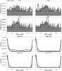 |
Fig. D.26 PSR J1702-4128. Top: for each model the best joint fit solution γ-ray light-curve (thick black line) is superimposed on the LAT pulsar γ-ray light-curve (shaded histogram). The estimated background is indicated by the dash-dot line. Bottom: for each model the best joint fit solution radio light-curve (black line) is superimposed on the LAT pulsar radio light-curve (grey thick line). The radio model is unique, but the (α,ζ) solutions vary for each γ-ray model. |
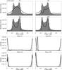 |
Fig. D.27 PSR J1709-4429. Top: for each model the best joint fit solution γ-ray light-curve (thick black line) is superimposed on the LAT pulsar γ-ray light-curve (shaded histogram). The estimated background is indicated by the dash-dot line. Bottom: for each model the best joint fit solution radio light-curve (black line) is superimposed on the LAT pulsar radio light-curve (grey thick line). The radio model is unique, but the (α,ζ) solutions vary for each γ-ray model. |
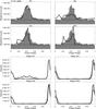 |
Fig. D.28 PSR J1718-3825. Top: for each model the best joint fit solution γ-ray light-curve (thick black line) is superimposed on the LAT pulsar γ-ray light-curve (shaded histogram). The estimated background is indicated by the dash-dot line. Bottom: for each model the best joint fit solution radio light-curve (black line) is superimposed on the LAT pulsar radio light-curve (grey thick line). The radio model is unique, but the (α,ζ) solutions vary for each γ-ray model. |
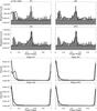 |
Fig. D.29 PSR J1730-3350. Top: for each model the best joint fit solution γ-ray light-curve (thick black line) is superimposed on the LAT pulsar γ-ray light-curve (shaded histogram). The estimated background is indicated by the dash-dot line. Bottom: for each model the best joint fit solution radio light-curve (black line) is superimposed on the LAT pulsar radio light-curve (grey thick line). The radio model is unique, but the (α,ζ) solutions vary for each γ-ray model. |
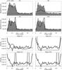 |
Fig. D.30 PSR J1741-2054. Top: for each model the best joint fit solution γ-ray light-curve (thick black line) is superimposed on the LAT pulsar γ-ray light-curve (shaded histogram). The estimated background is indicated by the dash-dot line. Bottom: for each model the best joint fit solution radio light-curve (black line) is superimposed on the LAT pulsar radio light-curve (grey thick line). The radio model is unique, but the (α,ζ) solutions vary for each γ-ray model. |
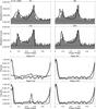 |
Fig. D.31 PSR J1747-2958. Top: for each model the best joint fit solution γ-ray light-curve (thick black line) is superimposed on the LAT pulsar γ-ray light-curve (shaded histogram). The estimated background is indicated by the dash-dot line. Bottom: for each model the best joint fit solution radio light-curve (black line) is superimposed on the LAT pulsar radio light-curve (grey thick line). The radio model is unique, but the (α,ζ) solutions vary for each γ-ray model. |
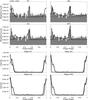 |
Fig. D.32 PSR J1801-2451. Top: for each model the best joint fit solution γ-ray light-curve (thick black line) is superimposed on the LAT pulsar γ-ray light-curve (shaded histogram). The estimated background is indicated by the dash-dot line. Bottom: for each model the best joint fit solution radio light-curve (black line) is superimposed on the LAT pulsar radio light-curve (grey thick line). The radio model is unique, but the (α,ζ) solutions vary for each γ-ray model. |
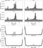 |
Fig. D.33 PSR J1833-1034. Top: for each model the best joint fit solution γ-ray light-curve (thick black line) is superimposed on the LAT pulsar γ-ray light-curve (shaded histogram). The estimated background is indicated by the dash-dot line. Bottom: for each model the best joint fit solution radio light-curve (black line) is superimposed on the LAT pulsar radio light-curve (grey thick line). The radio model is unique, but the (α,ζ) solutions vary for each γ-ray model. |
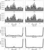 |
Fig. D.34 PSR J1835-1106. Top: for each model the best joint fit solution γ-ray light-curve (thick black line) is superimposed on the LAT pulsar γ-ray light-curve (shaded histogram). The estimated background is indicated by the dash-dot line. Bottom: for each model the best joint fit solution radio light-curve (black line) is superimposed on the LAT pulsar radio light-curve (grey thick line). The radio model is unique, but the (α,ζ) solutions vary for each γ-ray model. |
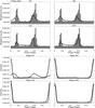 |
Fig. D.35 PSR J1952+3252. Top: for each model the best joint fit solution γ-ray light-curve (thick black line) is superimposed on the LAT pulsar γ-ray light-curve (shaded histogram). The estimated background is indicated by the dash-dot line. Bottom: for each model the best joint fit solution radio light-curve (black line) is superimposed on the LAT pulsar radio light-curve (grey thick line). The radio model is unique, but the (α,ζ) solutions vary for each γ-ray model. |
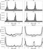 |
Fig. D.36 PSR J2021+3651. Top: for each model the best joint fit solution γ-ray light-curve (thick black line) is superimposed on the LAT pulsar γ-ray light-curve (shaded histogram). The estimated background is indicated by the dash-dot line. Bottom: for each model the best joint fit solution radio light-curve (black line) is superimposed on the LAT pulsar radio light-curve (grey thick line). The radio model is unique, but the (α,ζ) solutions vary for each γ-ray model. |
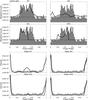 |
Fig. D.37 PSR J2030+3641. Top: for each model the best joint fit solution γ-ray light-curve (thick black line) is superimposed on the LAT pulsar γ-ray light-curve (shaded histogram). The estimated background is indicated by the dash-dot line. Bottom: for each model the best joint fit solution radio light-curve (black line) is superimposed on the LAT pulsar radio light-curve (grey thick line). The radio model is unique, but the (α,ζ) solutions vary for each γ-ray model. |
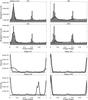 |
Fig. D.38 PSR J2032+4127. Top: for each model the best joint fit solution γ-ray light-curve (thick black line) is superimposed on the LAT pulsar γ-ray light-curve (shaded histogram). The estimated background is indicated by the dash-dot line. Bottom: for each model the best joint fit solution radio light-curve (black line) is superimposed on the LAT pulsar radio light-curve (grey thick line). The radio model is unique, but the (α,ζ) solutions vary for each γ-ray model. |
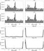 |
Fig. D.39 PSR J2043+2740. Top: for each model the best joint fit solution γ-ray light-curve (thick black line) is superimposed on the LAT pulsar γ-ray light-curve (shaded histogram). The estimated background is indicated by the dash-dot line. Bottom: for each model the best joint fit solution radio light-curve (black line) is superimposed on the LAT pulsar radio light-curve (grey thick line). The radio model is unique, but the (α,ζ) solutions vary for each γ-ray model. |
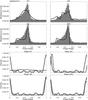 |
Fig. D.40 PSR J2229+6114. Top: for each model the best joint fit solution γ-ray light-curve (thick black line) is superimposed on the LAT pulsar γ-ray light-curve (shaded histogram). The estimated background is indicated by the dash-dot line. Bottom: for each model the best joint fit solution radio light-curve (black line) is superimposed on the LAT pulsar radio light-curve (grey thick line). The radio model is unique, but the (α,ζ) solutions vary for each γ-ray model. |
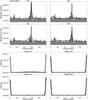 |
Fig. D.41 PSR J2240+5832. Top: for each model the best joint fit solution γ-ray light-curve (thick black line) is superimposed on the LAT pulsar γ-ray light-curve (shaded histogram). The estimated background is indicated by the dash-dot line. Bottom: for each model the best joint fit solution radio light-curve (black line) is superimposed on the LAT pulsar radio light-curve (grey thick line). The radio model is unique, but the (α,ζ) solutions vary for each γ-ray model. |
Appendix E: Joint fit of radio and γ-ray light curves of the radio-faint pulsars J0106+4855 and J1907+0602
In this Appendix we give the results of the joint-fit of radio and γ-ray light curve for the 2 RF pulsars J0106+4855 and J1907+0602.
Appendix E.1: J0106+4855
Figure E.1 shows the best-fit radio and γ-ray light curves for pulsar J0106+4855 while its best joint-fit parameters are given in Table E.1. The PC joint-fit solution is characterised by lower α and ζ angles and similar | α − ζ | and fΩ values when compared with the γ-ray only fit solution, while the SG model joint-fit solution is overall consistent with the γ-ray-only fit results. For OG and OPC models, the joint-fit α values are larger than the values obtained through γ-ray only fit. This implies a lower joint-fit | α − ζ | value that favours simultaneous γ-ray and radio emission. Moreover the OG and OPC joint-fit values of fΩ are larger than the values obtained with the γ-ray only fit and this favours the overlapping of γ-ray and radio beam to give a RL pulsar.
Concerning the best fit radio and γ-ray light curves, the largest PC likelihood value shown in Table E.1 is fictitious since the PC γ-ray fit shown in Fig. E.1 explains just one of the two γ-ray peaks. In agreement with the γ-ray only fit that predicts a two peaks γ-ray light curve just for PC and SG models (Fig. C.1), the SG is the model that best explains simultaneous γ-ray and radio emission from pulsar J0106+4855.
Appendix E.2: J1907+0602
Figure E.2 shows the best-fit radio and γ-ray light curves for pulsar J1907+0602 while its best joint-fit parameters are given in Table E.2. Both PC and SG model best joint-fit parameters are consistent with the γ-ray-only fit results. As for pulsar J0106+4855, the OG and OPC models best-fit results predict α values larger than the values obtained through γ-ray only fit and larger values of fΩ. The lower | α − ζ | joint-fit values and the larger fΩ joint-fit values favour the overlapping of γ-ray and radio beam to give a RL pulsar.
In agreement with the γ-ray only fit that predicts a γ-ray light curves with two peaks connected by a high bridge just for OG and OPC models (Fig. C.13), the OG is the model that best explains simultaneous γ-ray and radio emission from pulsar J1907+0602.
Best fit parameters resulting from the joint fit of radio and γ-ray light curves of pulsar J0106+4855.
Best fit parameters resulting from the joint fit of radio and γ-ray light curves of pulsar J1907+0602.
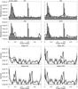 |
Fig. E.1 PSR J0106+4855. Top: for each model the best joint fit solution γ-ray light-curve (thick black line) is superimposed on the LAT pulsar γ-ray light-curve (shaded histogram). The estimated background is indicated by the dash-dot line. Bottom: for each model the best joint fit solution radio light-curve (black line) is superimposed on the LAT pulsar radio light-curve (grey thick line). The radio model is unique, but the (α,ζ) solutions vary for each γ-ray model. |
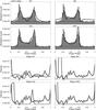 |
Fig. E.2 PSR J1907+0602. Top: for each model the best joint fit solution γ-ray light-curve (thick black line) is superimposed on the LAT pulsar γ-ray light-curve (shaded histogram). The estimated background is indicated by the dash-dot line. Bottom: for each model the best joint fit solution radio light-curve (black line) is superimposed on the LAT pulsar radio light-curve (grey thick line). The radio model is unique, but the (α,ζ) solutions vary for each γ-ray model. |
Acknowledgments
The Fermi LAT Collaboration acknowledges generous ongoing support from a number of agencies and institutes that have supported both the development and the operation of the LAT as well as scientific data analysis. These include the National Aeronautics and Space Administration and the Department of Energy in the United States, the Commissariat à l’Énergie Atomique and the Centre National de la Recherche Scientifique/Institut National de Physique Nucléaire et de Physique des Particules in France, the Agenzia Spaziale Italiana and the Istituto Nazionale di Fisica Nucleare in Italy, the Ministry of Education, Culture, Sports, Science and Technology (MEXT), High Energy Accelerator Research Organization (KEK) and Japan Aerospace Exploration Agency (JAXA) in Japan, and the K. A. Wallenberg Foundation, the Swedish Research Council and the Swedish National Space Board in Sweden. Additional support for science analysis during the operations phase is gratefully acknowledged from the Istituto Nazionale di Astrofisica in Italy and the Centre National d’Études Spatiales in France. M.P. acknowledges IASF-INAF in Milan for fundamental support during the realisation of this project, the Nicolaus Copernicus Astronomical Center, grant DEC-2011/02/A/ST9/00256, for providing software and computer facilities needed for the conclusion of this work, and Sacha Hony for the precious help. And a very special thanks to Isabel Caballero, Isa, for supporting me so many years, for teaching me many things, and for being there with me in daily life. A.K.H. acknowledges support from the NASA Astrophysics Theory and Fermi GI Programs. The authors wish to acknowledge the anonymous referee for the helpful suggestions and comments that enriched the paper and helped to highlight some of its results. The authors gratefullys acknowledge the Pulsar Search and Timing Consortia, all the radio scientists who contributed in providing the radio light curves used in this paper, and the radio observatories that generated the radio profiles used in this paper: the Parkes Radio Telescope is part of the Australia Telescope which is funded by the Commonwealth Government for operation as a National Facility managed by CSIRO; the Green Bank Telescope is operated by the National Radio Astronomy Observatory, a facility of the National Science Foundation operated under cooperative agreement by Associated Universities, Inc; the Arecibo Observatory is part of the National Astronomy and Ionosphere Center (NAIC), a national research center operated by Cornell University under a cooperative agreement with the National Science Foundation; the Nançay Radio Observatory is operated by the Paris Observatory, associated with the French Centre National de la Recherche Scientifique (CNRS); the Lovell Telescope is owned and operated by the University of Manchester as part of the Jodrell Bank Centre for Astrophysics with support from the Science and Technology Facilities Council of the United Kingdom; the Westerbork Synthesis Radio Telescope is operated by Netherlands Foundation for Radio Astronomy, ASTRON.
References
- Abdo, A. A., Ackermann, M., Ajello, M., et al. 2010a, ApJ, 713, 154 [NASA ADS] [CrossRef] [Google Scholar]
- Abdo, A. A., Ackermann, M., Ajello, M., et al. 2010b, ApJ, 187, 460 [Google Scholar]
- Abdo, A. A., Ajello, M., Allafort, A., et al. 2013, ApJS, 208, 17 [NASA ADS] [CrossRef] [Google Scholar]
- Arons, J. 1983, ApJ, 266, 215 [NASA ADS] [CrossRef] [Google Scholar]
- Atwood, W. B., Abdo, A. A., Ackermann, M., et al. 2009, ApJ, 697, 1071 [NASA ADS] [CrossRef] [Google Scholar]
- Bai, X.-N., & Spitkovsky, A. 2010, ApJ, 715, 1270 [NASA ADS] [CrossRef] [Google Scholar]
- Caraveo, P. A., Bignami, G. F., DeLuca, A., et al. 2003, Science, 301, 1345 [NASA ADS] [CrossRef] [Google Scholar]
- Cheng, K. S., Ho, C., & Ruderman, M. 1986, ApJ, 300, 500 [NASA ADS] [CrossRef] [Google Scholar]
- Cheng, K. S., Ruderman, M., & Zhang, L. 2000, ApJ, 537, 964 [NASA ADS] [CrossRef] [Google Scholar]
- Deutsch, A. J. 1955, Ann. Astrophys., 18, 1 [NASA ADS] [Google Scholar]
- Dyks, J., & Rudak, B. 2003, ApJ, 598, 1201 [NASA ADS] [CrossRef] [Google Scholar]
- Dyks, J., Harding, A. K., & Rudak, B. 2004, ApJ, 606, 1125 [NASA ADS] [CrossRef] [Google Scholar]
- Goldreich, P., & Julian, W. H. 1969, ApJ, 157, 869 [NASA ADS] [CrossRef] [Google Scholar]
- Gonthier, P. L., Van Guilder, R., Harding, A. K., Greneir, I., & Perrot, C. 2004, BAAS, 36, 918 [NASA ADS] [Google Scholar]
- Harding, A. K., & Muslimov, A. G. 2011, ApJ, 726, L10 [NASA ADS] [CrossRef] [Google Scholar]
- Harding, A. K., Grenier, I. A., & Gonthier, P. L. 2007, Ap&SS, 309, 221 [NASA ADS] [CrossRef] [Google Scholar]
- Hobbs, G., Edwards, R., & Manchester, R. 2006, Chin. J. Astron. Astrophys., 6, 189 [Google Scholar]
- Johnson, T. J., Venter, C., Harding, A. K., & Guillemot, L. 2011, in AIP Conf. Ser. 1357, eds. M. Burgay, N. D’Amico, P. Esposito, A. Pellizzoni, & A. Possenti, 237 [Google Scholar]
- Johnston, S., Hobbs, G., Vigeland, S., et al. 2005, MNRAS, 364, 1397 [NASA ADS] [CrossRef] [Google Scholar]
- Jones, P. B. 1976, Ap&SS, 45, 369 [NASA ADS] [CrossRef] [Google Scholar]
- Kalapotharakos, C., Harding, A. K., & Kazanas, D. 2014, ApJ, 793, 97 [NASA ADS] [CrossRef] [Google Scholar]
- Kerr, M. 2011, ApJ, 732, 38 [NASA ADS] [CrossRef] [Google Scholar]
- Manchester, R. N. 2005, Ap&SS, 297, 101 [NASA ADS] [CrossRef] [Google Scholar]
- McBreen, B., Ball, Jr., S. E., Campbell, M., Greisen, K., & Koch, D. 1973, ApJ, 184, 571 [NASA ADS] [CrossRef] [Google Scholar]
- Muslimov, A. G., & Harding, A. K. 2003, ApJ, 588, 430 [NASA ADS] [CrossRef] [Google Scholar]
- Muslimov, A. G., & Harding, A. K. 2004, ApJ, 606, 1143 [NASA ADS] [CrossRef] [Google Scholar]
- Ng, C., & Romani, R. W. 2008, ApJ, 673, 411 [NASA ADS] [CrossRef] [Google Scholar]
- Pierbattista, M. 2010, Ph.D. Thesis, Université Paris 7 Denis Diderot [arXiv:1309.5982] [Google Scholar]
- Pierbattista, M., Grenier, I. A., Harding, A. K., & Gonthier, P. L. 2012, A&A, 545, A42 [NASA ADS] [CrossRef] [EDP Sciences] [Google Scholar]
- Ravi, V., Wyithe, J. S. B., Hobbs, G., et al. 2012, ApJ, 761, 84 [NASA ADS] [CrossRef] [Google Scholar]
- Ray, P. S., Kerr, M., Parent, D., et al. 2011, ApJS, 194, 17 [NASA ADS] [CrossRef] [Google Scholar]
- Ray, P. S., Abdo, A. A., Parent, D., et al. 2012, 2011 Fermi Symp. Proc., eConf C110509 [arXiv:1205.3089] [Google Scholar]
- Romani, R. W., & Watters, K. P. 2010, ApJ, 714, 810 [NASA ADS] [CrossRef] [Google Scholar]
- Smith, D. A., Guillemot, L., Camilo, F., et al. 2008, A&A, 492, 923 [NASA ADS] [CrossRef] [EDP Sciences] [Google Scholar]
- Story, S. A., Gonthier, P. L., & Harding, A. K. 2007, ApJ, 671, 713 [NASA ADS] [CrossRef] [Google Scholar]
- Sturrock, P. A. 1971, ApJ, 164, 529 [NASA ADS] [CrossRef] [Google Scholar]
- Takata, J., Wang, Y., & Cheng, K. S. 2011, ApJ, 726, 44 [NASA ADS] [CrossRef] [Google Scholar]
- Venter, C., Harding, A. K., & Guillemot, L. 2009, ApJ, 707, 800 [NASA ADS] [CrossRef] [Google Scholar]
- Venter, C., Johnson, T. J., & Harding, A. K. 2012, ApJ, 744, 34 [NASA ADS] [CrossRef] [Google Scholar]
- Watters, K. P., & Romani, R. W. 2011, ApJ, 727, 123 [NASA ADS] [CrossRef] [Google Scholar]
- Watters, K. P., Romani, R. W., Weltevrede, P., & Johnston, S. 2009, ApJ, 695, 1289 [NASA ADS] [CrossRef] [Google Scholar]
- Young, M. D. T., Chan, L. S., Burman, R. R., & Blair, D. G. 2010, MNRAS, 402, 1317 [NASA ADS] [CrossRef] [Google Scholar]
All Tables
α and ζ best-fit solutions resulting from the γ-ray fit of the 33 RQ plus 2 RF pulsars.
Estimate of the systematic errors on α and ζ obtained from the comparison of the FCBin and RBin fits.
α and ζ best-fit solutions resulting from the joint radio plus γ-ray fit of the 41 RL pulsars.
Estimate of the systematic errors on α and ζ obtained from the comparison of the two joint fit methods γ-ray fit plus σpeak radio fit and γ-ray fit plus σ∗ radio fit.
Left: for each model, the number (and frequency in the sample) of optimum-solutions that yield a better fit than the other models by at least 1σ. Right: for each model, the number and frequency of solutions that are rejected by more than 3σ compared to the optimum-model.
α and ζ best-fit solution resulting from the γ-ray only fit of the 41 RL pulsars.
Beaming factors fΩ evaluated for the RQ (left) and RL (right) pulsars in the framework of each model.
Best power-law fits to the distribution of fΩ and Lγ as functions of Ė for each model and RL or RQ pulsars.
Best power-law fits to the distribution of Ecut and Γ as functions of the width of the acceleration gap for each model and RL or RQ pulsars.
Best fit log-likelihood values resulting from the γ-ray fit of the 35 RQ pulsars of the analysed sample.
Best fit log-likelihood values resulting from the γ-ray fit of the 41 RL pulsars of the analysed sample.
Best fit parameters resulting from the joint fit of radio and γ-ray light curves of pulsar J0106+4855.
Best fit parameters resulting from the joint fit of radio and γ-ray light curves of pulsar J1907+0602.
All Figures
|
Fig. 1 Top left to bottom right panels: phase-plots obtained for the PC, SG, OG/OPC, and radio (core plus cone) models respectively, with a magnetic field strength of BG = 108 Tesla and spin period of 30 ms for the PC and radio cases, and gap widths of 0.04 and 0.01 for the SG and OG/OPC cases, respectively. All the plots are given for an obliquity α = 45°. The emission flux increases from black to red. |
| In the text | |
|
Fig. 2 α-ζ log-likelihood maps obtained by fitting the γ-ray light curve of pulsar J1023−5746 with each γ-ray model phase plot. The fit has been performed with χ2 estimator and FCBin light curves. A white circle shows the position of the best-fit solutions. The colour-bar is in effective σ = ( | lnL − lnLmax | )0.5 units, zero corresponds to the best-fit solution. The diagonal band present in the PC panel is due to the fact that the emission region is located close to the polar cap and shines mainly when ζobs ≅ α. Elsewhere, for | ζobs − α | >ρ/ 2 with ρ the opening angle of the PC emission cone, no PC emission is visible from the pulsars and the simulated light curves for those angles are fitted as flat background emission. This generates the observed yellow flat field in the log-likelihood map. |
| In the text | |
|
Fig. 3 Comparison of the relative goodness of the fit solutions obtained for the RQ LAT pulsars between the optimum-model and alternative models. The comparison is expressed as the |
| In the text | |
|
Fig. 4 For each model the (α,ζ) log-likelihood map for the γ-ray fit, the radio fit, and the sum of these two maps for pulsar J0205+6449 is shown. A white circle shows the position of the best fit solution for each log-likelihood map. The colour-bar is in effective σ = ( | lnL − lnLmax | )0.5 units, zero corresponds to the best-fit solution. |
| In the text | |
|
Fig. 5 Comparison of the relative goodness of the fit solutions obtained for the RL LAT pulsars between the optimum-model and alternative models. The comparison is expressed as the |
| In the text | |
|
Fig. 6 Distribution of the α-ζ best-fit solutions obtained, for the RL pulsars sample and in the framework of each model, by fitting the γ-ray light curves alone (stars) and by jointly fitting the γ-ray and the radio light curves (squares). Recall that filled and empty symbols refer to the solutions of the optimum and alternative models, respectively. |
| In the text | |
|
Fig. 7 α-ζ plane distribution of RQ (top panel) and RL (bottom panel) fit solutions for the PC (magenta triangles), SG (red circles), OG (blue squares), and OPC (black stars) models. Recall that filled and empty symbols refer to best-fit solutions of the optimum and alternative models, respectively. The optimum-solutions that are better than the other models by more than 1σ are plotted as light-colour-filled symbols. |
| In the text | |
|
Fig. 8 Beaming factor fΩ versus the pulsar spin-down power Ė evaluated for RQ (top panel) and RL (bottom panel) pulsars . The lines represent the best power-law fits to the data points; the best fit power-law parameters with relative 1σ errors, are listed in Table 8. Hereafter the optimum-solutions that are better than the other models by more than 1σ will be plotted as light-colour-filled hexagrams. |
| In the text | |
|
Fig. 9 Beaming factor fΩ distribution for the RQ (top panel) and RL (bottom panel) pulsars and all models. |
| In the text | |
|
Fig. 10 γ-ray luminosity versus Ė for RQ (top panel) and RL (bottom panel) Fermi pulsars. The thick lines represent the best power-law fits to the data points; their parameters and 1σ errors are listed in Table 8. The thin dot-dashed line indicates 100% conversion of Ė into γ-rays. |
| In the text | |
|
Fig. 11 Geometric γ-ray luminosity, Lgeo versus the standard gap-model γ-ray luminosity Lrad for RQ (top panel) and RL (bottom panel) Fermi pulsars and each model. The dot-dashed lines indicates Lgeo = Lrad. |
| In the text | |
|
Fig. 12 Magnetic obliquity α versus characteristic age for RQ (top panel) and RL (bottom panel) Fermi pulsars and each model. |
| In the text | |
|
Fig. 13 Gap width as a function of α for RQ (top panel) and RL (bottom panel) Fermi pulsars and each model. |
| In the text | |
|
Fig. 14 For each model the β = | α − ζ | angles a function of the spin period for RQ (top panel) and RL (bottom panel) Fermi pulsars is shown. |
| In the text | |
|
Fig. 15 Energy cutoff versus gap width for RQ (top panel) and RL (bottom panel) Fermi pulsars for each model. The best fit power law trends are given in each figure. PC and SG results are characterised by the same gap width wSG and have been plotted together. |
| In the text | |
|
Fig. 16 Spectral index versus gap width for RQ (top panel) and RL (bottom panel) Fermi pulsars for each model. The best fit power law trends are given in each figure. PC and SG results are characterised by the same gap width wSG and have been plotted together. |
| In the text | |
|
Fig. 17 Variation, in a force-free magnetosphere, of the ratio Goldreich-Julian charge density over the magnetic field, ρGJ/B, with the distance from the pulsar expressed in unit of the light-cylinder radius, r/RLC. |
| In the text | |
|
Fig. B.1 Number density of the visible γ-ray pulsars obtained for each model as a function of α and ζ in the population synthesis of Pierbattista et al. (2012). The linear grey scale saturates at 1.5 star/bin. The pink contours outline the density obtained for the radio-loud γ-ray sub-sample (at 5% and 50% of the maximum density). The insert gives the set of ζ values measured by Ng & Romani (2008) from the orientation of the wind torus seen in X rays (pink lines) and by Caraveo et al. (2003) from the orientation of the Geminga X-ray tails (green line). The separation in α in the insert is meaningless. |
| In the text | |
|
Fig. B.2 Number density of the visible γ-ray pulsars obtained for each model as a function of gap width and high-energy cutoff (left) and of gap width and spectral index (right). The linear grey scale saturates at 8 star/bin. The pink contours outline the density obtained for the radio-loud γ-ray sub-sample (at 5% and 50% of the maximum density). |
| In the text | |
|
Fig. C.1 Top: PSR J0007+7303; bottom: PSR J0106+4855. For each model the best γ-ray light-curve (thick black line) is superimposed on the LAT pulsar light-curve (shaded histogram). The estimated background is indicated by the dash-dot line. |
| In the text | |
|
Fig. C.2 Top: PSR J0357+3205; bottom: PSR J0622+3749. For each model the best γ-ray light-curve (thick black line) is superimposed on the LAT pulsar light-curve (shaded histogram). The estimated background is indicated by the dash-dot line. |
| In the text | |
|
Fig. C.3 Top: PSR J0633+0632; bottom: PSR J0633+1746. For each model the best γ-ray light-curve (thick black line) is superimposed on the LAT pulsar light-curve (shaded histogram). The estimated background is indicated by the dash-dot line. |
| In the text | |
|
Fig. C.4 Top: PSR J0734-1559; bottom: PSR J1023-5746. For each model the best γ-ray light-curve (thick black line) is superimposed on the LAT pulsar light-curve (shaded histogram). The estimated background is indicated by the dash-dot line. |
| In the text | |
|
Fig. C.5 Top: PSR J1044-5737; bottom: PSR J1135-6055. For each model the best γ-ray light-curve (thick black line) is superimposed on the LAT pulsar light-curve (shaded histogram). The estimated background is indicated by the dash-dot line. |
| In the text | |
|
Fig. C.6 Top: PSR J1413-6205; bottom: PSR J1418-6058. For each model the best γ-ray light-curve (thick black line) is superimposed on the LAT pulsar light-curve (shaded histogram). The estimated background is indicated by the dash-dot line. |
| In the text | |
|
Fig. C.7 Top: PSR J1429-5911; bottom: PSR J1459-6053. For each model the best γ-ray light-curve (thick black line) is superimposed on the LAT pulsar light-curve (shaded histogram). The estimated background is indicated by the dash-dot line. |
| In the text | |
|
Fig. C.8 Top: PSR J1620-4927; bottom: PSR J1732-3131. For each model the best γ-ray light-curve (thick black line) is superimposed on the LAT pulsar light-curve (shaded histogram). The estimated background is indicated by the dash-dot line. |
| In the text | |
|
Fig. C.9 Top: PSR J1746-3239; bottom: PSR J1803-2149. For each model the best γ-ray light-curve (thick black line) is superimposed on the LAT pulsar light-curve (shaded histogram). The estimated background is indicated by the dash-dot line. |
| In the text | |
|
Fig. C.10 Top: PSR J1809-2332; bottom: PSR J1813-1246. For each model the best γ-ray light-curve (thick black line) is superimposed on the LAT pulsar light-curve (shaded histogram). The estimated background is indicated by the dash-dot line. |
| In the text | |
|
Fig. C.11 Top: PSR J1826-1256; bottom: PSR J1836+5925. For each model the best γ-ray light-curve (thick black line) is superimposed on the LAT pulsar light-curve (shaded histogram). The estimated background is indicated by the dash-dot line. For PSR J1836+5925 the SG is the only model that predicts enough off-pulse emission while OG and OPC models completely fail in explaining the observation probably because they do not predict enough off-pulse emission. |
| In the text | |
|
Fig. C.12 Top: PSR J1838-0537; bottom: PSR J1846+0919. For each model the best γ-ray light-curve (thick black line) is superimposed on the LAT pulsar light-curve (shaded histogram). The estimated background is indicated by the dash-dot line. |
| In the text | |
|
Fig. C.13 Top: PSR J1907+0602; bottom: PSR J1954+2836. For each model the best γ-ray light-curve (thick black line) is superimposed on the LAT pulsar light-curve (shaded histogram). The estimated background is indicated by the dash-dot line. |
| In the text | |
|
Fig. C.14 Top: PSR J1957+5033; bottom: PSR J1958+2846. For each model the best γ-ray light-curve (thick black line) is superimposed on the LAT pulsar light-curve (shaded histogram). The estimated background is indicated by the dash-dot line. |
| In the text | |
|
Fig. C.15 Top: PSR J2021+4026; bottom: PSR J2028+3332. For each model the best γ-ray light-curve (thick black line) is superimposed on the LAT pulsar light-curve (shaded histogram). The estimated background is indicated by the dash-dot line. |
| In the text | |
|
Fig. C.16 Top: PSR J2030+4415; bottom: PSR J2055+2539. For each model the best γ-ray light-curve (thick black line) is superimposed on the LAT pulsar light-curve (shaded histogram). The estimated background is indicated by the dash-dot line. |
| In the text | |
|
Fig. C.17 Top: PSR J2111+4606; bottom: PSR J2139+4716. For each model the best γ-ray light-curve (thick black line) is superimposed on the LAT pulsar light-curve (shaded histogram). The estimated background is indicated by the dash-dot line. |
| In the text | |
|
Fig. C.18 PSR J2238+5903. For each model the best γ-ray light-curve (thick black line) is superimposed on the LAT pulsar light-curve (shaded histogram). The estimated background is indicated by the dash-dot line. |
| In the text | |
|
Fig. D.1 PSR J0205+6449. Top: for each model the best joint fit solution γ-ray light-curve (thick black line) is superimposed on the LAT pulsar γ-ray light-curve (shaded histogram). The estimated background is indicated by the dash-dot line. Bottom: for each model the best joint fit solution radio light-curve (black line) is superimposed on the LAT pulsar radio light-curve (grey thick line). The radio model is unique, but the (α,ζ) solutions vary for each γ-ray model. |
| In the text | |
|
Fig. D.2 PSR J0248+6021. Top: for each model the best joint fit solution γ-ray light-curve (thick black line) is superimposed on the LAT pulsar γ-ray light-curve (shaded histogram). The estimated background is indicated by the dash-dot line. Bottom: for each model the best joint fit solution radio light-curve (black line) is superimposed on the LAT pulsar radio light-curve (grey thick line). The radio model is unique, but the (α,ζ) solutions vary for each γ-ray model. |
| In the text | |
|
Fig. D.3 PSR J0534+2200. Top: for each model the best joint fit solution γ-ray light-curve (thick black line) is superimposed on the LAT pulsar γ-ray light-curve (shaded histogram). The estimated background is indicated by the dash-dot line. Bottom: for each model the best joint fit solution radio light-curve (black line) is superimposed on the LAT pulsar radio light-curve (grey thick line). The radio model is unique, but the (α,ζ) solutions vary for each γ-ray model. See Sect. 2 for a discussion on why we decided to show the joint γ-ray plus Radio fit result for the Crab pulsar. |
| In the text | |
|
Fig. D.4 PSR J0631+1036. Top: for each model the best joint fit solution γ-ray light-curve (thick black line) is superimposed on the LAT pulsar γ-ray light-curve (shaded histogram). The estimated background is indicated by the dash-dot line. Bottom: for each model the best joint fit solution radio light-curve (black line) is superimposed on the LAT pulsar radio light-curve (grey thick line). The radio model is unique, but the (α,ζ) solutions vary for each γ-ray model. |
| In the text | |
|
Fig. D.5 PSR J0659+1414. Top: for each model the best joint fit solution γ-ray light-curve (thick black line) is superimposed on the LAT pulsar γ-ray light-curve (shaded histogram). The estimated background is indicated by the dash-dot line. Bottom: for each model the best joint fit solution radio light-curve (black line) is superimposed on the LAT pulsar radio light-curve (grey thick line). The radio model is unique, but the (α,ζ) solutions vary for each γ-ray model. |
| In the text | |
|
Fig. D.6 PSR J0729-1448. Top: for each model the best joint fit solution γ-ray light-curve (thick black line) is superimposed on the LAT pulsar γ-ray light-curve (shaded histogram). The estimated background is indicated by the dash-dot line. Bottom: for each model the best joint fit solution radio light-curve (black line) is superimposed on the LAT pulsar radio light-curve (grey thick line). The radio model is unique, but the (α,ζ) solutions vary for each γ-ray model. |
| In the text | |
|
Fig. D.7 PSR J0742-2822. Top: for each model the best joint fit solution γ-ray light-curve (thick black line) is superimposed on the LAT pulsar γ-ray light-curve (shaded histogram). The estimated background is indicated by the dash-dot line. Bottom: for each model the best joint fit solution radio light-curve (black line) is superimposed on the LAT pulsar radio light-curve (grey thick line). The radio model is unique, but the (α,ζ) solutions vary for each γ-ray model. |
| In the text | |
|
Fig. D.8 PSR J0835-4510. Top: for each model the best joint fit solution γ-ray light-curve (thick black line) is superimposed on the LAT pulsar γ-ray light-curve (shaded histogram). The estimated background is indicated by the dash-dot line. Bottom: for each model the best joint fit solution radio light-curve (black line) is superimposed on the LAT pulsar radio light-curve (grey thick line). The radio model is unique, but the (α,ζ) solutions vary for each γ-ray model. |
| In the text | |
|
Fig. D.9 PSR J0908-4913. Top: for each model the best joint fit solution γ-ray light-curve (thick black line) is superimposed on the LAT pulsar γ-ray light-curve (shaded histogram). The estimated background is indicated by the dash-dot line. Bottom: for each model the best joint fit solution radio light-curve (black line) is superimposed on the LAT pulsar radio light-curve (grey thick line). The radio model is unique, but the (α,ζ) solutions vary for each γ-ray model. |
| In the text | |
|
Fig. D.10 PSR J0940-5428. Top: for each model the best joint fit solution γ-ray light-curve (thick black line) is superimposed on the LAT pulsar γ-ray light-curve (shaded histogram). The estimated background is indicated by the dash-dot line. Bottom: for each model the best joint fit solution radio light-curve (black line) is superimposed on the LAT pulsar radio light-curve (grey thick line). The radio model is unique, but the (α,ζ) solutions vary for each γ-ray model. |
| In the text | |
|
Fig. D.11 PSR J1016-5857. Top: for each model the best joint fit solution γ-ray light-curve (thick black line) is superimposed on the LAT pulsar γ-ray light-curve (shaded histogram). The estimated background is indicated by the dash-dot line. Bottom: for each model the best joint fit solution radio light-curve (black line) is superimposed on the LAT pulsar radio light-curve (grey thick line). The radio model is unique, but the (α,ζ) solutions vary for each γ-ray model. |
| In the text | |
|
Fig. D.12 PSR J1019-5749. Top: for each model the best joint fit solution γ-ray light-curve (thick black line) is superimposed on the LAT pulsar γ-ray light-curve (shaded histogram). The estimated background is indicated by the dash-dot line. Bottom: for each model the best joint fit solution radio light-curve (black line) is superimposed on the LAT pulsar radio light-curve (grey thick line). The radio model is unique, but the (α,ζ) solutions vary for each γ-ray model. Because of the low statistics of the γ-ray light curve, the best-fit solution of each model is dominated by the radio light curve. The optimum-solution is given by the SG model but it represents an unreliable result since the best fit γ-ray light curve corresponds to a flat profile. |
| In the text | |
|
Fig. D.13 PSR J1028-5819. Top: for each model the best joint fit solution γ-ray light-curve (thick black line) is superimposed on the LAT pulsar γ-ray light-curve (shaded histogram). The estimated background is indicated by the dash-dot line. Bottom: for each model the best joint fit solution radio light-curve (black line) is superimposed on the LAT pulsar radio light-curve (grey thick line). The radio model is unique, but the (α,ζ) solutions vary for each γ-ray model. |
| In the text | |
|
Fig. D.14 PSR J1048-5832. Top: for each model the best joint fit solution γ-ray light-curve (thick black line) is superimposed on the LAT pulsar γ-ray light-curve (shaded histogram). The estimated background is indicated by the dash-dot line. Bottom: for each model the best joint fit solution radio light-curve (black line) is superimposed on the LAT pulsar radio light-curve (grey thick line). The radio model is unique, but the (α,ζ) solutions vary for each γ-ray model. |
| In the text | |
|
Fig. D.15 PSR J1057-5226. Top: for each model the best joint fit solution γ-ray light-curve (thick black line) is superimposed on the LAT pulsar γ-ray light-curve (shaded histogram). The estimated background is indicated by the dash-dot line. Bottom: for each model the best joint fit solution radio light-curve (black line) is superimposed on the LAT pulsar radio light-curve (grey thick line). The radio model is unique, but the (α,ζ) solutions vary for each γ-ray model. |
| In the text | |
|
Fig. D.16 PSR J1105-6107. Top: for each model the best joint fit solution γ-ray light-curve (thick black line) is superimposed on the LAT pulsar γ-ray light-curve (shaded histogram). The estimated background is indicated by the dash-dot line. Bottom: for each model the best joint fit solution radio light-curve (black line) is superimposed on the LAT pulsar radio light-curve (grey thick line). The radio model is unique, but the (α,ζ) solutions vary for each γ-ray model. |
| In the text | |
|
Fig. D.17 PSR J1112-6103. Top: for each model the best joint fit solution γ-ray light-curve (thick black line) is superimposed on the LAT pulsar γ-ray light-curve (shaded histogram). The estimated background is indicated by the dash-dot line. Bottom: for each model the best joint fit solution radio light-curve (black line) is superimposed on the LAT pulsar radio light-curve (grey thick line). The radio model is unique, but the (α,ζ) solutions vary for each γ-ray model. |
| In the text | |
|
Fig. D.18 PSR J1119-6127. Top: for each model the best joint fit solution γ-ray light-curve (thick black line) is superimposed on the LAT pulsar γ-ray light-curve (shaded histogram). The estimated background is indicated by the dash-dot line. Bottom: for each model the best joint fit solution radio light-curve (black line) is superimposed on the LAT pulsar radio light-curve (grey thick line). The radio model is unique, but the (α,ζ) solutions vary for each γ-ray model. |
| In the text | |
|
Fig. D.19 PSR J1124-5916. Top: for each model the best joint fit solution γ-ray light-curve (thick black line) is superimposed on the LAT pulsar γ-ray light-curve (shaded histogram). The estimated background is indicated by the dash-dot line. Bottom: for each model the best joint fit solution radio light-curve (black line) is superimposed on the LAT pulsar radio light-curve (grey thick line). The radio model is unique, but the (α,ζ) solutions vary for each γ-ray model. |
| In the text | |
|
Fig. D.20 PSR J1357-6429. Top: for each model the best joint fit solution γ-ray light-curve (thick black line) is superimposed on the LAT pulsar γ-ray light-curve (shaded histogram). The estimated background is indicated by the dash-dot line. Bottom: for each model the best joint fit solution radio light-curve (black line) is superimposed on the LAT pulsar radio light-curve (grey thick line). The radio model is unique, but the (α,ζ) solutions vary for each γ-ray model. |
| In the text | |
|
Fig. D.21 PSR J1410-6132. Top: for each model the best joint fit solution γ-ray light-curve (thick black line) is superimposed on the LAT pulsar γ-ray light-curve (shaded histogram). The estimated background is indicated by the dash-dot line. Bottom: for each model the best joint fit solution radio light-curve (black line) is superimposed on the LAT pulsar radio light-curve (grey thick line). The radio model is unique, but the (α,ζ) solutions vary for each γ-ray model. For this pulsar the SG model gives the optimum-solution but it represents an unreliable result since the best fit γ-ray light curve correspond to a flat profile. |
| In the text | |
|
Fig. D.22 PSR J1420-6048. Top: for each model the best joint fit solution γ-ray light-curve (thick black line) is superimposed on the LAT pulsar γ-ray light-curve (shaded histogram). The estimated background is indicated by the dash-dot line. Bottom: for each model the best joint fit solution radio light-curve (black line) is superimposed on the LAT pulsar radio light-curve (grey thick line). The radio model is unique, but the (α,ζ) solutions vary for each γ-ray model. |
| In the text | |
|
Fig. D.23 PSR J1509-5850. Top: for each model the best joint fit solution γ-ray light-curve (thick black line) is superimposed on the LAT pulsar γ-ray light-curve (shaded histogram). The estimated background is indicated by the dash-dot line. Bottom: for each model the best joint fit solution radio light-curve (black line) is superimposed on the LAT pulsar radio light-curve (grey thick line). The radio model is unique, but the (α,ζ) solutions vary for each γ-ray model. |
| In the text | |
|
Fig. D.24 PSR J1513-5908. Top: for each model the best joint fit solution γ-ray light-curve (thick black line) is superimposed on the LAT pulsar γ-ray light-curve (shaded histogram). The estimated background is indicated by the dash-dot line. Bottom: for each model the best joint fit solution radio light-curve (black line) is superimposed on the LAT pulsar radio light-curve (grey thick line). The radio model is unique, but the (α,ζ) solutions vary for each γ-ray model. |
| In the text | |
|
Fig. D.25 PSR J1648-4611. Top: for each model the best joint fit solution γ-ray light-curve (thick black line) is superimposed on the LAT pulsar γ-ray light-curve (shaded histogram). The estimated background is indicated by the dash-dot line. Bottom: for each model the best joint fit solution radio light-curve (black line) is superimposed on the LAT pulsar radio light-curve (grey thick line). The radio model is unique, but the (α,ζ) solutions vary for each γ-ray model. |
| In the text | |
|
Fig. D.26 PSR J1702-4128. Top: for each model the best joint fit solution γ-ray light-curve (thick black line) is superimposed on the LAT pulsar γ-ray light-curve (shaded histogram). The estimated background is indicated by the dash-dot line. Bottom: for each model the best joint fit solution radio light-curve (black line) is superimposed on the LAT pulsar radio light-curve (grey thick line). The radio model is unique, but the (α,ζ) solutions vary for each γ-ray model. |
| In the text | |
|
Fig. D.27 PSR J1709-4429. Top: for each model the best joint fit solution γ-ray light-curve (thick black line) is superimposed on the LAT pulsar γ-ray light-curve (shaded histogram). The estimated background is indicated by the dash-dot line. Bottom: for each model the best joint fit solution radio light-curve (black line) is superimposed on the LAT pulsar radio light-curve (grey thick line). The radio model is unique, but the (α,ζ) solutions vary for each γ-ray model. |
| In the text | |
|
Fig. D.28 PSR J1718-3825. Top: for each model the best joint fit solution γ-ray light-curve (thick black line) is superimposed on the LAT pulsar γ-ray light-curve (shaded histogram). The estimated background is indicated by the dash-dot line. Bottom: for each model the best joint fit solution radio light-curve (black line) is superimposed on the LAT pulsar radio light-curve (grey thick line). The radio model is unique, but the (α,ζ) solutions vary for each γ-ray model. |
| In the text | |
|
Fig. D.29 PSR J1730-3350. Top: for each model the best joint fit solution γ-ray light-curve (thick black line) is superimposed on the LAT pulsar γ-ray light-curve (shaded histogram). The estimated background is indicated by the dash-dot line. Bottom: for each model the best joint fit solution radio light-curve (black line) is superimposed on the LAT pulsar radio light-curve (grey thick line). The radio model is unique, but the (α,ζ) solutions vary for each γ-ray model. |
| In the text | |
|
Fig. D.30 PSR J1741-2054. Top: for each model the best joint fit solution γ-ray light-curve (thick black line) is superimposed on the LAT pulsar γ-ray light-curve (shaded histogram). The estimated background is indicated by the dash-dot line. Bottom: for each model the best joint fit solution radio light-curve (black line) is superimposed on the LAT pulsar radio light-curve (grey thick line). The radio model is unique, but the (α,ζ) solutions vary for each γ-ray model. |
| In the text | |
|
Fig. D.31 PSR J1747-2958. Top: for each model the best joint fit solution γ-ray light-curve (thick black line) is superimposed on the LAT pulsar γ-ray light-curve (shaded histogram). The estimated background is indicated by the dash-dot line. Bottom: for each model the best joint fit solution radio light-curve (black line) is superimposed on the LAT pulsar radio light-curve (grey thick line). The radio model is unique, but the (α,ζ) solutions vary for each γ-ray model. |
| In the text | |
|
Fig. D.32 PSR J1801-2451. Top: for each model the best joint fit solution γ-ray light-curve (thick black line) is superimposed on the LAT pulsar γ-ray light-curve (shaded histogram). The estimated background is indicated by the dash-dot line. Bottom: for each model the best joint fit solution radio light-curve (black line) is superimposed on the LAT pulsar radio light-curve (grey thick line). The radio model is unique, but the (α,ζ) solutions vary for each γ-ray model. |
| In the text | |
|
Fig. D.33 PSR J1833-1034. Top: for each model the best joint fit solution γ-ray light-curve (thick black line) is superimposed on the LAT pulsar γ-ray light-curve (shaded histogram). The estimated background is indicated by the dash-dot line. Bottom: for each model the best joint fit solution radio light-curve (black line) is superimposed on the LAT pulsar radio light-curve (grey thick line). The radio model is unique, but the (α,ζ) solutions vary for each γ-ray model. |
| In the text | |
|
Fig. D.34 PSR J1835-1106. Top: for each model the best joint fit solution γ-ray light-curve (thick black line) is superimposed on the LAT pulsar γ-ray light-curve (shaded histogram). The estimated background is indicated by the dash-dot line. Bottom: for each model the best joint fit solution radio light-curve (black line) is superimposed on the LAT pulsar radio light-curve (grey thick line). The radio model is unique, but the (α,ζ) solutions vary for each γ-ray model. |
| In the text | |
|
Fig. D.35 PSR J1952+3252. Top: for each model the best joint fit solution γ-ray light-curve (thick black line) is superimposed on the LAT pulsar γ-ray light-curve (shaded histogram). The estimated background is indicated by the dash-dot line. Bottom: for each model the best joint fit solution radio light-curve (black line) is superimposed on the LAT pulsar radio light-curve (grey thick line). The radio model is unique, but the (α,ζ) solutions vary for each γ-ray model. |
| In the text | |
|
Fig. D.36 PSR J2021+3651. Top: for each model the best joint fit solution γ-ray light-curve (thick black line) is superimposed on the LAT pulsar γ-ray light-curve (shaded histogram). The estimated background is indicated by the dash-dot line. Bottom: for each model the best joint fit solution radio light-curve (black line) is superimposed on the LAT pulsar radio light-curve (grey thick line). The radio model is unique, but the (α,ζ) solutions vary for each γ-ray model. |
| In the text | |
|
Fig. D.37 PSR J2030+3641. Top: for each model the best joint fit solution γ-ray light-curve (thick black line) is superimposed on the LAT pulsar γ-ray light-curve (shaded histogram). The estimated background is indicated by the dash-dot line. Bottom: for each model the best joint fit solution radio light-curve (black line) is superimposed on the LAT pulsar radio light-curve (grey thick line). The radio model is unique, but the (α,ζ) solutions vary for each γ-ray model. |
| In the text | |
|
Fig. D.38 PSR J2032+4127. Top: for each model the best joint fit solution γ-ray light-curve (thick black line) is superimposed on the LAT pulsar γ-ray light-curve (shaded histogram). The estimated background is indicated by the dash-dot line. Bottom: for each model the best joint fit solution radio light-curve (black line) is superimposed on the LAT pulsar radio light-curve (grey thick line). The radio model is unique, but the (α,ζ) solutions vary for each γ-ray model. |
| In the text | |
|
Fig. D.39 PSR J2043+2740. Top: for each model the best joint fit solution γ-ray light-curve (thick black line) is superimposed on the LAT pulsar γ-ray light-curve (shaded histogram). The estimated background is indicated by the dash-dot line. Bottom: for each model the best joint fit solution radio light-curve (black line) is superimposed on the LAT pulsar radio light-curve (grey thick line). The radio model is unique, but the (α,ζ) solutions vary for each γ-ray model. |
| In the text | |
|
Fig. D.40 PSR J2229+6114. Top: for each model the best joint fit solution γ-ray light-curve (thick black line) is superimposed on the LAT pulsar γ-ray light-curve (shaded histogram). The estimated background is indicated by the dash-dot line. Bottom: for each model the best joint fit solution radio light-curve (black line) is superimposed on the LAT pulsar radio light-curve (grey thick line). The radio model is unique, but the (α,ζ) solutions vary for each γ-ray model. |
| In the text | |
|
Fig. D.41 PSR J2240+5832. Top: for each model the best joint fit solution γ-ray light-curve (thick black line) is superimposed on the LAT pulsar γ-ray light-curve (shaded histogram). The estimated background is indicated by the dash-dot line. Bottom: for each model the best joint fit solution radio light-curve (black line) is superimposed on the LAT pulsar radio light-curve (grey thick line). The radio model is unique, but the (α,ζ) solutions vary for each γ-ray model. |
| In the text | |
|
Fig. E.1 PSR J0106+4855. Top: for each model the best joint fit solution γ-ray light-curve (thick black line) is superimposed on the LAT pulsar γ-ray light-curve (shaded histogram). The estimated background is indicated by the dash-dot line. Bottom: for each model the best joint fit solution radio light-curve (black line) is superimposed on the LAT pulsar radio light-curve (grey thick line). The radio model is unique, but the (α,ζ) solutions vary for each γ-ray model. |
| In the text | |
|
Fig. E.2 PSR J1907+0602. Top: for each model the best joint fit solution γ-ray light-curve (thick black line) is superimposed on the LAT pulsar γ-ray light-curve (shaded histogram). The estimated background is indicated by the dash-dot line. Bottom: for each model the best joint fit solution radio light-curve (black line) is superimposed on the LAT pulsar radio light-curve (grey thick line). The radio model is unique, but the (α,ζ) solutions vary for each γ-ray model. |
| In the text | |
Current usage metrics show cumulative count of Article Views (full-text article views including HTML views, PDF and ePub downloads, according to the available data) and Abstracts Views on Vision4Press platform.
Data correspond to usage on the plateform after 2015. The current usage metrics is available 48-96 hours after online publication and is updated daily on week days.
Initial download of the metrics may take a while.