Galaxy stellar mass assembly: the difficulty matching observations and semi-analytical predictions

M. Cousin; G. Lagache; M. Bethermin; J. Blaizot; B. Guiderdoni

doi:10.1051/0004-6361/201323062

Home

All issues

Volume 575 (March 2015)

A&A, 575 (2015) A32

Full HTML

Free Access

Issue		A&A Volume 575, March 2015


Article Number		A32
Number of page(s)		18
Section		Extragalactic astronomy
DOI		https://doi.org/10.1051/0004-6361/201323062
Published online		19 February 2015

A&A 575, A32 (2015)

Galaxy stellar mass assembly: the difficulty matching observations and semi-analytical predictions ^⋆

M. Cousin¹, G. Lagache¹^,5, M. Bethermin⁴, J. Blaizot²^,3 and B. Guiderdoni²^,3

¹ Institut d’Astrophysique Spatiale (IAS), Bâtiment 121, Université Paris-Sud 11 and CNRS (UMR 8617), 91405 Orsay, France
e-mail: morgane.cousin@ias.u-psud.fr
² Université Lyon 1, Observatoire de Lyon, 9 avenue Charles André, 69230 Saint-Genis-Laval, France
³ CNRS (UMR 5574), Centre de Recherche Astrophysique de Lyon, École Normale Supérieure de Lyon, 69007 Lyon, France
⁴ European Southern Observatory, Karl-Schwarzschild-Str. 2, 85748 Garching, Germany
⁵ Aix Marseille Université, CNRS, LAM (Laboratoire d’Astrophysique de Marseille) UMR 7326, 13388 Marseille, France

Received: 15 November 2013
Accepted: 6 October 2014

Abstract

Semi-analytical models (SAMs) are currently the best way to understand the formation of galaxies within the cosmic dark-matter structures. They are able to give a statistical view of the variety of the evolutionary histories of galaxies in terms of star formation and stellar mass assembly. While they reproduce the local stellar mass functions, correlation functions, and luminosity functions fairly well, they fail to match observations at high redshift (z ≥ 3) in most cases, particularly in the low-mass range. The inconsistency between models and CDM observations indicates that the history of gas accretion in galaxies, within their host dark-matter halo, and the transformation of gas into stars, are not followed well. We briefly present a new version of the GalICS semi-analytical model. With this new model, we explore the impact of classical mechanisms, such as supernova feedback or photoionization, on the evolution of the stellar mass assembly and the star formation rate. Even with strong efficiency, these two processes cannot explain the observed stellar mass function and star formation rate distribution or the stellar mass versus dark matter halo mass relation. We thus introduce an ad hoc modification of the standard paradigm, based on the presence of a no-star-forming gas component, and a concentration of the star-forming gas in galaxy discs. The main idea behind the existence of the no-star-forming gas reservoir is that only a fraction of the total gas mass in a galaxy is available to form stars. The reservoir generates a delay between the accretion of the gas and the star formation process. This new model is in much better agreement with the observations of the stellar mass function in the low-mass range than the previous models and agrees quite well with a large set of observations, including the redshift evolution of the specific star formation rate. However, it predicts a large amount of no-star-forming baryonic gas, potentially larger than observed, even if its nature has still to be examined in the context of the missing baryon problem. Outputs from all models are available at the CDS.

Key words: galaxies: formation / galaxies: evolution / galaxies: star formation / galaxies: halos

^⋆

Outputs from all models are only available at the CDS via anonymous ftp to cdsarc.u-strasbg.fr (130.79.128.5) or via http://cdsarc.u-strasbg.fr/viz-bin/qcat?J/A+A/575/A32

© ESO, 2015

1. Introduction

Cosmological models based on the Λ-cold-dark-matter (CDM) paradigm have proved remarkably successful at explaining the origin and evolution of structures in the Universe. Since the pioneer work of Blumenthal et al. (1984), this model has become a powerful tool for describing the evolution of primordial density fluctuations leading to the large scale structures (e.g. Peacock et al. 2001; Spergel et al. 2003; Planck Collaboration XVI 2014). Galaxy clustering or weak gravitational lensing are modelled very well in this framework (e.g. Fu et al. 2008).

The description of smaller scales (galaxies) is more problematic. Even if we put aside the problem of the angular momentum transfer between the disc and the dark-matter host halo, there are still some challenges on sub-galaxy scales. Twenty years ago, Kauffmann et al. (1993) pointed out the so-called sub-structure problem. Indeed the large amount of power on small scales in the Λ-CDM paradigm generates an over-estimate of the number of small objects (with properties close to dwarf galaxies). The over-density of substructures is clearly seen in N-body simulations at low redshift (z ≃ 0). Dark matter haloes with mass comparable to that of our Galaxy (M_h ≃ 10¹² M_⊙) contain more than one hundred substructures enclosed in their virial radius. In contrast, the observations of the Local Group count fifty satellite galaxies at most.

This effect is even more problematic at high redshift (z> 1). Indeed, coupled with the poor understanding of the star formation process in these small haloes, the standard scenario produces a large excess of stellar mass in low-mass structures (Guo et al. 2011). To limit the number of dwarf galaxies, galaxy formation models, such as semi-analytical model (SAM) or cosmological hydrodynamic simulations, invoke gas photoionization and strong supernova feedback (Efstathiou 1992; Shapiro et al. 1994; Babul & Rees 1992; Quinn et al. 1996; Thoul & Weinberg 1996; Bullock et al. 2000; Gnedin 2000; Benson et al. 2002; Somerville 2002; Croton et al. 2006; Hoeft et al. 2006; Okamoto et al. 2008; Somerville et al. 2008, 2012). Originally proposed by Doroshkevich et al. (1967), photoionization has been developed in the CDM paradigm by Couchman & Rees (1986), Ikeuchi (1986), and Rees (1986). The idea is quite simple: the ultraviolet (UV) background generated by the quasars and first generations of stars heats the gas. In the small structures, the temperature reached by the gas is then too high, preventing it from collapsing into dark matter haloes. The accretion of the gas on the galaxies, hence the star formation, is thus reduced.

Many semi-analytical models strive to reproduce the luminous properties of galaxy samples, such as luminosity functions or galaxy number counts (Cole et al. 2000; Croton et al. 2006; Hatton et al. 2003; Monaco et al. 2007; Somerville et al. 2008). This approach has to be linked to the nature of the observational constraints. Indeed, ten years ago, broad-band luminosity measurements were the main constraints. In general, local luminosity functions in the optical domain were well reproduced by standard SAMs (Cole et al. 2000; Hatton et al. 2003; Croton et al. 2006; Baugh 2006; Guo et al. 2011). But first analysis including the dust reprocessing showed a deep misunderstanding of the star formation processes (Granato et al. 2000). Study of the cosmic infrared background, added to UV and optical measurements, indicates a peak of star formation activity for 1 <z< 4 (Lilly et al. 1996; Madau et al. 1996; Gispert et al. 2000; Chary & Elbaz 2001; Le Floc’h et al. 2005; Hopkins & Beacom 2006; Dunne et al. 2009; Rodighiero et al. 2010; Gruppioni et al. 2010). The star formation rate distribution (or IR luminosity function IR-LF) of galaxies at these epochs is currently not reproduced well by the physical models (Bell et al. 2007; Le Floc’h et al. 2009; Rodighiero et al. 2010; Magnelli et al. 2011). Also discrepancies between models and observations are large for the galaxy number counts at long wavelengths (λ> 100 μm) or the redshift distributions of star-forming galaxies (Hatton et al. 2003; Baugh 2006; Somerville et al. 2012). Prescriptions were developed to try to reduce the discrepancy, such as the modification of the initial mass function (IMF) in starbursts (Guiderdoni et al. 1997; Baugh 2006). Even if thus a modification improves the galaxy number counts in the far-infrared wavelengths there is no observational evidence of such an IMF variation.

Today, with the new observational constraints, such as those derived from galaxy-galaxy lensing (McKay et al. 2001; Hoekstra et al. 2004; Mandelbaum et al. 2006a,b; Leauthaud et al. 2010), we have access to more fundamental galaxy properties: stellar mass M_⋆, star formation rates (SFR), and to the links between them (Brinchmann et al. 2004; Noeske et al. 2007; Dunne et al. 2009; Elbaz et al. 2011; Karim et al. 2011). With the development of new techniques, such as the abundance matching, the relation between stellar mass, galaxy mass, dark matter halo mass, or even between SFR and M_h can be explored (Conroy & Wechsler 2009; Béthermin et al. 2012; Behroozi et al. 2013a). Consequently, SAMs added some other relations to the analysis of the luminous properties of galaxies, such as the specific star formation rate (sSFR = SFR/M_⋆) and its redshift evolution, or the stellar mass (M_⋆) versus dark matter halo mass (M_h) relation (SHMR; Guo et al. 2011; Leauthaud et al. 2012). The work presented here continues this effort.

In this paper, we used a new semi-analytical model (detailed in Cousin et al. 2015) built on recent theoretical prescriptions and hydrodynamic simulation results (Bertone et al. 2005; Kereš et al. 2005; Bournaud et al. 2007; Genzel et al. 2008; Dekel et al. 2009a,b; Khochfar & Silk 2009; van de Voort et al. 2011; Faucher-Giguère et al. 2011; Lu et al. 2011; Capelo et al. 2012), and we compare it to an up-to-date set of observations. Our goal is to better understand the model parameters (physical recipes) that have to be strongly modified to obtain good agreement between models and observations.

The paper is organized as follows. In Sect. 2, we describe the main features of our SAM. In Sect. 3, we explore the impact of classical photoionization and supernova (SN)-feedback recipes on fundamental galaxy properties: stellar mass function (SMF), M_h versus M_⋆ relation (SHMR), and specific star formation rate (sSFR). We add to these properties the SFR distribution (or the IR-LF) and its redshift evolution. We show that the basic models fail to reproduce these kinds of measurements and propose the existence of a no-star-forming gas reservoir in galaxy discs to reconcile the models with the observations (Sect. 4). We present a detailed comparison between models and observations in Sect. 5. We conclude in Sect. 6. Throughout the paper we use Chabrier (2003) initial mass function (IMF).

2. Brief description of the model

The SAM briefly presented here is a revised version of the GalICS model (Hatton et al. 2003). We did a detailed analysis of the dark-matter merger tree properties and have revised the description of baryonic physics using the most recent prescriptions extracted from analytical works and hydrodynamic simulations. A complete description is provided in a companion paper (Cousin et al. 2015, towards a new modelling of gas flows in a semi-analytical model of galaxy formation and evolution).

2.1. Dark matter

Like its predecessor, our model is based on a hybrid approach. We use dark-matter merger trees extracted from a pure N-body simulation. This simulation, with WMAP-3yr cosmology (Ω_m = 0.24, Ω_Λ = 0.76, f_b = 0.16, h = 0.73), describes a volume of (100 h^-1)³ ≃ 150 Mpc³. In this volume, 1024³ particles evolve with an elementary mass of m_p = 8.536 × 10⁷ M_⊙. We use the HaloMaker code described in Tweed et al. (2009) to identify the haloes and their sub-structures, and build merger trees. We only consider dark-matter structures containing at least 20 dark-matter particles. This limit gives a minimal dark matter halo mass $M_{h}^{\min} = 1.707 \times 10^{9} M_{⊙}$ $\hbox{$M_{\rm h}^{\rm min} = 1.707\times10^9~\Msun$}$ .

In addition to the merger-tree building, we have added a post-treatment to the dark-matter haloes. Based on the time-integrated halo mass and on the energy and halo spin parameter evolution, we selected the healthy population of haloes, i.e., haloes with a negative total gravitational energy and a smooth evolution of the spin parameter. The tree branches that do not satisfy the conditions are considered as smooth accretion (≃1−5% of the total mass identified in haloes at a given time). There are no galaxies in these kinds of tree branches.

2.2. Adding baryons

In hybrid SAMs, the baryonic physics are added to the pre-evolved dark-matter background. The baryonic mass is added progressively, following the dark-matter smooth accretion: $Ṁ_{b} = f_{b}^{ph - ion} (M_{h},z) Ṁ_{dm}$ $\hbox{$\dot{M}_{\rm b} = f_{\rm b}^{\rm ph-ion}(M_{\rm h},z)\dot{M}_{\rm dm}$}$ , where $f_{b}^{ph - ion} (M_{h},z)$ $\hbox{$f_{\rm b}^{\rm ph-ion}(M_{\rm h},z)$}$ depends on the photoionization model. In our case, we use the Okamoto et al. (2008) prescription in the reference model m₁ (see Sect. 3.1 for more information), and we use Gnedin (2000) as a model variation.

In the current galaxy formation paradigm, the baryonic accretion that leads to the galaxy formation can be separated into two different phases (e.g. Kereš et al. 2005; Dekel et al. 2009a,b; Khochfar & Silk 2009; van de Voort et al. 2011; Faucher-Giguère et al. 2011). On the one hand, we distinguish a cold mode where the gas is accreted through the filamentary streams. The cold mode dominates the growth of galaxies at high redshifts, and the growth of lower mass objects at any times. On the other hand, in more massive haloes (M_h> 10¹² M_⊙) and at low z, the accretion is dominated by a hot mode, where a large fraction of the gas is shock-heated to temperatures close to the virial temperature. This gas feeds a hot stable atmosphere (T_g> 10⁵ K) around the central host galaxy. To take into account this bimodal accretion, we use Lu et al. (2011) prescription (their Eqs. (24) and (25)). The accreted mass, divided into the two modes, is stored in two different reservoirs M_cold and M_hot. The two reservoirs feed the galaxy with rates close to the free-fall rate for the cold mode and follows a cooling process for the hot mode.

2.3. Disc formation

Accretion from cold streams and cooling flows feed the galaxy disc in the centre of the dark-matter halo. We assume that this cold gas initially forms a thin exponential disc. Gas acquires angular momentum during the mass transfer (Peebles 1969). After its formation, the disc is supported by its angular momentum. This paradigm is based on the prescription given by Blumenthal et al. (1986) or Mo et al. (1998), and has been frequently used in SAMs, as in Cole (1991), Cole et al. (2000), Hatton et al. (2003), or Somerville et al. (2008).

Since more than one decade, observations (Cowie et al. 1995; van den Bergh 1996; Elmegreen & Elmegreen 2005; Genzel et al. 2008; Bournaud et al. 2008) and hydrodynamic simulations (Bournaud et al. 2007; Ceverino et al. 2010, 2012) show the existence of gas-rich turbulent discs at high z. These discs are unstable and undergo gravitational fragmentation that forms giant clumps. These clumps interact and migrate to the centre of the galaxy where they form a pseudo-bulge component (Elmegreen 2009; Dekel et al. 2009b). In our model, we use a new self consistent model of disc instabilities. We assume that, in the disc, mass over-density and low-velocity dispersion lead to the formation and migration of giant clumps. A complete description of this process, which is based on Dekel et al. (2009b) and which has been adapted to our SAM approach, is given in a companion paper (Cousin et al. 2015). In brief, we compute the instantaneous unstable disc mass using the Toomre criterium (Toomre 1963, 1964). This unstable mass (mass in clumps) increases with time following the evolution of the disc. When this mass becomes higher than a mass threshold corresponding to a characteristic individual clump mass (Dekel et al. 2009b), we compute the transfer of the clump mass from the disc to the pseudo-bulge component. This transfer is modelled as a micro-merger event with the pre-existing bulge component.

2.4. Star formation

In each galaxy component, disc and/or bulge, the cold gas mass M_g^⋆ is converted into stars. In standard models, the totality of the cold gas can be converted into stars. In Sect. 4.2, we present a strong modification of this prescription by introducing a no-star-forming gas component (M_g). In anticipation to this change, we specify here that obviously only the star-forming gas component (M_g^⋆) takes part in the star formation process. We use the following standard definition of the SFR: $Ṁ ⋆ = ε_{⋆} \frac{M_{g^{⋆}}}{t_{dyn}}$ $\begin{equation} \dot{M}_{\star} = \varepsilon_{\star}\dfrac{M_\sfg}{t_{\rm dyn}} \label{star_formation_law} \end{equation}$ (1)where ε_⋆ ( = 0.02) is a free parameter adjusted to follow the Schmidt-Kennicutt relation (Kennicutt 1998), and t_dyn is the dynamical time given by 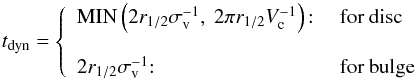$t_{dyn} = {\begin{matrix} MIN (2 r_{1 / 2} σ_{v}^{-1}, 2 π r_{1 / 2} {V_{c}^{-1}}^{)} : & fordisc \\ 2 r_{1 / 2} σ_{v}^{-1} : & forbulge \end{matrix}$ $\begin{equation} t_{\rm dyn} = \left\{ \begin{array}{ll} {\rm MIN}\left(2r_{1/2}\sigma_{\rm v}^{-1},~2\pi r_{1/2} V_{\rm c}^{-1}\right){:} & \mbox{ for disc} \\ & \\ 2r_{1/2}\sigma_{\rm v}^{-1}{:} & \mbox{ for bulge} \end{array}\right. \label{t_dyn} \end{equation}$ (2)where V_c is the circular velocity measured at the half radius mass, and σ_v is the mean velocity dispersion. For completeness, we add that the star formation is computed only if the projected star forming gas surface density Σ_g is higher than a given threshold $\log_{10} (Σ_{g}^{\min}) = 1 [M_{⊙} p c^{2}]$ $\hbox{$\log_{10}(\Sigma_{\rm g}^{\rm min})~=~1~[\Msun\, \rm pc^2]$}$ .

2.5. Supernovae feedback

In a given stellar population, massive stars evolve quickly and end their life as supernovae. This violent death injects gas and energy into the interstellar medium. The gas is heated, and a fraction can be ejected from the galaxy plane and feed the surrounding host-halo phase. In addition, these ejecta are at the origin of the metal enrichment of structures. Supernova feedback is therefore a crucial ingredient. In the majority of SAM (e.g. Kauffmann et al. 1993; Cole et al. 1994, 2000; Silk 2003; Hatton et al. 2003; Somerville et al. 2008), and according to some observational studies (e.g. Martin 1999; Heckman et al. 2000; Veilleux et al. 2005), the SN-reheating or SN-ejecta rate is linked to the SFR. As proposed by Dekel & Silk (1986), we computed the ejected mass rate due to supernovae by using kinetic energy conservation. Another paradigm based on momentum conservation could be used, but it has been shown by Dutton & van den Bosch (2009) that, in the low-mass regime, the energy-driven feedback is more efficient and leads to better results.

The ejected mass rate Ṁ_ej,SN due to SN is linked to the SFR Ṁ_⋆ by using the individual supernova kinetic energy as: $Ṁ ej, SN V_{wind}^{2} = 2 ε_{ej} η_{sn} E_{sn} Ṁ ⋆$ $\begin{equation} \dot{M}_{\rm ej,SN}V_{\rm wind}^2 = 2\varepsilon_{\rm ej}\eta_{\rm sn}E_{\rm sn}\dot{M}_{\star} \label{sn_feedback} \end{equation}$ (3)where we use $η_{sn} = 9.3 \times 10^{-3} M_{⊙}^{-1}$ $\hbox{$\eta_{\rm sn}=9.3\times 10^{-3}~\Msun^{-1}$}$ and an efficiency ε_ej = 0.3¹. The value used for this parameter is similar to the one applied in standard SAMs (e.g. Somerville et al. 2008; Guo et al. 2011).

To break the degeneracy between the ejected mass and the velocity of the wind, we must add a constraint on the wind velocity. We rely on Bertone et al. (2005) in which the wind velocity is linked to the star formation rate (Martin 1999). It seems to be independent of the galaxy morphology (Heckman et al. 2000; Frye et al. 2002). We therefore use Eq. (9) in Bertone et al. (2005) to model the wind velocity.

On average, wind velocities obtained with this prescription are higher than in other studies (e.g. Somerville et al. 2008; Dutton & van den Bosch 2009). Indeed it is common to use galaxy escape velocity to describe the wind, which is, for the ejection process, the minimum required value. Therefore, the ejected mass is at its maximum (see Dutton & van den Bosch 2009, their discussion in Sect. 7.3). Consequently, our loading factor (Ṁ_ej,SN/Ṁ_⋆) is smaller than in other models, and therefore our mean ejected mass is also lower. The difference between our reference model and standard supernova feedback is discussed in Sect. 3.2.

2.6. The active galaxy nucleus

A supermassive black hole (SMBH) can evolve in the centre of the bulge. We form the seed of the SMBH by converting a fraction of the bulge mass (gas and stars) to the SMBH mass, when the bulge mass becomes higher than a mass threshold M_bulge ≥ 10³M_bhM_⊙. This formation process is only turned on during a merger event. The SMBH formed at this time has a mass equal to M_bh = 10³ M_⊙. This mass is created by instantaneously converting a fraction of the gas and stars in their respective ratio. After its formation, the SMBH evolves in the centre of the bulge by accretion and clumps migration. The accretion process is mainly driven by the (Bondi 1952) accretion prescription, and we add an episodic accretion linked to clumps migration to this classical mechanism. This accretion is obviously limited by the maximum value of the Eddington accretion rate. As for supernovae, AGNs produce winds and contribute to the hot-atmosphere heating. We convert a given fraction of the power produced by mass accretion into kinetic and thermal power (f_Kin = 10^-3, e.g. Proga et al. 2000; Stoll et al. 2009; Ostriker et al. 2010). To compute the AGN ejected mass rate, we use the same kinetic conservation criterium as applied to supernovae: $Ṁ {}_{jet}V_{jet}^{2} \propto Ṁ {}_{agn}c^{2}$ $\hbox{$\dot{M}_{\rm jet}V_{\rm jet}^2 \propto \dot{M}_{\rm agn}c^2$}$ . Then we compute the momentum transfer between the AGN jet and the gas to estimate the mass that leaves the galaxy owing to AGN/gas coupling. We assume that all the mass is ejected with a velocity equal to the galaxy escape velocity ( $Ṁ_{ej, AGN} \propto Ṁ_{jet} \frac{V_{jet}}{V_{esc}}$ $\hbox{$\dot{M}_{\rm ej,AGN}\propto\dot{M}_{\rm jet}\frac{V_{\rm jet}}{V_{\rm esc}}$}$ ). As explained in Sect. 2.7, the thermal power of the AGN is used for the monitoring of the hot phase temperature.

Table 1

List of SAMs compared in this paper.

2.7. Hot-halo phase

As mentioned previously, galaxies hosted by massive dark matter haloes present a hot stable atmosphere generated by the hot cosmological accretion and maintained by galaxy ejecta. We use a new self consistent model for the hot halo phase evolution. We follow the hot halo phase mean temperature ( $T$ $\hbox{$\mean{T}$}$ ) by applying a conservation criterion on the energy produced by hot accretion and/or feedback winds coming from SN/AGN. For SN and AGN, a fixed fraction (f_Therm = 5%) of the non-kinetic energy is converted into wind-thermal energy.

In parallel to the mean temperature monitoring, we compute the evaporated mass² and mass loss due to galactic winds. All these calculations are done in a dominant dark-matter gravitational potential and assume the hydrostatic equilibrium (HEC; Suto et al. 1998; Makino et al. 1998; Komatsu & Seljak 2001; Capelo et al. 2012). This new model gives a mean temperature ( $T$ $\hbox{$\mean{T}$}$ ) close to the standard virial temperature prescription for structure in the intermediate dark matter halo mass range (10¹⁰−10¹² M_⊙). Low-mass structures have higher temperatures (≤2T_vir). This result is linked to the gas ionization fraction that is assumed to be the same for all structures. Massive structures that host an active galaxy nucleus also have higher mean temperatures, but never higher than three times the temperature derived from the standard virial assumption.

2.8. Cooling processes

Cooling is computed using the classical model initially proposed by White & Frenk (1991). The condensed mass enclosed in the cooling radius r_cool is estimated assuming:

an HEC gas profile ρ_g(r) (Suto et al. 1998; Makino et al. 1998; Komatsu & Seljak 2001; Capelo et al. 2012),
a mean constant temperature $T$ $\hbox{$\overline{T}$}$ ,
a temperature and metal dependent cooling function Λ(T,Z_g) (Sutherland & Dopita 1993).

The cooling radius r_cool is the unique solution for t(r_cool) = t_cool, where t_cool is the effective cooling time computed as the life time of the hot gas phase, and t(r) is the cooling time function of White & Frenk (1991) $t (r) = 0.64 \frac{m_{p} k_{b} T}{ρ_{g} (r) Λ [T, Z_{g}]} \cdot$ $\begin{equation} t(r) = 0.64\dfrac{m_{\rm p} k_{\rm b} \overline{T}}{\rho_{\rm g}(r)\Lambda[\overline{T},Z_{\rm g}]}\cdot \label{cooling_time_function} \end{equation}$ (4)

2.9. Mergers and bulge growth

At a given time step t_n, if two or more haloes have the same descendant at t^{n + 1}, these haloes and their host galaxies have merged during this time lapse. We assume that the merger occurs at t_merge = 0.5 × (t^{n + 1} + t_n)³. Between t_n and t_merge, the progenitors evolve in their host dark-matter halo and between t_merge and t^{n + 1} the remnant galaxy evolves in the descendent dark-matter halo. Even if more than two progenitors are identified, mergers are computed using dark-matter (and associated galaxy) pairs starting from the lower sub-halo mass to the higher main halo mass. The post-merger galaxy morphology depends on the mass (galaxy + dark-matter halo) ratio of the two progenitors. We define $η_{merger} = \frac{MIN (M_{1 / 2, 1}; M_{1 / 2, 2})}{MAX (M_{1 / 2, 1}; M_{1 / 2, 2})}$ $\begin{equation} \eta_{\rm merger} = \dfrac{{\rm MIN}(M_{1/2,1}{;}~M_{1/2,2})}{{\rm MAX}(M_{1/2,1}{;}~M_{1/2,2})} \label{mu_merger} \end{equation}$ (5)where M_1/2,i = M_gal,i(r<r_1/2) + 2M_dm,i(r<r_1/2) is, for system i, the sum of the galaxy and the dark matter halo mass enclosed in the galaxy half-mass radius (r_1/2).

For η_merge< 0.25, we consider that it is a minor merger. In this case, the disc and the pre-existing bulge component are kept, and gas and star contents are just added. The remnant disc size is set to the larger disc progenitor size. We apply the same rule to the bulge component. The velocities (dispersion and circular) of the bulge and the disc are recomputed with the properties of the remanent dark-matter halo. In the case of a major merger, η_merge> 0.25, progenitor discs are destroyed, and the remanent galaxy is only made of a bulge. The half mass radius of this spheroid is computed using the energy conservation and the virial theorem (as in Hatton et al. 2003). Like a pseudo-bulge component formed by giant clumps migration (Sect. 2.3), bulges are described by a Hernquist (1990) model. After a major merger event, all new accreted material generates a new disc component. The mass is only transferred to the bulge by disc instabilities (Sect. 2.3).

Mergers are violent events. On a short time scale, the galaxy properties are strongly modified, and secular evolution laws (efficiencies) are no longer valid. To take the modifications induced by a merger into account, we use a boost factor, MAX[ 1,ε_boost(Δt) ], that increases the efficiencies of star formation in each component of the galaxy (disc and bulge), and of SMBH accretion. The boost factor is defined as: $ε_{boost} (τ) = 100 η_{merger} η_{gas} \exp (- \frac{τ}{τ_{merger}})$ $\begin{equation} \varepsilon_{\rm boost}(\tau) = 100\eta_{\rm merger}\eta_{\rm gas}\exp\left(-\dfrac{\tau}{\tau_{\rm merger}}\right) \label{boost_factor} \end{equation}$ (6)where η_gas is the gas fraction in the post-merger structure, τ is the time elapsed since the last merger event, τ_merger = 0.05 Gyr is a characteristic merger-time scale and η_merger is given in Eq. (5). The formulation is used to simulate a time-dependent gas compression (decreasing with time) and takes the gas content of the two progenitors into account. The more gas they contain, the more the gas compression is high.

2.10. The adaptive time-step scheme

In a galaxy, various processes act at the same time on various time scales. For example, it is not efficient to compute the evolution of the cold filamentary phase, which evolves on a typical dark-matter dynamical time (10⁶ yr), with a time step following the ejection rate of the galaxy (10⁴ yr). Using the same time step for all components generates numerical errors on the slowly evolving component and degrades the precision. Each component of the baryonic halo or of the galaxy (disc and/or bulge) must evolve with a time step that is as close as possible to its dynamical time. Accordingly, we have developed an adaptive time-step scheme. Each halo or galaxy component has a separated evolution scheme, and interacts with others only if the mass transfers significantly affect its evolution. We consider that the mass reservoir is modified if the variation is over 10%.

Table 2

List of the main models parameters. The values given here are identical or very similar to those commonly used in the literature.

3. Star formation in the low-mass structures in standard models

We focus in this section on the main problem of star formation activity in low-mass structures. We explore various prescriptions for the photoionization or SN-feedback processes and compare the results with some fundamental galaxy properties: stellar mass function (SMF), M_h versus M_⋆ relation (SHMR), the sSFR versus M_⋆ relation, and SFR distribution (or IR-LF).

Table 1 gives the description of the models, from m₀ without feedback processes (in red) to m₄, where we put a large fraction of the gas into a no-star-forming gas component (see Sect. 4.2). In the low-mass range analysed here, AGN-feedback does not play an important role, and therefore it is not further discussed.

3.1. Impact of photoionization

Gas heating generated by the first generation of stars and quasars limits the baryonic gas accretion in the smaller structures (Kauffmann et al. 1993). The effective baryonic fraction $f_{b}^{ph - ion}$ $\hbox{$f_{\rm b}^{\rm ph-ion}$}$ (Eq. (7)) depends on both the redshift and the dark matter halo mass. The most commonly used formulation is the one proposed by Gnedin (2000) and Kravtsov et al. (2004): $f_{b}^{ph - ion} (M_{h},z) = ⟨ f_{b} ⟩ {[1 + (2^{α / 3} - 1) {(\frac{M_{h}}{M_{c} (z)})}^{- α}]}^{- 3 / α} \cdot$ $\begin{equation} f_{\rm b}^{\rm ph-ion}(M_{\rm h},z) = \left<f_{\rm b}\right>\left[1 + (2^{\alpha/3}-1)\left(\dfrac{M_{\rm h}}{M_{\rm c}(z)}\right)^{-\alpha}\right]^{-3/\alpha}\cdot \label{ph-ion} \end{equation}$ (7)In this definition, ⟨f_b⟩ is the universal baryonic fraction, M_h the dark matter halo mass, and M_c(z) the filtering mass corresponding to the mass where the halo lost half of its baryons. Finally, α is a free parameter that mainly controls the slope of the transition.

For α = 1, $f_{b}^{ph - ion} / ⟨ f_{b} ⟩$ $\hbox{$f_{\rm b}^{\rm ph-ion}/\left<f_{\rm b}\right>$}$ : 0 → 1 for M_h: 10⁹ → 10¹² M_⊙,
For α = 2, $f_{b}^{ph - ion} / ⟨ f_{b} ⟩$ $\hbox{$f_{\rm b}^{\rm ph-ion}/\left<f_{\rm b}\right>$}$ : 0 → 1 for M_h: 10⁹ → 10¹⁰ M_⊙.

The redshift evolution of the filtering mass M_c and the value of α are the crucial parameters governing the impact of photoionization on small structures.

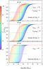Fig. 1

Normalized baryonic fraction $f_{b}^{ph - ion} / f_{b}$ $\hbox{$f_{\rm b}^{\rm ph-ion} /f_{\rm b}$}$ as a function of the dark matter halo mass. The colour code shows the redshift evolution (from z = 10 in red, to z = 0 in purple). We compare two different prescriptions for the evolution of the baryonic fraction after the redshift of reionization. The two upper panels are made using the Gnedin (2000) prescription with two different reionization redshifts (zreion =10 and 9). The bottom panel shows the Okamoto et al. (2008) prescription with zreion =9. The grey vertical line indicates our dark-matter mass resolution limits (20 dm-particles). In the Gnedin (2000) model (central panel) the strong effects induced by photoionization ( $f_{b}^{ph - ion} < 0.5 ⟨ f_{b} ⟩$ $\hbox{$f_{\rm b}^{\rm ph-ion} < 0.5\left<f_{\rm b}\right>$}$ ) appear at z ≃ 7−8 and become stronger with decreasing redshift. In the Okamoto et al. (2008) prescription, the impact of photoionization comes much later (z< 1) and cannot affect the galaxy formation processes at high z.

These parameters have been constrained using hydrodynamic simulations that include UV photoionization performed by, for example, Gnedin (2000), Kravtsov et al. (2004), Hoeft et al. (2006), or Okamoto et al. (2008). The analysis of these different simulations gives different results, and therefore various parameter values and filtering mass behaviours. While in Gnedin (2000) the slope index is set to (α = 1), Okamoto et al. (2008) find a higher value (α = 2). We recall in Appendix B the mathematical expressions for the two filtering masses given in these papers and used here.

In Fig. 1, we show the evolution of $f_{b}^{ph - ion}$ $\hbox{$f_{\rm b}^{\rm ph-ion}$}$ /⟨f_b⟩ for the two prescriptions. The two top panels are dedicated to the Gnedin (2000) model. Their filtering mass definition is the one most commonly used in the literature (Somerville 2002; Somerville et al. 2008, 2012; Croton et al. 2006; Guo et al. 2011). In the upper panel, we apply z_reion = 10, as in Somerville et al. (2012). In the central panel we apply z_reion = 9 to compare with Okamoto et al. (2008). The grey horizontal line marks a decrease of 50% comparing to the universal baryonic fraction. We consider that the photoionization effect is important when $f_{b}^{ph - ion} < 0.5 ⟨ f_{b} ⟩$ $\hbox{$f_{\rm b}^{\rm ph-ion} < 0.5 \left<f_{\rm b}\right>$}$ . The colour code indicates the redshift evolution.

At our dark matter halo mass resolution, in the first case (Gnedin 2000, z_reion = 10), photoionization starts to play a role at z ≃ 8. At low z, the small structures are strongly affected by the photoionization process. This trend is still true when the reionization redshift is decreased (central panel, z_reion = 9). The effect of photoionization is much less important in the Okamoto et al. (2008) prescription. Indeed, the significant decrease in $f_{b}^{ph - ion}$ $\hbox{$f_{\rm b}^{\rm ph-ion}$}$ /⟨f_b⟩ only appears at the mass resolution for redshift z< 1. In this case, the gas heating due to the UV background cannot affect, at high redshift, the baryonic assembly of small structures. This difference in behaviour comes from the different redshift evolutions of the filtering mass M_c(z). In the two cases, the authors use hydrodynamic simulations to constrain this evolution. As explained by Okamoto et al. (2008), even if the two studies use different assumptions (e.g. link between gas density and gas temperature), it seems that the difference between the two prescriptions is most likely due to insufficient resolution of the Gnedin (2000) simulation.

We applyed the two photoionization prescriptions in models m₁ and m₂. The first one, m₁, uses the Okamoto et al. (2008) description. It is our reference model. For comparison, we use Gnedin (2000) prescription in m₂. As we can see in Figs. 3 and 4, the two models mainly have an impact at low redshift. The figures show that the Gnedin (2000) prescription reduces the stellar mass formed in the small dark matter mass regime more than does the Okamoto et al. (2008) prescription. This is consistent with the baryonic fraction behaviour described above. Gas accretion is more reduced in the Gnedin (2000) model. At low halo mass (M_halo< 5 × 10¹⁰ M_⊙) and at low redshift (z< 2), the mean stellar mass built through the Gnedin (2000) photoionization model (m₂) may be ten times lower than the one built with the Okamoto et al. (2008) model (m₁).

Currently, the majority of SAMs use the Gnedin (2000) photoionization parameterization. The parameter set (α, M_c(z)) used in this case leads to an accretion rate on the galaxies that is reduced compared to what is obtained using Okamoto et al. (2008). This result fully agrees with Guo et al. (2011). However, regardless of the case, it is evident from Fig. 3 that photoionization is not enough to reduce the low-mass end of the stellar mass function as required by the observations.

3.2. Impact of SN feedback

While the photoionization process reduces the gas feeding of the galaxy, supernova feedback expels the gas already present in the galaxy. Despite their different actions, both processes tend to reduce the amount of gas available to form stars.

We compare two SN-feedback models:

our model based on kinetic, thermal energy conservation, hot gas phase heating, and evaporation;
the Somerville et al. (2008) model based on their Eqs. (12) and (13) (reheated rate and escape fraction). In this case, the hot gas-phase temperature is not monitored as it is in our model, but is set to the dark matter virial temperature.

As listed in Table 1, m₂ and m₃ used the same photoionization prescription (Gnedin 2000). They differ only in their SN-feedback model. A simple comparison between the stellar mass functions (Fig. 3) given by m₂ and model m₃ in which we have implemented the Somerville et al. (2008) prescription indicates that the SN-feedback mechanism is more efficient in their model. This difference is even more visible on the SHMR (Fig. 4) which indicates that the stellar mass produced in low-mass haloes (M_h< 10¹¹ M_⊙) is, on average, higher in our model by a factor close to 3. This difference decreases when z decreases and M_h increases.

As explained previously (Sect. 2.5), the higher mean wind velocity computed in our model following Bertone et al. (2005) leads to a lower ejected mass for a given kinetic energy. A more detailed comparison of the two models proves that the reheating rate computed with the Somerville et al. (2008) SN-feedback model (m₃) is, on average, for a given dark matter halo mass, twice more than with our ejected-rate (m₂). We see the same trend if we compare the two models at a fixed SFR.

The ejected-hot gas is transferred to the hot-halo phase. Its possible definitive ejection from the hot atmosphere is computed by assuming the dark-matter potential well, taking the velocity of the wind and the escape velocity of the dark matter structure into account. The gas mass that is definitively ejected is higher in m₂ than in m₃, on average, in the intermediate range of masses. This is linked to the wind velocity that is fixed to a value of about ≃100−150 km s^-1 in m₂ (see Eq. (13) in Somerville et al. 2008) and more than ~150 km s^-1, on average, in m₃⁴. This difference is at the origin of the break in the slope of the stellar-mass function between m₂ and m₃.

The large difference, at high mass, between m₂ and m₃ is due to the AGN feedback. For consistency reasons with our hot gas phase heating modelling (which associates both SN and AGN), we cannot apply the AGN-feedback processes in this Somerville et al. (2008) model comparison, while, in model m₂, our AGN feedback is turned on, and therefore reduces the stellar mass.

Despite the different parameterizations and energy injection scales for supernovae, currently the classical semi-analytical models do not seem to be able to explain the high-redshift behaviour of the mass function in the low-mass range (see also Fig. 23 in Guo et al. 2011; and Fig. 11 in Ilbert et al. 2013). Even if some SAMs, such as Somerville et al. (2008), Guo et al. (2011), or Henriques et al. (2013), use a dedicated parametrization to reproduce the galaxy properties at z = 0, it seems that, at high redshift, the low-mass range problem of the stellar-mass function is not only linked to a SN-feedback efficiency calibration. Indeed, Guo et al. (2011; their Figs. 8 and 23) show that the number of low-mass star-forming galaxies are still larger than observed. A new ad-hoc parametrization of the Guo et al. (2011) model is proposed by Henriques et al. (2013). Using a very high efficiency for the SN feedback coupled to a very low efficiency for the re-accretion of the gas (see Sect. 4.3 for a complete discussion), they obtain a better result in the low-mass regime.

A strong increase in the SN-wind efficiency in low-mass structures also leads to very high mass-loading factors (Ṁ_ej/Ṁ_⋆> 10, Henriques et al. 2013, their Fig. 3). Such factors are much greater that those derived from spectroscopic observations (e.g. Sturm et al. 2011; Rubin et al. 2011; Bouché et al. 2012) even if the measurement of this parameter is difficult and is currently performed on massive systems. In these conditions, stellar outflows alone cannot limit the star formation sufficiently. In this context, the measurement of the mass-loading factor becomes a key point.

4. An ad hoc recipe for reconciling models and observations

At high redshift (z> 1), as shown in Fig. 3, the amplitude of the faint end of the stellar mass function is dramatically over-estimated by the models (m₁, m₂ and m₃). This result is consistent with the overestimate of stellar mass in low-mass dark matter haloes: small structures form too many stars. In general, this problem is addressed by a strong SN feedback and/or photoionization. As shown previously, photoionization and SN-feedback cannot be sufficient to reduce significantly the star formation in low-mass objects. Strong feedback models give some good integrated results (at z ≃ 0) (Guo et al. 2011; De Lucia & Blaizot 2007) but fail at higher redshift (see Ilbert et al. 2013, their Fig. 11).

In this section we propose a strong modification of implementing of the star-formation mechanism in our semi-analytical model to try to reconcile models and observations.

4.1. Can all the cold gas form stars?

In a standard semi-analytical model, the SFR is adjusted to follow the observed empirical Kennicutt (1998) law. The rate is computed following Eq. (1) and is applied to the entire cold gas reservoir. In this context, the efficiency parameter ε_⋆ determines the fraction of star-forming gas. This fraction is obviously constant. The Kennicutt (1998) law reflects, with global variables, an overall view of the star formation process. Even if large reservoirs of gas are observed in galaxies, at least up to z ≃ 1.5 (e.g. Daddi et al. 2010), these observations do not give any information about the real fraction of the gas that is available to form stars.

The Kennicutt law and the homogeneous description of the cold gas cannot describe the complex structure of the ISM. Observations indicate that only a very small amount of the gas mass is used at a given time to form stars in galaxies (including ours); the star formation occurs only in highly-concentrated regions and not in the entire disc. Recent Herschel observations show that stars form in dense cold cores with a typical size of 0.1 pc, embedded in the interstellar filamentary structure (André et al. 2010; Heiderman et al. 2010; Lada et al. 2012). These prestellar cores are formed only when the gas surface density is higher than Σ_thr ≃ 160 M_⊙ yr^-1. Observations show that only a small amount of the total gas mass (≃15%) is above this column density threshold and only a small fraction (≃15%) of this dense gas is in the form of prestellar cores (André 2013; André et al. 2014). Therefore, a large amount of the gas is not available to form stars. This no-star-forming component corresponds to the gas that is occupying the low levels of matter structuration, where the gas surface density is low.

4.2. The no-star-forming disc component

When accreted on the galaxy disc, the surface density of fresh gas (considered as homogeneously distributed) is low. Progressively the gas, controlled by the turbulence and gravity energy balance, is structured more and more (Kritsuk & Norman 2011). The energy injected by the accretion process must be dissipated before star-formation process can start. Since the dissipation scale is much smaller than the energy injection scale, we assume that the energy cascade introduces a delay between the accretion time and the star formation time.

To model this process, we introduce a model m₄ with a new gas component in galaxy discs: the no-star-forming gas. The delay between the accretion time of fresh gas and the time when this gas is converted into stars is modelled by a transfer rate between the no-star-forming gas and the star-forming gas reservoir (g^⋆) that follows $Ṁ g^{⋆}, in = Ṁ g, out = ε_{⋆} \begin{matrix} \min \end{matrix} [1, {(\frac{M_{h}}{10^{12} M_{⊙}})}^{3}] \frac{M_{g}}{t_{dyn}}$ $\begin{equation} \dot{M}_{\sfg,\rm in} = \dot{M}_{\nosfg,\rm out} = \varepsilon_{\star}\min\left[1,\left(\dfrac{M_{\rm h}}{10^{12}~\Msun}\right)^3\right]\dfrac{M_{\nosfg}}{t_{\rm dyn}} \label{no-sfg2sfg} \end{equation}$ (8)where M_g is the mass of no-star-forming gas, t_dyn the disc dynamical time, and ε_⋆ an efficiency parameter, identical to the star formation efficiency (Eq. (1)). Obviously this formulation is totally ad hoc and does not provide any physical information on the link between the characteristic time of the turbulent cascade and the mass of the halo. The halo mass dependence in Eq. (8) is introduced to reproduce the shape of the stellar to halo mass relation, as observed in for example Leauthaud et al. 2012; Moster et al. 2010; Behroozi et al. 2010; Béthermin et al. 2012.This formulation has no other purpose. It does not describe the structuration of the density. However, the dependence in $M_{h}^{3}$ $\hbox{$M_{\rm h}^3$}$ indicates that the star formation regulation process must be extremely strong in the smallest structures. In the context of the bimodal accretion, the accretion is dominated by the cold mode below M_h = 10¹² M_⊙. This cold accretion is feeding the no-star-forming gas reservoir, which thus regulates the star formation in such structures.

In the context of this new prescription we decided to apply the merger boost factor (Eq. (6)) to the no-star-forming transfer process (Eq. (8)) and to the star formation. Indeed we consider that mergers increase the mean gas concentration instantaneously, and thus accelerate the structuration of the density.

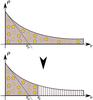Fig. 2

Radial density profile of the gas in the disc. While in a classical model (upper panel) all the gas is available to form stars and is distributed in the whole disc, the star-forming gas is artificially concentrated in the centre of the disc and the no-star-forming is distributed in the outer region with our ad hoc model (lower panel). The star-forming gas is enclosed in the radius r_s.

If the no-star-forming gas was homogeneously added to the disc structure, the decrease in the star-forming gas fraction would be equivalent to a simple decrease in the star formation efficiency ε_⋆. This is not satisfactory, and to maintain the star formation efficiency even with a large amount of no-star-forming gas, we thus had to adopt an artificial gas concentration, as illustrated in Fig. 2. Using this gas redistribution, we derive a new dynamical time, and thus SFR, from the circular velocity computed at the characteristic radius r_s. With this model, we can produce high SFR, even if a large amount of gas is considered as no-star-forming, without modifying the star formation recipes.

Fig. 3

Stellar mass function and its evolution with redshift. The redshift is increasing clockwise. The colour code is the same for all figures, and is detailed in the model list (Table 1). We compare our results with Ilbert et al. (2010, 2013; squares), Yang et al. (2009; circles), Baldry et al. (2008; triangles in the first panel), and Caputi et al. (2011; triangles) observations. Horizontal arrows show the link between the density and the number of haloes in our simulation volume. The grey dashed lines plotted in the high-mass range indicate the limit where uncertainties due to the cosmic variance are equal to the differences between models.

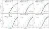Fig. 4

Stellar-to-dark-matter halo mass relation (SHMR) for various redshifts. The models (coloured lines) are compared with recent analysis based on halo occupation or abundance matching (black line: Moster et al. 2010; grey line: Béthermin et al. 2012; black open circles: Behroozi et al. 2010). While standard models have a regular evolution of the stellar mass with M_h, the ad hoc recipe included in m4 produces: i) a very slow increase of the stellar mass for haloes with M_h< 10¹¹ M_⊙; ii) a very strong increase of the stellar mass at intermediate halo mass (10¹¹<M_h< 10¹² M_⊙). This shape is not captured well by our points with error bars. The large error bar associated with the M_h = 10¹¹ M_⊙ point results from the very large scatter produced by the strong increase of the stellar mass in this halo mass range. iii) A slow increase in the stellar mass for M_h> 10¹² M_⊙.

4.3. Comparison with the Munich model

The current baseline of the Munich model is mainly described in Guo et al. (2011). Some important modifications are presented in Henriques et al. (2013). This paper focusses on the reincorporation of the ejected gas. The model is based on an ejecta reservoir that receives the gas ejected from the galaxy. The main hypothesis is that this gas is not available for cooling and it has to be reincorporated into the hot gas reservoir to cool. This ejecta reservoir, linked to the halo, is fed by the very efficient SN-feedback processes. As presented in Henriques et al. (2013) the key point of this model is the reincorporation timescale. In the current model, it is inversely proportional to the halo mass and is independent of redshift (from 1.8 × 10¹⁰ yr for haloes with M_h = 10¹⁰ M_⊙ to 1.8 × 10⁸ yr for haloes with M_h = 10¹² M_⊙). In this context, the gas expelled from low-mass structures is stored for a long time in the ejecta reservoir, so this model strongly limits the star formation process. In this scenario the no-star-forming gas is stored outside of the galaxy. This model gives good predictions in the low-mass range of the stellar mass function, but, without a prompt reincorporation of this gas in the cooling loop, the amount of star-forming gas, and therefore the star formation activity, are limited in the disc of low and intermediate-mass objects.

Regardless the mechanism behind it, it seems that the storage of the gas in a no-star-forming reservoir (e.g. reservoir of low-density gas in the disc, or reservoir without any cooling outside the galaxy) is the best way to modulate the star-formation efficiency such that semi-analytical models can reproduce the observations.

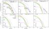Fig. 5

Gas mass functions predicted by our SAMs. The colour code is explained in Table 1. For comparison, we add the extremal gas mass function deduced from the dark-matter mass function and the universal baryonic fraction ⟨f_b⟩ (grey dashed-line). In the case of m₄, we plot the total (star-forming + no-star-forming) and the star-forming gas mass function. We compare our results with the molecular gas mass function computed by Berta et al. (2013; lower limits, circles) and with the local HI mass function computed by Zwaan et al. (2005; triangles). The black solid line shows the HI mass function predicted by Lagos et al. (2011), using Bower et al. (2006) SAM. The horizontal arrows show the link between the density and the number of haloes in our simulation volume.

5. Stellar and gas-mass assembly

We have presented different processes that act on galaxy formation and, more precisely, on the star formation activity. We tested two photoionization models and two supernovae feedback models. In addition to these four models, we have proposed another model in which we have strongly limited the star formation efficiency in low-mass haloes. In this section we discuss the comparison of this model with the main galaxy properties, and compare the predictions of this model in detail with the other four.

5.1. Stellar-mass function and SHMR

We show in Fig. 3 the stellar-mass functions predicted by our models. Model outputs are compared with observational data from Ilbert et al. (2010, 2013), Baldry et al. (2008), and Yang et al. (2009), Caputi et al. (2011).

As discussed before, models m₁, m₂, and m₃ fail to reproduce the low-mass end of the stellar mass function. The disagreement is both on the amplitude (one order of magnitude higher at low mass) and on the shape of the mass function. Figure 4 shows the stellar mass as a function of the dark-matter halo mass. We compare all models with relations extracted from the literature (Behroozi et al. 2010; Béthermin et al. 2012; Moster et al. 2010). This figure indicates that the excess of galaxies with low stellar masses is due to an over-production of stars in the low-mass dark matter haloes. To reduce this tension, we applied a strong modification of the star formation process in m₄. The gas is kept in the disc but, a large amount of this gas cannot form stars. With this ad hoc model, in the low mass range, the levels of the stellar mass functions are in good agreement with observations for a wide range of stellar masses. This indicates that only a strong modification (a decrease in our case) of the mass of gas instantaneously available to form stars allows the star formation activity in low mass structures to be modulated and SAM to be reconciled with the observations.

Concerning the high-mass end of the stellar-mass function, all models under-predict the number of massive galaxies. For z = 4 and z = 3, the comparison with Ilbert et al. (2010) and Ilbert et al. (2013) observational mass functions indicate that the massive galaxies in our models are two time less massive than the observed distribution. This is also observed in other recent SAMs (see e.g. Henriques et al. 2013, their Figs. 4−6, and Guo et al. 2011, their Fig. 23). The only way to reconcile models and observation in this high-mass regime is to consider a model without any regulation mechanism (model m₀). In contrast, for the low-redshift range (z = 0−2), our models give a small excess for massive galaxies. This disagreement could be linked to an AGN-feedback that is not efficient enough. The volume in the simulated box [(100 /h)³ ≃ 150³Mpc³] does not allow us to have more than ten haloes with mass higher than M_h = 10¹³ M_⊙, and therefore there is a small statistical sample associated to this range of mass. As we can see in Fig. 3 at z = 0.3 and for mass larger than 10¹¹ M_⊙, the stellar mass function is quite noisy. For information, we indicate, in each panel, the stellar mass above which uncertainties due to cosmic variance become larger than the differences between the models (see Appendix A for more details).

5.2. Gas-mass function

In m₄, we have chosen to modify the standard star formation paradigm, through the introduction of a delay between gas accretion and star formation. The step during which the no-star-forming gas is converted into star-forming gas strongly reduces the star formation activity, and therefore the stellar mass build-up. Obviously the total amount of gas in galaxies (no-star-forming and star-forming) will be strongly modified with respect to standard models. In this section, we compare the gas mass function predicted by all models with the available observational constraints.

In Fig. 5, we show the predicted gas-mass functions, together with the local HI mass function computed by Zwaan et al. (2005) and the molecular gas mass function coming from Berta et al. (2013). In their study, Berta et al. (2013) focus on the molecular gas contained in normal star-forming galaxies (within ± 0.5 dex in SFR from the main sequence). Quiescent galaxies are therefore not taken into account. In these conditions, and as explained by Berta et al. (2013), their data points should be considered as lower limits. The gas-mass functions extracted from our models are computed using all galaxies contained in our simulated volume, and taking the total gas mass in galaxy discs into account (both star-forming and no-star-forming).

The gas-mass functions predicted by our reference model m₁ and its variation (m₂) are very close. Indeed, the two models use the same prescription for gas ejection (sn + agn). At low mass and at all redshifts, the gas mass predicted by m₃ (using Somerville et al. 2008 sn feedback prescription) is also very close to m₁ and m₂. At high mass, the difference is due to SMBH. Indeed, in m₃ the SMBH activity is not taken into account. Consequently, the cooling rate associated with high-mass haloes is not limited, and the amount of gas increases.

In the case of the new model m₄, we plot in Fig. 5 the total and the star-forming gas-mass function. As expected, the amount of total gas in m₄ is larger than in the reference model m₁ or its variations (m₂ and m₃). The decrease in the star formation activity in m₄ leads to an large storage of the gas. In the first two panels (z ≃ 0 and z ≃ 1), the difference between the total and the star-forming gas mass functions is larger than at higher redshift; the fraction of no-star-forming gas increases with time. This evolution is linked to the transfer rate between the no-star-forming gas and the star-forming gas reservoirs (Eq. (8)). Indeed, for a given mass of no-star-forming gas, the rate increases with the dark-matter halo mass, but only up to M_h = 10¹² M_⊙. Above this threshold the rate is constant for a given mass of no-star-forming gas. Thus, for haloes more massive than M_h = 10¹² M_⊙, the fraction of no-star-forming is increasing.

Table 3

Gas-mass fractions at z = 0 of (a) HI gas w.r.t total gas in galaxy (gas); (b) star-forming gas (SFG) w.r.t. total gas in galaxy; (c) no-star-forming HI gas; (d) (HI−SFG) w.r.t. HI; (e) no star-forming & no HI gas w.r.t. no star-forming gas; (f) no-star-forming gas w.r.t baryon in the halo.

We also show in Fig. 5 the HI-mass fonction derived by Lagos et al. (2011) using the SAM of Bower et al. (2006). At first order, it is comparable to the mass-function evolution from our reference model m₁, which is reassuring and expected. It is interesting to note that their predictions for the low-mass range (M< 10⁹ M_⊙) are systematically higher than those predicted by our models at z> 0. This effect could be linked to some resolution effects. At z = 0, the reference model m₁ under-predicts the mass function at high mass, while the Lagos et al. (2011) model shows better agreement with the measured HI mass function. This difference can be due to a stronger SMBH feedback in our reference model. Under this hypothesis, in m₁, with less SMBH feedback, the accretion rate, hence the SFR, would be higher. This would increase the assembled stellar mass and thus the level of stellar mass function that is already too high in the high-mass range.

At z ≃ 0, the amount of total gas predicted by m₄ is larger than the measurement of the HI gas and the lower values of the molecular gas. Independently of each other, the HI and the molecular gas represent only a fraction of the total gas mass contained in a galaxy. However, we can note that for the high-mass range, the star-forming gas mass function predicted by m₄ is in good agreement with the HI mass function measured by Zwaan et al. (2005). Even if the total gas mass predicted by m₄ seems high, without any measurement of this total mass, it is difficult to conclude. The total gas mass function appears today as one of the key observables that will allow us to determine the optimal efficiency of gas ejection process and star formation.

We can integrate at z = 0 the HI-mass function measured by Zwaan et al. (2005) and the gas-mass function predicted by model m₄ in the mass range [ 10⁸,10¹² ] M_⊙ to compare the gas mass fractions in the different components (Table 3). If we gather the observed and the predicted values, these ratios indicate that:

only ≃2.5% of the total gas mass contained in a galaxy can be used directly to form a new generation of stars;
≃70% of the HI mass should be no-star-forming;
more than 90% of the no-star-forming gas is not detected in HI. This fraction is potentially greater than observed, even if its nature still has to be examined in the context of the “missing baryon problem”. It could be low-metallicity molecular gas or very hot (X-ray) diluted gas. For instance, some years ago Pfenniger et al. (1994) and Pfenniger & Combes (1994) proposed that there is a large amount of cold dark gas (essentially in molecular form, H2 in a fractal structure) evolving in the outer parts of galaxy discs. Following Pfenniger & Combes (1994), this gas could be no-star-forming and in equilibrium between coalescence, fragmentation, and disruption along a hierarchy of turbulent clumps. In these conditions, the dissipation time of this gas may exceed several Gyr, and only a tiny fraction may be turned into stars. This kind of hidden baryon could be a candidate for a physical explanation of the ad hoc model. As already explained, the total gas mass function appears as a key observable in the context of the new molecular gas surveys.

Comparing models and observations at higher redshift, we see from Fig. 5 that standard models strongly under-predict the amount of observed (molecular) gas, at least for z ≤ 2 in high-mass galaxies. At high masses (dark-matter halo + galaxy), the gas-ejection process is very limited. Thus, the lack of gas mass cannot be explained by an excessive instantaneous ejection in high-mass objects, but by a time-integrated ejection process that is too efficient.

At z ~ 2 the amount of molecular gas measured by Berta et al. (2013) is much greater than predicted by all models. Even if the observed gas quantity seems very large, the lack of gas in the models may explain the under-prediction of massive galaxies at these epochs (see Fig. 3).

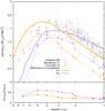Fig. 6

Redshift evolution of the star formation rate density. Model predictions (coloured lines) are compared with observational data (grey points) coming from Hopkins & Beacom (2006), Bouwens et al. (2011), and Cucciati et al. (2012). Solid lines present the star formation rates derived from the models. They are computed as the sum of the star formation rate of all galaxies and divided by the box volume ((100 /h)³ ≃ 150³ Mpc³). Dashed lines show the merger-driven star formation activity. The bottom panel gives the redshift evolution of the ratio ρ_sfr,burst/ρ_sfr,tot. We can see that the fraction of star formation activity linked to merger events is larger in m₄ than in the reference model m₁.

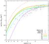Fig. 7

Redshift evolution of the stellar mass density from the models (coloured lines). Model predictions are compared with observational data (grey points) coming from Wilkins et al. (2008), Stark et al. (2009), and Labbé et al. (2010).

5.3. Star formation rate history

Figures 6 and 7 show the evolution with redshift of the cosmic SFR density (CSFRD) and the stellar mass density, respectively. Models are compared to a set of observational data: Hopkins & Beacom (2006), Bouwens et al. (2011), and Cucciati et al. (2012) for the SFR density, and Wilkins et al. (2008), Stark et al. (2009), and Labbé et al. (2010) for the stellar mass density. For the sake of clarity, only m₁ and m₄ are shown in Fig. 6. Models m₂ and m₃ lead to similar evolutions to model m₁.

Model m₁, with (SN/AGN)-feedback, presents a peak of CSFRD between z = 3 and z = 6 that is marginally compatible with observations. This early peak in star formation is at the origin of the over-production of stellar mass (Fig. 7) in the structures formed at this epoch (with M_halo ≤ 10¹¹ M_⊙). A strong SFR leads to a strong SN feedback, and consequently to a large amount of mass that definitively leaves the dark matter halo potential (≃60%). The gas density in the hot atmosphere becomes too low to produce efficient cooling, and the accretion rates for the galaxies decrease. For example, with our model m₁ at z = 2, the mean cooling rate on a 10^11.5 M_⊙ dark matter halo is 2.15 M_⊙ yr^-1. The cooling rate falls at 1.40 M_⊙ yr^-1 at z = 0.3, which is a decrease of 35%. This lack of fresh gas is at the origin of the strong decrease in the SFR found for m₁ at low redshifts (z< 3). Even if the boost factor (Eq. (6)) is applied to the post-merger galaxies, m₁ cannot correct for this lack of star formation. In the Munich model this decrease is compensated by the reincorporation of the gas previously expelled from the galaxy on a nadapted timescale, which allows increasing the gas mass available to cool.

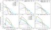Fig. 8

Star formation rate distribution for m₁, m₃, and m₄. Solid and dot-dashed coloured lines give the total and the merger-induced (Eq. (6)) star formation rate distribution, respectively. The merger-induced distributions are built with galaxies that i) have merged during the last time-step and ii) have $SFR > SFR + σ_{SFR}$ $\hbox{${\it SFR}>~\mean{{\it SFR}}+\sigma_{\rm SFR}$}$ , where $SFR$ $\hbox{$\mean{{\it SFR}}$}$ and σ_SFR are, respectively, the mean and standard deviation of star formation rate distribution of steady-state galaxies with stellar mass and dark matter halo mass value close (in the same half dex) to the merger-driven starburst galaxy taken into account. Models are compared with a set of observational data coming from Rodighiero et al. (2010; circles), Magnelli et al. (2011; squares) and Reddy et al. (2008; triangles) at low redshift (z ≤ 3), and from Smit et al. (2012; diamonds) at high redshift (z = 4−6). For information we add the free-fall rate (black dash-dot line) and cooling rate (black dot line) distribution function for model m₄.

The redshift evolutions of the CSFRD and stellar mass density predicted by m₄ are in better agreement with observations. Indeed, the strong reduction of the gas fraction available to form stars allows both reducing the star formation activity at high z and maintaining a larger amount of gas than in model m₁ at low z.

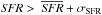
Figure 6 shows, the solid lines the total CSFRD. In the same plot we added a second measurement for information, where we have only taken the merger-driven star-forming galaxies. This kind of galaxy is defined as a post merger structure with a SFR boost (Eq. (6)) leading to SFR values greater than $SFR + σ_{SFR}$ $\hbox{$\mean{{\it SFR}}+\sigma_{\rm SFR}$}$ ⁵. In the steady-state galaxies, the SFR is closely linked to the fresh accretion of gas and is not due to recent merger events. We see from the figure that at high redshift (z ~ 3), in m₁, the stellar mass growth is dominated by the star formation in steady-state objects. As explained previously, in m₄ the merger driven star formation process is more efficient than in m₁. Indeed, even if we apply the merger-boosting factor (Eq. (6)) to the star formation of post-merger galaxies in m₁, they do not have enough gas to produce large starbursts.

Figure 7 gives a good summary of the situation. We see that for standard models (m₁, m₂ and m₃), the stellar mass is formed too early in the evolution histories of galaxies. Currently, standard SAMs (e.g. Somerville et al. 2008; Guo et al. 2011) are reproducing the local CSFRD and stellar-mass density quite well. But these good results at z = 0 must not obscure the fact that the history of the stellar mass assembly is not described well. Indeed, as shown in Fig. 7, the stellar mass densities predicted at z> 3 are systematically larger than the observations. The results obtained at z = 0 are only due to an excessive decrease in the mean SFR after the strong over-production of stars at high redshift. Indeed, as shown in Fig. 6, for z< 2 the CSFRD is systematically lower than observed. This decrease is also visible in the slope of the stellar mass density. If the gas is over-consumed at high z, it seems to be missing at low z. Only the ad hoc model that maintains a large amount of gas in discs allows reproducing at the same time i) the stellar mass density at all redshifts and ii) the trend in the CSFRD.

5.3.1. The star formation rate distribution

Figure 8 shows the SFR distribution function. We compare models m₁, m₃, and m₄ with a set of observational data. To obtain the SFR distribution we applied the standard conversions from infrared luminosity or ultraviolet magnitude measurements to SFR (Kennicutt 1998 conversions, with a Chabrier IMF, SFR [ M_⊙ yr^-1 ] = 3.1 × 10^-10L_{IR(8−1000 μm)} [ L_⊙ ]). In Fig. 8, we are also showing the total and merger-driven SFR. In all cases, the high SFR values are mainly linked to merger events, even if the boost factor generates a wide range of SFR.

As discussed previously, the lack of gas in galaxies formed in m₁ produces a lower CSFRD than observed at low redshift. As a result, the SFR distribution predicted by m₁ at low redshift (0 <z< 1.8 in the figure) is always lower than the observations by a factor 0.3 dex on average. For m₄, the artificial gas concentration allows a large star formation activity to be maintained even if the fraction of star-forming gas is low. This delayed star formation model gives a good match to the observation for 0 <z< 3. But this good result must be put inot context. Indeed the strong decrease applied to the star-formation rate in m₄ leads to a very low level of star formation at high redshift (z ≃ 6), as can be seen in Fig. 8. Even if it seems that we need to strongly reduce the star formation activity if we want to reproduce galaxy properties at low redshift (z< 3), the comparison with the Bouwens et al. (2007) measurements indicates that model m₄ clearly under-predicts the star formation rate at these epochs. The observations show that, in some structures at high redshift (as for Lyman break galaxies), stars are formed with very high efficiency. Also, modelling the high-redshift Lyman-Alpha emitters, Garel et al. (2012) found that a very high star-formation efficiency is needed to reproduce the luminosity function. Our model m₄ cannot produce these kinds of galaxies.

To reconcile the predicted star formation rate distribution with the observed one, but still producing the same amount of stellar mass in these objects at these epoch⁶, we need to have the same quantity of star-forming gas, but to reduce the dynamical time of the star formation process. To do that we could associate the star-forming gas component to denser regions, with smaller characteristic sizes. This is expected to give star formation rates that would be comparable to those predicted by m₁. The SFR distribution in m₁ is in good agreement with Bouwens et al. (2007) at very high z, even if the stellar mass produced in these low-mass haloes is higher than observed. In this model, the rhythm of star formation is good, but the star formation acts on gas reservoirs that are too large. The star formation activity produced by m₃ (based on Somerville et al. 2008 SN-feedback), compared to the reference model m₁, under-predicts this high-redshift star-forming population. This is probably due to the strong photoionization and SN-feedback processes considered in this model.

Measurements of star formation rate, given by Reddy et al. (2008) and Bouwens et al. (2007), are computed using UV observations, corrected from dust extinction. This correction is based on the UV continuum/β-slope extinction law and is mainly an extrapolation of results from local galaxies (e.g. Burgarella et al. 2005). Even if this relation seems to be valid at redshift z ≃ 2 (e.g. Daddi et al. 2007; Reddy et al. 2012), it has a huge scatter, and extrapolations to large redshifts lead to large errors (especially at high SFR) that are difficult to estimate.

For completeness, we added the distribution function of the filamentary accretion rate to Fig. 8 and the cooling rate for m₄. As expected, the cold mode efficiency decreases when redshift decreases. At high SFR, it is interesting to note that no galaxy is accreting enough baryons to form stars in a steady-state mode; only the episodic merger events can produce these high values.

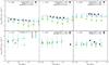Fig. 9

Specific star formation rate as a function of the stellar mass for a set of redshifts (the redshift is increasing clockwise). This quantity can be seen as the inverse of the stellar mass doubling time. The higher the value, the more intense the star formation activity. We compare the models (colour−coded) with observational data from Dunne et al. (2009), Karim et al. (2011), Gonzalez et al. (2012), Reddy et al. (2012), and Béthermin et al. (2012). For most observational data points, errors are smaller than the size of the symbol.

5.3.2. The specific star formation rate

Figure 9 shows the sSFR. We compare all models with a set of observations from Dunne et al. (2009); Karim et al. (2011); Gonzalez et al. (2012); Reddy et al. (2012) and with Béthermin et al. (2012) model predictions. First, for all models we note that the mean sSFR (over the whole mass range) increases with redshift. More specifically, we show in Fig. 10 the redshift evolution of the sSFR, extracted from model m₄, for two mass ranges. We see that more massive galaxies have lower sSFR at any redshift, implying that they form the bulk of their stars earlier than their low-mass counterparts.

At all redshift z ≤ 3 and for the whole mass range, models m₁ and m₂ are systematically lower (by a factor 10) than the observations. This result is due, on the one hand, to the low SFR as seen in Fig. 8, and on the other to the excess of stellar mass as seen in Fig. 4.

The model with stronger SN-feedback (m₃) gives better results in the intermediate redshift and mass ranges (0 <z< 3 ; 10¹⁰<M_⋆< 10¹¹ M_⊙) but stays lower than the observations in the lower mass regime for the same reasons as explained previously. The predictions at high mass suffer from the absence of AGN-feedback and do not have to be considered.

Model m₄ gives better agreement with the observations than the reference model m₁ or its variation m₂ does. In m₄, the mean star-formation efficiency is higher. This result does not contradict with the main objective of this ad-hoc model. The star formation activity is strongly reduced, and thus the produced stellar mass is also strongly reduced. This two trends lead to a higher level of the sSFR than in m₁ and m₂.

Figure 11 shows the sSFR distributions of galaxies predicted by model m₄ in a limited stellar mass range such that they can be directly compared with the Sargent et al. (2012) observational measurements. The population of quiescent galaxies has been removed in Sargent et al. (2012), we added two log-normal distributions to our histograms to allow for a better comparison:

a first one fit the MS population;
a second one fit the merger-driven population.

The excess of objects at low sSFR in the histograms, in comparison to the MS log-normal distribution, corresponds to the quiescent galaxy population.

We can see that the MS distribution predicted by m₄ is in excellent agreement with Sargent et al. (2012). However, the number of galaxies in the PMSB mode is over-predicted even if the average values of the distribution is in good agreement with what is observed (log ₁₀(sSFR/SFR_MS) ≃ 0.6). It is possible to reduce this tension by modifying our PMSB definition (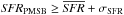 ${SFR}_{PMSB} \geq SFR + σ_{SFR}$ $\hbox{${\it SFR}_{\rm PMSB} \ge \overline{{\it SFR}}+\sigma_{\rm SFR}$}$ ). If we replace σ_SFR by 2σ_SFR in the previous definition, the number of objects on the PMSB population obviously decreases and becomes comparable to Sargent et al. (2012), but in this case, the centroid of the PMSB distribution is then shifted to a higher value (log ₁₀(sSFR/SFR_MS) ≃ 1). The properties of the PMSB population are also strongly dependent of the merger-boost factor used in the model (Eq. (6)). Some modifications, such as on the amplitude of the characteristic merger time scale (τ_merger), will be explored in a future work.

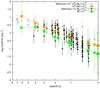Fig. 10

Redshift evolution of the specific star formation rate derived from m₄ (10⁸<M_⋆< 10¹⁰ M_⊙ in orange and 10¹⁰<M_⋆< 10¹² M_⊙ in green). The error bars correspond to the standard deviation. For comparison, we show the data points around M_⋆ = 10⁹ M_⊙ and M_⋆ = 10¹⁰ M_⊙, extracted from Behroozi et al. (2013b).

Fig. 11

Specific star formation rate distributions derived from model m₄, for galaxies with a stellar mass in the range: 10 < log ₁₀(M_⋆) < 10.33. The purple solid histogram shows the distribution of galaxies in the steady state mode (SFR ∝ accretion rate). Such a distribution contains main sequence (MS) and quiescent galaxies (sSFR/SFR_MS< 0.1 in our study). The purple dashed-line histogram shows the distribution of the sSFR for galaxies with post-merger star-formation activity (PMSB) (Eq. (6) and following ${SFR}_{PMSB} \geq SFR + σ_{SFR}$ $\hbox{${\it SFR}_{\rm PMSB} \ge \overline{{\it SFR}}+\sigma_{\rm SFR}$}$ ). At z = 2 we compare our results with Sargent et al. (2012) measurements in which the quiescent population have been removed (grey solid line). For a better comparison with these observational measurements, we add a log-normal distribution as a black solid line adjusted only on our MS galaxy population. We have removed all galaxies with sSFR/SFR_MS< 0.1. We see that model m₄ is in very good agreement with the MS distribution but over-predicts the number of galaxy in the post-merger starburst mode (0.4 dex).

5.4. Steady-state versus merger-driven star formation

To summarize, galaxies evolve in a quasi-steady state in m₁, m₂, and m₃, after the high level of star formation activity at 4 <z< 6, and consequently the high rates of mass ejection. The star-formation rate is directly proportional to the gas-accretion rate. At intermediate mass (M_h ≃ 10¹¹ M_⊙), there is not enough hot gas in equilibrium in the dark-matter potential well (owing to the strong feedback), and therefore the cooling is not efficient. Consequently, these intermediate-mass galaxies are deficient in fresh gas, and the star-formation rate becomes lower than observed at 1 <z< 3 (Figs. 8 and 6). In Guo et al. (2011) and Henriques et al. (2013), the lack of gas in the hot phase is compensated for by the reincorporation of the gas ejected previously that was stored in a passive reservoir.

In the delayed star formation model m₄, the amount of the star formation rate occurring in merger events and amplified by the boost factor is higher than in m₁ (see Fig. 8). Indeed, mergers generate a strong increase in the star formation activity because of the large amount of the accreted gas that is in the disc in the no-star-forming phase and to the merger-induced no-star-forming to star-forming gas conversion (Eqs. (8) and (6)). The rapid transformation of gas into stars allows reaching very high star-formation rates (see Fig. 8). At lower redshift, as in standard models, the larger amount of stellar mass is formed in the quasi-steady state mode. Even if, at these epochs, the contribution of merger events strongly decreases, the highest star formation rates are still found in post-merger structures.

6. Discussion and conclusion

We have presented four galaxy formation models and compared them. We showed that classical models m₁ (reference), m₂, and m₃ fail to reproduce the faint end of the stellar-mass function. They over-predict the stellar mass in the low-mass dark matter haloes (M_h< 10¹⁰ M_⊙). Even when a strong photoionization and SN-feedback are used (as in m₂ and m₃), the models form too many stars in the low-mass range. Moreover, recent observations indicate that the loading factors (Ṁ_ej/Ṁ_⋆) are much smaller that those predicted by such models. A strong SN-feedback generates a strong decrease in the amount of gas, which has to be compensated for at low z, for example, by reincorporating some gas (Henriques et al. 2013). Such a problem in the low-mass structures is invariably present, even in the most recent SAMs (Guo et al. 2011; Bower et al. 2012; Weinmann et al. 2012) and, as explained by Henriques et al. (2013), can thus be viewed as a generic problem.

On the basis of a comparison between the models for which the stellar-mass functions and the relationship between M_h and M_⋆ are reproduced quite well at z = 0 (e.g. Guo et al. 2011), it seems that the problem occurs at high redshift. But, if the relations at high z are not reproduced, then the history of the structures populating the relations at lower redshift is not consistent, even if the stellar-mass functions at these low redshifts seem agrees with observations.

If we consider that the Λ-CDM paradigm produces the correct number of low-mass dark matter haloes, then the star formation activity has to be strongly reduced in this range of masses to reproduce the observations. We applied this condition in an ad-hoc model (m₄). This model is based on a two-phase gaseous disc with, on the one hand the star-forming gas, and on the other, the no-star-forming gas. We showed that m₄ is in good agreement with a large set of observations, even if there is a tension with the z> 4 SFR computed from UV measurements (Bouwens et al. 2007).

A galaxy formation and evolution model that uses a strong modification of the star formation activity (quenched or limited) has already been studied by Bouché et al. (2010). In their model, the fresh gas accretion is halted for haloes with masses lower than M_h = 10¹¹ M_⊙. In our model, such small structures host a very large amount of no-star-forming gas. That this gas has been accreted but cannot form star leads to the same result as the non-accretion model proposed by Bouché et al. (2010). The results, produced by the toy model described in Bouché et al. (2010), are in good agreement with observations (sSFR, their Fig. 4, and the Tully-Fisher relation, their Fig. 5). This independent study reinforces the hypothesis of a strong decrease in the star formation efficiency in low-mass structures at high redshift.

In classical SAMs, the cold gas that can form star is modelled as a homogeneous component, generally following a decreasing radial exponential profile. In addition, these models consider that a given fraction of the gas is available to form stars at any moment. The SFR applied to this cold gas reservoir is computed following Kennicutt (1998) empirical law, without knowing the exact fraction of the gas that can actually be impacted by the process. The ad hoc model presented in this paper is based on a no-star-forming gas component that can be seen as the gaseous fraction that is not in optimal conditions forming stars, i.e., not above the critical density threshold.

Observations show that only a small fraction of the total gas mass (≃15%) is above the optimal column density threshold, and only a small fraction (≃15%) of this dense gas is in prestellar cores (André 2013; André et al. 2014). Indeed, before being in the form of a prestellar core, the gas in the ISM must follow a continuous structuration process, from the low density accreted gas to the highest density regions. This structuration cascade needs time and obviously, at a given time, all the gas in the disc cannot be available to form stars. The no-star-forming to star-forming conversion process may be linked to the global dynamic of the disc. Indeed in highly-disturbed discs (with a V/σ_v ∈ [ 1−10 ]), as observed at high z (e.g. Genzel et al. 2006, 2008; Stark et al. 2008; Cresci et al. 2009) and seen in hydrodynamic simulations (e.g. Kereš et al. 2005; Dekel et al. 2009a,b; Khochfar & Silk 2009), star formation occurs only in a few high-density regions (clumps).

In addition to these large scale disturbed dynamics at high z, the density structuration process can be limited by other mechanisms that are seen at low z. The turbulence heating can be one of them. Even if the main driver of this turbulence is not clearly understood (shocks, SN kinetic energy injection, tidal interactions, galaxy collisions), recent infrared spectroscopic observations at intermediate redshift (1 <z< 2) show that the molecular gas can be dynamically heated by turbulence (e.g. Guillard et al. 2009, 2012; Ogle et al. 2010; Appleton et al. 2013) and is thus not available for star formation. Hydrodynamic simulations by Bournaud et al. (2010) also show that the SN energy injection disrupts the dense regions on the smallest scales (ten to hundred parsecs) from the typical size of star-forming filaments in the ISM to a typical disc-scale height at z ≃ 2.

The main idea behind the no-star-forming gas reservoir is that, at any given time, only a fraction of the gas can form stars. Indeed even if Kennicutt’s law gives a relation between the gas content (mass), the geometry (galaxy size), and the star formation activity, it does not give any information about the gas fraction that is turned into stars. In a galaxy, a set of highly concentrated star-forming regions that affect a small amount of the total gas mass can be compatible with the Kennicutt’s law (sum of SFR in all regions). However, our ad-hoc model m₄ leads to a fraction of no-star-forming gas at z = 0 that is greater than given by observations. Our analysis can also be compared to previous works that introduced a significant fraction of gas that cannot form stars (e.g. Pfenniger et al. 1994; Pfenniger & Combes 1994). In this context, the study of the gas dynamics and states (with ALMA for instance) will be a key point in understanding the regulation of star formation in galaxies.

To model the two-phase disc, we assumed that the accreted gas is composed of a large fraction (99%) of no-star-forming gas, that is progressively converted in the star-forming phase. The conversion rate (Eq. (8)) has not been defined to explicitly and physically follow the structuration process but is calibrated to reproduce the SHMR (e.g. Leauthaud et al. 2012; Moster et al. 2010; Behroozi et al. 2010; Béthermin et al. 2012). This formulation has no other purpose than to highlight the order of magnitude of the regulation process that has to be introduced. To reproduce Kennicutt’s law on a galaxy scale, even when a large fraction of the gas can not form stars, we have artificially concentrated the star-forming gas in the centre of the disc where the density is the highest. This ad-hoc modification leads to very good results mainly for the stellar-mass functions and sSFR. On the other hand, the SFR distribution predicted by this model strongly disagrees with SFR measurements at z> 4. It shows the need for an explicit description of the density structuration process. The gas-mass function predicted by the ad-hoc model may indicate that galaxies have a gas content that is too large, even if the comparison with observations is difficult because the total gas mass function is not known. In the future measuring the gas mass function will be a key observable that will constrain the balance between the ejection process and gas regulation in galaxies.

In a forthcoming work, we plan to follow the structuration of the gas, using a semi-analytical approach from the largest scales (r>h, the disc-scale height), where the dynamics are governed by (quasi-)2D turbulence, to the smallest scales (r<h), where the star formation process occurs in 3D molecular clouds (Romeo et al. 2010; Bournaud et al. 2010). In current SAMs, the SFR is only linked to the gas component and to the overall galaxy dynamics (t_dyn). This approach is not able to correctly describe the regulation of the star formation. Galaxy discs are complex structures based on multi-fluid interactions on multi-scales (2D, 3D; Shi et al. 2011). The connexions between the stellar and gas components generate instabilities that participate in the ISM structuration (e.g. Jog & Solomon 1984; Hoffmann & Romeo 2012). Star formation and disc instabilities are thus strongly linked. A better description of these ISM structuration mechanisms is essential for a better understanding of the star formation regulation processes.

¹

The influence of the efficiency value has been tested in the range ε_ej ∈ [ 0.05,10 ]. Obviously a strong increase in the SN-efficiency increases the amount of ejected gas. The star formation activity is therefore reduced, but this effect affects only the amplitude and not the shape of the stellar mass function. Moreover, looking at the amplitude, its decrease is not enough to be in agreement with the observations.

²

The hot atmosphere is considered in hydrostatic equilibrium in the dark matter halo potential well. We use a Maxwell-Boltzmann function to describe the velocity distribution. At each time step, the mass corresponding to the hot gas that has higher velocities than the escape velocity of the halo is definitively removed.

³

However, even if we accurately follow the sub-haloes and if the merging time laps is reduced, the instantaneous merging of galaxies is always a strong assumption and could be explored in detail in a future work.

⁴

For a given kinetic energy the larger the wind velocity, the smaller the mass ejected mass.

⁵

$SFR$ $\hbox{$\mean{{\it SFR}}$}$ and σ_SFR are respectively the average and the standard deviation of SFR distribution of steady-state galaxies with stellar mass and dark matter halo mass value close (in the same half dex) to the merger-driven starburst galaxy that was considered.

⁶

Indeed, as shown in the stellar mass function, the build-up of the stellar mass agrees with the observed stellar mass function.

Acknowledgments

The authors thank Jean-loup Puget and Pierre Guillard for very useful comments and discussions. We also thank the referee for a very helpful report. We acknowledge financial support from the “Programme National de Cosmologie and Galaxies” (PNCG) of CNRS/INSU, France.

References

André, P. 2013 [arXiv:1309.7762] [Google Scholar]
André, P., Men’shchikov, A., Bontemps, S., et al. 2010, A&A, 518, L102 [NASA ADS] [CrossRef] [EDP Sciences] [Google Scholar]
André, P., Di Francesco, J., Ward-Thompson, D., et al. 2014, in Protostars and Planets VI, eds. H. Beuther, R. Klessen, C. Dullemond, & Th. Henning (University of Arizona Press), accepted [arXiv:1312.6232] [Google Scholar]
Appleton, P. N., Guillard, P., Boulanger, F., et al. 2013, ApJ, accepted [arXiv:1309.1525] [Google Scholar]
Babul, A., & Rees, M. J. 1992, MNRAS, 255, 346 [NASA ADS] [CrossRef] [Google Scholar]
Baldry, I. K., Glazebrook, K., & Driver, S. P. 2008, MNRAS, 388, 945 [NASA ADS] [Google Scholar]
Baugh, C. M. 2006, Rep. Prog. Phys., 69, 3101 [NASA ADS] [CrossRef] [Google Scholar]
Behroozi, P. S., Conroy, C., & Wechsler, R. H. 2010, ApJ, 717, 379 [NASA ADS] [CrossRef] [Google Scholar]
Behroozi, P. S., Wechsler, R. H., & Conroy, C. 2013a, ApJ, 762, L31 [NASA ADS] [CrossRef] [Google Scholar]
Behroozi, P. S., Wechsler, R. H., & Conroy, C. 2013b, ApJ, 770, 57 [NASA ADS] [CrossRef] [Google Scholar]
Bell, E. F., Zheng, X. Z., Papovich, C., et al. 2007, ApJ, 663, 834 [NASA ADS] [CrossRef] [Google Scholar]
Benson, A. J., Lacey, C. G., Baugh, C. M., Cole, S., & Frenk, C. S. 2002, MNRAS, 333, 156 [NASA ADS] [CrossRef] [Google Scholar]
Berta, S., Lutz, D., Nordon, R., et al. 2013, A&A, 555, L8 [NASA ADS] [CrossRef] [EDP Sciences] [Google Scholar]
Bertone, S., Stoehr, F., & White, S. D. M. 2005, MNRAS, 359, 1201 [NASA ADS] [CrossRef] [Google Scholar]
Béthermin, M., Doré, O., & Lagache, G. 2012, A&A, 537, L5 [NASA ADS] [CrossRef] [EDP Sciences] [Google Scholar]
Blumenthal, G. R., Faber, S. M., Primack, J. R., & Rees, M. J. 1984, Nature, 311, 517 [NASA ADS] [CrossRef] [Google Scholar]
Blumenthal, G. R., Faber, S. M., Flores, R., & Primack, J. R. 1986, ApJ, 301, 27 [NASA ADS] [CrossRef] [MathSciNet] [Google Scholar]
Bondi, H. 1952, MNRAS, 112, 195 [NASA ADS] [CrossRef] [MathSciNet] [Google Scholar]
Bouché, N., Dekel, A., Genzel, R., et al. 2010, ApJ, 718, 1001 [NASA ADS] [CrossRef] [Google Scholar]
Bouché, N., Hohensee, W., Vargas, R., et al. 2012, MNRAS, 426, 801 [NASA ADS] [CrossRef] [Google Scholar]
Bournaud, F., Elmegreen, B. G., & Elmegreen, D. M. 2007, ApJ, 670, 237 [Google Scholar]
Bournaud, F., Daddi, E., Elmegreen, B. G., et al. 2008, A&A, 486, 741 [NASA ADS] [CrossRef] [EDP Sciences] [Google Scholar]
Bournaud, F., Elmegreen, B. G., Teyssier, R., Block, D. L., & Puerari, I. 2010, MNRAS, 409, 1088 [NASA ADS] [CrossRef] [Google Scholar]
Bouwens, R. J., Illingworth, G. D., Franx, M., & Ford, H. 2007, ApJ, 670, 928 [NASA ADS] [CrossRef] [Google Scholar]
Bouwens, R. J., Illingworth, G. D., Oesch, P. A., et al. 2011, ApJ, 737, 90 [NASA ADS] [CrossRef] [Google Scholar]
Bower, R. G., Benson, A. J., Malbon, R., et al. 2006, MNRAS, 370, 645 [NASA ADS] [CrossRef] [Google Scholar]
Bower, R. G., Benson, A. J., & Crain, R. A. 2012, MNRAS, 422, 2816 [NASA ADS] [CrossRef] [Google Scholar]
Brinchmann, J., Charlot, S., White, S. D. M., et al. 2004, MNRAS, 351, 1151 [NASA ADS] [CrossRef] [Google Scholar]
Bullock, J. S., Kravtsov, A. V., & Weinberg, D. H. 2000, ApJ, 539, 517 [NASA ADS] [CrossRef] [Google Scholar]
Burgarella, D., Buat, V., & Iglesias-Páramo, J. 2005, MNRAS, 360, 1413 [NASA ADS] [CrossRef] [Google Scholar]
Capelo, P. R., Coppi, P. S., & Natarajan, P. 2012, MNRAS, 422, 686 [NASA ADS] [CrossRef] [Google Scholar]
Caputi, K. I., Cirasuolo, M., Dunlop, J. S., et al. 2011, MNRAS, 413, 162 [NASA ADS] [CrossRef] [Google Scholar]
Ceverino, D., Dekel, A., & Bournaud, F. 2010, MNRAS, 404, 2151 [NASA ADS] [Google Scholar]
Ceverino, D., Dekel, A., Mandelker, N., et al. 2012, MNRAS, 420, 3490 [NASA ADS] [CrossRef] [Google Scholar]
Chabrier, G. 2003, PASP, 115, 763 [NASA ADS] [CrossRef] [Google Scholar]
Chary, R., & Elbaz, D. 2001, ApJ, 556, 562 [NASA ADS] [CrossRef] [Google Scholar]
Cole, S. 1991, ApJ, 367, 45 [NASA ADS] [CrossRef] [Google Scholar]
Cole, S., Aragon-Salamanca, A., Frenk, C. S., Navarro, J. F., & Zepf, S. E. 1994, MNRAS, 271, 781 [NASA ADS] [CrossRef] [Google Scholar]
Cole, S., Lacey, C. G., Baugh, C. M., & Frenk, C. S. 2000, MNRAS, 319, 168 [NASA ADS] [CrossRef] [Google Scholar]
Conroy, C., & Wechsler, R. H. 2009, ApJ, 696, 620 [NASA ADS] [CrossRef] [Google Scholar]
Couchman, H. M. P., & Rees, M. J. 1986, MNRAS, 221, 53 [NASA ADS] [CrossRef] [Google Scholar]
Cousin, M., Lagache, G., Béthermin, M., & Guiderdoni, B. 2015, A&A, 575, A33 [NASA ADS] [CrossRef] [EDP Sciences] [Google Scholar]
Cowie, L. L., Hu, E. M., & Songaila, A. 1995, AJ, 110, 1576 [NASA ADS] [CrossRef] [Google Scholar]
Cresci, G., Hicks, E. K. S., Genzel, R., et al. 2009, ApJ, 697, 115 [NASA ADS] [CrossRef] [Google Scholar]
Croton, D. J., Springel, V., White, S. D. M., et al. 2006, MNRAS, 365, 11 [NASA ADS] [CrossRef] [Google Scholar]
Cucciati, O., Tresse, L., Ilbert, O., et al. 2012, A&A, 539, A31 [NASA ADS] [CrossRef] [EDP Sciences] [Google Scholar]
Daddi, E., Dickinson, M., Morrison, G., et al. 2007, ApJ, 670, 156 [NASA ADS] [CrossRef] [Google Scholar]
Daddi, E., Bournaud, F., Walter, F., et al. 2010, ApJ, 713, 686 [NASA ADS] [CrossRef] [Google Scholar]
De Lucia, G., & Blaizot, J. 2007, MNRAS, 375, 2 [NASA ADS] [CrossRef] [Google Scholar]
Dekel, A., & Silk, J. 1986, ApJ, 303, 39 [NASA ADS] [CrossRef] [Google Scholar]
Dekel, A., Birnboim, Y., Engel, G., et al. 2009a, Nature, 457, 451 [NASA ADS] [CrossRef] [PubMed] [Google Scholar]
Dekel, A., Sari, R., & Ceverino, D. 2009b, ApJ, 703, 785 [Google Scholar]
Doroshkevich, A. G., Zel’dovich, Y. B., & Novikov, I. D. 1967, Sov. Ast., 11, 233 [Google Scholar]
Dunne, L., Ivison, R. J., Maddox, S., et al. 2009, MNRAS, 394, 3 [NASA ADS] [CrossRef] [Google Scholar]
Dutton, A. A., & van den Bosch, F. C. 2009, MNRAS, 396, 141 [NASA ADS] [CrossRef] [Google Scholar]
Efstathiou, G. 1992, MNRAS, 256, 43P [Google Scholar]
Elbaz, D., Dickinson, M., Hwang, H. S., et al. 2011, A&A, 533, A119 [NASA ADS] [CrossRef] [EDP Sciences] [Google Scholar]
Elmegreen, B. G. 2009, in Galaxy Evolution: Emerging Insights and Future Challenges, eds. S. Jogee, I. Marinova, L. Hao, & G. A. Blanc, ASP Conf. Ser., 419, 23 [Google Scholar]
Elmegreen, B. G., & Elmegreen, D. M. 2005, ApJ, 627, 632 [NASA ADS] [CrossRef] [Google Scholar]
Faucher-Giguère, C.-A., Kereš, D., & Ma, C.-P. 2011, MNRAS, 417, 2982 [NASA ADS] [CrossRef] [Google Scholar]
Frye, B., Broadhurst, T., & Benítez, N. 2002, ApJ, 568, 558 [NASA ADS] [CrossRef] [Google Scholar]
Fu, L., Semboloni, E., Hoekstra, H., et al. 2008, A&A, 479, 9 [NASA ADS] [CrossRef] [EDP Sciences] [Google Scholar]
Garel, T., Blaizot, J., Guiderdoni, B., et al. 2012, MNRAS, 422, 310 [NASA ADS] [CrossRef] [Google Scholar]
Genzel, R., Tacconi, L. J., Eisenhauer, F., et al. 2006, Nature, 442, 786 [NASA ADS] [CrossRef] [PubMed] [Google Scholar]
Genzel, R., Burkert, A., Bouché, N., et al. 2008, ApJ, 687, 59 [NASA ADS] [CrossRef] [Google Scholar]
Gispert, R., Lagache, G., & Puget, J. L. 2000, A&A, 360, 1 [NASA ADS] [Google Scholar]
Gnedin, N. Y. 2000, ApJ, 542, 535 [NASA ADS] [CrossRef] [Google Scholar]
Gonzalez, V., Bouwens, R., llingworth, G., et al. 2012 [arXiv:1208.4362] [Google Scholar]
Granato, G. L., Lacey, C. G., Silva, L., et al. 2000, ApJ, 542, 710 [NASA ADS] [CrossRef] [Google Scholar]
Gruppioni, C., Pozzi, F., Andreani, P., et al. 2010, A&A, 518, L27 [NASA ADS] [CrossRef] [EDP Sciences] [Google Scholar]
Guiderdoni, B., Bouchet, F. R., Puget, J.-L., Lagache, G., & Hivon, E. 1997, Nature, 390, 257 [NASA ADS] [CrossRef] [Google Scholar]
Guillard, P., Boulanger, F., Pineau Des Forêts, G., & Appleton, P. N. 2009, A&A, 502, 515 [NASA ADS] [CrossRef] [EDP Sciences] [Google Scholar]
Guillard, P., Boulanger, F., Pineau des Forêts, G., et al. 2012, ApJ, 749, 158 [NASA ADS] [CrossRef] [Google Scholar]
Guo, Q., White, S., Boylan-Kolchin, M., et al. 2011, MNRAS, 413, 101 [NASA ADS] [CrossRef] [Google Scholar]
Hatton, S., Devriendt, J. E. G., Ninin, S., et al. 2003, MNRAS, 343, 75 [NASA ADS] [CrossRef] [Google Scholar]
Heckman, T. M., Lehnert, M. D., Strickland, D. K., & Armus, L. 2000, ApJS, 129, 493 [NASA ADS] [CrossRef] [MathSciNet] [Google Scholar]
Heiderman, A., Evans, II, N. J., Allen, L. E., Huard, T., & Heyer, M. 2010, ApJ, 723, 1019 [NASA ADS] [CrossRef] [Google Scholar]
Henriques, B. M. B., White, S. D. M., Thomas, P. A., et al. 2013, MNRAS, 431, 3373 [NASA ADS] [CrossRef] [Google Scholar]
Hernquist, L. 1990, ApJ, 356, 359 [NASA ADS] [CrossRef] [Google Scholar]
Hoeft, M., Yepes, G., Gottlöber, S., & Springel, V. 2006, MNRAS, 371, 401 [NASA ADS] [CrossRef] [Google Scholar]
Hoekstra, H., Yee, H. K. C., & Gladders, M. D. 2004, ApJ, 606, 67 [NASA ADS] [CrossRef] [Google Scholar]
Hoffmann, V., & Romeo, A. B. 2012, MNRAS, 425, 1511 [NASA ADS] [CrossRef] [Google Scholar]
Hopkins, A. M., & Beacom, J. F. 2006, ApJ, 651, 142 [NASA ADS] [CrossRef] [MathSciNet] [Google Scholar]
Ikeuchi, S. 1986, Ap&SS, 118, 509 [NASA ADS] [CrossRef] [Google Scholar]
Ilbert, O., Salvato, M., Le Floc’h, E., et al. 2010, ApJ, 709, 644 [NASA ADS] [CrossRef] [Google Scholar]
Ilbert, O., McCracken, H. J., Le Fevre, O., et al. 2013, A&A, 556, A55 [NASA ADS] [CrossRef] [EDP Sciences] [Google Scholar]
Jog, C. J., & Solomon, P. M. 1984, ApJ, 276, 114 [NASA ADS] [CrossRef] [Google Scholar]
Karim, A., Schinnerer, E., Martínez-Sansigre, A., et al. 2011, ApJ, 730, 61 [NASA ADS] [CrossRef] [Google Scholar]
Kauffmann, G., White, S. D. M., & Guiderdoni, B. 1993, MNRAS, 264, 201 [NASA ADS] [CrossRef] [Google Scholar]
Kennicutt, Jr., R. C. 1998, ApJ, 498, 541 [NASA ADS] [CrossRef] [Google Scholar]
Kereš, D., Katz, N., Weinberg, D. H., & Davé, R. 2005, MNRAS, 363, 2 [NASA ADS] [CrossRef] [Google Scholar]
Khochfar, S., & Silk, J. 2009, ApJ, 700, L21 [NASA ADS] [CrossRef] [Google Scholar]
Komatsu, E., & Seljak, U. 2001, MNRAS, 327, 1353 [NASA ADS] [CrossRef] [Google Scholar]
Kravtsov, A. V., Gnedin, O. Y., & Klypin, A. A. 2004, ApJ, 609, 482 [NASA ADS] [CrossRef] [Google Scholar]
Kritsuk, A. G., & Norman, M. L. 2011 [arXiv:1111.2827] [Google Scholar]
Labbé, I., González, V., Bouwens, R. J., et al. 2010, ApJ, 708, L26 [NASA ADS] [CrossRef] [Google Scholar]
Lada, C. J., Forbrich, J., Lombardi, M., & Alves, J. F. 2012, ApJ, 745, 190 [NASA ADS] [CrossRef] [Google Scholar]
Lagos, C. D. P., Baugh, C. M., Lacey, C. G., et al. 2011, MNRAS, 418, 1649 [NASA ADS] [CrossRef] [Google Scholar]
Le Floc’h, E., Papovich, C., Dole, H., et al. 2005, ApJ, 632, 169 [NASA ADS] [CrossRef] [Google Scholar]
Le Floc’h, E., Aussel, H., Ilbert, O., et al. 2009, ApJ, 703, 222 [NASA ADS] [CrossRef] [Google Scholar]
Leauthaud, A., Finoguenov, A., Kneib, J.-P., et al. 2010, ApJ, 709, 97 [NASA ADS] [CrossRef] [Google Scholar]
Leauthaud, A., Tinker, J., Bundy, K., et al. 2012, ApJ, 744, 159 [NASA ADS] [CrossRef] [Google Scholar]
Lilly, S. J., Le Fevre, O., Hammer, F., & Crampton, D. 1996, ApJ, 460, L1 [NASA ADS] [CrossRef] [Google Scholar]
Lu, Y., Kereš, D., Katz, N., et al. 2011, MNRAS, 416, 660 [NASA ADS] [CrossRef] [Google Scholar]
Madau, P., Ferguson, H. C., Dickinson, M. E., et al. 1996, MNRAS, 283, 1388 [NASA ADS] [CrossRef] [Google Scholar]
Magnelli, B., Elbaz, D., Chary, R. R., et al. 2011, A&A, 528, A35 [Google Scholar]
Makino, N., Sasaki, S., & Suto, Y. 1998, ApJ, 497, 555 [NASA ADS] [CrossRef] [Google Scholar]
Mandelbaum, R., Hirata, C. M., Broderick, T., Seljak, U., & Brinkmann, J. 2006a, MNRAS, 370, 1008 [NASA ADS] [CrossRef] [Google Scholar]
Mandelbaum, R., Seljak, U., Cool, R. J., et al. 2006b, MNRAS, 372, 758 [NASA ADS] [CrossRef] [Google Scholar]
Martin, C. L. 1999, ApJ, 513, 156 [NASA ADS] [CrossRef] [Google Scholar]
McKay, T. A., Sheldon, E. S., Racusin, J., et al. 2001 [arXiv:astro-ph/0108013] [Google Scholar]
Mo, H. J., Mao, S., & White, S. D. M. 1998, MNRAS, 295, 319 [Google Scholar]
Monaco, P., Fontanot, F., & Taffoni, G. 2007, MNRAS, 375, 1189 [NASA ADS] [CrossRef] [Google Scholar]
Moster, B. P., Somerville, R. S., Maulbetsch, C., et al. 2010, ApJ, 710, 903 [NASA ADS] [CrossRef] [Google Scholar]
Noeske, K. G., Weiner, B. J., Faber, S. M., et al. 2007, ApJ, 660, L43 [Google Scholar]
Ogle, P., Boulanger, F., Guillard, P., et al. 2010, ApJ, 724, 1193 [NASA ADS] [CrossRef] [Google Scholar]
Okamoto, T., Gao, L., & Theuns, T. 2008, MNRAS, 390, 920 [NASA ADS] [CrossRef] [Google Scholar]
Ostriker, J. P., Choi, E., Ciotti, L., Novak, G. S., & Proga, D. 2010, ApJ, 722, 642 [NASA ADS] [CrossRef] [Google Scholar]
Peacock, J. A., Cole, S., Norberg, P., et al. 2001, Nature, 410, 169 [NASA ADS] [CrossRef] [PubMed] [Google Scholar]
Peebles, P. J. E. 1969, ApJ, 155, 393 [NASA ADS] [CrossRef] [Google Scholar]
Pfenniger, D., & Combes, F. 1994, A&A, 285, 94 [NASA ADS] [Google Scholar]
Pfenniger, D., Combes, F., & Martinet, L. 1994, A&A, 285, 79 [NASA ADS] [Google Scholar]
Planck Collaboration XVI. 2014, A&A, 571, A16 [NASA ADS] [CrossRef] [EDP Sciences] [Google Scholar]
Proga, D., Stone, J. M., & Kallman, T. R. 2000, ApJ, 543, 686 [NASA ADS] [CrossRef] [Google Scholar]
Quinn, T., Katz, N., & Efstathiou, G. 1996, MNRAS, 278, L49 [NASA ADS] [CrossRef] [Google Scholar]
Reddy, N. A., Steidel, C. C., Pettini, M., et al. 2008, ApJS, 175, 48 [NASA ADS] [CrossRef] [Google Scholar]
Reddy, N. A., Pettini, M., Steidel, C. C., et al. 2012, ApJ, 754, 25 [NASA ADS] [CrossRef] [Google Scholar]
Rees, M. J. 1986, MNRAS, 218, 25P [Google Scholar]
Rodighiero, G., Vaccari, M., Franceschini, A., et al. 2010, A&A, 515, A8 [NASA ADS] [CrossRef] [EDP Sciences] [Google Scholar]
Romeo, A. B., Burkert, A., & Agertz, O. 2010, MNRAS, 407, 1223 [NASA ADS] [CrossRef] [Google Scholar]
Rubin, K. H. R., Prochaska, J. X., Ménard, B., et al. 2011, ApJ, 728, 55 [NASA ADS] [CrossRef] [Google Scholar]
Sargent, M. T., Béthermin, M., Daddi, E., & Elbaz, D. 2012, ApJ, 747, L31 [NASA ADS] [CrossRef] [Google Scholar]
Shapiro, P. R., Giroux, M. L., & Babul, A. 1994, ApJ, 427, 25 [NASA ADS] [CrossRef] [Google Scholar]
Shi, Y., Helou, G., Yan, L., et al. 2011, ApJ, 733, 87 [NASA ADS] [CrossRef] [Google Scholar]
Silk, J. 2003, MNRAS, 343, 249 [NASA ADS] [CrossRef] [MathSciNet] [Google Scholar]
Smit, R., Bouwens, R. J., Franx, M., et al. 2012, ApJ, 756, 14 [NASA ADS] [CrossRef] [Google Scholar]
Somerville, R. S. 2002, ApJ, 572, L23 [NASA ADS] [CrossRef] [Google Scholar]
Somerville, R. S., Hopkins, P. F., Cox, T. J., Robertson, B. E., & Hernquist, L. 2008, MNRAS, 391, 481 [NASA ADS] [CrossRef] [Google Scholar]
Somerville, R. S., Gilmore, R. C., Primack, J. R., & Domínguez, A. 2012, MNRAS, 423, 1992 [NASA ADS] [CrossRef] [Google Scholar]
Spergel, D. N., Verde, L., Peiris, H. V., et al. 2003, ApJS, 148, 175 [NASA ADS] [CrossRef] [Google Scholar]
Stark, D. P., Swinbank, A. M., Ellis, R. S., et al. 2008, Nature, 455, 775 [NASA ADS] [CrossRef] [PubMed] [Google Scholar]
Stark, D. P., Ellis, R. S., Bunker, A., et al. 2009, ApJ, 697, 1493 [NASA ADS] [CrossRef] [Google Scholar]
Stoll, R., Mathur, S., Krongold, Y., & Nicastro, F. 2009 [arXiv:0903.5310] [Google Scholar]
Sturm, E., González-Alfonso, E., Veilleux, S., et al. 2011, ApJ, 733, L16 [NASA ADS] [CrossRef] [Google Scholar]
Sutherland, R. S., & Dopita, M. A. 1993, ApJS, 88, 253 [NASA ADS] [CrossRef] [Google Scholar]
Suto, Y., Sasaki, S., & Makino, N. 1998, ApJ, 509, 544 [NASA ADS] [CrossRef] [Google Scholar]
Thoul, A. A., & Weinberg, D. H. 1996, ApJ, 465, 608 [NASA ADS] [CrossRef] [Google Scholar]
Toomre, A. 1963, ApJ, 138, 385 [NASA ADS] [CrossRef] [Google Scholar]
Toomre, A. 1964, ApJ, 139, 1217 [NASA ADS] [CrossRef] [Google Scholar]
Tweed, D., Devriendt, J., Blaizot, J., Colombi, S., & Slyz, A. 2009, A&A, 506, 647 [NASA ADS] [CrossRef] [EDP Sciences] [Google Scholar]
van de Voort, F., Schaye, J., Booth, C. M., Haas, M. R., & Dal la Vecchia, C. 2011, MNRAS, 414, 2458 [NASA ADS] [CrossRef] [Google Scholar]
van den Bergh, S. 1996, AJ, 112, 2634 [NASA ADS] [CrossRef] [Google Scholar]
Veilleux, S., Cecil, G., & Bland-Hawthorn, J. 2005, ARA&A, 43, 769 [Google Scholar]
Weinmann, S. M., Pasquali, A., Oppenheimer, B. D., et al. 2012, MNRAS, 426, 2797 [NASA ADS] [CrossRef] [Google Scholar]
White, S. D. M., & Frenk, C. S. 1991, ApJ, 379, 52 [NASA ADS] [CrossRef] [Google Scholar]
Wilkins, S. M., Trentham, N., & Hopkins, A. M. 2008, MNRAS, 385, 687 [NASA ADS] [CrossRef] [Google Scholar]
Yang, X., Mo, H. J., & van den Bosch, F. C. 2009, ApJ, 695, 900 [NASA ADS] [CrossRef] [Google Scholar]
Zwaan, M. A., Meyer, M. J., Staveley-Smith, L., & Webster, R. L. 2005, MNRAS, 359, L30 [NASA ADS] [CrossRef] [Google Scholar]

Appendix A: Cosmic variance

For the sake of clarity, errors bars due to cosmic variance in the stellar mass function are not plotted in Fig. 3. We have indicated a threshold above which uncertainties become larger than the variations observed for the different models. For illustration, we show in Fig. A.1 the stellar mass functions predicted by the models at z = 0.3, where we have added the error bars linked to the cosmic variance.

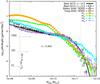Fig. A.1

Stellar mass function predicted by our different models at z = 0.3. The colour code is given in Table 1. We compare our results with Ilbert et al. (2010, 2013; squares), Yang et al. (2009; circles) and Baldry et al. (2008; triangles) observations. Horizontal arrows show the link between the density and the number of haloes in our simulation volume. We show in this figure the error bars related to cosmic variance.

Appendix B: The photoionization filtering masses

We used two different models of photoionization based on two definitions of the filtering mass. We recall here the expressions that we have used.

Appendix B.1: Prescription for m₁

For the Okamoto et al. (2008) model, we used an expression deduced from a fit of the filtering mass evolution given in their Fig. 15: $M_{c} (z) = 6 \times 10^{9} h_{0}^{-1} \exp (- 0.7 z^{)} M_{⊙} .$ $\appendix \setcounter{section}{2} \begin{equation} M_{\rm c}(z) = 6\times 10^{9}~h_0^{-1}\exp\left(-0.7z\right)~\Msun. \end{equation}$ (B.1)

Appendix B.2: Prescription for m₂

In Gnedin (2000) and Kravtsov et al. (2004), the filtering mass is defined as a function of the expansion factor (a): $M_{c} (a) = 2.5 \times 10^{11} h^{-1} Ω_{m}^{- 1 / 2} μ^{- 3 / 2} f (a) M_{⊙}$ $\appendix \setcounter{section}{2} \begin{equation} M_{\rm c}(a) = 2.5\times 10^{11}h^{-1}\Omega_{\rm m}^{-1/2}\mu^{-3/2}f(a)~\Msun \label{MB_dist} \end{equation}$ (B.2)where f(a) is the conditional function given in Eq. (B.3). As explained in Kravtsov et al. (2004), the best agreement with hydrodynamic simulations is obtained with α = 6. 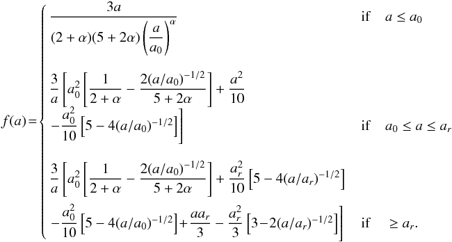$\begin{matrix} f (a) = \end{matrix}$ $\appendix \setcounter{section}{2} \begin{eqnarray} \label{condi_function} f(a)\! = \end{eqnarray}$ (B.3)

Appendix C: Data repository

Outputs from all models are available at the CDS. Data are distributed under *.fits format and are therefore compatible with the TOPCAT software (http://www.star.bris.ac.uk/~mbt/topcat/).

All Tables

Table 1

List of SAMs compared in this paper.

In the text

Table 2

List of the main models parameters. The values given here are identical or very similar to those commonly used in the literature.

In the text

Table 3

Gas-mass fractions at z = 0 of (a) HI gas w.r.t total gas in galaxy (gas); (b) star-forming gas (SFG) w.r.t. total gas in galaxy; (c) no-star-forming HI gas; (d) (HI−SFG) w.r.t. HI; (e) no star-forming & no HI gas w.r.t. no star-forming gas; (f) no-star-forming gas w.r.t baryon in the halo.

In the text

All Figures

Fig. 1

Normalized baryonic fraction $f_{b}^{ph - ion} / f_{b}$ $\hbox{$f_{\rm b}^{\rm ph-ion} /f_{\rm b}$}$ as a function of the dark matter halo mass. The colour code shows the redshift evolution (from z = 10 in red, to z = 0 in purple). We compare two different prescriptions for the evolution of the baryonic fraction after the redshift of reionization. The two upper panels are made using the Gnedin (2000) prescription with two different reionization redshifts (zreion =10 and 9). The bottom panel shows the Okamoto et al. (2008) prescription with zreion =9. The grey vertical line indicates our dark-matter mass resolution limits (20 dm-particles). In the Gnedin (2000) model (central panel) the strong effects induced by photoionization ( $f_{b}^{ph - ion} < 0.5 ⟨ f_{b} ⟩$ $\hbox{$f_{\rm b}^{\rm ph-ion} < 0.5\left<f_{\rm b}\right>$}$ ) appear at z ≃ 7−8 and become stronger with decreasing redshift. In the Okamoto et al. (2008) prescription, the impact of photoionization comes much later (z< 1) and cannot affect the galaxy formation processes at high z.

In the text

	Fig. 2 Radial density profile of the gas in the disc. While in a classical model (upper panel) all the gas is available to form stars and is distributed in the whole disc, the star-forming gas is artificially concentrated in the centre of the disc and the no-star-forming is distributed in the outer region with our ad hoc model (lower panel). The star-forming gas is enclosed in the radius r_s.
In the text

Fig. 3

Stellar mass function and its evolution with redshift. The redshift is increasing clockwise. The colour code is the same for all figures, and is detailed in the model list (Table 1). We compare our results with Ilbert et al. (2010, 2013; squares), Yang et al. (2009; circles), Baldry et al. (2008; triangles in the first panel), and Caputi et al. (2011; triangles) observations. Horizontal arrows show the link between the density and the number of haloes in our simulation volume. The grey dashed lines plotted in the high-mass range indicate the limit where uncertainties due to the cosmic variance are equal to the differences between models.

In the text

Fig. 4

Stellar-to-dark-matter halo mass relation (SHMR) for various redshifts. The models (coloured lines) are compared with recent analysis based on halo occupation or abundance matching (black line: Moster et al. 2010; grey line: Béthermin et al. 2012; black open circles: Behroozi et al. 2010). While standard models have a regular evolution of the stellar mass with M_h, the ad hoc recipe included in m4 produces: i) a very slow increase of the stellar mass for haloes with M_h< 10¹¹ M_⊙; ii) a very strong increase of the stellar mass at intermediate halo mass (10¹¹<M_h< 10¹² M_⊙). This shape is not captured well by our points with error bars. The large error bar associated with the M_h = 10¹¹ M_⊙ point results from the very large scatter produced by the strong increase of the stellar mass in this halo mass range. iii) A slow increase in the stellar mass for M_h> 10¹² M_⊙.

In the text

Fig. 5

Gas mass functions predicted by our SAMs. The colour code is explained in Table 1. For comparison, we add the extremal gas mass function deduced from the dark-matter mass function and the universal baryonic fraction ⟨f_b⟩ (grey dashed-line). In the case of m₄, we plot the total (star-forming + no-star-forming) and the star-forming gas mass function. We compare our results with the molecular gas mass function computed by Berta et al. (2013; lower limits, circles) and with the local HI mass function computed by Zwaan et al. (2005; triangles). The black solid line shows the HI mass function predicted by Lagos et al. (2011), using Bower et al. (2006) SAM. The horizontal arrows show the link between the density and the number of haloes in our simulation volume.

In the text

Fig. 6

Redshift evolution of the star formation rate density. Model predictions (coloured lines) are compared with observational data (grey points) coming from Hopkins & Beacom (2006), Bouwens et al. (2011), and Cucciati et al. (2012). Solid lines present the star formation rates derived from the models. They are computed as the sum of the star formation rate of all galaxies and divided by the box volume ((100 /h)³ ≃ 150³ Mpc³). Dashed lines show the merger-driven star formation activity. The bottom panel gives the redshift evolution of the ratio ρ_sfr,burst/ρ_sfr,tot. We can see that the fraction of star formation activity linked to merger events is larger in m₄ than in the reference model m₁.

In the text

	Fig. 7 Redshift evolution of the stellar mass density from the models (coloured lines). Model predictions are compared with observational data (grey points) coming from Wilkins et al. (2008), Stark et al. (2009), and Labbé et al. (2010).
In the text

Fig. 8

Star formation rate distribution for m₁, m₃, and m₄. Solid and dot-dashed coloured lines give the total and the merger-induced (Eq. (6)) star formation rate distribution, respectively. The merger-induced distributions are built with galaxies that i) have merged during the last time-step and ii) have $SFR > SFR + σ_{SFR}$ $\hbox{${\it SFR}>~\mean{{\it SFR}}+\sigma_{\rm SFR}$}$ , where $SFR$ $\hbox{$\mean{{\it SFR}}$}$ and σ_SFR are, respectively, the mean and standard deviation of star formation rate distribution of steady-state galaxies with stellar mass and dark matter halo mass value close (in the same half dex) to the merger-driven starburst galaxy taken into account. Models are compared with a set of observational data coming from Rodighiero et al. (2010; circles), Magnelli et al. (2011; squares) and Reddy et al. (2008; triangles) at low redshift (z ≤ 3), and from Smit et al. (2012; diamonds) at high redshift (z = 4−6). For information we add the free-fall rate (black dash-dot line) and cooling rate (black dot line) distribution function for model m₄.

In the text

Fig. 9

Specific star formation rate as a function of the stellar mass for a set of redshifts (the redshift is increasing clockwise). This quantity can be seen as the inverse of the stellar mass doubling time. The higher the value, the more intense the star formation activity. We compare the models (colour−coded) with observational data from Dunne et al. (2009), Karim et al. (2011), Gonzalez et al. (2012), Reddy et al. (2012), and Béthermin et al. (2012). For most observational data points, errors are smaller than the size of the symbol.

In the text

	Fig. 10 Redshift evolution of the specific star formation rate derived from m₄ (10⁸<M_⋆< 10¹⁰ M_⊙ in orange and 10¹⁰<M_⋆< 10¹² M_⊙ in green). The error bars correspond to the standard deviation. For comparison, we show the data points around M_⋆ = 10⁹ M_⊙ and M_⋆ = 10¹⁰ M_⊙, extracted from Behroozi et al. (2013b).
In the text

Fig. 11

Specific star formation rate distributions derived from model m₄, for galaxies with a stellar mass in the range: 10 < log ₁₀(M_⋆) < 10.33. The purple solid histogram shows the distribution of galaxies in the steady state mode (SFR ∝ accretion rate). Such a distribution contains main sequence (MS) and quiescent galaxies (sSFR/SFR_MS< 0.1 in our study). The purple dashed-line histogram shows the distribution of the sSFR for galaxies with post-merger star-formation activity (PMSB) (Eq. (6) and following ${SFR}_{PMSB} \geq SFR + σ_{SFR}$ $\hbox{${\it SFR}_{\rm PMSB} \ge \overline{{\it SFR}}+\sigma_{\rm SFR}$}$ ). At z = 2 we compare our results with Sargent et al. (2012) measurements in which the quiescent population have been removed (grey solid line). For a better comparison with these observational measurements, we add a log-normal distribution as a black solid line adjusted only on our MS galaxy population. We have removed all galaxies with sSFR/SFR_MS< 0.1. We see that model m₄ is in very good agreement with the MS distribution but over-predicts the number of galaxy in the post-merger starburst mode (0.4 dex).

In the text

Fig. A.1

Stellar mass function predicted by our different models at z = 0.3. The colour code is given in Table 1. We compare our results with Ilbert et al. (2010, 2013; squares), Yang et al. (2009; circles) and Baldry et al. (2008; triangles) observations. Horizontal arrows show the link between the density and the number of haloes in our simulation volume. We show in this figure the error bars related to cosmic variance.

In the text

Current usage metrics show cumulative count of Article Views (full-text article views including HTML views, PDF and ePub downloads, according to the available data) and Abstracts Views on Vision4Press platform.

Data correspond to usage on the plateform after 2015. The current usage metrics is available 48-96 hours after online publication and is updated daily on week days.

Initial download of the metrics may take a while.

[1] André, P. 2013 [arXiv:1309.7762] [Google Scholar]

[2] André, P., Men’shchikov, A., Bontemps, S., et al. 2010, A&A, 518, L102 [NASA ADS] [CrossRef] [EDP Sciences] [Google Scholar]

[3] André, P., Di Francesco, J., Ward-Thompson, D., et al. 2014, in Protostars and Planets VI, eds. H. Beuther, R. Klessen, C. Dullemond, & Th. Henning (University of Arizona Press), accepted [arXiv:1312.6232] [Google Scholar]

[4] Appleton, P. N., Guillard, P., Boulanger, F., et al. 2013, ApJ, accepted [arXiv:1309.1525] [Google Scholar]

[5] Babul, A., & Rees, M. J. 1992, MNRAS, 255, 346 [NASA ADS] [CrossRef] [Google Scholar]

[6] Baldry, I. K., Glazebrook, K., & Driver, S. P. 2008, MNRAS, 388, 945 [NASA ADS] [Google Scholar]

[7] Baugh, C. M. 2006, Rep. Prog. Phys., 69, 3101 [NASA ADS] [CrossRef] [Google Scholar]

[8] Behroozi, P. S., Conroy, C., & Wechsler, R. H. 2010, ApJ, 717, 379 [NASA ADS] [CrossRef] [Google Scholar]

[9] Behroozi, P. S., Wechsler, R. H., & Conroy, C. 2013a, ApJ, 762, L31 [NASA ADS] [CrossRef] [Google Scholar]

[10] Behroozi, P. S., Wechsler, R. H., & Conroy, C. 2013b, ApJ, 770, 57 [NASA ADS] [CrossRef] [Google Scholar]

[11] Bell, E. F., Zheng, X. Z., Papovich, C., et al. 2007, ApJ, 663, 834 [NASA ADS] [CrossRef] [Google Scholar]

[12] Benson, A. J., Lacey, C. G., Baugh, C. M., Cole, S., & Frenk, C. S. 2002, MNRAS, 333, 156 [NASA ADS] [CrossRef] [Google Scholar]

[13] Berta, S., Lutz, D., Nordon, R., et al. 2013, A&A, 555, L8 [NASA ADS] [CrossRef] [EDP Sciences] [Google Scholar]

[14] Bertone, S., Stoehr, F., & White, S. D. M. 2005, MNRAS, 359, 1201 [NASA ADS] [CrossRef] [Google Scholar]

[15] Béthermin, M., Doré, O., & Lagache, G. 2012, A&A, 537, L5 [NASA ADS] [CrossRef] [EDP Sciences] [Google Scholar]

[16] Blumenthal, G. R., Faber, S. M., Primack, J. R., & Rees, M. J. 1984, Nature, 311, 517 [NASA ADS] [CrossRef] [Google Scholar]

[17] Blumenthal, G. R., Faber, S. M., Flores, R., & Primack, J. R. 1986, ApJ, 301, 27 [NASA ADS] [CrossRef] [MathSciNet] [Google Scholar]

[18] Bondi, H. 1952, MNRAS, 112, 195 [NASA ADS] [CrossRef] [MathSciNet] [Google Scholar]

[19] Bouché, N., Dekel, A., Genzel, R., et al. 2010, ApJ, 718, 1001 [NASA ADS] [CrossRef] [Google Scholar]

[20] Bouché, N., Hohensee, W., Vargas, R., et al. 2012, MNRAS, 426, 801 [NASA ADS] [CrossRef] [Google Scholar]

[21] Bournaud, F., Elmegreen, B. G., & Elmegreen, D. M. 2007, ApJ, 670, 237 [Google Scholar]

[22] Bournaud, F., Daddi, E., Elmegreen, B. G., et al. 2008, A&A, 486, 741 [NASA ADS] [CrossRef] [EDP Sciences] [Google Scholar]

[23] Bournaud, F., Elmegreen, B. G., Teyssier, R., Block, D. L., & Puerari, I. 2010, MNRAS, 409, 1088 [NASA ADS] [CrossRef] [Google Scholar]

[24] Bouwens, R. J., Illingworth, G. D., Franx, M., & Ford, H. 2007, ApJ, 670, 928 [NASA ADS] [CrossRef] [Google Scholar]

[25] Bouwens, R. J., Illingworth, G. D., Oesch, P. A., et al. 2011, ApJ, 737, 90 [NASA ADS] [CrossRef] [Google Scholar]

[26] Bower, R. G., Benson, A. J., Malbon, R., et al. 2006, MNRAS, 370, 645 [NASA ADS] [CrossRef] [Google Scholar]

[27] Bower, R. G., Benson, A. J., & Crain, R. A. 2012, MNRAS, 422, 2816 [NASA ADS] [CrossRef] [Google Scholar]

[28] Brinchmann, J., Charlot, S., White, S. D. M., et al. 2004, MNRAS, 351, 1151 [NASA ADS] [CrossRef] [Google Scholar]

[29] Bullock, J. S., Kravtsov, A. V., & Weinberg, D. H. 2000, ApJ, 539, 517 [NASA ADS] [CrossRef] [Google Scholar]

[30] Burgarella, D., Buat, V., & Iglesias-Páramo, J. 2005, MNRAS, 360, 1413 [NASA ADS] [CrossRef] [Google Scholar]

[31] Capelo, P. R., Coppi, P. S., & Natarajan, P. 2012, MNRAS, 422, 686 [NASA ADS] [CrossRef] [Google Scholar]

[32] Caputi, K. I., Cirasuolo, M., Dunlop, J. S., et al. 2011, MNRAS, 413, 162 [NASA ADS] [CrossRef] [Google Scholar]

[33] Ceverino, D., Dekel, A., & Bournaud, F. 2010, MNRAS, 404, 2151 [NASA ADS] [Google Scholar]

[34] Ceverino, D., Dekel, A., Mandelker, N., et al. 2012, MNRAS, 420, 3490 [NASA ADS] [CrossRef] [Google Scholar]

[35] Chabrier, G. 2003, PASP, 115, 763 [NASA ADS] [CrossRef] [Google Scholar]

[36] Chary, R., & Elbaz, D. 2001, ApJ, 556, 562 [NASA ADS] [CrossRef] [Google Scholar]

[37] Cole, S. 1991, ApJ, 367, 45 [NASA ADS] [CrossRef] [Google Scholar]

[38] Cole, S., Aragon-Salamanca, A., Frenk, C. S., Navarro, J. F., & Zepf, S. E. 1994, MNRAS, 271, 781 [NASA ADS] [CrossRef] [Google Scholar]

[39] Cole, S., Lacey, C. G., Baugh, C. M., & Frenk, C. S. 2000, MNRAS, 319, 168 [NASA ADS] [CrossRef] [Google Scholar]

[40] Conroy, C., & Wechsler, R. H. 2009, ApJ, 696, 620 [NASA ADS] [CrossRef] [Google Scholar]

[41] Couchman, H. M. P., & Rees, M. J. 1986, MNRAS, 221, 53 [NASA ADS] [CrossRef] [Google Scholar]

[42] Cousin, M., Lagache, G., Béthermin, M., & Guiderdoni, B. 2015, A&A, 575, A33 [NASA ADS] [CrossRef] [EDP Sciences] [Google Scholar]

[43] Cowie, L. L., Hu, E. M., & Songaila, A. 1995, AJ, 110, 1576 [NASA ADS] [CrossRef] [Google Scholar]

[44] Cresci, G., Hicks, E. K. S., Genzel, R., et al. 2009, ApJ, 697, 115 [NASA ADS] [CrossRef] [Google Scholar]

[45] Croton, D. J., Springel, V., White, S. D. M., et al. 2006, MNRAS, 365, 11 [NASA ADS] [CrossRef] [Google Scholar]

[46] Cucciati, O., Tresse, L., Ilbert, O., et al. 2012, A&A, 539, A31 [NASA ADS] [CrossRef] [EDP Sciences] [Google Scholar]

[47] Daddi, E., Dickinson, M., Morrison, G., et al. 2007, ApJ, 670, 156 [NASA ADS] [CrossRef] [Google Scholar]

[48] Daddi, E., Bournaud, F., Walter, F., et al. 2010, ApJ, 713, 686 [NASA ADS] [CrossRef] [Google Scholar]

[49] De Lucia, G., & Blaizot, J. 2007, MNRAS, 375, 2 [NASA ADS] [CrossRef] [Google Scholar]

[50] Dekel, A., & Silk, J. 1986, ApJ, 303, 39 [NASA ADS] [CrossRef] [Google Scholar]

[51] Dekel, A., Birnboim, Y., Engel, G., et al. 2009a, Nature, 457, 451 [NASA ADS] [CrossRef] [PubMed] [Google Scholar]

[52] Dekel, A., Sari, R., & Ceverino, D. 2009b, ApJ, 703, 785 [Google Scholar]

[53] Doroshkevich, A. G., Zel’dovich, Y. B., & Novikov, I. D. 1967, Sov. Ast., 11, 233 [Google Scholar]

[54] Dunne, L., Ivison, R. J., Maddox, S., et al. 2009, MNRAS, 394, 3 [NASA ADS] [CrossRef] [Google Scholar]

[55] Dutton, A. A., & van den Bosch, F. C. 2009, MNRAS, 396, 141 [NASA ADS] [CrossRef] [Google Scholar]

[56] Efstathiou, G. 1992, MNRAS, 256, 43P [Google Scholar]

[57] Elbaz, D., Dickinson, M., Hwang, H. S., et al. 2011, A&A, 533, A119 [NASA ADS] [CrossRef] [EDP Sciences] [Google Scholar]

[58] Elmegreen, B. G. 2009, in Galaxy Evolution: Emerging Insights and Future Challenges, eds. S. Jogee, I. Marinova, L. Hao, & G. A. Blanc, ASP Conf. Ser., 419, 23 [Google Scholar]

[59] Elmegreen, B. G., & Elmegreen, D. M. 2005, ApJ, 627, 632 [NASA ADS] [CrossRef] [Google Scholar]

[60] Faucher-Giguère, C.-A., Kereš, D., & Ma, C.-P. 2011, MNRAS, 417, 2982 [NASA ADS] [CrossRef] [Google Scholar]

[61] Frye, B., Broadhurst, T., & Benítez, N. 2002, ApJ, 568, 558 [NASA ADS] [CrossRef] [Google Scholar]

[62] Fu, L., Semboloni, E., Hoekstra, H., et al. 2008, A&A, 479, 9 [NASA ADS] [CrossRef] [EDP Sciences] [Google Scholar]

[63] Garel, T., Blaizot, J., Guiderdoni, B., et al. 2012, MNRAS, 422, 310 [NASA ADS] [CrossRef] [Google Scholar]

[64] Genzel, R., Tacconi, L. J., Eisenhauer, F., et al. 2006, Nature, 442, 786 [NASA ADS] [CrossRef] [PubMed] [Google Scholar]

[65] Genzel, R., Burkert, A., Bouché, N., et al. 2008, ApJ, 687, 59 [NASA ADS] [CrossRef] [Google Scholar]

[66] Gispert, R., Lagache, G., & Puget, J. L. 2000, A&A, 360, 1 [NASA ADS] [Google Scholar]

[67] Gnedin, N. Y. 2000, ApJ, 542, 535 [NASA ADS] [CrossRef] [Google Scholar]

[68] Gonzalez, V., Bouwens, R., llingworth, G., et al. 2012 [arXiv:1208.4362] [Google Scholar]

[69] Granato, G. L., Lacey, C. G., Silva, L., et al. 2000, ApJ, 542, 710 [NASA ADS] [CrossRef] [Google Scholar]

[70] Gruppioni, C., Pozzi, F., Andreani, P., et al. 2010, A&A, 518, L27 [NASA ADS] [CrossRef] [EDP Sciences] [Google Scholar]

[71] Guiderdoni, B., Bouchet, F. R., Puget, J.-L., Lagache, G., & Hivon, E. 1997, Nature, 390, 257 [NASA ADS] [CrossRef] [Google Scholar]

[72] Guillard, P., Boulanger, F., Pineau Des Forêts, G., & Appleton, P. N. 2009, A&A, 502, 515 [NASA ADS] [CrossRef] [EDP Sciences] [Google Scholar]

[73] Guillard, P., Boulanger, F., Pineau des Forêts, G., et al. 2012, ApJ, 749, 158 [NASA ADS] [CrossRef] [Google Scholar]

[74] Guo, Q., White, S., Boylan-Kolchin, M., et al. 2011, MNRAS, 413, 101 [NASA ADS] [CrossRef] [Google Scholar]

[75] Hatton, S., Devriendt, J. E. G., Ninin, S., et al. 2003, MNRAS, 343, 75 [NASA ADS] [CrossRef] [Google Scholar]

[76] Heckman, T. M., Lehnert, M. D., Strickland, D. K., & Armus, L. 2000, ApJS, 129, 493 [NASA ADS] [CrossRef] [MathSciNet] [Google Scholar]

[77] Heiderman, A., Evans, II, N. J., Allen, L. E., Huard, T., & Heyer, M. 2010, ApJ, 723, 1019 [NASA ADS] [CrossRef] [Google Scholar]

[78] Henriques, B. M. B., White, S. D. M., Thomas, P. A., et al. 2013, MNRAS, 431, 3373 [NASA ADS] [CrossRef] [Google Scholar]

[79] Hernquist, L. 1990, ApJ, 356, 359 [NASA ADS] [CrossRef] [Google Scholar]

[80] Hoeft, M., Yepes, G., Gottlöber, S., & Springel, V. 2006, MNRAS, 371, 401 [NASA ADS] [CrossRef] [Google Scholar]

[81] Hoekstra, H., Yee, H. K. C., & Gladders, M. D. 2004, ApJ, 606, 67 [NASA ADS] [CrossRef] [Google Scholar]

[82] Hoffmann, V., & Romeo, A. B. 2012, MNRAS, 425, 1511 [NASA ADS] [CrossRef] [Google Scholar]

[83] Hopkins, A. M., & Beacom, J. F. 2006, ApJ, 651, 142 [NASA ADS] [CrossRef] [MathSciNet] [Google Scholar]

[84] Ikeuchi, S. 1986, Ap&SS, 118, 509 [NASA ADS] [CrossRef] [Google Scholar]

[85] Ilbert, O., Salvato, M., Le Floc’h, E., et al. 2010, ApJ, 709, 644 [NASA ADS] [CrossRef] [Google Scholar]

[86] Ilbert, O., McCracken, H. J., Le Fevre, O., et al. 2013, A&A, 556, A55 [NASA ADS] [CrossRef] [EDP Sciences] [Google Scholar]

[87] Jog, C. J., & Solomon, P. M. 1984, ApJ, 276, 114 [NASA ADS] [CrossRef] [Google Scholar]

[88] Karim, A., Schinnerer, E., Martínez-Sansigre, A., et al. 2011, ApJ, 730, 61 [NASA ADS] [CrossRef] [Google Scholar]

[89] Kauffmann, G., White, S. D. M., & Guiderdoni, B. 1993, MNRAS, 264, 201 [NASA ADS] [CrossRef] [Google Scholar]

[90] Kennicutt, Jr., R. C. 1998, ApJ, 498, 541 [NASA ADS] [CrossRef] [Google Scholar]

[91] Kereš, D., Katz, N., Weinberg, D. H., & Davé, R. 2005, MNRAS, 363, 2 [NASA ADS] [CrossRef] [Google Scholar]

[92] Khochfar, S., & Silk, J. 2009, ApJ, 700, L21 [NASA ADS] [CrossRef] [Google Scholar]

[93] Komatsu, E., & Seljak, U. 2001, MNRAS, 327, 1353 [NASA ADS] [CrossRef] [Google Scholar]

[94] Kravtsov, A. V., Gnedin, O. Y., & Klypin, A. A. 2004, ApJ, 609, 482 [NASA ADS] [CrossRef] [Google Scholar]

[95] Kritsuk, A. G., & Norman, M. L. 2011 [arXiv:1111.2827] [Google Scholar]

[96] Labbé, I., González, V., Bouwens, R. J., et al. 2010, ApJ, 708, L26 [NASA ADS] [CrossRef] [Google Scholar]

[97] Lada, C. J., Forbrich, J., Lombardi, M., & Alves, J. F. 2012, ApJ, 745, 190 [NASA ADS] [CrossRef] [Google Scholar]

[98] Lagos, C. D. P., Baugh, C. M., Lacey, C. G., et al. 2011, MNRAS, 418, 1649 [NASA ADS] [CrossRef] [Google Scholar]

[99] Le Floc’h, E., Papovich, C., Dole, H., et al. 2005, ApJ, 632, 169 [NASA ADS] [CrossRef] [Google Scholar]

[100] Le Floc’h, E., Aussel, H., Ilbert, O., et al. 2009, ApJ, 703, 222 [NASA ADS] [CrossRef] [Google Scholar]

[101] Leauthaud, A., Finoguenov, A., Kneib, J.-P., et al. 2010, ApJ, 709, 97 [NASA ADS] [CrossRef] [Google Scholar]

[102] Leauthaud, A., Tinker, J., Bundy, K., et al. 2012, ApJ, 744, 159 [NASA ADS] [CrossRef] [Google Scholar]

[103] Lilly, S. J., Le Fevre, O., Hammer, F., & Crampton, D. 1996, ApJ, 460, L1 [NASA ADS] [CrossRef] [Google Scholar]

[104] Lu, Y., Kereš, D., Katz, N., et al. 2011, MNRAS, 416, 660 [NASA ADS] [CrossRef] [Google Scholar]

[105] Madau, P., Ferguson, H. C., Dickinson, M. E., et al. 1996, MNRAS, 283, 1388 [NASA ADS] [CrossRef] [Google Scholar]

[106] Magnelli, B., Elbaz, D., Chary, R. R., et al. 2011, A&A, 528, A35 [Google Scholar]

[107] Makino, N., Sasaki, S., & Suto, Y. 1998, ApJ, 497, 555 [NASA ADS] [CrossRef] [Google Scholar]

[108] Mandelbaum, R., Hirata, C. M., Broderick, T., Seljak, U., & Brinkmann, J. 2006a, MNRAS, 370, 1008 [NASA ADS] [CrossRef] [Google Scholar]

[109] Mandelbaum, R., Seljak, U., Cool, R. J., et al. 2006b, MNRAS, 372, 758 [NASA ADS] [CrossRef] [Google Scholar]

[110] Martin, C. L. 1999, ApJ, 513, 156 [NASA ADS] [CrossRef] [Google Scholar]

[111] McKay, T. A., Sheldon, E. S., Racusin, J., et al. 2001 [arXiv:astro-ph/0108013] [Google Scholar]

[112] Mo, H. J., Mao, S., & White, S. D. M. 1998, MNRAS, 295, 319 [Google Scholar]

[113] Monaco, P., Fontanot, F., & Taffoni, G. 2007, MNRAS, 375, 1189 [NASA ADS] [CrossRef] [Google Scholar]

[114] Moster, B. P., Somerville, R. S., Maulbetsch, C., et al. 2010, ApJ, 710, 903 [NASA ADS] [CrossRef] [Google Scholar]

[115] Noeske, K. G., Weiner, B. J., Faber, S. M., et al. 2007, ApJ, 660, L43 [Google Scholar]

[116] Ogle, P., Boulanger, F., Guillard, P., et al. 2010, ApJ, 724, 1193 [NASA ADS] [CrossRef] [Google Scholar]

[117] Okamoto, T., Gao, L., & Theuns, T. 2008, MNRAS, 390, 920 [NASA ADS] [CrossRef] [Google Scholar]

[118] Ostriker, J. P., Choi, E., Ciotti, L., Novak, G. S., & Proga, D. 2010, ApJ, 722, 642 [NASA ADS] [CrossRef] [Google Scholar]

[119] Peacock, J. A., Cole, S., Norberg, P., et al. 2001, Nature, 410, 169 [NASA ADS] [CrossRef] [PubMed] [Google Scholar]

[120] Peebles, P. J. E. 1969, ApJ, 155, 393 [NASA ADS] [CrossRef] [Google Scholar]

[121] Pfenniger, D., & Combes, F. 1994, A&A, 285, 94 [NASA ADS] [Google Scholar]

[122] Pfenniger, D., Combes, F., & Martinet, L. 1994, A&A, 285, 79 [NASA ADS] [Google Scholar]

[123] Planck Collaboration XVI. 2014, A&A, 571, A16 [NASA ADS] [CrossRef] [EDP Sciences] [Google Scholar]

[124] Proga, D., Stone, J. M., & Kallman, T. R. 2000, ApJ, 543, 686 [NASA ADS] [CrossRef] [Google Scholar]

[125] Quinn, T., Katz, N., & Efstathiou, G. 1996, MNRAS, 278, L49 [NASA ADS] [CrossRef] [Google Scholar]

[126] Reddy, N. A., Steidel, C. C., Pettini, M., et al. 2008, ApJS, 175, 48 [NASA ADS] [CrossRef] [Google Scholar]

[127] Reddy, N. A., Pettini, M., Steidel, C. C., et al. 2012, ApJ, 754, 25 [NASA ADS] [CrossRef] [Google Scholar]

[128] Rees, M. J. 1986, MNRAS, 218, 25P [Google Scholar]

[129] Rodighiero, G., Vaccari, M., Franceschini, A., et al. 2010, A&A, 515, A8 [NASA ADS] [CrossRef] [EDP Sciences] [Google Scholar]

[130] Romeo, A. B., Burkert, A., & Agertz, O. 2010, MNRAS, 407, 1223 [NASA ADS] [CrossRef] [Google Scholar]

[131] Rubin, K. H. R., Prochaska, J. X., Ménard, B., et al. 2011, ApJ, 728, 55 [NASA ADS] [CrossRef] [Google Scholar]

[132] Sargent, M. T., Béthermin, M., Daddi, E., & Elbaz, D. 2012, ApJ, 747, L31 [NASA ADS] [CrossRef] [Google Scholar]

[133] Shapiro, P. R., Giroux, M. L., & Babul, A. 1994, ApJ, 427, 25 [NASA ADS] [CrossRef] [Google Scholar]

[134] Shi, Y., Helou, G., Yan, L., et al. 2011, ApJ, 733, 87 [NASA ADS] [CrossRef] [Google Scholar]

[135] Silk, J. 2003, MNRAS, 343, 249 [NASA ADS] [CrossRef] [MathSciNet] [Google Scholar]

[136] Smit, R., Bouwens, R. J., Franx, M., et al. 2012, ApJ, 756, 14 [NASA ADS] [CrossRef] [Google Scholar]

[137] Somerville, R. S. 2002, ApJ, 572, L23 [NASA ADS] [CrossRef] [Google Scholar]

[138] Somerville, R. S., Hopkins, P. F., Cox, T. J., Robertson, B. E., & Hernquist, L. 2008, MNRAS, 391, 481 [NASA ADS] [CrossRef] [Google Scholar]

[139] Somerville, R. S., Gilmore, R. C., Primack, J. R., & Domínguez, A. 2012, MNRAS, 423, 1992 [NASA ADS] [CrossRef] [Google Scholar]

[140] Spergel, D. N., Verde, L., Peiris, H. V., et al. 2003, ApJS, 148, 175 [NASA ADS] [CrossRef] [Google Scholar]

[141] Stark, D. P., Swinbank, A. M., Ellis, R. S., et al. 2008, Nature, 455, 775 [NASA ADS] [CrossRef] [PubMed] [Google Scholar]

[142] Stark, D. P., Ellis, R. S., Bunker, A., et al. 2009, ApJ, 697, 1493 [NASA ADS] [CrossRef] [Google Scholar]

[143] Stoll, R., Mathur, S., Krongold, Y., & Nicastro, F. 2009 [arXiv:0903.5310] [Google Scholar]

[144] Sturm, E., González-Alfonso, E., Veilleux, S., et al. 2011, ApJ, 733, L16 [NASA ADS] [CrossRef] [Google Scholar]

[145] Sutherland, R. S., & Dopita, M. A. 1993, ApJS, 88, 253 [NASA ADS] [CrossRef] [Google Scholar]

[146] Suto, Y., Sasaki, S., & Makino, N. 1998, ApJ, 509, 544 [NASA ADS] [CrossRef] [Google Scholar]

[147] Thoul, A. A., & Weinberg, D. H. 1996, ApJ, 465, 608 [NASA ADS] [CrossRef] [Google Scholar]

[148] Toomre, A. 1963, ApJ, 138, 385 [NASA ADS] [CrossRef] [Google Scholar]

[149] Toomre, A. 1964, ApJ, 139, 1217 [NASA ADS] [CrossRef] [Google Scholar]

[150] Tweed, D., Devriendt, J., Blaizot, J., Colombi, S., & Slyz, A. 2009, A&A, 506, 647 [NASA ADS] [CrossRef] [EDP Sciences] [Google Scholar]

[151] van de Voort, F., Schaye, J., Booth, C. M., Haas, M. R., & Dal la Vecchia, C. 2011, MNRAS, 414, 2458 [NASA ADS] [CrossRef] [Google Scholar]

[152] van den Bergh, S. 1996, AJ, 112, 2634 [NASA ADS] [CrossRef] [Google Scholar]

[153] Veilleux, S., Cecil, G., & Bland-Hawthorn, J. 2005, ARA&A, 43, 769 [Google Scholar]

[154] Weinmann, S. M., Pasquali, A., Oppenheimer, B. D., et al. 2012, MNRAS, 426, 2797 [NASA ADS] [CrossRef] [Google Scholar]

[155] White, S. D. M., & Frenk, C. S. 1991, ApJ, 379, 52 [NASA ADS] [CrossRef] [Google Scholar]

[156] Wilkins, S. M., Trentham, N., & Hopkins, A. M. 2008, MNRAS, 385, 687 [NASA ADS] [CrossRef] [Google Scholar]

[157] Yang, X., Mo, H. J., & van den Bosch, F. C. 2009, ApJ, 695, 900 [NASA ADS] [CrossRef] [Google Scholar]

[158] Zwaan, M. A., Meyer, M. J., Staveley-Smith, L., & Webster, R. L. 2005, MNRAS, 359, L30 [NASA ADS] [CrossRef] [Google Scholar]

Galaxy stellar mass assembly: the difficulty matching observations and semi-analytical predictions ⋆

1. Introduction

2. Brief description of the model

2.1. Dark matter

2.2. Adding baryons

2.3. Disc formation

2.4. Star formation

2.5. Supernovae feedback

2.6. The active galaxy nucleus

2.7. Hot-halo phase

2.8. Cooling processes

2.9. Mergers and bulge growth

2.10. The adaptive time-step scheme

3. Star formation in the low-mass structures in standard models

3.1. Impact of photoionization

3.2. Impact of SN feedback

4. An ad hoc recipe for reconciling models and observations

4.1. Can all the cold gas form stars?

4.2. The no-star-forming disc component

4.3. Comparison with the Munich model

5. Stellar and gas-mass assembly

5.1. Stellar-mass function and SHMR

5.2. Gas-mass function

5.3. Star formation rate history

5.3.1. The star formation rate distribution

5.3.2. The specific star formation rate

5.4. Steady-state versus merger-driven star formation

6. Discussion and conclusion

Acknowledgments

References

Appendix A: Cosmic variance

Appendix B: The photoionization filtering masses

Appendix B.1: Prescription for m1

Appendix B.2: Prescription for m2

Appendix C: Data repository

All Tables

All Figures

Galaxy stellar mass assembly: the difficulty matching observations and semi-analytical predictions ^⋆

Appendix B.1: Prescription for m₁

Appendix B.2: Prescription for m₂