| Issue |
A&A
Volume 574, February 2015
|
|
|---|---|---|
| Article Number | A68 | |
| Number of page(s) | 13 | |
| Section | Interstellar and circumstellar matter | |
| DOI | https://doi.org/10.1051/0004-6361/201424693 | |
| Published online | 28 January 2015 | |
Gaps, rings, and non-axisymmetric structures in protoplanetary disks
From simulations to ALMA observations
1
CEA UMR AIM Irfu, SAP, CEA-CNRS-Univ. Paris Diderot,
Centre de Saclay,
91191
Gif-sur-Yvette,
France
e-mail:
This email address is being protected from spambots. You need JavaScript enabled to view it.
2
Universität zu Kiel, Institut für Theoretische Physik und
Astrophysik, Leibnitzstr.
15, 24098
Kiel,
Germany
3
Laboratoire de radioastronomie, UMR 8112 du CNRS, École normale
supérieure et Observatoire de Paris, 24 rue Lhomond, 75231
Paris Cedex 05,
France
4
Max Planck Institute for Astronomy, Königstuhl 17, 69117
Heidelberg,
Germany
Received: 28 July 2014
Accepted: 7 November 2014
Abstract
Aims. Recent observations by the Atacama Large Millimeter/submillimeter Array (ALMA) of disks around young stars revealed distinct asymmetries in the dust continuum emission. In this work we wish to study axisymmetric and non-axisymmetric structures that are generated by the magneto-rotational instability in the outer regions of protoplanetary disks. We combine the results of state-of-the-art numerical simulations with post-processing radiative transfer (RT) to generate synthetic maps and predictions for ALMA.
Methods. We performed non-ideal global 3D magneto-hydrodynamic (MHD) stratified simulations of the dead-zone outer edge using the FARGO MHD code PLUTO. The stellar and disk parameters were taken from a parameterized disk model applied for fitting high-angular resolution multi-wavelength observations of various circumstellar disks. We considered a stellar mass of M∗ = 0.5 M⊙ and a total disk mass of about 0.085 M∗. The 2D initial temperature and density profiles were calculated consistently from a given surface density profile and Monte Carlo radiative transfer. The 2D Ohmic resistivity profile was calculated using a dust chemistry model. We considered two values for the dust-to-gas mass ratio, 10-2 and 10-4, which resulted in two different levels of magnetic coupling. The initial magnetic field was a vertical net flux field. The radiative transfer simulations were performed with the Monte Carlo-based 3D continuum RT code MC3D. The resulting dust reemission provided the basis for the simulation of observations with ALMA.
Results. All models quickly turned into a turbulent state. The fiducial model with a dust-to-gas mass ratio of 10-2 developed a large gap followed by a jump in surface density located at the dead-zone outer edge. The jump in density and pressure was strong enough to stop the radial drift of particles at this location. In addition, we observed the generation of vortices by the Rossby wave instability at the jump location close to 60 AU. The vortices were steadily generated and destroyed at a cycle of 40 local orbits. The RT results and simulated ALMA observations predict that it is feasible to observe these large-scale structures that appear in magnetized disks without planets. Neither the turbulent fluctuations in the disk nor specific times of the model can be distinguished on the basis of high-angular resolution submillimeter observations alone. The same applies to the distinction between gaps at the dead-zone edges and planetary gaps, to the distinction between turbulent and simple unperturbed disks, and to the asymmetry created by the vortex.
Key words: accretion, accretion disks / magnetohydrodynamics (MHD) / turbulence / instabilities / protoplanetary disks / submillimeter: planetary systems
© ESO, 2015
1. Introduction
Observations with the Atacama Large Millimeter/submillimeter Array (ALMA) of nearby young stars are able, for the first time, to resolve the detailed disk structures in the dust continuum emission. Recently, a number of observations showed large asymmetry at submillimeter wavelengths, for instance, in the systems Oph IRS 48 (van der Marel et al. 2013), LkHα 330 (Isella et al. 2013), SAO 206462 and SR 21 (Pérez et al. 2014), or in HD 142527 (Casassus et al. 2013; Fukagawa et al. 2013), in which one has recently found a low-mass stellar companion (Biller et al. 2012; Close et al. 2014). Another characteristic feature of such disks is that their inner parts are depleted of dust (Brown et al. 2009), which is possibly caused by particle traps in the outer regions. These particle traps and concentrations are in general modeled by a jump in the surface density. The increase of density and pressure at the rise of the jump can remove the radial pressure gradient and so lead to Keplerian-rotating gas that stops the radial drift of particles. At the same time, the jump in surface density can trigger the formation of vortices by the Rossby wave instability (RWI), which in turn leads to a concentration of particles (Barge & Sommeria 1995; Wolf & Klahr 2002; Johansen et al. 2004; Varnière & Tagger 2006; Inaba & Barge 2006; Lyra et al. 2008, 2009a,b; Regály et al. 2012; Meheut et al. 2012b). But while the trapping mechanism of vortices is well understood (Barge & Sommeria 1995; Klahr & Henning 1997; Meheut et al. 2012b; Birnstiel et al. 2013; Lyra & Lin 2013; Zhu et al. 2014), it is still unclear which process triggers their formation. In most cases, it has been assumed that an embedded planet inside the disk causes perturbations of the surface density, leading to the formation of a vortex and following particle concentration (Koller et al. 2003; de Val-Borro et al. 2007; Meheut et al. 2010, 2012a; Lin 2012; Ataiee et al. 2013; Zhu et al. 2014). Another possibility was presented by Varnière & Tagger (2006), Lyra et al. (2009a), Regály et al. (2012), and Faure et al. (2014): the surface density enhancement and following vortex formation was generated by the increase of accretion stress in the outer disk caused by the magneto-rotational instability (MRI; Balbus & Hawley 1991, 1998). At this location, models predict an increase of accretion stress from a low-ionization region, the so-called dead zone, in which the MRI activity is suppressed (Blaes & Balbus 1994; Sano & Stone 2002; Turner et al. 2010; Flock et al. 2012b), to a zone with highly ionized gas in which the MRI is active (Dzyurkevich et al. 2013; Turner et al. 2014). In contrast to models of the inner dead-zone edge, in which a sharp jump in accretion stress is predicted (Dzyurkevich et al. 2010; Lyra & Mac Low 2012), recent models of the outer dead-zone edge present a very smooth transition from low to high gas ionization (Dzyurkevich et al. 2013; Turner et al. 2014). Recent unstratified simulations by Lyra et al. (2015) showed that the RWI could operate there as well, even with a smooth transition in ionization.
In this work we investigate the gas dynamics and structure formation in the outer regions of magnetized protoplanetary disks by combining the latest global simulations with accurate initial conditions obtained by physical constraints from observations, radiative transfer, and chemical modeling. The 3D non-ideal global simulations are performed with the FARGO MHD code PLUTO (Mignone et al. 2012). The initial conditions of the disk model were successfully applied to explain high-angular resolution multi-wavelength observations of circumstellar disks, for example for HH30, CB26, and the Butterfly star (e.g., Wolf et al. 2003, 2008; Schegerer et al. 2008, 2009; Sauter et al. 2009; Madlener et al. 2012; Liu et al. 2012; Gräfe et al. 2013). Based on the disk density and opacity structure, the corresponding dust temperature distribution is calculated self-consistently with the continuum radiative transfer code MC3D (Wolf et al. 1999, 2003), which is also used for post-processing the results of the MHD simulations. The magnetic resistivity profile is calculated using the semi-analytical chemical model by Dzyurkevich et al. (2013). In this work, we focus on the Ohmic diffusion term. The structure of the paper is as follows: in the second section we describe our method and the physical model. The third section presents the results and the analysis of the simulations. Post-processing with radiative transfer and ALMA maps are presented in Sect. 4, followed by the discussion and the conclusion.
Model name, resolution, domain size, dust-to-gas mass ratio, run time, averaged accretion stress, and averaged azimuthal surface density variations (top). Disk and stellar parameters (bottom).
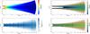 |
Fig. 1 Initial temperature distribution (top left) and logarithmic density distribution (bottom left). The black contour lines show the strength of the initial vertical magnetic field in steps of 0.25 mGauss, starting with 2 mGauss close to 20 AU. Initial resistivity profile with a dust-to-gas mass ratio of 10-2 (top right) and 10-4 (bottom right). Overplotted are contour lines of constant magnetic Reynolds number Rem = csH/η with Rem = 103 and 104. |
2. Methods and model
We solved the non-ideal MHD equations using the PLUTO code (Mignone et al. 2007) with the orbital advection scheme FARGO MHD (Mignone et al. 2012). The equations are
![Mathematical equation: \begin{eqnarray} &&\frac{\partial \rho}{\partial t} + \nabla \cdot (\rho \vec{v}) = 0, \label{eq:MDH_RHO}\\[2pt] && \frac{\partial \rho \vec{v}}{\partial t} + \nabla \cdot \left [ \rho \vec{v} \vec{v}^{\rm T} - \vec{B}\vec{B}^{\rm T} \right ] + \nabla P_{\rm t} = - \rho \nabla \Phi, \label{eq:MDH_MOM} \\[2pt] && \frac{\partial E}{\partial t} \!+\! \nabla \cdot \left [ (E \!+\! P_{\rm t})\vec{v} \!-\! (\vec{v}\cdot\vec{B})\vec{B} \right ] = - \rho \vec{v} \cdot \nabla \Phi \!-\!\nabla \cdot \left [ (\eta \cdot J) \!\times\! B \right ],\, {\rm and} \nonumber\\ \label{eq:MDH_EN} \\[2pt] && \frac{\partial B}{\partial t} + \nabla \times (\vec{v} \times \vec{B}) = -\nabla \times(\eta \cdot J) \label{eq:MDH_MAG} \end{eqnarray}](/articles/aa/full_html/2015/02/aa24693-14/aa24693-14-eq25.png) with the gas density ρ, the velocity vector v, the magnetic field vector B, the total pressure Pt = P + 0.5B2, the gravitational potential Φ, the total energy E = ρϵ + 0.5ρv2 + 0.5B2 with the internal energy ρϵ = P/ (Γ − 1), the current density J = ∇ × B, and the Ohmic resistivity η. We considered Ohmic diffusion. The importance of other magnetic diffusion terms is described in the discussion section. We used a locally isothermal equation of state and fixed Γ = 1.0001. The numerical MHD configuration was taken from Flock et al. (2012b). We use the constrained transport module which conserves ∇·B = 0 to machine precision (Mignone et al. 2007). We used the HLLD Riemann solver (Miyoshi & Kusano 2005). The Courant number was fixed to 0.3.
with the gas density ρ, the velocity vector v, the magnetic field vector B, the total pressure Pt = P + 0.5B2, the gravitational potential Φ, the total energy E = ρϵ + 0.5ρv2 + 0.5B2 with the internal energy ρϵ = P/ (Γ − 1), the current density J = ∇ × B, and the Ohmic resistivity η. We considered Ohmic diffusion. The importance of other magnetic diffusion terms is described in the discussion section. We used a locally isothermal equation of state and fixed Γ = 1.0001. The numerical MHD configuration was taken from Flock et al. (2012b). We use the constrained transport module which conserves ∇·B = 0 to machine precision (Mignone et al. 2007). We used the HLLD Riemann solver (Miyoshi & Kusano 2005). The Courant number was fixed to 0.3.
We continued radial and poloidal gradients of density, pressure, rotation velocity, and resistivity for radial and poloidal boundary conditions. For the radial and poloidal velocity we used a zero gradient with a linear damping of the normal component if it was pointing inward. In the poloidal direction we prevented the density from increasing in the ghost cells. This boundary condition allows for small inward accretion, which slightly reduces the total mass-loss rate.
2.1. Disk model
The initial conditions and parameters of the stellar system are summarized in Table 1 and Fig. 1. The initial gas surface density profile Σ0 follows  (5)with the cylindrical radius R. Temperature and density profiles are in fully hydrostatic equilibrium. The radial domain spans from 20 to 100 AU. We used a logarithmically increasing grid in the radial direction. The vertical extent was Δθ = 0.72 rad. The azimuthal domain spans a full 360°. The local scale height was well resolved with around 20 grid cells in each direction given by the H/R value of about 0.1. A resolution study is presented in Appendix B. The initial vertical magnetic field followed ∝ R-1. We defined the initial magnetic vector potential Aφ = A0 and the magnetic field followed Binit = ∇ × A. The strength of the magnetic field was set with A0 by the condition βmin> 2.0 in the full domain with the plasma beta β = 2P/ (B2). The initial magnetic field strength was about 1 mGauss at 40 AU, which is close to the strength of net vertical field predicted from theoretical models (Okuzumi et al. 2014). The initial resistivity profile was calculated using the chemistry method by Dzyurkevich et al. (2013). The abundances of the main ion, electrons, and charged dust were obtained assuming that the chemistry quickly reaches the charge equilibrium in the presence of small fractal dust (Okuzumi 2009). For the dust chemistry, we considered representative fractal dust aggregates, consisting of 400 monomers of size 0.1 μm1. Such fractal dust particles dominate in the ability to remove free electrons from the surrounding gas (Okuzumi 2009). Metals are frozen out, and the representative ion is HCO+ (Henning & Semenov 2013; Dutrey et al. 2014). We adopted the X-ray ionization rate from Bai & Goodman (2009) (case of 3 keV). The cosmic-ray ionization rate outside of the disk was 5×10-18 s-1. Ionization due to radio-nuclide was 7×10-19 s-1 (D2G / 10-2), where D2G is dust-to-gas mass ratio. We used two different dust-to-gas mass ratios, 10-2 and 10-4, corresponding to models D2G_e-2 and D2G_e-4. The two profiles of the magnetic Reynolds number Rem = csH/η are plotted in Fig. 1 for the fiducial (top right) and the dust-depleted (bottom right) disk model.
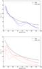 |
Fig. 2 Radial surface density profiles, plotted in steps of 200 inner orbits, from initial (black solid) to final (solid, dotted, dashed, and dashed-dotted) for model D2G_e-2 (blue) and model D2G_e-4 (red). |
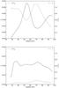 |
Fig. 3 Time-averaged radial profile of the accretion stress α (solid line) and the normalized surface density Σ / Σ0 (dashed line) for models D2G_e-2 (top) and D2G_e-4 (bottom). |
3. Results
In Table 1 we summarize the setup and model parameters. Because of the strong linear MRI phase, which triggers a strong mass outflow, we reset the density to its initial profile after 200 inner orbits. We average the time outputs during the simulation run time after the restart. More details about the linear phase can be found in the Appendix.
The two models quickly established a turbulent state, driven by the MRI. The time-averaged accretion stress was calculated with  (6)The turbulent radial and azimuthal velocities were calculated by subtracting the azimuthally averaged velocities from the total one,
  . This averaging is important because the temperature and consequently, the sound speed cs depend on the radius and height. Along the azimuthal direction, cs is constant and the MRI generated turbulence is self-similar. Model D2G_e-4 shows a strong turbulent state with a time-averaged value of 0.013, while in the fiducial model D2G_e-2, the averaged accretion stress is reduced to 0.003 as a result of the higher resistivity. The variations of the surface density were measured by
  (7)with
  being the surface density averaged over azimuth and ⟨⟩ presenting the space and time average over the full domain and run time. The fluctuations along azimuth are around 4 percent in model D2G_e-2, while they increase to 9 percent in model D2G_e-4. Both values are still low and difficult to resolve with current telescope facilities; see more in Sect. 4. The total surface density over radius evolves distinctly for both models. In Fig. 2 we show the surface density over radius, plotted in steps of 200 inner orbits. In model D2G_e-4 the surface density quickly decreases with time as a result of the strong turbulence. In contrast, model D2G_e-2 shows a gap and jump structure that develop between 50 and 80 AU. The emerging feature is present during the whole simulation time. Time-averaged radial profiles of the accretion stress and the normalized surface density Σ / Σ0 are plotted in Fig. 3. The gap structure in model D2G_e-2 is highly turbulent, while in the jump the turbulence drops by a factor of 2. Radially inward, the higher resistivity starts to dampen the MRI and the accretion stress is reduced. Model D2G_e-4 shows a much stronger accretion stress, nearly constant over radius. Because of the strong turbulence, the surface density in model D2G_e-4 is quickly reduced.
We summarize that we observed the formation of a distinct gap and jump structure in the surface density for our fiducial model with a dust-to-gas mass ratio of 10-2. This structure was anti-correlated with the accretion stress. The gap shows a highly turbulent state, while the jump is less turbulent. The model with a reduced dust amount shows a fully turbulent disk. Here, the strong turbulence leads to a fast removal of the disk.
3.1. Strong zonal-flow structure at the dead-zone outer edge
In this section we investigate the stability of the gap and ring structure by regarding the MRI activity at the dead-zone edge. In Fig. 4 we plot time- (300−500 inner orbits) and space- (± 0.5 H) averaged radial profiles of magnetic pressure B2/ 2, and the normalized surface density 2Σ / Σ0 and deviation of the Keplerian velocity (vφ − vk) /vk. The Elsasser number  for the same time and space average is plotted as background contour color. The structure that emerges in the fiducial model D2G_e-2, Fig. 4 (left), shows very similar characteristics as the classical zonal flow found in local-box simulations (Johansen et al. 2009; Dittrich et al. 2013) and global simulations (Dzyurkevich et al. 2010; Uribe et al. 2011). There is a clear anti-correlation between the magnetic pressure and the surface density profile, also found in local box simulations, compare Fig. 7 by Johansen et al. (2009). The rise in surface density is so strong that the rotation velocity becomes super-Keplerian (see red solid line and annotation). This will stop and even reverse the radial drift of larger particles. At this location, we would expect a high concentration of solid material. Another important feature is the correlation between the Elsasser number with the radial profiles of surface density and magnetic pressure. Inside the gap, the Elsasser number peaks at 0.1, which enables MRI activity (Turner et al. 2007; Okuzumi & Hirose 2011; Flock et al. 2012b). Inside the bump, the Elsasser number is below 0.01, which is clearly not sufficient to enable the MRI. This indicates that the structure is self-sustained because the active part will continue to clear the gas out of the gap. However, the jump in surface density is stable against the MRI. Here, the RWI will eventually grow, while it will try to flatten the jump in surface density. In model D2G_e-2 we observed two cycles of a large vortex formation that lasted for roughly 40 local orbits. The regions around the jump in surface density are MRI turbulent and re-establish the bump, so that the cycle continues (see next section).
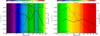 |
Fig. 4 Radial profiles of space and time averaged surface density (solid line), magnetic pressure (dashed line) and deviation of Keplerian rotation (dotted line) for model D2G_e-2 (left) and model D2G_e-4 (right). The background contour color shows the space and time averaged value of the Elsasser number. The red solid line and annotation show the region of super Keplerian rotating gas. At this location, large particles are getting trapped. |
The magnetic fields consist mainly of the toroidal component. In both models, they are dominant in the whole disk with a strength of several mGauss. A full 3D snapshot of the toroidal magnetic field is plotted in Fig. 5 for model D2G_e-2 (left) and model D2G_e-4 (right) after 410 inner orbits. Model D2G_e-4 shows a fully evolved turbulence with small-scale structures in the whole disk. The fiducial model D2G_e-2 shows a smooth field configuration due to the strong resistivity at the inner part, especially inside 50 AU. Both figures show that there is magnetic field accumulation inside the gap and the dead zone. For model D2G_e-4, the Elsasser numbers is well above 0.1 and the MRI operates in the whole disk. Here, we do not observe any gap or jump structure.
3.2. Axisymmetric and non-axisymmetric structures
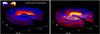 |
Fig. 5 3D plot of the toroidal magnetic field of models D2G_e-2 (left) and D2G_e-4 (right). |
In the fully turbulent model D2G_e-4, the surface density has clear non-axisymmetric structures, which is shown in the surface density maps in Fig. 6 after 400 (top) and 800 (bottom) inner orbits. As shown in Table 1, the strength of these surface density fluctuations are around 10%, which is not high enough to be resolved by current telescopes; see Sect. 4. Here, local enhancements in the surface density with a small spatial extent can reach up to 50%, e.g. in Fig. 6 (bottom left close to 40 AU). The corresponding maps of the vorticity (∇ × v)z at the midplane, Fig. 6 (bottom right), shows that these large-scale structures correlate with a minimum in vorticity. These structures could potentially concentrate particles, similar to concentrations of particles in fully ionized MRI turbulence (Dittrich et al. 2013).
Surface density and vorticity maps of model D2G_e-2 are presented in Fig. 7 after 800 and 1045 inner orbits. Both outputs show the clear gap and following jump in surface density, visible between 50 and 80 AU. The structures are mostly axisymmetric, with small azimuthal fluctuations of about 4%. In this model we observe the formation of a large vortex inside the ring structure at 60 AU (see Fig. 7 bottom), with a surface density enhancement and a corresponding low-vorticity region. The radial extent of the vortex is around 2 scale heights, which corresponds to a radial extent of 10 AU at this location. The azimuthal extent is around 10 H, corresponding to an extent of 50 AU. We tracked two vortices in model D2G_e-2 with similar strength over the full simulation. The first has a lifetime of around 40 local orbits at 60 AU, starting after 350 inner orbits and lasting for 200 inner orbits. The second cycle starts at around 850 and is still present at the final output; see Fig. 7. The vorticity amplitude inside the vortices is around −0.3 [ Ω-1 ], which matches those generated by the RWI (Meheut et al. 2012b, 2013).
We summarize that both models developed surface density enhancements. In the fully turbulent model D2G_e-4 the enhancements are stronger, but with a smaller spatial extent than for model D2G_e-2. In the fiducial model D2G_e-2 we observe a gap followed by a bump in surface density. Inside the bump, vortices are formed by the RWI with a lifetime of around 40 local orbits.
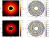 |
Fig. 6 Surface density maps (left) for two different time outputs (400 and 800 inner orbits) for model D2G_e-4 with the corresponding vorticity maps (right). |
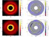 |
Fig. 7 Surface density maps (left) for two different time outputs (800 and 1045 inner orbits) for model D2G_e-2 with the corresponding vorticity maps (right). |
4. Radiative transfer and simulated ALMA maps
The fiducial model showed the generation of a gap and bump in surface density, visible as ring structures located at the outer edge of the dead zone. The decrease and following enhancement of the surface density emerges thanks to a zonal-flow-analog structure, which is located at the transition between the MRI dead and active zone. The model with a reduced dust amount showed fully evolved turbulence. In this section we investigate and compare these two model configurations when observed with ALMA.
4.1. Radiative transfer and ALMA simulations
The radiative transfer (RT)
calculations of the temperature distribution of the dust phase and the corresponding thermal re-emission maps were performed with the Monte Carlo-based 3D continuum RT code MC3D (Wolf et al. 1999; Wolf 2003). The grid structure in the RT simulations was identical to those of the MHD simulations. The radiation source was a T Tauri star in black-body approximation. It is characterized by its luminosity (0.95 L⊙) and effective surface temperature (4000 K).
We focus on the continuum thermal dust emission of disks in face-on orientation. Small dust particles (< 0.25 μm) couple to the gas (Paardekooper & Mellema 2004). Therefore, we derived the spatial dust distribution from the gas density distribution by applying the global dust-to-gas mass ratios listed in Table 1. The dust is composed of 62.5% silicate and 37.5% graphite (optical data by Weingartner & Draine 2001) with a density of the dust material of ρdust = 2.7 g cm-3. The grains are spherical with a grain size distribution following the power-law d n(adust) / d adust ∝ adust− q for a grain size exponent q = 3.5 within the range adust ∈ [0.005 μm,0.25 μm].
We verified that the particles couple to the gas by calculating the Stokes number. The Stokes number in the Epstein regime is 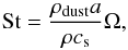 (8)with the orbital frequency Ω, the sound speed
  , the Boltzmann constant kb, the mean molecular weight of μ = 2.353, and the atomic mass unit u. The Epstein regime is valid if the particles are smaller than the mean free path of the gas molecule
  . We estimated the Stokes number for our largest grain size amax = 0.25 μm by assuming a density of ρ = 10-14 g / cm3 and a temperature of 40 K to St(0.25 μm) ∝ 10-4. All the particles up to 0.25 μm are very tightly coupled to the gas. For larger particles of about 100 μm we obtain a value of St(100 μm) ∝ 0.04. For this value we expect strong settling, radial migration, and particle concentration in particular in vortices (Chavanis 2000; Meheut et al. 2012b). A local concentration paired with a higher emission efficiency of these particles in the (sub)mm range would lead to a higher brightness contrast between the gap and its outer edges.
The ALMA observations
were predicted on the basis of simulated thermal dust re-emission. ALMA operates in the wavelength range between 0.3 and 9.3 mm. We considered the complete 12 m-array of 52 (sub)mm-antennas, which can be arranged in different configurations (Brown et al. 2004). We predicted ALMA observations with the CASA 4.2 simulator (Petry & CASA Development Team 2012). It calculates the visibilities in the u-v-plane as sampled by the array configuration, adds noise, and finally reconstructs the image with the CLEAN algorithm. The observing wavelengths listed in Table 2 were selected to optimally suite the atmospheric windows in the (sub)mm range. The bandwidth for the (continuum) ALMA observations is 8 GHz, the selected exposure time amounts to three hours.
Selected wavelengths for the simulated ALMA observations.
With the ALMA sensitivity calculator we estimated the sensitivity that can be achieved for selected wavelengths and spatial resolutions during this time. We considered the influence of thermal and phase noise as summarized in Table 2. The simulated observations were calculated for the reference position (max. height above horizon ≈ 45°) of the Butterfly Star (IRAS 04302+2247, α= 04h33m, δ= +22°53′, J2000) in the Taurus-Auriga star-forming complex. We assumed the following distances of the object: 75 pc (e.g., V4046 Sgr and TW Hya, Rodriguez et al. 2010; Schegerer et al. 2006), 100 pc (e.g., CQ Tau, Guilloteau et al. 2011), 120 pc (e.g., Oph IRS 48, van der Marel et al. 2013), and 140 pc (e.g., HD 169142, Honda et al. 2012).
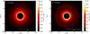 |
Fig. 8 Selected re-emission maps for a wavelength of 1.3 mm and a distance of 100 pc. The maps are calculated for model D2G_e-4 (left) and model D2G_e-2 (right). In these ideal re-emission maps, the turbulent structure in D2G_e-4 and the gap in D2G_e-2 are conserved. |
4.2. Dead-zone edge versus a fully turbulent disk
In this section we compare the re-emission maps and simulated ALMA observations of our fiducial model D2G_e-2 including the dead-zone edge and model D2G_e-4, which is fully turbulent. We focus on a single output after 410 inner orbits because a comparison with other snapshots taken during 100 additional inner orbits did not show any significant differences.
We explored which structures of the (dust) density distribution were conserved in the re-emission maps. Our goal is to identify the structures that are able to distingish between the two models. First we focus on ideal re-emission maps and then consider simulated observations with ALMA.
For the model D2G_e-4 the turbulent structure of the density map is present in the re-emission map (see Fig. 8 left). It is very interesting that model D2G_e-2 shows a ring of reduced brightness at the exact position as the structure in the surface density map (see Fig. 8 right). This gap structure at the same time marks the edge of the dead zone. We note that the total re-emission fluxes are different between the models because of the different total dust mass as a consequence of the different dust-to-gas mass ratios.
The next step was to probe whether it was feasible to trace the structures in these re-emission maps with ALMA. Figure 9 presents the simulated observations for the disk models D2G_e-2 and D2G_e-4 for an object at a distance of 75 pc. Each plot includes the related synthesized beam size, the maximum baseline, and the signal-to-noise ratio (S/N) σ. Furthermore, the figure illustrates the dependence of the observational results on the observing wavelength and atmospheric conditions. It clearly shows that it is possible to trace the gap located at the dead-zone edge in model D2G_e-2 with the distance- and wavelength-dependent significance listed in Table 3. The value of the significance was derived by comparing the (maximum) signal at the outer edge of the gap and the signal at the gap center in the radial brightness profile (see Fig. 10).
Expected significance of gap detections in simulated ALMA observations of model D2G_e-2.
The 871 μm wavelength offers the potential of gap detections with the highest significance (see Table 3). In particular, for objects at a distance of 140 pc a detection of a gap with > 3σ is only possible at this wavelength.
Expected significance of gap detections in simulated ALMA observations of the model Net_e2_Pi in 140 pc distance for different declinations δ of the object at a wavelength of 871 μm.
Additionally, Table 4 shows that the influence of the object position on the significance of a gap detection is small as long as the object reaches a height of more than 40° above the horizon. For model D2G_e-4 the variations of the density are too low (< 10% at the midplane) and limited to a too small area (< 1×1 AU2) to be traced in the simulated ALMA observations. A characteristic ring structure such as the gap in the disk model D2G_e-2 is absent.
However, Fig. 10 also shows that the considered high-angular submillimeter observations alone do not allow one to constrain the origin of the gaps. Giant planets potentially also open gaps in the disk density distribution (Goldreich & Tremaine 1979; Papaloizou & Lin 1984), which create a similar shape of the radial brightness profile, as an example case shows in Fig. 10. The disk with a planet is taken from Ruge et al. (2013) with a planet-to-star mass ratio of 0.001. It also represents a simulated ALMA observation.
Furthermore, we produced scattered-light images of the two disk density models at a reference wavelength of 2.2 μm (K band). They do not show any significant structure in the disk. It is similar to the corresponding scattered-light map of the initial disk setup. Therefore a simple 2D disk model is able to explain the scattered-light appearance of both models. The reason for this is the structure of the photosphere of the disk at the selected wavelength. The disk becomes optically thick for this wavelength already on a surface of the disk where the influence of turbulence and dead-zone edges is too low to be visible. A similar case has been investigated in detail for planet-induced gaps by Ruge et al. (2014).
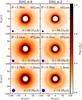 |
Fig. 9 Selected simulated ALMA observations of the two disk models (left column: D2G_e-4, right column: D2G_e-2) at three different wavelengths (top: 441 μm, center: 871 μm, bottom: 1303 μm) at a distance of 75 pc. The longest baselines, synthesized beam sizes, and S/N are plotted into each panel. For comparison, the maps for model D2G_e-4 (left) are scaled with a factor 100. |
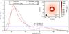 |
Fig. 10 Radial brightness profile of a simulated ALMA map of model D2G_e-2 at a wavelength of 1.3 mm and a distance of 75 pc. Compared to the local flux maximum at 60 AU, the significance of the flux decrease at about 55 AU is 7.7σ. The dashed line shows the radial brightness profile of a disk that is perturbed by a giant planet with a planet-to-star mass ratio of 0.001. The remaining disk parameters correspond to model D2G_e-2. The 10σ level is indicated by the dotted line. The blue line is an auxiliary line that visualizes the maximum flux of the outer disk (red line) at any other location. |
4.3. Consequences of turbulence for gas line observations
CO gas line observations of circumstellar disks frequently find broadened line profiles that cannot be explained by the thermal velocity of the molecules itself (e.g., Guilloteau & Dutrey 1998; Piétu et al. 2007; Qi et al. 2004; Guilloteau et al. 2012). Often, this broadening is considered to be the result of unresolved turbulence in the disk with a velocity component of the molecules toward or away from the observer. It is assumed that the absolute value of this velocity component is on the order of 100 ms-1(e.g., Dartois et al. 2003; Piétu et al. 2007; Hughes et al. 2011). This value can be taken as the FWHM of the velocity distribution in the direction toward the observer. For the turbulent disk model D2G_e-4 with a face-on orientation we obtain Δvz ≈ 127 ms-1, see Fig. 11, top, using the full domain dataset. The velocity distribution is close to a log normal distribution, which is commonly expected for turbulence in this regime (Kritsuk et al. 2011a,b). In the upper disk layers the velocity of the gas component is higher, which leads to a non-negligible influence of the tail end of the distribution (Simon et al. 2011). The mean value of the Gaussian distribution confirms 0.0 ms-1, as expected. In Fig. 11, bottom, we plot the turbulent component of the vertical velocity  for model D2G_e-2, averaged over the azimuth, using a single time output after 410 inner orbits. The dotted lines represent the location of the optical depth unity
  along the vertical direction, with
  and
and  being the line opacity of the molecule, while X is the relative abundance of the molecule. The plot shows that line opacities higher than 10 cm2/ g are more sensitive to the upper disk regions with strong turbulent velocity. For values below 0.1 cm2/ g the optical depth would become optically thin. We note that to obtain an accurate estimate of a molecular line emission, the temperature, the dust properties and the ionization state has to be considered (Henning & Semenov 2013; Dutrey et al. 2014). We summarize that the turbulence in the two disk models is able to create line broadening. Especially the turbulent level of model D2G_e-4 fits currently observed magnitudes.
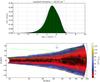 |
Fig. 11 Top: histogram of the vertical velocity component in disk model D2G_e-4. The mean value of the distribution is at zero and the FWHM is ≈ 127 ms-1. The distribution is close to a log-normal distribution. Bottom: contour plot of the vertical RMS velocity component in disk model D2G_e-2. Dotted lines correspond to optical depth τz = 1 lines along the vertical direction for an opacity of κgas = 100,10,1,0.1,cm2/ g. The line of sight of an observer is indicated by an eye sketch. |
5. Discussion
In our models we considered a static resistivity profile. The change of surface density during the simulation will eventually drive a change of ionization of the gas. By including a dynamical resistivity, we expect an enhanced ionization in the gap, which could lead to an even stronger turbulent level in the gap. At the same time, a jump of surface density will decrease the ionization and consequently, the magnetic coupling. A similar study in unstratified simulations that includes the change of ionization in the bump and gap was described in Johansen et al. (2011). Here, they observed a strong pressure bump growing at the dead-zone outer edge. Future studies should include dynamical resistivity to verify the stability of the gap and bump structure.
5.1. Convergence of the MRI
In the Appendix we have performed a resolution study of our models. We compare the results with simulations using half and a quarter of the resolution. The results show that the characteristic radial and vertical profiles of the turbulence converge well, especially for our fiducial model D2G_e-2. We observe the emerging jump in surface density for resolutions down to 10 cells per H. The fully turbulent model D2G_e-4 shows a small increase of turbulence with lower resolution. A recent result that investigated the convergence of the MRI in local-box simulations reported by Bodo et al. (2014) showed a non-convergence of the MRI in zero-net flux stratified disk simulations for resolutions of up to 200 cells per H. A similar result of non-convergence was found in unstratified simulations as well (Fromang & Papaloizou 2007). Here, it was found that the convergence requires fixed diffusion terms (Fromang et al. 2007). The recent result for stratified simulations (Bodo et al. 2014) indicates that there might be similar effects. However, stratified simulations need to include the dynamo effect, which can generate a temporal small net flux that could sustain the turbulence (Davis et al. 2010; Gressel 2010; Flock et al. 2012a). Our global simulations are difficult to compare with high-resolution zero-net flux local-box simulations in the ideal MHD limit. First, we used a vertical net flux field in which convergence is found (Fromang & Papaloizou 2007; Simon et al. 2013). Secondly, we used an explicit magnetic resistivity, which limits the growth of the MRI depending on the strength of the resistivity. We note that we might not be able to resolve very high magnetic Reynolds numbers, especially for values much higher than Rem> 104. The result of our resolution study of model D2G_e-4 could indicate that we still overestimate the level of the turbulence. Flock et al. (2012b) showed a saturation of accretion stress for values above Rem> 3000 but this was tested for a zero-net magnetic field. There, a comparison with ideal MHD and non-ideal MHD simulations using the FARGO scheme showed an effective magnetic Reynolds number of around 5000 for a resolution of H/δx ~ 10. Future simulations should investigate the convergence of the MRI for high magnetic Reynolds numbers in the low Prandtl number regime Pr = ν/η using explicit diffusion terms.
5.2. Ambipolar and Hall term
In this work, we focused on the Ohmic diffusion term. The chosen disk model has a higher surface density than the minimum mass solar nebula (MMSN) model, therefore the Ohmic term is comparable with the ambipolar term at the midplane. However, it is known that magnetic diffusion terms such as ambipolar and Hall diffusion can become the dominant diffusion terms especially in the upper layers of the disk (Wardle 2007; Dzyurkevich et al. 2013; Turner et al. 2014). Recent simulations that included ambipolar diffusion (Bai & Stone 2013) and Hall diffusion (Lesur et al. 2014; Bai 2014) showed a strong laminar stress depending on the field geometry. A similar result, an increase of accretion stress when including Hall diffusion, was seen in multi-fluid global unstratified simulations by O’Keeffe & Downes (2014). In the outer regions, the MRI is expected to produce sufficient accretion stress depending on the net vertical magnetic field even with ambipolar diffusion (Simon et al. 2013). Recent non-ideal MHD local-box simulations in the outer disk regions by Simon & Armitage (2014) observed the generation of zonal flows in the regime dominated by ambipolar diffusion. Future global stratified simulations should investigate the effect of other dissipation terms.
6. Summary and conclusion
We successfully combined non-ideal 3D global MHD simulations of the magneto-rotational instability (MRI) with 3D post-processing radiative transfer methods to predict synthetic ALMA maps. Initial conditions of density and temperature were derived from best-fit models of a generic disk model, which was successfully applied for HH30, CB26, and the Butterfly star. The Ohmic resistivity was calculated consistently from a semi-analytical chemical module. Initial magnetic fields were vertical with a radial profile of 1 /R and a field strength of 1 mGauss at 40 AU. We studied two models with different dust-to-gas mass ratios, 10-2 and 10-4.
-
Both models developed a turbulent state driven by the MRI. Themodel with a dust-to-gas mass ratioof 10-2 included the outer dead-zone edge within the domain, having a laminar inner disk as well as a turbulent region at outer radii. The model with a reduced dust amount was fully turbulent with a time- and space-averaged accretion stress of around 0.01.
-
Close to the dead-zone outer edge, we observed the formation of a large gap and bump structure in the surface density. This structure is similar to a zonal flow, axisymmetrically showing a ring of enhanced surface density. The gap and bump structure was formed due to the response of the MRI onto the change in the density and the Elsasser number. It was sustained during the simulation time of over 1000 inner orbits. The gap showed an increased MRI turbulence compared to the surroundings, with an Elsasser number of around 0.1. The dead-zone and bump structure are less turbulent, with Elsasser numbers below 0.01.
-
The pressure bump at the inner edge of the surface density jump was strong enough to stop the radial drift of solid material. At this location the rotation velocity became slightly super-Keplerian and so prevented the radial migration of large particles.
-
Inside the surface density jump, we observed the formation of vortices by the Rossby wave instability with a lifetime of around 40 local orbits at a location of 60 AU. The vortices show a radial extent of two scale heights (~10 AU) and an azimuthal extent of ten scale heights (~50 AU) with a strength of around −0.3 [ Ω-1 ].
The RT results and simulated ALMA observation showed the difficulty of distinguishing a turbulent from a nearly laminar disk. The turbulent structures in the gas and submicron dust are too small and are impossible to resolve. The same is true for specific time steps of the turbulent disk, which cannot be separated. In addition, there were no traces of turbulence or gaps in the scattered light maps of our models. We highlight that
-
the gap and bump structure produced by the MRI at the dead zoneouter edge can be traced by ALMA;
-
the fully turbulent disk model in face-on orientation is able to create line broadening of the observed size with a FWHM of 127 ms-1.
We note that a distinction between dead-zone edges and planetary gaps remains difficult. Further studies including a particle treatment are necessary to search for possible dust concentration and further asymmetries in disks all the more because our model predicts a concentration of larger particles close to the bump structure. In a follow-up work we will use the existing models and inject particles with different sizes during the simulation runtime by following the particle motion, we will study the radial drift and the concentration to verify with post-processing RT simulations whether it is feasible to trace the observed asymmetries in the disk.
We note that for 2D fractal dust, the size of the monomer is more important than the size of the aggregate to determine the ionization degree (Okuzumi 2009). We chose the monomer size by adopting the values from Wardle (2007). The effect of the monomer size on the ionization profile remains small: changing the monomer size by two orders of magnitude would increase the extent of the dead zone by a factor of 2 (Dzyurkevich et al. 2013).
Acknowledgments
We thank Sebastien Fromang for his great comments and contributions to this work. We also thank Andrea Mignone for his support regarding the PLUTO code and for providing the FARGO MHD method. We thank Wladimir Lyra and Neal Turner for reading and giving comments on the manuscript. Mario Flock is supported by the European Research Council under the European Union’s Seventh Framework Programme (FP7/2007-2013)/ERC Grant agreement No. 258729. Parallel computations have been performed on the IRFU COAST cluster located at CEA IRFU. J.P. Ruge acknowledges the financial support by the German Research Foundation (DFG WO 857/10-1). We thank F. Ober for helpful discussions regarding molecule line observations.
References
- Ataiee, S., Pinilla, P., Zsom, A., et al. 2013, A&A, 553, L3 [NASA ADS] [CrossRef] [EDP Sciences] [Google Scholar]
- Bai, X.-N. 2014, ApJ, 791, 137 [NASA ADS] [CrossRef] [Google Scholar]
- Bai, X.-N., & Goodman, J. 2009, ApJ, 701, 737 [NASA ADS] [CrossRef] [Google Scholar]
- Bai, X.-N., & Stone, J. M. 2013, ApJ, 769, 76 [NASA ADS] [CrossRef] [Google Scholar]
- Balbus, S. A., & Hawley, J. F. 1991, ApJ, 376, 214 [NASA ADS] [CrossRef] [Google Scholar]
- Balbus, S. A., & Hawley, J. F. 1998, Rev. Mod. Phys., 70, 1 [Google Scholar]
- Barge, P., & Sommeria, J. 1995, A&A, 295, L1 [NASA ADS] [Google Scholar]
- Biller, B., Lacour, S., Juhász, A., et al. 2012, ApJ, 753, L38 [NASA ADS] [CrossRef] [Google Scholar]
- Birnstiel, T., Dullemond, C. P., & Pinilla, P. 2013, A&A, 550, L8 [NASA ADS] [CrossRef] [EDP Sciences] [Google Scholar]
- Blaes, O. M., & Balbus, S. A. 1994, ApJ, 421, 163 [NASA ADS] [CrossRef] [Google Scholar]
- Bodo, G., Cattaneo, F., Mignone, A., & Rossi, P. 2014, ApJ, 787, L13 [NASA ADS] [CrossRef] [Google Scholar]
- Brown, R. L., Wild, W., & Cunningham, C. 2004, Adv. Space Res., 34, 555 [NASA ADS] [CrossRef] [Google Scholar]
- Brown, J. M., Blake, G. A., Qi, C., et al. 2009, ApJ, 704, 496 [NASA ADS] [CrossRef] [Google Scholar]
- Casassus, S., van der Plas, G., Perez, MS., et al. 2013, Nature, 493, 191 [NASA ADS] [CrossRef] [Google Scholar]
- Chavanis, P. H. 2000, A&A, 356, 1089 [NASA ADS] [Google Scholar]
- Close, L. M., Follette, K. B., Males, J. R., et al. 2014, ApJ, 781, L30 [NASA ADS] [CrossRef] [Google Scholar]
- Dartois, E., Dutrey, A., & Guilloteau, S. 2003, A&A, 399, 773 [NASA ADS] [CrossRef] [EDP Sciences] [Google Scholar]
- Davis, S. W., Stone, J. M., & Pessah, M. E. 2010, ApJ, 713, 52 [NASA ADS] [CrossRef] [Google Scholar]
- de Val-Borro, M., Artymowicz, P., D’Angelo, G., & Peplinski, A. 2007, A&A, 471, 1043 [NASA ADS] [CrossRef] [EDP Sciences] [Google Scholar]
- Dittrich, K., Klahr, H., & Johansen, A. 2013, ApJ, 763, 117 [NASA ADS] [CrossRef] [Google Scholar]
- Dutrey, A., Semenov, D., Chapillon, E., et al. 2014, in Protostars and Planets VI (University of Arizona Press) [arXiv:1402.3503] [Google Scholar]
- Dzyurkevich, N., Flock, M., Turner, N. J., Klahr, H., & Henning, T. 2010, A&A, 515, A70 [NASA ADS] [CrossRef] [EDP Sciences] [Google Scholar]
- Dzyurkevich, N., Turner, N. J., Henning, T., & Kley, W. 2013, ApJ, 765, 114 [NASA ADS] [CrossRef] [Google Scholar]
- Faure, J., Fromang, S., & Latter, H. 2014, A&A, 564, A22 [NASA ADS] [CrossRef] [EDP Sciences] [Google Scholar]
- Flock, M., Dzyurkevich, N., Klahr, H., & Mignone, A. 2010, A&A, 516, A26 [NASA ADS] [CrossRef] [EDP Sciences] [Google Scholar]
- Flock, M., Dzyurkevich, N., Klahr, H., Turner, N., & Henning, T. 2012a, ApJ, 744, 144 [NASA ADS] [CrossRef] [Google Scholar]
- Flock, M., Henning, T., & Klahr, H. 2012b, ApJ, 761, 95 [NASA ADS] [CrossRef] [Google Scholar]
- Fromang, S., & Papaloizou, J. 2007, A&A, 476, 1113 [NASA ADS] [CrossRef] [EDP Sciences] [Google Scholar]
- Fromang, S., Papaloizou, J., Lesur, G., & Heinemann, T. 2007, A&A, 476, 1123 [NASA ADS] [CrossRef] [EDP Sciences] [Google Scholar]
- Fukagawa, M., Tsukagoshi, T., Momose, M., et al. 2013, PASJ, 65, L14 [NASA ADS] [CrossRef] [Google Scholar]
- Goldreich, P., & Tremaine, S. 1979, ApJ, 233, 857 [NASA ADS] [CrossRef] [MathSciNet] [Google Scholar]
- Gräfe, C., Wolf, S., Guilloteau, S., et al. 2013, A&A, 553, A69 [NASA ADS] [CrossRef] [EDP Sciences] [Google Scholar]
- Gressel, O. 2010, MNRAS, 405, 41 [NASA ADS] [CrossRef] [Google Scholar]
- Guilloteau, S., & Dutrey, A. 1998, A&A, 339, 467 [NASA ADS] [Google Scholar]
- Guilloteau, S., Dutrey, A., Piétu, V., & Boehler, Y. 2011, A&A, 529, A105 [NASA ADS] [CrossRef] [EDP Sciences] [Google Scholar]
- Guilloteau, S., Dutrey, A., Wakelam, V., et al. 2012, A&A, 548, A70 [NASA ADS] [CrossRef] [EDP Sciences] [Google Scholar]
- Henning, T., & Semenov, D. 2013, Chem. Rev., 113, 9016 [Google Scholar]
- Honda, M., Maaskant, K., Okamoto, Y. K., et al. 2012, ApJ, 752, 143 [NASA ADS] [CrossRef] [Google Scholar]
- Hughes, A. M., Wilner, D. J., Andrews, S. M., Qi, C., & Hogerheijde, M. R. 2011, ApJ, 727, 85 [NASA ADS] [CrossRef] [Google Scholar]
- Inaba, S., & Barge, P. 2006, ApJ, 649, 415 [NASA ADS] [CrossRef] [EDP Sciences] [Google Scholar]
- Isella, A., Pérez, L. M., Carpenter, J. M., et al. 2013, ApJ, 775, 30 [NASA ADS] [CrossRef] [MathSciNet] [Google Scholar]
- Johansen, A., Andersen, A. C., & Brandenburg, A. 2004, A&A, 417, 361 [NASA ADS] [CrossRef] [EDP Sciences] [Google Scholar]
- Johansen, A., Youdin, A., & Klahr, H. 2009, ApJ, 697, 1269 [NASA ADS] [CrossRef] [Google Scholar]
- Johansen, A., Kato, M., & Sano, T. 2011, in IAU Symp. 274, eds. A. Bonanno, E. de Gouveia Dal Pino, & A. G. Kosovichev, 50 [Google Scholar]
- Klahr, H. H., & Henning, T. 1997, Icarus, 128, 213 [NASA ADS] [CrossRef] [Google Scholar]
- Koller, J., Li, H., & Lin, D. N. C. 2003, ApJ, 596, L91 [NASA ADS] [CrossRef] [Google Scholar]
- Kritsuk, A. G., Norman, M. L., & Wagner, R. 2011a, ApJ, 727, L20 [NASA ADS] [CrossRef] [Google Scholar]
- Kritsuk, A. G., Ustyugov, S. D., & Norman, M. L. 2011b, in Computational Star Formation, eds. J. Alves, B. G. Elmegreen, J. M. Girart, & V. Trimble, IAU Symp., 270, 179 [Google Scholar]
- Lesur, G., Kunz, M. W., & Fromang, S. 2014, A&A, 566, A56 [NASA ADS] [CrossRef] [EDP Sciences] [Google Scholar]
- Lin, M.-K. 2012, ApJ, 754, 21 [Google Scholar]
- Liu, Y., Madlener, D., Wolf, S., Wang, H., & Ruge, J. P. 2012, A&A, 546, A7 [NASA ADS] [CrossRef] [EDP Sciences] [Google Scholar]
- Lyra, W., & Lin, M.-K. 2013, ApJ, 775, 17 [NASA ADS] [CrossRef] [Google Scholar]
- Lyra, W., & Mac Low, M.-M. 2012, ApJ, 756, 62 [NASA ADS] [CrossRef] [Google Scholar]
- Lyra, W., Johansen, A., Klahr, H., & Piskunov, N. 2008, A&A, 491, L41 [NASA ADS] [CrossRef] [EDP Sciences] [Google Scholar]
- Lyra, W., Johansen, A., Klahr, H., & Piskunov, N. 2009a, A&A, 493, 1125 [NASA ADS] [CrossRef] [EDP Sciences] [Google Scholar]
- Lyra, W., Johansen, A., Zsom, A., Klahr, H., & Piskunov, N. 2009b, A&A, 497, 869 [NASA ADS] [CrossRef] [EDP Sciences] [Google Scholar]
- Lyra, W., Turner, N., & McNally, C. 2015, A&A, 574, A10 [NASA ADS] [CrossRef] [EDP Sciences] [Google Scholar]
- Madlener, D., Wolf, S., Dutrey, A., & Guilloteau, S. 2012, A&A, 543, A81 [NASA ADS] [CrossRef] [EDP Sciences] [Google Scholar]
- Meheut, H., Casse, F., Varniere, P., & Tagger, M. 2010, A&A, 516, A31 [NASA ADS] [CrossRef] [EDP Sciences] [Google Scholar]
- Meheut, H., Keppens, R., Casse, F., & Benz, W. 2012a, A&A, 542, A9 [Google Scholar]
- Meheut, H., Meliani, Z., Varniere, P., & Benz, W. 2012b, A&A, 545, A134 [NASA ADS] [CrossRef] [EDP Sciences] [Google Scholar]
- Meheut, H., Lovelace, R. V. E., & Lai, D. 2013, MNRAS, 430, 1988 [NASA ADS] [CrossRef] [Google Scholar]
- Mignone, A., Bodo, G., Massaglia, S., et al. 2007, ApJS, 170, 228 [Google Scholar]
- Mignone, A., Flock, M., Stute, M., Kolb, S. M., & Muscianisi, G. 2012, A&A, 545, A152 [NASA ADS] [CrossRef] [EDP Sciences] [Google Scholar]
- Miyoshi, T., & Kusano, K. 2005, J. Comput. Phys., 208, 315 [NASA ADS] [CrossRef] [Google Scholar]
- O’Keeffe, W., & Downes, T. P. 2014, MNRAS, 441, 571 [NASA ADS] [CrossRef] [Google Scholar]
- Okuzumi, S. 2009, ApJ, 698, 1122 [NASA ADS] [CrossRef] [Google Scholar]
- Okuzumi, S., & Hirose, S. 2011, ApJ, 742, 65 [NASA ADS] [CrossRef] [Google Scholar]
- Okuzumi, S., Takeuchi, T., & Muto, T. 2014, ApJ, 785, 127 [NASA ADS] [CrossRef] [Google Scholar]
- Paardekooper, S.-J., & Mellema, G. 2004, A&A, 425, L9 [NASA ADS] [CrossRef] [EDP Sciences] [Google Scholar]
- Papaloizou, J., & Lin, D. N. C. 1984, ApJ, 285, 818 [NASA ADS] [CrossRef] [Google Scholar]
- Pérez, L. M., Isella, A., Carpenter, J. M., & Chandler, C. J. 2014, ApJ, 783, L13 [NASA ADS] [CrossRef] [Google Scholar]
- Petry, D., & CASA Development Team 2012, in Astronomical Data Analysis Software and Systems XXI, eds. P. Ballester, D. Egret, & N. P. F. Lorente, ASP Conf. Ser., 461, 849 [Google Scholar]
- Piétu, V., Dutrey, A., & Guilloteau, S. 2007, A&A, 467, 163 [NASA ADS] [CrossRef] [EDP Sciences] [Google Scholar]
- Qi, C., Ho, P. T. P., Wilner, D. J., et al. 2004, ApJ, 616, L11 [NASA ADS] [CrossRef] [Google Scholar]
- Regály, Z., Juhász, A., Sándor, Z., & Dullemond, C. P. 2012, MNRAS, 419, 1701 [NASA ADS] [CrossRef] [Google Scholar]
- Rodriguez, D. R., Kastner, J. H., Wilner, D., & Qi, C. 2010, ApJ, 720, 1684 [NASA ADS] [CrossRef] [Google Scholar]
- Ruge, J. P., Wolf, S., Uribe, A. L., & Klahr, H. H. 2013, A&A, 549, A97 [NASA ADS] [CrossRef] [EDP Sciences] [Google Scholar]
- Ruge, J. P., Wolf, S., Uribe, A. L., & Klahr, H. H. 2014, A&A, 572, L2 [NASA ADS] [CrossRef] [EDP Sciences] [Google Scholar]
- Sano, T., & Stone, J. M. 2002, ApJ, 570, 314 [NASA ADS] [CrossRef] [Google Scholar]
- Sauter, J., Wolf, S., Launhardt, R., et al. 2009, A&A, 505, 1167 [NASA ADS] [CrossRef] [EDP Sciences] [Google Scholar]
- Schegerer, A., Wolf, S., Voshchinnikov, N. V., Przygodda, F., & Kessler-Silacci, J. E. 2006, A&A, 456, 535 [NASA ADS] [CrossRef] [EDP Sciences] [Google Scholar]
- Schegerer, A. A., Wolf, S., Ratzka, T., & Leinert, C. 2008, A&A, 478, 779 [NASA ADS] [CrossRef] [EDP Sciences] [Google Scholar]
- Schegerer, A. A., Wolf, S., Hummel, C. A., Quanz, S. P., & Richichi, A. 2009, A&A, 502, 367 [NASA ADS] [CrossRef] [EDP Sciences] [Google Scholar]
- Simon, J. B., & Armitage, P. J. 2014, ApJ, 784, 15 [NASA ADS] [CrossRef] [Google Scholar]
- Simon, J. B., Armitage, P. J., & Beckwith, K. 2011, ApJ, 743, 17 [NASA ADS] [CrossRef] [Google Scholar]
- Simon, J. B., Bai, X.-N., Armitage, P. J., Stone, J. M., & Beckwith, K. 2013, ApJ, 775, 73 [NASA ADS] [CrossRef] [Google Scholar]
- Turner, N. J., Sano, T., & Dziourkevitch, N. 2007, ApJ, 659, 729 [NASA ADS] [CrossRef] [Google Scholar]
- Turner, N. J., Carballido, A., & Sano, T. 2010, ApJ, 708, 188 [NASA ADS] [CrossRef] [Google Scholar]
- Turner, N. J., Fromang, S., Gammie, C., et al. 2014, in Protostars and Planets VI (University of Arizona Press) [arXiv:1401.7306] [Google Scholar]
- Uribe, A. L., Klahr, H., Flock, M., & Henning, T. 2011, ApJ, 736, 85 [NASA ADS] [CrossRef] [Google Scholar]
- van der Marel, N., van Dishoeck, E. F., Bruderer, S., et al. 2013, Science, 340, 1199 [NASA ADS] [CrossRef] [PubMed] [Google Scholar]
- Varnière, P., & Tagger, M. 2006, A&A, 446, L13 [NASA ADS] [CrossRef] [EDP Sciences] [Google Scholar]
- Wardle, M. 2007, Ap&SS, 311, 35 [NASA ADS] [CrossRef] [Google Scholar]
- Weingartner, J. C., & Draine, B. T. 2001, ApJ, 548, 296 [NASA ADS] [CrossRef] [Google Scholar]
- Wolf, S. 2003, Comput. Phys. Commun., 150, 99 [NASA ADS] [CrossRef] [Google Scholar]
- Wolf, S., & Klahr, H. 2002, ApJ, 578, L79 [NASA ADS] [CrossRef] [Google Scholar]
- Wolf, S., Henning, T., & Stecklum, B. 1999, A&A, 349, 839 [NASA ADS] [Google Scholar]
- Wolf, S., Padgett, D. L., & Stapelfeldt, K. R. 2003, ApJ, 588, 373 [NASA ADS] [CrossRef] [Google Scholar]
- Wolf, S., Schegerer, A., Beuther, H., Padgett, D. L., & Stapelfeldt, K. R. 2008, ApJ, 674, L101 [NASA ADS] [CrossRef] [Google Scholar]
- Zhu, Z., Stone, J. M., Rafikov, R. R., & Bai, X.-N. 2014, ApJ, 785, 122 [NASA ADS] [CrossRef] [Google Scholar]
Appendix A: Initial phase
The model parameters are summarized in Table A.1. All runs show a strong linear MRI phase due to the net vertical field. The time-averaged α values during the first 300 inner orbits reach 0.038 for model D2G_e-2I and 0.054 for model D2G_e-4I, which will lead to a strong mass loss in both simulations. A snapshot of the turbulent radial magnetic field is shown in Fig. A.1 after 100 inner orbits for each model. The turbulent magnetic fields reach a strength of several mGauss. Model D2G_e-2I shows a strongly damped inner midplane region, Fig. A.1, top. Between 50 and 60 AU a transition from this laminar dead-zone to a turbulent active zone is recognizable. We note that the midplane region is damped, while the upper layers are still active. To continue the simulations, we reestablished the initial state of density and pressure and extended the azimuthal domain to full 2π. We restarted the simulations from the initial conditions, but replaced the initial magnetic fields with the fields obtained after 200 inner orbits. This prevented the strong rise of turbulent activity while at the same time a turbulent steady state was reached quickly. The plasma beta  at 40 AU for the initial magnetic field was around 2200 (which corresponds to 1 mGauss), which led to a strong turbulent evolution. After 200 inner orbits, the large radial mass-loss also led to a reduction of the vertical magnetic flux. When we reset the density and pressure, the plasma beta for the vertical field at the midplane at 40 AU increased to around 44 000.
Model name, resolution, domain size, dust-to-gas mass ratio, and averaged accretion stress.
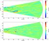 |
Fig. A.1 Snapshots of the turbulent radial magnetic field in the R-Z plane after 100 inner orbits for model D2G_e-2I (top) and model D2G_e-4I (bottom). |
Appendix B: Resolution study
In the following section, we perform a resolution study to determine the robustness of our results. We included four additional simulations, two for each dust-to-gas mass ratio, with half and a quarter of the resolution. In Fig. B.1 we compare the radial and vertical profiles of accretion stress for all different models, see Table B.1. To calculate the results, we used the same time average, between 300 and 500 inner orbits. We used exactly the same restart technique for all models. The vertical profiles were taken from the middle of the domain. Our fiducial disk model with a dust-to-gas mass ratio of 10-2 shows a very good convergence even with only five grid cells per scale height. This result was surprising because we expected to resolve the fastest growing mode of the MRI with eight cells per H or more (Flock et al. 2010). This could indicate that the FARGO MHD method is able to resolve the fastest growing modes with slightly fewer cells. The models with a reduced dust amount show a small decrease in the accretion stress with higher resolution. We explain this by the fact that only the largest and strongest modes are resolved in the low-resolution runs. In general, small-scale turbulence can have a dampening effect on the larger scales. We observe the emerging jump in surface density for resolutions down to 10 cells per H. The lowest resolution has around five cells per H, and this model is unable to develope the gap and bump structure. In the following, we check for the low-resolution model D2G_e-2R10 how the gap and jump structure appears when observed with ALMA.
Model name, resolution, and grid cells per H.
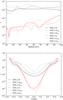 |
Fig. B.1 Radial (top) and vertical (bottom) profile of the accretion stress α for three different resolutions and two different dust-to-gas mass ratios averaged over 200 inner orbits (300 to 500 inner orbits). Here, the cylindrical height Z is given by Z = Rmidsinθ with Rmid = 60 AU. |
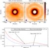 |
Fig. B.2 Top: selected simulated ALMA observations of the two disk models (left column: D2G_e-4R10, right column: D2G_e-2R10 at a wavelength of 871 μm and a distance of 75 pc. For comparison, the maps for model D2G_e-4R10 (left) are again scaled with a factor 100. Bottom: radial brightness profile of a simulated ALMA map of the two models. |
The radiative transfer results for the models of reduced resolution achieve the same precision in calculating of the temperature distribution of the disk and the resulting re-emission maps as the high-resolution maps (see Sect. 4). For the disk model D2G_e-4 it is not possible to distinguish the radiative transfer results for the different resolutions of the MHD simulation. We present this result through a simulated ALMA observation shown in Fig. B.2 (top left), which is the counter piece to the ALMA simulation of the high-resolution case shown in Fig. 9 (mid-left). The re-emission maps for the disk simulation D2G_e-2R10 again show a ring of reduced brightness at the exact position of this structure in the surface density map. In the radial brightness profile as well as in the surface density map, the location of the gap is about 10 AU more distant from the disk center than for the high-resolution map (see Fig. B.2, bottom). This gap is detectable with ALMA; for example, we present a simulated ALMA observation at a wavelength of 871 μm for a disk at 75 pc distance in Fig. B.2, top. Finally, ALMA is able to measure the position and width of the gap on the order of the beam size.
All Tables
Model name, resolution, domain size, dust-to-gas mass ratio, run time, averaged accretion stress, and averaged azimuthal surface density variations (top). Disk and stellar parameters (bottom).
Expected significance of gap detections in simulated ALMA observations of model D2G_e-2.
Expected significance of gap detections in simulated ALMA observations of the model Net_e2_Pi in 140 pc distance for different declinations δ of the object at a wavelength of 871 μm.
Model name, resolution, domain size, dust-to-gas mass ratio, and averaged accretion stress.
All Figures
|
Fig. 1 Initial temperature distribution (top left) and logarithmic density distribution (bottom left). The black contour lines show the strength of the initial vertical magnetic field in steps of 0.25 mGauss, starting with 2 mGauss close to 20 AU. Initial resistivity profile with a dust-to-gas mass ratio of 10-2 (top right) and 10-4 (bottom right). Overplotted are contour lines of constant magnetic Reynolds number Rem = csH/η with Rem = 103 and 104. |
| In the text | |
|
Fig. 2 Radial surface density profiles, plotted in steps of 200 inner orbits, from initial (black solid) to final (solid, dotted, dashed, and dashed-dotted) for model D2G_e-2 (blue) and model D2G_e-4 (red). |
| In the text | |
|
Fig. 3 Time-averaged radial profile of the accretion stress α (solid line) and the normalized surface density Σ / Σ0 (dashed line) for models D2G_e-2 (top) and D2G_e-4 (bottom). |
| In the text | |
|
Fig. 4 Radial profiles of space and time averaged surface density (solid line), magnetic pressure (dashed line) and deviation of Keplerian rotation (dotted line) for model D2G_e-2 (left) and model D2G_e-4 (right). The background contour color shows the space and time averaged value of the Elsasser number. The red solid line and annotation show the region of super Keplerian rotating gas. At this location, large particles are getting trapped. |
| In the text | |
|
Fig. 5 3D plot of the toroidal magnetic field of models D2G_e-2 (left) and D2G_e-4 (right). |
| In the text | |
|
Fig. 6 Surface density maps (left) for two different time outputs (400 and 800 inner orbits) for model D2G_e-4 with the corresponding vorticity maps (right). |
| In the text | |
|
Fig. 7 Surface density maps (left) for two different time outputs (800 and 1045 inner orbits) for model D2G_e-2 with the corresponding vorticity maps (right). |
| In the text | |
|
Fig. 8 Selected re-emission maps for a wavelength of 1.3 mm and a distance of 100 pc. The maps are calculated for model D2G_e-4 (left) and model D2G_e-2 (right). In these ideal re-emission maps, the turbulent structure in D2G_e-4 and the gap in D2G_e-2 are conserved. |
| In the text | |
|
Fig. 9 Selected simulated ALMA observations of the two disk models (left column: D2G_e-4, right column: D2G_e-2) at three different wavelengths (top: 441 μm, center: 871 μm, bottom: 1303 μm) at a distance of 75 pc. The longest baselines, synthesized beam sizes, and S/N are plotted into each panel. For comparison, the maps for model D2G_e-4 (left) are scaled with a factor 100. |
| In the text | |
|
Fig. 10 Radial brightness profile of a simulated ALMA map of model D2G_e-2 at a wavelength of 1.3 mm and a distance of 75 pc. Compared to the local flux maximum at 60 AU, the significance of the flux decrease at about 55 AU is 7.7σ. The dashed line shows the radial brightness profile of a disk that is perturbed by a giant planet with a planet-to-star mass ratio of 0.001. The remaining disk parameters correspond to model D2G_e-2. The 10σ level is indicated by the dotted line. The blue line is an auxiliary line that visualizes the maximum flux of the outer disk (red line) at any other location. |
| In the text | |
|
Fig. 11 Top: histogram of the vertical velocity component in disk model D2G_e-4. The mean value of the distribution is at zero and the FWHM is ≈ 127 ms-1. The distribution is close to a log-normal distribution. Bottom: contour plot of the vertical RMS velocity component in disk model D2G_e-2. Dotted lines correspond to optical depth τz = 1 lines along the vertical direction for an opacity of κgas = 100,10,1,0.1,cm2/ g. The line of sight of an observer is indicated by an eye sketch. |
| In the text | |
|
Fig. A.1 Snapshots of the turbulent radial magnetic field in the R-Z plane after 100 inner orbits for model D2G_e-2I (top) and model D2G_e-4I (bottom). |
| In the text | |
|
Fig. B.1 Radial (top) and vertical (bottom) profile of the accretion stress α for three different resolutions and two different dust-to-gas mass ratios averaged over 200 inner orbits (300 to 500 inner orbits). Here, the cylindrical height Z is given by Z = Rmidsinθ with Rmid = 60 AU. |
| In the text | |
|
Fig. B.2 Top: selected simulated ALMA observations of the two disk models (left column: D2G_e-4R10, right column: D2G_e-2R10 at a wavelength of 871 μm and a distance of 75 pc. For comparison, the maps for model D2G_e-4R10 (left) are again scaled with a factor 100. Bottom: radial brightness profile of a simulated ALMA map of the two models. |
| In the text | |
Current usage metrics show cumulative count of Article Views (full-text article views including HTML views, PDF and ePub downloads, according to the available data) and Abstracts Views on Vision4Press platform.
Data correspond to usage on the plateform after 2015. The current usage metrics is available 48-96 hours after online publication and is updated daily on week days.
Initial download of the metrics may take a while.