| Issue |
A&A
Volume 574, February 2015
|
|
|---|---|---|
| Article Number | A127 | |
| Number of page(s) | 33 | |
| Section | Extragalactic astronomy | |
| DOI | https://doi.org/10.1051/0004-6361/201322805 | |
| Published online | 05 February 2015 | |
Diagnostics of the molecular component of photon-dominated regions with mechanical heating
II. Line intensities and ratios ⋆,⋆⋆
1
Leiden Observatory, Leiden University,
PO Box 9513
2300 RA,
Leiden,
The Netherlands
e-mail:
This email address is being protected from spambots. You need JavaScript enabled to view it.
2
Kapteyn Astronomical Institute, PO Box 800, 9700 AV
Groningen, The
Netherlands
Received: 4 October 2013
Accepted: 10 April 2014
Abstract
CO observations in active galactic nuclei and starbursts reveal high kinetic temperatures. Those environments are thought to be very turbulent due to dynamic phenomena, such as outflows and high supernova rates. We investigate the effect of mechanical heating on atomic fine-structure and molecular lines and on their ratios. We try to use those ratios as a diagnostic to constrain the amount of mechanical heating in an object and also study its significance on estimating the H2 mass. Equilibrium photodissociation models (PDRs hereafter) were used to compute the thermal and chemical balance for the clouds. The equilibria were solved for numerically using the optimized version of the Leiden PDR-XDR code. Large velocity-gradient calculations were done as post-processing on the output of the PDR models using RADEX. High-J CO line ratios are very sensitive to mechanical heating (Γmech hereafter). These emission becomes at least one order of magnitude brighter in clouds with n ~ 105 cm-3 and a star formation rate of 1 M⊙ yr-1 (corresponding to Γmech = 2 × 10-19 erg cm-3 s-1). The emission of low-J CO lines is not as sensitive to Γmech, but they do become brighter in response to Γmech. Generally, for all of the lines we considered, Γmech increases excitation temperatures and decreases the optical depth at the line centre. Hence line ratios are also affected, strongly in some cases. Ratios involving HCN are a good diagnostic for Γmech, where the HCN(1–0)/CO(1–0) increases from 0.06 to 0.25, and the HCN(1–0)/HCO+(1–0) increase from 0.15 to 0.5 for amounts of Γmech that are equivalent to 5% of the surface heating rate. Both ratios increase to more than 1 for higher Γmech, as opposed to being much less than unity in pure PDRs. The first major conclusion is that low-J to high-J intensity ratios will yield a good estimate of the mechanical heating rate (as opposed to only low-J ratios). The second one is that the mechanical heating rate should be taken into account when determing AV or, equivalently, NH, and consequently the cloud mass. Ignoring Γmech will also lead to large errors in density and radiation field estimates.
Key words: galaxies: ISM / photon-dominated region / turbulence / ISM: molecules / ISM: clouds
Appendices are available in electronic form at http://www.aanda.org
The data used to generate all the grids are only available at the CDS via anonymous ftp to cdsarc.u-strasbg.fr (130.79.128.5) or via http://cdsarc.u-strasbg.fr/viz-bin/qcat?J/A+A/574/A127
© ESO, 2015
1. Introduction
The study of molecular gas in external galaxies dates back to the mid-seventies, with the detection of ground-state emission from CO (the most abundant molecules after hydrogen) in a small number of bright nearby galaxies. At present, observations CO and many other molecules exist for a very large number of galaxies, near and far. It is important to be able to interpret the emission in the various lines from those galaxies, since that gives us insight into the physics dominating the interstellar medium (ISM) in the star forming regions of these extra-galactic sources.
For decades, line observations had to be done from the ground in a frequency range limited by atmospheric opacity, so that for most molecular species only the low transitions were accessible. Level transitions at higher rest frame frequencies were only possible for distant galaxies for which the high-frequency lines were red-shifted into atmospheric windows accessible from the ground. In the past few years, the Herschel Space Observatory (Pilbratt et al. 2010) operating outside the Earth’s atmosphere has provided direct observations of spectral lines at frequencies hitherto impossible or hard to access.
By way of example we mention the determination of extensive 12CO rotational transitions ladder in galaxies such as M 82 (Loenen et al. 2010; Panuzzo et al. 2010; Kamenetzky et al. 2012) and Mrk231 (van der Werf et al. 2010; González-Alfonso et al. 2012). Herschel ran out of coolant in April 2013, but at about the same time, the Atacama Large Millimeter Array (ALMA) became operational. With ALMA, a large fraction of the important submillimeter spectrum is still accessible, at vastly superior resolution and sensitivity, allowing detection and measurement of diagnostic molecular line transitions largely out of reach until then.
Conducting detailed studies of the physical properties of the molecular gas of close-by star-forming galaxies involves a challenging inversion problem, where resultant line intensities are used to constrain gas densities, molecular content, kinetic temperatures and the nature and strengths of the radiation field exciting the gas. In order to solve this problem, it is necessary to get a clearer understanding of the underlying physics and phenomena characterizing specific regions such as galaxy centres, including our own.
A good starting point to analyse molecular gas emission is to apply the so-called large-velocity-gradient (LVG) models (Sobolev 1960). This assumes an escape probability formalism for photons in different geometries, which simplifies solving for the radiative transfer significantly. LVG models have been widely used by the ISM community with some other basic assumptions to estimate the molecular density of the gas, species abundances and the kinetic temperature (Henkel et al. 1983; Jansen et al. 1994; Hogerheijde & van der Tak 2000; Schöier et al. 2005; Krumholz 2014, among others). These models provide only an insight into the physical and chemical properties of the clouds, and the actual nature of the source of energy cannot be determined using those LVG models (see for example Israel 2009a,b). The next level of sophistication over LVG modelling involves the application of photon-dominated region (PDR) models (Ferland et al. 1998; Hollenbach & Tielens 1999; Le Petit et al. 2006; Röllig et al. 2007; Bisbas et al. 2012). These models self-consistently solve for the thermal and chemical structure of clouds irradiated by UV photons.
In PDRs, energy sources other than UV photons could dominate the thermal and chemical balance. In the vicinity of an active galactic nucleus (AGN), PDR models can be augmented by models for X-ray dominated region (XDRs Maloney et al. 1996; Bradford et al. 2003; Meijerink & Spaans 2005; Papadopoulos et al. 2011; Bayet et al. 2011; Meijerink et al. 2011).
In both these models, the underlying assumption is that the thermal balance is dominated by radiation. The physical situation in galaxy centres, starbursts and dense cores (Pineda et al. 2010) is, however, more complicated. There are other processes, such as mechanical feedback that may also excite the gas mechanically (Loenen et al. 2008; Ossenkopf & Mac Low 2002; Ossenkopf 2002; Kazandjian et al. 2012).
Although these models are much more sophisticated than LVG models, a simplified comparison of many PDR codes1 (Röllig et al. 2007) has shown that they shed a statistical view on the underlying processes. This is particularly true in the transition zone from atomic to molecular gas, where an order of magnitude difference between the various quantities compared in the models is not uncommon. Such discrepancies are mainly due to the uncertainties in the chemical reaction constants, which in turn influence the reaction rates, abundances and thermal balance (Vasyunin et al. 2004). In addition to those uncertainties observations of extra-galactic sources have spatial resolution limitations. For example the resolution of Herschel for the nucleus of NGC 253 is of the order of 1 kpc. The surface area covered by such a beam size contains a large number of clouds. In modelling the nucleus of such galaxies one might need to consider two or more PDRs simultaneously. Although considering more than one PDR component improves the fits significantly, the increased number of free parameters usually has a negative impact on to the statistical significance of those fits. This is particularly valid whenever the number of lines being fitted is low.
Here we follow the modelling of Paper I (Kazandjian et al. 2012) where we studied the effect of mechanical heating (Γmech) by considering its impact on the thermal and chemical structure (abundances, column densities and column density ratios of species) of PDRs. Hence our basic modelling premise will be the same in this paper. Namely, an 1D semi-infinite plane-parallel geometry is adopted. It is assumed that the slab is illuminated with a far-ultraviolet (FUV) source from one side. Another major assumption is that the clouds are in an equilibrium state. Since equilibrium is assumed, we consider a simplified recipe in accounting for mechanical feedback. For simplicity the contribution of mechanical heating to the total heating budget, is added in an ad hoc fashion uniformly throughout the cloud.
Our approximation of the effect of mechanical heating by a single homogeneous heating term is a simplification. In practice, the mechanical energy which could be liberated by supernova events or gas outflows, is deposited locally in shock fronts. In these fronts, which are the interaction surfaces between high speed flows and the ambient medium, the energy is not necessarily distributed uniformly throughout the cloud volume. On the other hand, this energy will eventually cascade to smaller spatial scales and thermalize en route to equilibrium. The efficiency of the “thermalization” is conservatively taken to be 10%. Consequently the approximation we adopt may be less applicable to systems where the dynamical timescales are comparable to the thermal and chemical timescales; this occurs for example in clouds in the inner kpc of galaxy centres. Our choice for the ranges in mechanical heating explored is based primarily on estimates by Loenen et al. (2008). They found that fits for the line ratios of the first rotational transition (J = 1–0) of the molecules HCN, HNC and HCO+ are greatly enhanced by using PDR models which included “additional” heating. They attributed this extra heating to dissipated turbulence and provided an estimates for it. The major conclusion of Paper I was that even small amounts of mechanical heating, as low as 1% of the surface UV heating, has significant effects on the molecular abundances and column densities. Those effects are mainly manifested as enhanced CO abundances which could increase by up to a factor of two. Although this might not seem a significant effect, the column densities of the high density tracers such as HCN and HNC increase (or decrease) by an order of magnitude depending on the amount of Γmech.
The aim of this paper is to understand both the ground-state and the more highly excited states of molecular gas in galaxy centres and to determine whether turbulence or shocks can make a major contribution to the molecular emission. In other words, we thus extend the work done in Paper I, which focused on the chemical abundances and column densities only, by studying the signature of mechanical feedback on selected atomic and molecular emission lines.
The models presented in this paper also apply to other regions where the gas is, e.g., (1) heated by young stellar objects (YSO’s); (2) stirred up turbulently by the fast motions of stars; or (3) violently heated by supernovae. Since we assume equilibrium, applying our models to those regions is of course an approximation. In all cases, non-negligible amounts of mechanical energy may be eventually injected into the ISM (Leitherer et al. 1999). Part of this energy is then converted to mechanical heating, particularly important in so-called starburst galaxies.
Since the amount of turbulent energy absorbed by the ISM is a priori unknown, we explore a wide range of possibilities of turbulent heating contributions to PDRs. In our approach, the additional heating self-consistently modifies the emission. In this paper we provide two new estimates of mechanical heating rates and re-enforce our assumptions of Paper I (see the methods section below).
Although we introduce an extra free parameter (the amount of absorbed turbulent energy), the basic molecular abundances and gas parameters are self-consistently determined by the equilibria that we solve for in the PDR models. In the following we explore, using those 1D equilibrium PDR models, the effect of mechanical heating (Γmech) on atomic and molecular line intensities for a range of: densities, FUV flux (G0), metallicities and column densities. In doing so we aim to find good diagnostics for Γmech and to check for the usefulness of such PDR models with an additional “ad hoc” heating term in constraining mechanical heating.
2. Methods
A PDR is primarily characterized by its gas number density, the FUV flux of the environment and its spatial extent (usually measured in AV or alternatively the column density of H). The conversion of AV to NH is given by NH = 1.87 × 10²¹AV(Z⊙/Z) cm-2. In PDRs, the main heating sources are typically the FUV photons irradiating the cloud surface. In addition to FUV heating, cosmic-rays penetrating the molecular interior of clouds also contribute to heating the gas. To this, we now apply increased amounts of (mechanical) heating which might be due to absorbed turbulent energy. We discuss in Sect. 2.1 the details of the inclusion of mechanical heating into the PDR models.
In modelling a PDR, we used an optimized version of the PDR code described by Meijerink & Spaans (2005), Meijerink et al. (2007). For a detailed description of the code used, we refer the reader to the methods section of Paper I and to Meijerink & Spaans (2005). The ISM is modelled as a homogeneous cloud of uniform gas density illuminated by a UV source from the side. For simplicity, the cloud is assumed to be an equilibrium plane-parallel semi-infinite slab. The thermal state and the chemical abundances of all the species within the cloud are solved for self-consistently. For more details see Sect. 2.2. We explore a parameter space similar to that in Paper I where 1 <n< 106 cm-3 and 1 <G0< 106. In Fig. 1 we show a schematic diagram (a template grid) for the (n, G0) parameter space where we highlight some situations in which the ISM could be. We divide the grid into three grades in density: low (0 <n< 102 cm-3), medium (102<n< 105 cm-3) and high (105<n< 106 cm-3). In addition to those two fundamental parameters specifically for a PDR, we study the response of a cloud’s emission on increasing amounts of Γmech for different depths AV. We specifically consider emission in atomic fine-structure lines of [OI], [CII], and [CI] in addition to the various molecular line transitions of CO, 13CO, HCN, HNC, HCO+, CN, and CS.
A full range of possible “extra” heating rates is explored. From pure PDRs where heating is dominated by the FUV source, to regions where the heating budget is dominated by turbulence. This allows us not just to constrain the effect of turbulent heating (as we will demonstrate throughout the paper), but also to improve on estimates of molecular cloud column densities in cases where turbulent heating contributions are ignored.
A difference with respect to the approach in Paper I lies in the choice of the Γmech parametrization. Based on the conclusions of Paper I, we decided that in a scheme for probing the effects of Γmech on a grid of PDR models, it is more convenient to include it in the heating budget as a per unit mass term, rather than a per unit volume one (see next section).
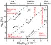 |
Fig. 1 Diagram indicating different regimes in the (n,G0) parameter space. The labelled points correspond to our reference models used throughout the paper (see Table 2). |
In this paper, we consider higher H column densities than included in Paper I, expanding coverage from columns corresponding to AV = 10 mag to columns corresponding to AV = 30 mag. The main constraint on this depth is the limit in the interpolation tables used in the PDR code for computing the self-shielding of CO. In general, the properties deep inside the molecular cloud (AV> 10 mag) are constant. This fact can be exploited to approximate the cloud properties at even higher AV values.
We note that all figures shown in main text of this paper correspond to PDRs of solar metallicity. We have, in fact, also considered other metallicities, including those as low as Z = 0.1 Z⊙ which characterize the most metal-poor dwarf galaxies as well as Z = 2 Z⊙ typical to galaxy centres. At any fixed AV, the corresponding H column density (NH = N(H) + 2N(H2)) is taken to depend inversely on the cloud metallicity in a linear fashion. We illustrate this as follows. PDRs with the lowest metallicity and highest AV = 30 mag considered will have NH = 5.6 × 1023 cm-2 compared to NH = 9.4 × 1021 cm-2 for clouds with a Z = 2 Z⊙ and an AV = 10 mag. Figures corresponding to non-solar metallicity conditions can be found in the Appendix.
2.1. Mechanical heating
A major conclusion of Paper I was that mechanical heating must not be neglected in calculating heating-cooling balances. Addition of a modest amount of mechanical heating to the cloud volume, corresponding to no more than a small fraction of the UV surface heating, already suffices to alter the chemistry of the PDR significantly.
The PDR model grids in Paper I were parametrized by n (first axis – horizontal axis), G0 (second axis – vertical axis) and Γmech (per unit volume, third axis). The parameter space was sampled by picking equidistant points in log space for each axis. The dis-advantage of such a representation is that for all the models each grid (as a function of n and G0) has the same amount of Γmech independent of n. For example, a cloud with n = 1 cm-3 would have the same amount of Γmech added as one with n = 106 cm-3. What might be a huge amount for the former cloud would be negligible for the latter. It is thus preferable to parametrize Γmech adaptively for each density level. In the following, the third axis is replaced by the new parametrization of Γmech. This new parametrization is defined using the symbol α where: 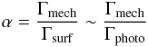 (1)where Γsurf is the total heating rate at the surface of the PDR (at AV = 0 mag), and Γphoto is the photo-electric heating rate. The expression relating it to n and G0 is Γphoto = ϵ0G0n, where ϵ is the heating efficiency. The treatment of mechanical heating in terms of the total surface heating is to a high degree of accuracy equivalent to a parametrization as a function of Γphoto. Γphoto is linearly proportional to n. For a certain section in α (in the third axis) each model thus has a Γmech proportional to its density. We note that this new parametrization is also equivalent to saying that Γmech is added per unit mass, since multiplying n by mH (the mass of a hydrogen atom) corresponds to a mass density.
To make this clear, we will now consider an example. The case α = 0 corresponds to a situation where no mechanical heating is present in the PDR (what we call this a reference or pure PDR model). On the other hand, the case α = 1 represents a model where the amount of mechanical heating added to the reference model, is equivalent to the heating at its surface. We now point the reader to the right panel of Fig. 2, which is a grid of reference models (i.e. a section in α = 0). For example, the surface heating for a model with n = 104 cm-3 and G0 = 103 is ~10-19 erg cm-3 s-1. In a grid with α = 0.01, this model would have an amount Γmech = 0.01 × 10-19 = 10-21 erg cm-3 s-1 added to its heating budget. More such examples are summarized in Table 1.
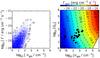 |
Fig. 2 Left: mechanical heating rates applied to the softened particle hydrodynamics (SPH) simulation of a dwarf galaxy (Pelupessy 2005; Pelupessy & Papadopoulos 2009). The maximum heating rate is ~10-22 erg cm-3 s-1. Right: surface heating (Γsurf) for zero mechanical heating (α = 0) for Z = Z⊙. The heating rates range from ~10-22 to ~10-20 erg cm-3 s-1 at n ~ 103 cm-3. An SPH particle with n ~ 103 cm-3 and a maximum Γmech (in the simulation) would have an α = 1 and 0.1 if its G0 is 1 and 103 respectively. The black points in the right panel correspond to the boundary points in n and Γmech distribution (plotted as open circles in the left panel). |
Mechanical heating rates for different densities and FUV luminosities for models whose metallicity is Z = Z⊙.
A simple recipe (also adopted in Paper I) for estimates of Γmech in a starburst is presented in Loenen et al. (2008). One of the main assumptions concerns the fraction of the energy of a supernova (SN) event transferred into heating the ISM (ηtrans), which was assumed to be 10%. However, ηtrans is not well known in general. The amount of turbulent energy transferred into heating the ISM, (Γmech), is also related to ηtrans. For this reason we consider values of α ranging for 0 to 1. This range would cover most heating rates that would be a result from the full range of ηtrans. As an example, α could be related to the local star-formation rate (SFR) in a starburst. In general, a higher SFR, would result in a high SN rate, thus a larger α as shown in Table 1.
Moreover, we used the mechanical luminosity curves in Leitherer et al. (1999) as an independent method of estimating the amount of Γmech that can be disposed into the ISM. In Leitherer et al. (1999) stellar population synthesis models are used to predict spectrophotometric properties of active star-forming regions. Figures 111 to 114 in that paper, provide predictions for the mechanical luminosity over a timespan of 1 Gyr, both for an instantaneous starburst (Lmech = 1040−1041 erg/s) and a continuous one (Lmech = 1042 erg/s). The mass of the stars formed during these two scenarios is 106M⊙. If we assume that this occurs in a box whose size is 100 pc (the same spatial scale used in Loenen et al. 2008), we obtain a Γmech ~ 10-20 erg cm-3 s-1 and Γmech ~ 10-22–10-21 erg cm-3 s-1 for the continuous and the instantaneous starburst scenarios respectively. In computing those estimates, we assumed that the mechanical luminosity is fully absorbed by the ISM since they occur over a timespan of at least 50 Myr, which is much longer than the chemical timescale.
Our final attempt to estimate Γmech relied on extracting the mechanical feedback from softened particle hydrodynamics (SPH) simulations of dwarf galaxies (Pelupessy & Papadopoulos 2009). There the mechanical heating is computed self-consistently in the SPH code. In the left panel of Fig. 2, we show the mechanical heating rate (per unit volume) as a function of the gas density of the SPH particles. It is quite comforting to note that, although the previous two methods were quite simplistic, the estimated mechanical heating rates are close to those obtained by the SPH simulation for the same density range.
2.2. Radiative transfer
Two methods were used in computing the radiative transfer of the atomic and molecular lines. Those of the atomic fine-structure (FS) lines were computed self-consistently within the PDR code (see Meijerink & Spaans 2005, for the details). For these lines the temperature gradient within the slab has been taken into account.
In computing the emission of the molecular species the statistical equilibrium non-LTE radiative transfer code RADEX (Schöier et al. 2005) was used. In order to account for clouds with different depths, the various emission were computed for different AV. This is equivalent to saying that we considered a semi-finite slab illuminated by a UV source from one side (the primary UV source). In using this approximation the UV flux from a source which could be on the other side of the truncated slab model, is ignored. Accounting for that second source would be important in the case when AV is low (<1 mag) and when the lines are optically thin. Although the lowest AV we considered was 5 mag, the worst case scenario even for high Av is when the secondary UV source (from the other side) has the same strength as the primary. In this case, ignoring the secondary UV source would reduce the emission by at least half the amount. For our purposes, since we would be looking at line ratios and at clouds with AV> 5 mag, we expect this approximation to be satisfactory for our purposes. Hence, for simplicity we assume that the semi-infinite slab is illuminated by a UV source from one side only. There are PDR codes which allow for a secondary UV source, for example Le Petit et al. (2006). An even more advanced PDR code which allows for an arbitrary 3D geometry has been developed by Bisbas et al. (2012).
The LVG approximation upon which RADEX is based does not take into account a PDR temperature gradient. For the molecular species, this is not crucial, for two reasons: firstly, molecules are only abundant in regions beyond AV ≳ 5 mag. In those regions the molecular abundances are at least two orders of magnitude higher than those close to the surface of the PDR (AV = 0 mag). Secondly, deep into the cloud where AV ≳ 5 mag temperatures are practically constant, very different from the steep temperature gradients close to the PDR surface.
Although the temperature is almost constant in the molecular zone, we tried to account for the contribution of the temperature gradient of the atomic and radical zones by using a weighted average of the quantities required to compute the emission. The gas kinetic temperature and the densities of the colliding species (mainly H2) were weighted against the density of the species of interest. The weighted temperatures are ~3% higher than the saturated kinetic temperatures in the molecular zone. This is due to higher kinetic temperatures at the surface compared to those in the molecular zone. In contrast the weighted density of the colliding species was about 5% lower than those in the molecular zone. This reflects the fact that H2 has a much lower abundance near the surface of the cloud compared to that at the molecular zone. These two counteracting effects, higher temperature and lower abundances result in a 1% increase in the emission compared to the case where no weighting was done.
The densities of the colliders are also weighted with respect to the abundances of species whose emission are being computed. The colliders considered were H2, H+, He and e−. Finally, a background radiation field corresponding to that of the current day cosmic microwave background (CMB) is used by RADEX. One of the assumptions we adopted, which cloud effect the outcome of the line ratios of 13CO to CO, is the elemental abundance of C and 13C. Since we opted to keep the number of parameter low for this exploratory investigation, we chose C/13C = 40 for all our models, even for models with higher and lower metallicities. The actual ratio could be as high as 90 and as low as 20 in our galaxy (Savage et al. 2002). Since we picked a lower value, we expect that variations over the possible range would only decrease the emission of 13CO; hence leading for line ratios involving 13CO/CO to decrease.
One of the main advantages offered by the use of RADEX (one-zone approximation) over a calculation based on the temperature gradient is the much greater speed of computation. For each model, the LVG approximation requires only one computation of the population densities. In contrast, it would have been necessary to compute the population densities for each slab of the discretized PDR when taking the temperature gradient into account.
It still remains to decide what micro-turbulence line width to use. Since most molecular line emission emanates from the shielded region where AV> 5 mag and where the gas is relatively cold, the line widths there are expected to be low. Again, here we resort to the simulations of Pelupessy & Papadopoulos (2009), where for such clouds, the velocity dispersion is of the order of few km s-1. Hence, for simplicity we used a micro-turbulence line-width of 1 km s-1 for all our models. We considered other line widths as well but the effect on the line ratios was negligible. We note that this line width should not be confused with the measured (observed) line-width. The measured line-width would be due to the contribution of multiple clouds along the line of sight. For extra-galactic sources, this line-width would be much larger than the micro-turbulence line-width.
As a check on the validity of using LVG models, we compared the emission grids computed with the LVG approximation to those computed by Meijerink et al. (2007). Although the grids in Meijerink et al. (2007) have been computed taking into account the temperature gradient in the PDR, they agree quite well with the ones we computed here with RADEX. As an independent check, the grids without Γmech agreed quite well with the ones computed by Kaufman et al. (1999).
3. Results
Atomic fine-structure and molecular emission lines are studied in order to see how mechanical feedback could affect their emission and their various line ratios. Here we present results from the reference models summarized in Table 2, and highlight some emission grids. The grids for different column densities are presented in the Appendix. We start by presenting results of the atomic lines, followed by those for molecular species. For each of the species considered we highlight the main chemical and radiative factors which effect their emission. Once we have characterized the effect of mechanical feedback on the emission of the reference models and the model grids, we proceed by highlighting trends in the line ratios which could be used as diagnostics for mechanical feedback in the ISM.
Reference models for typical PDRs used in this paper.
3.1. Atomic species – intensities
FS lines such as [OI] 63 μm and [CII] 158 μm are the dominant coolants in PDRs. High temperatures (>100 K) are necessary to have a bright emission of those lines. Thus most of the emission originates from the surface layer of the PDR where NH< 1021 cm-2. The temperatures drop with increasing NH as such column densities are optically thick for FUV photons (Hollenbach & Gorti 2009). In Fig. 3 we show the integrated cooling rate as a function of depth (AV) for M1. From a qualitative point of view, the cooling budgets for the remaining models are similar. The purpose of this figure is to illustrate the steep dependence of the FS cooling as a function of AV. We also see here that the cooling due to the lowest transition of the molecular species considered adds up to less than ~1% of the total cooling. For simplicity, we do not include this small contribution in the thermal balance, albeit it is not quite negligible.
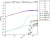 |
Fig. 3 Integrated cooling rates (in erg cm-2 s-1) |

Although most of the FS emission emanates from the PDR’s surface section, the molecular zone also contributes. This contribution of the molecular zone to the FS cooling is important when considering line ratios. It depends on the location of the C+/C/CO transition zone. A fast transition (as a function of AV) from C+ to C, would result in a lower abundance of C+ (thus lower emission). Usually, the AV where the C+/C/CO transition zone occurs is closer to the surface for PDRs with high densities than clouds with low densities. This phenomenon is described in more detail in Kazandjian et al. (2012). For example, in low-density PDRs the abundances of C+ (xC+) decreases slightly from ~10-4 (at the surface) to ~10-5 in the molecular zone. However, a much greater decrease in xC+ is observed in the molecular zone of medium and high-density PDRs; there xC+ decreases to ~10-10. Consequently, we expect to find higher contributions to C+ cooling from the molecular zones in low- density clouds than in high-density clouds.
A similar analysis applies to the other FS lines of C and O. For example in clouds which are highly dominated by UV radiation (see Fig. 1) atomic abundances remain relatively high in the molecular zone. At the surface 10-6<xC+< 10-4 and xC ~ 10-4 due to the high flux of FUV photons which can penetrate deep into the clouds. Hence recombination is less effective in locking the atoms into molecules. At densities n> 103 cm-3, the FUV photons are blocked by higher columns of CO resulting in xC+< 10-8 and xC< 10-6.
The intensity of the emission depends mainly on the chemical abundances of the species in question (discussed in the previous two paragraphs) and strongly on the kinetic temperature of the gas. Here we investigate the effect of Γmech on the emission, from the atomic and molecular zones, by looking at its effect on the kinetic temperature of the gas. In general we expect the emission to be enhanced as Γmech is introduced into a PDR. At the surface, mechanical feedback increases the temperatures at most by a factor of three, even for the highest Γmech considered. As an example, in the low G0/n (~0.01–10) models such as MA1 and MA2, the surface temperature increases from 110 K to 300 K without mechanical heating (α = 0, see Eq. (1) and Fig. 2) and from 2200 K to 4500 K for maximum Γmech (α = 1.0), respectively. Note that the surface of low density PDRs is a lot more sensitive to Γmech compared to the high density ones. Moreover, the temperature increase in the molecular zone is much greater. For instance in the low density PDRs, we see a boost from ~10 K to 100 K in MA2 and MA1 whenever Γmech = 0.1Γsurf.
Critical densities and the transition (excitation) energies for the atomic FS lines and the molecular lines.
We now turn our attention to the contribution of the molecular zone to the integrated luminosity of the FS lines. In pure PDRs (α = 0) which are in the G0/n ≫ 1 regime, at least 2% of the integrated luminosity comes from depths with AV> 5 mag. Since Γmech increases temperatures in the molecular zone, we expect the FS line emission to increase as well (this is explained in more detail in Sect. 3.3). For instance, when α = 0.25 the contribution of the molecular zone increases to ~10% for clouds with AV = 10 mag. For clouds with higher AV (~30 mag) this contribution increases further up to 50%.
In the top panel of Fig. 4, we show the emission grid of the [CII] 158 μm FS line. This grid agrees very well with that shown in Fig. 3 in Kaufman et al. (1999). In the lower panel, we illustrate the relative changes in the emission of that same grid as a function of α. We see that the [CII] 158 μm FS line emission depends weakly on Γmech whenever it is below 0.5 Γsurf (α< 0.5). Whenever α ≥ 0.5 low density PDRs such as MA1 and MA2 show an increase in the emission by up to a factor of two. The mid- and high-density PDRs whose G0> 102 are hardly effected. The emission of [OI] 63 μm, [CI] 369 μm, and [CI] 609 μm exhibit a stronger dependence on Γmech. These grids are shown in Fig. A.1.
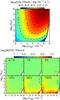 |
Fig. 4 Top: reference grid for the [CII] 158 μm line emission for PDRs without mechanical heating. Bottom: [CII] 158 μm line emission corresponding to different value of α labelled at the top of each panel. Each model in the grid has an additional amount of heating introduced to its energy budget. The added Γmech is in terms of a percentage of the surface heating (as explained in the methods section). Each grid shows the percentage change (increase or decrease) in emission relative to that in the reference grid in the top panel. For instance, when Γmech = 0.5 Γsurf (α = 0.5) (panel with the 50% label), the emission in MA1 is enhanced by a factor of ~3. A decrease in emission is observed only when Γmech> 0.5Γsurf to the right of the contour line at M4. We define the relative change as R = I(α) /I(α = 0), where I(α) is the emission intensity of the line at a specific value of α. Here and in all such subsequent plots the dashed contour line traces R = 1. On this line the emission with and without extra heating are the same. In other words, models on this line experience no change in the emission because of Γmech. In general “redder” regions correspond to enhanced emission, whereas “bluer” regions indicated regions where emission are suppressed. |
As a basis for discussion, we first highlight some of the main features of the FS emission grids in the absence of any Γmech contribution. (1) Emission intensities increase as G0 increases (see the top panels of Figs. 4 and A.1). This is caused by the ability of the FUV photons to penetrate deeper into the cloud at fixed n but higher G0, thus leading to a thicker atomic region. (2) Emission peaks near the critical densities of the lines (ncr hereafter). Those ncr are around 103 cm-3 with the exception of the critical density of the [OI] line which lies in the high density region. Both excitation energy Eul/kB and ncr for all the lines are listed in Table 3. (3) The emission intensities range from 10-6 erg cm-2 s-1 to 10-2 erg cm-2 s-1, spanning four orders of magnitude. This is significantly brighter than the molecular emission (see Sect. 3.3), which peaks at 10-5 erg cm-2 s-1. The range in the intensities of the atomic fine-structure lines is narrower than that of the molecular lines. (4) When Γmech is introduced the emission in enhanced for n<ncr; the opposite is observed for n>ncr. This is particularly valid for the neutral and atomic species (see the bottom panels of Figs. 4 and A.1).
Here we focus on the last point mentioned in the previous paragraph. Particularly we try to determine the reason causing the different behaviour of the emission for n<ncr vs. n>ncr. The boost in the emission could be due to an increase in temperature, or in abundance, or both. By analysing the chemistry we see that the dominant reactions remain the same (up to α ~ 0.1) for n<ncr. Moreover there are no fundamental changes in the abundances for n<ncr. This ties the emission boost to the increasing amounts of Γmech that raise the gas temperature, particularly in the molecular region.
Let us now consider the part of the parameter space in the grid where n>ncr. The emission tends to decrease whenever α> 0.1. The only exception to this occurs in the emission grid for the [OI] 63 μm line (see rightmost panel in the bottom row of Fig. A.1). At such densities, O maintains a much higher abundance than C+ in the molecular zone. Hence the strongest decrease is seen for the two neutral carbon lines [CI] 369 μm and [CI] 609 μm (see left and middle panels of Fig. A.1) whereas the opposite is observed for [OI] 63 μm. We will discuss each of those below.
The high density region of the [CII] 158 μm grid reveals a decrease in the emission only in extreme cases (α> 0.5). This is seen most clearly to the right of the dashed line in the panels for α = 0.1, 0.5 and 1 in Fig. 4). This is simply because C+ becomes un-abundant at high densities (n ≳ 105 cm-3).
The emission of [OI] 63 μm is more interesting but less trivial to explain, since it is the result of an interplay between the cooling due to the FS lines and the additional Γmech. We have already mentioned that [OI] 63 μm is the dominant cooling line in all the models. As Γmech is added more cooling is required to maintain a thermal balance. This occurs by increasing the gas temperature throughout the PDR which in turn boosts the total cooling rate by increasing the [OI] 63 μm emission. At the densities of interest here (n> 104 cm-3) and with α> 0.5, xO decreases from 10-4 to 10-8 in the molecular zone due to the dominant reaction of O with OH. Notwithstanding the steep decrease in xO, the [OI] 63 μm emission increases because of the much higher temperatures.
Finally, the reduction in the [CI] emission (at high densities) when Γmech is introduced, is due to xC decreasing by an order of magnitude in the atomic region of the PDR; dropping from ~10-4 to ~10-5 where most of the emission comes from. We discuss this for an extreme PDR with conditions typical for an extreme starburst (n = 106 cm-3 and G0 = 106). There the emission decrease is greatest. This decrease is due to the reduced production rate (by one order of magnitude) of C through the neutral-neutral reaction of H with CH. Moreover, higher abundances of H2 in the atomic region enhance the radiative association reaction of C with H2, leading to a faster destruction of C. These two processes results in a reduction of xC throughout the PDR leading to lower emission.
The different dependence on Γmech throughout the grids of the lines encourage us to look in detail at the various combinations of line ratios in an attempt to identify effective diagnostics for Γmech. We first summaries the most important model emission features that play a role in determining the ratios:
-
For pure PDRs (without Γmech) we can safely say that the majority of theFS emission are from the surface of the cloud and up toAV = 10 mag. Particularly, [OI] 63 μm and[CII] 158 μm saturate atAV ~ 5 mag.
-
When Γmech is introduced, the molecular zone contributes increasingly to the integrated emission of the lines, especially those of [CI]. When n<ncr more than half of the emission in these lines is from the molecular zone. Hence, line ratios might depend on the column densities of the PDRs considered.
-
As Γmech increases, emission of the FS lines for clouds with n<ncr increases; whereas it tends to decrease above that density (except for [OI]).
3.2. Atomic species – line ratios
So far we have touched upon the intensities of the emission of FS lines. What actually matters is the relative enhancement of one emission line compared to another (i.e. the line ratio); this is a commonly used technique since understanding line ratios sheds insight on the underlying excitation mechanism(s) of such emission. In Fig. 5 we show (for the reference models) all the possible combinations of line-ratios of the FS lines that we considered. The analogous figures for metallicities either higher or lower than solar are presented in Fig. A.2. We note that the line ratios apply to fixed cloud sizes (AV = 10 mag).
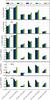 |
Fig. 5 Fine-structure line ratios for different values of Γmech (Z = Z⊙) for the reference models. |
The very low-density models (MA1 and MA2) show a distinctive response to Γmech in comparison to the rest of the models. Only in these two models, some of the line ratios (expressed on log-scales) change sign i.e. the ratio changes from being below unity to above unity or vice versa due to one line becoming brighter than the other.
For instance, in MA1, the ionized to neutral atomic carbon line ratio [CII] 158 μm/[CI] 369 μm shows a very nice dependence on Γmech. It decreases from ~15 to unity as Γmech increases. A similar behaviour is observed for MA2, but the ratio saturates to ~3 at high α. Another interesting line ratio is that of neutral oxygen to neutral carbon ([OI] 63 μm/[CI] 369 μm), which exhibits a very strong response to Γmech. The ratio decreases as α increases. The reason for this is that the [CI] 369 μm line is enhanced (and becomes stronger than the [OI] 63 μm line) due to the low energy of the [CI] 369 μm transition (24 K) compared to the 228 K of the [OI] 63 μm line. Hence, the [OI] 63 μm emission remains restricted to the surface, whereas the total emission of [CI] 369 μm gets a significant contribution from the deeper molecular interior. This line ratio decreases by approximately a factor of ten for MA1 (from ~20 to ~3) when Γmech is as low as 5% of the surface heating. A less distinctive behaviour is observed in MA2, where the line ratio decreases from ~2 to ~1 and increases again to above 2 for α = 0.5. In MA1, the ratio of the principal cooling lines, neutral oxygen to singly ionized carbon ([OI] 63 μm/[CII] 158 μm), has a weak dependence on Γmech. It increases only for extreme mechanical heating rates corresponding to α = 0.5. More interestingly, in MA2 the ratio has a stronger dependence of Γmech approaching unity (from ~0.3) as α increases. This is explained by the fact that as α increases, temperatures increase as well. Since xO is about 100 times higher in the molecular zone than xC, the [OI] 63 μm emission increases. This occurs despite the fact that the transition energy for the [CII] 158 μm line is less than half that of the [OI] 63 μm line. A similar behaviour is observed in M1, but there the ratios increase from 1 to ~3.
The neutral carbon-carbon line ratio [CI] 369 μm/[CI] 609 μm is particularly interesting since it involves FS lines of the same atomic species; hence the line ratio depends purely on the radiative properties of the lines and neither on the chemistry nor the column density. In MA1, we see a steady increase in the ratio from 1 to ~5 for α = 0.05. This can be easily explained. As Γmech causes temperatures to rise, the upper levels become more populated, so that the third level involving the [CI] 369 μm line becomes brighter than [CI] 609 μm. For a detailed discussion on level populations see Sect. 3.3.
The C[II] 158 μm/[CI] 609 μm and [OI] 63 μm/[CI] 609 μm ratios do not exhibit any very interesting dependence on Γmech. They are shown just for completeness.
The high-density models M1 to M4 exhibit a slow monotonous (either increasing or decreasing) dependence on Γmech. The ratios in these models are generally ≳10 even for α = 0. This is also true for extreme mechanical heating rates α = 1 (except for [OI] 63 μm/[CII] 158 μm in M1). Unlike the low density models, models M1 to M4 exhibit a jump in the line ratios only when α ≳ 0.5.
In summary, what we have found in this section that [CII] 158 μm/[CI] 369 μm, [OI] 63 μm/[CI] 369 μm and [CI] 369 μm/[CI] 609 μm are good diagnostic line ratios for low density clouds. One can use those lines to constrain Γmech if the density, G0 and the AV of the object are known. Those line ratios show a stronger dependence on Γmech at higher or lower metallicities as well, except in models at Z = 0.1 Z⊙ (see Fig. A.2). However, further investigation is needed in-order to see if atomic line ratios are good diagnostics of mechanical feedback for the whole range in density, G0 and AV.
In addition to the reference models, the grids of the line ratios from which those models were picked are presented in Fig. A.3.
3.3. Molecular species
The molecular emission lines were computed with LVG models, unlike those of the atomic species which were computed within the discretized PDR. We utilized the LVG code RADEX (Schöier et al. 2005) in computing all the emission intensity grids. In this paper, we have limited ourselves to the rotational line emission from CO, 13CO, HCO+, HCN, HNC, CS, and CN.
We first present an analysis that is common to most of the molecular lines considered. In pure PDRs (α = 0), the gas temperatures in the molecular region are very low (10 ~ 15 K) and vary little within the grid (see the grids corresponding to α = 0 in Appendix B for all the molecular species). Thus whenever the gas density of a cloud is below the critical density (ncr) of the line considered, the chemistry determines the shape of the contours in the emission grid. There the contour lines are independent of G0 and appear as almost vertical lines. Also in the absence of Γmech, the emission contours follow the shape of the temperature contours of the molecular region. This is particularly valid in the case of the high-J transitions. However, when we introduce Γmech, the chemistry is altered significantly along with the gas temperature. This causes the emission to increase by orders of magnitude (cf. the figures for CO with Γmech in the Appendix).
On the other hand, for densities above ncr, the contours in the emission grids depend mainly on temperature. This is not surprising, as we may demonstrate by considering a simple two level system. The ratio of the upper population density (x2) to the lower one (x1) at equilibrium is (Draine 2010): 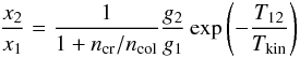 (2)where ncol is the density of the colliding species (mainly H2). g1 and g2 are the degeneracies of the lower and upper levels respectively and T12 is the energy difference of the two levels in Kelvins (E12/kb). For simplicity, we assume ncol = n(H2), and also ignore a second term on the right involving the radiation temperature (Trad) that introduces only minor changes in the LVG treatment (since Trad = Tcmb ≪ Tkin in general).
When ncol ≫ ncr, this equation reduces to: 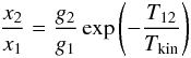 (3)which is independent of the gas density, and depends only on the kinetic gas temperature. Also, when ncol>ncr, all the lines are thermalized, and the excitation temperature is effectively equal to the gas temperature. Although these equations are for a two-level system, they provide a general idea of what might be happening in a multi-level systems (which might include multiple colliding species whenever the rates are available).
As Γmech is introduced, the higher transitions gain prominence since relative temperature increases are high. This in turn leads to increased high-level populations (see the left panel of Fig. 6). Another way to look at the pumping of the higher levels is by looking at the collision rate coefficients K12 and K21. Ignoring degeneracies, those two are related via K12 ~ K21exp(−T12/Tkin).
Another interesting common feature is the optical depth at the line centre, τ0. We observe that it decreases as a function of increasing Γmech. As temperatures increase, more levels get populated leading to smaller optical depths. These are shown in Fig. 6, which shows the CO ladder along with curves for τ0 for a range in Γmech. In the right panel, the trend in τ0 is clearly visible.
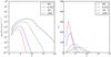 |
Fig. 6 CO ladders for a PDR model with n = 103 cm-3 and G0 = 103 for different values of mechanical heating. The numbers in the legend correspond to Γmech in terms of the surface heating. Left: CO line intensities as a function of the rotational level J. Notice the boost in the intensities is much larger at high-J compared to low-J. Right: optical depth at the line centres (τ0) for the same lines. The optical depth generally decreases as a function of increasing Γmech, but the most significant effect is that the low-J CO lines become optically thinner with τ0 ~ 1. |
CO and 13CO CO is the second most abundance molecule in the ISM after H2. Since the critical density of the CO(1–0) rotational line is moderate (see Table 3), it is a good tracer of molecular gas with average densities. The critical densities increase gradually as we go higher up the CO ladder, reaching ~106.5 cm-3 for the 16–15 transition2. In Fig. 7 we show the grids for CO J = 1–0 emission. In Fig. 8, we show the relative increase/decrease in CO J = 1–0 emission as a function of Γmech. The analogous grids for the CO J = 2–1, 3–2, 4–3, 6–5, 7–6, 10–9 and 16–15 transitions are presented in Fig. B.1 (and a subset of those for the 13CO lines) are displayed in Fig. B.2. We note that we will be using 12CO and CO interchangeably in referring to carbon monoxide.
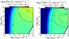 |
Fig. 7 Emission intensity grids of CO(J = 1–0) and 13CO(J = 1–0) transitions for the 1D-PDR models. The emission of the models in the grid correspond to an AV = 10 mag, which amounts to a column density of H, NH ~ 1022 cm-2 at solar metallicity. The intensities were computed using the RADEX LVG code. A line-width of 1 km s-1 was used. No mechanical heating is added for the models in this grid. This is used as a reference grid for the ones in which Γmech is introduced (see Fig. 8). |
 |
Fig. 8 Relative change in the emission of the CO J = 1–0 rotational line for different values of Γmech. The colours in the panels correspond to the relative change of the emission with respect to the reference grid in the left panel of Fig. 7. See also the caption of Fig. 4. |
At low densities (n< 10 cm-3), the emission of CO is very weak (~10-10 erg cm-2 s-1) compared to emission at mid- to high densities (n> 103 cm-3). This is obvious in Fig. B.2. As was mentioned also earlier, we notice that at such low densities the emission contours show almost no dependence on G0. This is simply explained by the fact that there are few collisions to excite the upper rotational levels, and that the background dust emission (which is only weakly dependent on G0) is dominating. Another contributing factor is the low gas temperature (~10 K) in the molecular zone. On the other hand at mid- and high-densities, where n ≳ ncr of CO(J = 1–0), we start seeing a strong dependence of these emission on G0.
In general the emission intensity is positively correlated with Γmech, i.e. it increases with increasing Γmech (see Figs. 8, B.1, B.2). The only exception occurs at some of the high density regions in the CO(1–0) and 13CO grids. We can see such a behaviour in the upper right corner of the CO grids when α = 0.5 and 1. In the 13CO grids the emission decrease is clearest (and covers a larger part of the grid), for example see the J = 1–0, J = 2–1 and J = 3–2 grids in Fig. B.2.
In well-irradiated, low-density regions (n<ncr and G0> 10), the emission increases up to two orders of magnitude (see red regions in Fig. 8). This is caused by (1) a rise in the temperature induced by Γmech; and (2) a higher abundance of CO (and 13CO), causing a double increase. The abundance of CO is boosted because its is accelerated via the reaction H + CO+ → CO + H+.
At the higher densities (n>ncr and ≫ ncr) the response to Γmech becomes weaker. More than one factor contributes to this. From the thermal perspective the temperatures in the molecular regions are already high (~50 to 100 K). This is due to the tight coupling between dust and gas. Hence the relative increase in the gas temperature is small, in contrast to what happens in the low-density models. Another contributing factor is the decrease in the abundance of CO. In the absence of Γmech, most C atoms are locked in CO molecules. For extreme Γmech (α ≥ 0.5) the abundance of most molecules, including H2, decreases drastically (Kazandjian et al. 2012); leading to xCO lower by almost 3 orders of magnitude (from ~10-4 to ~10-7).
Although we would suspect that the higher temperatures (due to Γmech) would lead to enhanced emission, the reduced abundance and column density of CO counteracts that enhancement. These two effects combined lead to a small relative increase in emission. As an example, for low densities an increase in the emission by one order of magnitude is easily attained for α = 0.01. On the other hand an α = 0.1 is required to enhance the CO emission by the same factor in the high density region of the grids (cf. bottom-left panel of Fig. 8). The only exception where a decrease in the emission is observed occurs in the CO(1–0) line. This is not surprising, since in looking at the left panel of Fig. 6 we see that the 1–0 transition is weakly effected by Γmech (compared to the higher transitions). So a reduced N(CO) leads to lower emission of the 1–0 line.
A similar behaviour is observed for the 13CO emission which is, however, more sensitive to Γmech than 12CO. In particular, as Γmech increases, the mid- and high-density regions show a stronger decrease in the emission of the first three J transitions. This decrease is due to a reduced N(13CO) and an already low optical depth. N(13CO) is about five times lower than N(12CO). Moreover the Einstein A coefficients of 13CO are about 20% lower than those of 12CO. Hence the upper levels, which are mainly excited collisionally, are de-populated less frequently, and a higher upper-level population density is maintained. We see that these two factors lead to the reduced optical depth of 13CO. At mid- and high-densities N(13CO) decreases as α increases. Since the optical depth is already low, it neither plays a significant role in blocking the emission nor in enhancing the emission by allowing “trapped” radiation to escape from the cloud; this is also true when the cloud becomes more transparent as α increases. Consequently, since intensity is proportional to the column density of the emitting species, a decrease in N(13CO) results in lower emission. On the other hand, the J> 3−2 transitions show enhanced emission all over the grid. This occurs despite the reduced column densities of 13CO. High kinetic temperature due to Γmech enhances the strong pumping of the associated level populations; eventually, this counteracts the effect of the reduced N(13CO) on the emission.
Although the generic behaviour of the CO and 13CO grids are similar, the differences among them are interesting enough to take a closer look at their line ratios. Especially for ones involving the low-J lines where the 13CO lines are optically thin.
In Fig. 9, we show the line ratios for our reference models. These ratios include transitions for lines within the CO ladder (left panel), the 13CO ladder (middle panel), and the 13CO to 12CO line ratios (right panel). The ratios between high-J and low-J transitions show a strong dependence on Γmech. For example, in M3 the CO(16–15)/CO(1–0) ratio changes abruptly from ≲0.1 to >100 when α> 0.05. A similar behaviour is observed for the corresponding 13CO ratio. In Fig. 6, we see that the optical depth of J = 16–15 CO is almost unaffected as Γmech increases, whereas that of the J = 1–0 line decreases rapidly from ~100 to ~1. The opposite is observed when it comes to the intensity, where the J = 16–15 CO line emission increases by ~four orders of magnitude. This explains the huge increase in the ratio of those lines. This line ratio along with the ratio CO(16–15)/CO(10–9) are the only ones (among the ratios we looked at) that show a significant change for the high-density model M5 (see the top row of the middle panel in Fig. 9).
In medium- to high-density models, ratios involving low-J transitions are less sensitive to Γmech. Those ratios are almost constant in the high density models, since the lines are thermalized and the population densities do not change relative to each other. However in the low- and medium-density models MA1, MA2, and M1 the CO(4–3)/CO(1–0) ratio might be a good diagnostic for Γmech. In MA1 we see that this line ratio increases by a factor of ~10 (as well as the corresponding 13CO ratio). Because these are ratios within the same species, the increase is a pure measure of the radiative properties of the specie. As in the cases of MA1 and MA2, we are in the non-LTE phase. As the temperature increases, the upper levels are populated faster leading to stronger emission in e.g. the CO(4–3) line, which drives up the ratio.
The most interesting and useful behaviour of the 13CO/12CO (right panel of Fig. 9) occurs in the high density models M3 and M4. The ratios decrease monotonously from ~0.5 (for α = 0) to ~0.1 (for α = 1).
 |
Fig. 9 Line ratios of CO and 13CO for different amounts of Γmech (Z = Z⊙) for the reference models. |
We showed previously that the optical depth of CO decreases with increasing α. Also 13CO is optically thin in general. So for column densities corresponding to AV> 10 mag, we expect to have a steeper dependence of the line ratios of CO and 13CO on Γmech.
We summarize the main results of this section by emphasizing that in low density PDRs, the ratios of high-J to low-J emission lines of CO and 13CO might be useful diagnostics for Γmech. The line ratio of 13CO with its isotopologue CO are good diagnostics for Γmech in high-density PDRs. They show a strong and clear trend.
HCN and HNC HNC and HCN are linear molecules with very similar radiative properties in the infra-red regime. Both have (a) large dipole moments (3.05 and 2.98 respectively Botschwina et al. 1993). This allows both of them to be easily observed (b) both have high critical densities >105 cm-3 for the 1–0 transition (see Table 3). This renders them as good tracers for high-density molecular gas. In this paper, we consider the rotational transitions from J = 1–0 up to J = 4–3, which are commonly observed. Since the emission of these lines is very sensitive to temperature changes, they might be useful in identifying molecular clouds dominated by mechanical feedback. In Paper I we studied the column density ratios of the two species. We showed that HCN becomes more abundant than HNC as Γmech increases. Here we study the effect of Γmech on the emission of these two species and their ratios.
In the absence of any Γmech the emission grids show a very weak dependence on G0, as compared to their dependence on n. This dependence is illustrated in Fig. 10. This kind of dependence is generic to cases where the gas density is (much) lower than the critical density of the line considered; which is also the case here.
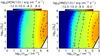 |
Fig. 10 HCN and HNC emission of the 1–0 line in the absence of Γmech (Z = Z⊙). |
In contrast to the weak dependence on G0, the dependence on Γmech is quite strong. The enhancements in the emission of HCN are stronger than those of HNC the bottom two rows of Fig. B.3). This is simply because HCN becomes more abundant than HNC. The main channel through which the conversion occurs is via the reaction H + HNC → H + HCN (see Meijerink et al. 2011, for a more elaborate discussion on the chemistry). This process becomes dominant for Tkin> 150 K in the molecular region (Schilke et al. 1992), which is achieved when α> 0.1. Below that threshold in α, HNC is equally destroyed via ion-neutral reactions with H3O+, especially at low densities. Another contributing factor to the increase in the abundance of HCN is its efficient formation via the neutral-neutral reactions with H2. For completeness’s sake, we note that the relative change in the emission of the J = 4−3 line is stronger than that of the 1–0 line for reasons discussed in Sect. 3.3.
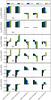 |
Fig. 11 Various line ratios of HNC and HCN as a function of Γmech (Z = Z⊙) for the reference models. |
In Fig. 11 we show the line ratios considered for HCN and HNC. Transition ratios such as HNC(4–3)/HNC(1–0) and HCN(4–3)/HCN(1–0) behave as expected (first two columns in the figure): with increasing α, they increase as well (since the higher levels are populated more easily at higher temperatures). In M1 and M2, the ratio increases quite fast linearly in log scale. Unfortunately, in M3 and M4 the ratios are almost constant and are thus of little use as a diagnostic for high-density PDRs.
Again in M1 and M2, the inter-species ratios HNC(1–0)/HCN(1–0), HNC(4–3)/HCN(4–3) and HNC(4–3)/HCN(1–0) are strongly dependent on Γmech. We see that for α = 0.5, the ratio HNC(1–0)/HCN(1–0) drops from ~2 to ~0.3. This is caused primarily by the difference in column densities caused by the chemical effects discussed above. Since those ratios depends monotonously on α (see M2 in Fig. 11), we may consider them as as a good diagnostic for such PDRs. This is not the case for M3 and M4. The line ratios have a weaker dependence on mechanical heating whenever α< 0.1. However an abrupt decrease (from ~0.3 to <0.01) is observed for α ≳ 0.5.
Interestingly enough at metallicities typical for galactic centre regions (Z = 2 Z⊙), clouds such as M4 show a significant dependence on α (see Fig. B.4). This is simply a result of the fact that a higher metallicity implies a higher column density of the gas and the species in question. In such situations, fluctuations of the abundances in the radical region play a minor role.
In summary, line ratios such as HNC(1–0)/HCN(1–0) and HNC(4–3)/HCN(4–3) are good diagnostics for Γmech in PDRs in the following cases: (a) at gas densities less than the critical densities of the lines mentioned; and (b) in high-density PDR environments such as galaxy centres with super-solar metallicities and starburst regions.
HCO+ HCO+ is another high density tracer. The critical densities (at 50 K) of its J = 1–0 and J = 4–3 emission lines are ~2 × 105 cm-3 and ~107 cm-3 respectively. The emission grids for both lines are shown in Figs. 12. The corresponding grids as a function of α are presented in Fig. B.5.
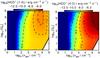 |
Fig. 12 HCO+J = 1–0 and J = 4–3 emission in the absence of Γmech for solar metallicity (Z = Z⊙). |
We will discuss only mid- and high-density models (n> 103 cm-3), since at lower densities the lines would be too weak to be observed. With increasing Γmech, the emission of the J = 1–0 line in the high density region (and G0> 105) decreases by a factor of ~2. At such high densities, xHCO+ drops by three orders of magnitude, leading to the reduced emission. We trace the source of the reduced abundance of xHCO+ to it slow production rate; which is reduced by an order of magnitude as α increases. This slowing down is mainly due to the reaction of the ionic species HOC+ and CO+ with H2 through which HCO+ is formed. The abundance of these two ionic reactants drops by factors of two and two hundred respectively as α increases, hence the slow production rate of HCO+. As long as the HCO+(J = 1–0) grid is concerned, the emission is enhanced everywhere else throughout the grid. See the dashed line in Fig. B.5.
For PDRs with moderate densities i.e. in the non-LTE phase of the rotational line of HCO+, the coupling between dust and gas is weak compared to that in high-density clouds. This weaker coupling results in a weaker dependence of the abundance on Γmech (since the physical conditions do not change much). However, the temperature does increase in the molecular zone where HCO+ is present. This increase in the temperature enhances the emission of the J = 1–0 line for densities n< 104 cm-3.
The J = 4–3 line responds in similar way to changes in Γmech, but the emission decrease only for α = 0.05 and 0.1. This emission is more sensitive to temperature changes because of the ease of populating upper levels. Thus the emission is boosted again for α> 0.1, despite the fact that xHCO+ decreases for n> 105 cm-3.
HCO+ is interesting because it behaves quite differently in the mid- and high-density regimes. It can be used as a diagnostic for both regimes in combination with other species (as we discuss below).
CN The critical densities of the CN(11/2–01/2) and CN(23/2–13/2) is in the high density part of the parameter space (see Table 3). Similar to HCO+, the emission grid of those lines also exhibits a peculiar dependence on increasing amounts of mechanical feedback. In looking at the abundance of CN, we see that at high densities xCN correlates negatively with α. The reduction in the abundance is caused by the high temperatures in the molecular zone of the PDR. The high temperatures leads to the destruction of CN, at a rate which is an order of magnitude higher compared to pure PDRs, through the reaction H2 + CN → HCN + C. The reduced abundance of CN results in the dimming emission as Γmech is introduced, which is evident in (Fig. B.6). Beyond α = 0.1N(CN) becomes too low, where the intensities (in both lines considered) decrease by a factor of 10.
On the other end of the parameter space (at mid- and low densities), N + CN → N2 + C is the dominant reaction for the full range in α. This reaction maintains a high xCN in that part of the parameter space, i.e. the region bounded by the dashed contour line in the bottom row (where α = 0.1,0.5,1.0) of the panel corresponding to CN in Fig. B.6.
CS This species has a very distinctive dependence on Γmech (compared to the other molecular species we have so far considered). In Fig. 13 we see that a region of suppressed emission sweeps across the grid from high- to low- density as α increases. This non-trivial behaviour is difficult to explain in detail.
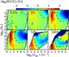 |
Fig. 13 Grids of the relative changes in the emission of the CS(1–0) line for different values of α (Z = Z⊙). See also Fig. 4 for a description of the colours. |
The ncr for CS is ~5 × 104 cm-3 and ~3 × 106 cm-3 for the J = 1–0 and J = 4−3 lines respectively (at 50 K). Up to α = 0.05 both grids indicate a strong decrease in the emission for n> 103 cm-3 and G0> 103. The reduction in the emission is as low as a factor of 50 for high density PDRs. As α increases further the emission of those PDRs starts to increase again relative to the case of α = 0. This increase reaches a factor of 50 for J = 4–3 transition. Meanwhile, the region where the emission are suppressed is pushed to lower densities and lower G0. This is a consequence of the chemistry. At the high densities, the drop in the emission is due to reactions with cosmic rays. Those reactions become dominant in destroying CS instead of the neutral-neutral reaction O + CS → S + CO; which otherwise is the dominant reaction in pure PDRs.
The strong dependence of the CS lines on α makes it a useful candidate for mechanical feedback.
 |
Fig. 14 Line ratios of HCO+, CN and CS for Z = 1 Z⊙ and AV = 10 mag for the reference models. |
In Fig. 14 we show the line ratio for CS, CN, and HCO+. In all the reference models the line ratio of HCO+(4–3)/HCO+(1–0) and particularly the interspecies CS/HCO+ ratios vary over more than one order of magnitude as a function of α. The CS(4–3)/CS(1–0) ratio shows some dependence on Γmech, but again those variations are small compared to the ones mentioned before. The line ratios CS(1–0)/HCO+(1–0) and CS(4–3)/HCO+(4–3) are more interesting. In looking at the CS grids in Fig. 13, we see that variations are well described in the CS/HCO+ ratios, which allows them to be used diagnostically to constrain Γmech in extreme starbursts. For instance a ratio less than 0.01 would imply an α ~ 0.05; whereas a ratio around 0.1 implies α> 0.1 (see last column in Fig. 14).
In M1 and M2, the line ratio behaviour is the same at higher or lower metallicities (see Fig. B.7). In M3 and M4, this ratio’s response to changes in α is slightly weaker at Z = 0.5 Z⊙. In the lowest metallicity case, CN(23/2–13/2)/CN(11/2–01/2) decreases to unity as α increases. This might be useful in probing Γmech in e.g. dwarf galaxies.
3.4. Other line ratios
Figure 15 shows some other molecular line ratios, selected to illustrate their importance as a diagnostic for Γmech in PDRs.
Most of the line ratios exhibit an order of magnitude change for α ≲ 0.25. Typical examples are HCO+(1–0)/CO(1–0) and HCN(1–0)/CO(1–0) in the high-density models such as M3 and M4. On the other hand, HCO+(1–0)/13CO(1–0) shows an irregular increase as a function of α in these models, but a strictly monotonous increase (from ~ 0.01 to 1) is observed in the lower density models M1 and M2.
Ratios involving lines of HCN with CO and HCO+ are excellent candidates for constraining Γmech. This is also the case at lower and higher metallicities (see Fig. B.8) for all the representative models. In some cases, such as HCN(4–3)/HCO+(4–3) in M4, the ratio increase from ~0.3 to 10 for α ~ 0.1. One drawback in the HCN(1–0)/CO(1–0) ratio is the degeneracy in its dependence on Γmech in M3. For example in the absence of Γmech, this ratio has a value of 0.3. It reaches a minimum of 0.01 (for α = 0.1) and increases back to ~0.3 for extreme cases where α = 0.5. Cases of such degeneracies can be resolved by simultaneously considering other line ratios, as we will demonstrate at the end of this section.
 |
Fig. 15 Line ratios with strong dependence on Γmech for Z = Z⊙ for the reference models. |
We draw special attention to the CN/HCN interspecies ratios. They have a very strong dependence on Γmech, showing a decrease by an order magnitude for the lowest transition ratios as α increases from 0 to 1.
In summary, we found that line ratios between CN, HCN and HCO+ are quite useful in constraining Γmech. This is true in particular for CN since Γmech seems to drive ratios to values well below unity for most clouds when α> 0.1. In high-density clouds whose heating budget is dominated by Γmech, line ratios of HNC/HCO+ tend to exceed unity.
4. Application
We have presented model predictions for line intensities and line ratios of many molecular species. However, we have not yet reflected on any observational data to which these models can be applied. In this section we use actual data and demonstrate a) the importance of molecular line ratios as a diagnostic for mechanical heating; and b) their usefulness as a tool for constraining it.
In Table 4, we present the range of line ratios involving HCN, HNC, CO and HCO+ for infra-red luminous galaxies taken from Table B.2 in Baan et al. (2008).
Observed ranges of molecular line ratios for some starburst galaxies.
We follow a simplistic approach to an ambitious goal. Our aim is to constrain (n, G0, AV, α) using the data at our disposal. The only major assumption we make is the metallicity of the source. Here we will assume solar metallicity.
In Fig. 16 we present a step-by-step procedure to constrain (n, G0, AV, α) using line ratio grids parametrized with those four quantities. Each small square represents a grid as a function of n (horizontal axis) and G0 (vertical axis), like all the previous grids that we have shown so far. Each collection of grids illustrates the constraining procedure for a certain AV. The collection of grids in Fig. 16 corresponds to AV = 5 mag. The ones for AV = 10 and 30 mag can be found in Figs. C.7 and C.8. In each column, grids for different α are presented.
In the top row of each collection, regions where the line ratio of HCN(1–0)/HNC(1–0) is within the observed range (see Table 4), are delineated in light blue. Clearly, the HCN(1–0)/HNC(1–0) ratio does not constrain all four parameters. However if AV and α are known, one can constrain the range in n and G0 for the source. For example, if we know a priori that AV = 5 mag and α = 0 (pure PDR), then the UV flux is constrained to G0> 105 (see the grid with α = 0 in the first row of Fig. 16) while the gas density is not constrained. On the other hand, if α is known to be 0.5 (which is quite extreme), then n and G0 are constrained to a much narrower region. Including the information about HCN(1–0)/HCO+(1–0) from Table 4, helps us better constrain all four parameters (see the second row in the mentioned figures). Although now n and G0 are better constrained (cyan regions), α is still degenerate. Similarly, HNC(1–0)/HCO+(1–0) fails in achieving our goal (yellow zones in the third row).
Based on our observation in the results section, that Γmech has a strong signature on high-J transitions (which was more or less ubiquitous for all species), we attempt adding ratios of observed lines involving a high-J and a low-J transition. We use the J = 4−3 transition of HCO+ of NGC 253 as a guide. It is clear that this ratio manages to constrain all four parameters, with moderate certainty to, AV ~ 5 mag, 103.5<n< 104, 104<G0< 104.5 and α ~ 0.1. This may not be a unique find; however, we expect the χ2 value (or the minimum for a proper statistical fit) to be close to the range constrained by this proof of concept simple demonstration.
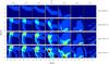 |
Fig. 16 Constraining the Γmech, AV, n and G0 for starburst galaxies. In this figure we illustrate the procedure used to constrain those parameters for AV = 5 mag, the figures for the remaining AV are in Figs. C.7 and C.8. Each row corresponds to a certain line ratio, and each column corresponds to a certain α. The colours correspond to regions where the observed line ratio in each grid is within the observed range of Table 4. In the first row regions where HCN(1–0)/HNC(1–0) is between 1.5 and 4.0 is shaded in light blue. In the second row we include HCN(1–0)/HCO+(1–0). The regions which are within the observed line ratios for both HCN(1–0)/HCO+(1–0) and HCN(1–0)/HNC(1–0) are shaded in cyan. In the third row, we introduce HNC(1–0)/HCO+(1–0), the region satisfying all three line ratios is shaded in green. We notice that green regions exist for all values of α in the third row. Hence we can not constrain α so far. It is only when HCO+(4-3)/CO(1–0) is included, α is constrained to 0.1 (red region in the α = 0.1 column) in the last row. Although much smaller red regions are also visible for α = 0.05 and α = 0.25, the global minimum would be most likely around α = 0.1 region. In applying a similar procedure to grids corresponding to AV = 10 and 30 mag, we do not observe any red region. |
5. Conclusion and discussion
We have studied the effect of Γmech on a wide range of parameter space in n and G0 covering six order of magnitude in both (1 <n< 106 cm-3 and 1 <G0< 106). Throughout this parameter space we investigated the most important and commonly observed molecular emission and atomic fine-structure lines and their ratios. The explored range in mechanical heating (Γmech) covers quiescent regions, with almost no star-formation, as well as violently turbulent starbursts. The SFRs for those range from 0.001 M⊙ yr-1 to ~100 M⊙ yr-1 respectively.
The two fundamental questions we try to answer in this paper are: (a) is it possible to constrain the mechanical heating rate in a star-forming region by using molecular line ratios as a diagnostic?; (b) how important is Γmech in recovering the molecular H2 mass of a star-forming region using observed molecular line emission such as those of CO?
Before discussing these questions, we state the main characteristics of mechanically heated PDRs we observed in our grids:
-
The most significant contribution of Γmech to the atomic fine-structure line intensities results from enhanced tem-peratures in the molecular zone. This is especiallythe case for the [CI] lines. For cloudswhose density is below the critical density of thoselines, half of the emission intensity emanates from themolecular zone. FS line ratios, such as[CII] 158 μm/[CI] 369 μm,[OI] 63 μm/[CI]369 μm and [CI] 369 μm/[CI]609 μm, are good diagnostics for Γmech inlow-density PDRs (n< 103 cm-3).
-
High-J to low-J transitional ratios of 12CO and 13CO, such as CO(16–15)/CO(1–0), are good diagnostics for Γmech over the whole density range considered. In contrast low-J CO line ratios, such as CO(2–1)/CO(1–0) or CO(4–3)/CO(1–0), are useful as diagnostics3 only for clouds with n< 103 cm-3.
-
The line ratios of 13CO/12CO (in both low-J and high-J transitions) have a strong dependence on Γmech. They decrease as Γmech increases. This complements the range in density where low-J transitions of 12CO (and 13CO) can be used as diagnostics for Γmech.
-
At high metallicities (Z = 2 Z⊙), HCN and HNC are very good diagnostics for Γmech when G0 ≳ 105, such sources include starbursts in galaxy centres.
-
Line ratios such as HCN(1–0)/CO(1–0), HCN(1–0)/HCO+(1–0), CN(11/2-01/2)/HCN(1–0), CN(23/2–13/2)/HCN(1–0), CS(1–0)/HCO+(1–0) show a strong dependance of Γmech, hence they are a good diagnostic of it.
The major conclusions of the paper, which we demonstrated in the application section is: low-J transitions alone are not good enough to constrain mechanical heating; ratios involving high-J to low-J transitions do a much better at that.
Another major conclusion is the importance of Γmech in constraining AV or, equivalently, the hydrogen column density NH, which can be used to determine the molecular mass of the cloud. In comparing Fig. 16 to the ones of higher AV in the Appendix, one can see that if Γmech is ignored, it is easy to under- or over-estimate the AV by a factor of five (or more). Ignoring Γmech also results in more than an order of magnitude error in estimating the n and G0. For instance in looking at the last row of Fig. 16, one can see that when Γmech is ignored, an error up to two orders of magnitude can be done in constraining the ranges of n and G0.
We emphasis that our approach in constraining the physical parameters of clouds using the observed line ratios, is just a proof of concept demonstration. Ultimately one must use more elaborate minimization methods to attempt to constrain the physical parameters. However, it is most likely that the parameters which best fit the observations, will be very close to the ones obtained using the method adopted in the application section. We leave it to the interested reader to make use of the grids which are published as well with this paper (see Figs. C.5, C.4, C.3).
We finalize our discussion by touching on the effect of cosmic rays (CR). Although it is outside the scope of this paper, we explored the effect of enhanced CR rates. Diagnostic line ratio grids for HCN, HNC and HCO+ are fundamentally different from those which are dominated by Γmech (see Fig. C.6). Hence, we expect that in using diagnostics presented in this paper, clouds which are embedded in environments where the CR rate is enhanced, would not be mistaken with clouds whose heating budget is dominated by Γmech.
Online material
Appendix A: Atomic species
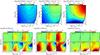 |
Fig. A.1 Fine-structure emission grids with and without Γmech (Z = Z⊙). Top: emission grids. Bottom: relative changes in the emissions as a function of α. The dashed contour traces the R = 1 line, where the emissions with and without extra heating are the same. (See caption of Fig. 4.) |
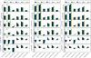 |
Fig. A.2 Line ratios for the reference models as a function of Γmech for the atomic fine structure lines, Z = 0.1, 0.5, and 2 Z⊙ in the left, middle and right panels respectively. |
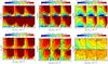 |
Fig. A.3 Atomic line ratio grids as a function of Γmech for AV = 10 mag (Z = Z⊙). |
Appendix B: Molecular species
 |
Fig. B.1 Top: emission grids of PDR models without mechanical heating for a selection of CO transitions for AV = 10 mag (Z = Z⊙). Bottom: relative changes in the emission as a function of α. The dashed contour traces the R = 1 line, where the emission with and without extra heating are the same. (See caption of Fig. 4.) |
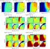 |
Fig. B.2 Top: emission grids of PDR models without mechanical heating for a selection of 13CO transitions for AV = 10 mag (Z = Z⊙). Bottom: relative changes in the emission as a function of α. The dashed contour traces the R = 1 line, where the emission with and without extra heating are the same. (See caption of Fig. 4.) |
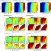 |
Fig. B.3 Top: emission grids of PDR models without mechanical heating for a selection of HCN and HNC transitions for AV = 10 mag (Z = Z⊙). Bottom: relative changes in the emission as a function of α. The dashed contour traces the R = 1 line, where the emission with and without extra heating are the same. (See caption of Fig. 4.) |
 |
Fig. B.4 Various line ratios of HNC and HCN for the reference models (see Table 2) as a function of Γmech for Z = 0.1 Z⊙ (left), 0.5 Z⊙ (middle) and 2.0 Z⊙ (right.) |
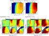 |
Fig. B.5 Top: emission grids of PDR models without mechanical heating for a selection of HCO+ transitions for AV = 10 mag (Z = Z⊙). Bottom: relative changes in the emission as a function of α. The dashed contour traces the R = 1 line, where the emission with and without extra heating are the same. (See caption of Fig. 4.) |
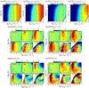 |
Fig. B.6 Top: emission grids of PDR models without mechanical heating for a selection of CN and CS transitions for AV = 10 mag (Z = Z⊙). Bottom: relative changes in the emission as a function of α. The dashed contour traces the R = 1 line, where the emission with and without extra heating are the same. (See caption of Fig. 4.) |
 |
Fig. B.7 Various line ratios of HCO+, CS and CN for the reference models (see Table 2) as a function of Γmech for Z = 0.1 Z⊙ (left), 0.5 Z⊙ (middle) and 2.0 Z⊙ (right.) |
 |
Fig. B.8 Various line ratios (at AV = 10 mag) of HCN, HNC, HCO+, CN, and CS which show a strong dependence on Γmech for the reference models (see Table 2) for different metallicities, Z = 0.1 Z⊙ (left), 0.5 Z⊙ (middle) and 2.0 Z⊙ (right.) |
Appendix C: Several model grids
 |
Fig. C.1 Grids of CO and 13CO line ratios for different values of α for AV = 10 mag. |
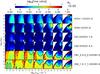 |
Fig. C.2 Grids of various combination of molecular line ratios for different values of α and AV = 10 mag. |
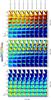 |
Fig. C.3 Grids of HCN and HNC line ratios for different values of α and AV. |
 |
Fig. C.4 Grids of HNC and HCO+ line ratios for different values of α and AV. |
 |
Fig. C.5 Grids of HCN and HCO+ line ratios for different values of α and AV. |
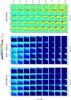 |
Fig. C.6 Grids of HCN, HNC and HCO+ line ratios (J = 1–0 and 8–7) for different cosmic ray ionization rates with AV = 10 mag. |
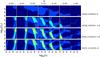 |
Fig. C.7 Constraining the Γmech, AV, n and G0 for starburst galaxies. Illustration for Av = 10 mag. See caption of Fig. 16 for details. |
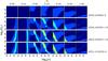 |
Fig. C.8 Constraining the Γmech, AV, n and G0 for starburst galaxies. Illustration for Av = 30 mag. See caption of Fig. 16 for details. |
In the comparison benchmark the chemistry involved 4 elements (H, He, O and C) and 30 species. For more details on the benchmarks and the codes used see http://goo.gl/7Hf6mD
The critical densities depend only lightly on temperature. For instance ncr for the 16–15 transition changes only by 5% as the gas temperature changes from 10 K to 1000 K.
We refer the reader to the end of this section for a small discussion on the difference about regions dominated by cosmic-rays in comparison to ones dominated by Γmech.
Acknowledgments
M.V.K. would like to thank Marissa Rosenberg for useful insight on the observations and some aspects of the of the modelling and the fitting procedures. The author is grateful also to Alessandra Candian, who provided some guidance on molecular properties. The author would also like to thank F. S. van der Tak for some information on RADEX. Finally, M.V.K. would like to thank the anonymous referee whose comments and suggestions helped improve the paper significantly.
References
- Baan, W. A., Henkel, C., Loenen, A. F., Baudry, A., & Wiklind, T. 2008, A&A, 477, 747 [NASA ADS] [CrossRef] [EDP Sciences] [Google Scholar]
- Bayet, E., Williams, D. A., Hartquist, T. W., & Viti, S. 2011, MNRAS, 414, 1583 [NASA ADS] [CrossRef] [Google Scholar]
- Bisbas, T. G., Bell, T. A., Viti, S., Yates, J., & Barlow, M. J. 2012, MNRAS, 427, 2100 [NASA ADS] [CrossRef] [Google Scholar]
- Botschwina, P., Horn, M., Flugge, J., & Seeger, S. 1993, J. Chem. Soc., Faraday Trans., 89, 2219 [CrossRef] [Google Scholar]
- Bradford, C. M., Nikola, T., Stacey, G. J., et al. 2003, ApJ, 586, 891 [NASA ADS] [CrossRef] [Google Scholar]
- Draine, B. 2010, Physics of the Interstellar and Intergalactic Medium, Princeton Series in Astrophysics (Princeton University Press) [Google Scholar]
- Dumouchel, F., Faure, A., & Lique, F. 2010, MNRAS, 406, 2488 [NASA ADS] [CrossRef] [Google Scholar]
- Ferland, G. J., Korista, K. T., Verner, D. A., et al. 1998, PASP, 110, 761 [Google Scholar]
- González-Alfonso, E., Fischer, J., Graciá-Carpio, J., et al. 2012, A&A, 541, A4 [NASA ADS] [CrossRef] [EDP Sciences] [Google Scholar]
- Green, S., & Thaddeus, P. 1974, ApJ, 191, 653 [NASA ADS] [CrossRef] [Google Scholar]
- Henkel, C., Wilson, T. L., Walmsley, C. M., & Pauls, T. 1983, A&A, 127, 388 [NASA ADS] [Google Scholar]
- Hogerheijde, M. R., & van der Tak, F. F. S. 2000, A&A, 362, 697 [NASA ADS] [Google Scholar]
- Hollenbach, D., & Gorti, U. 2009, ApJ, 703, 1203 [NASA ADS] [CrossRef] [Google Scholar]
- Hollenbach, D. J., & Tielens, A. G. G. M. 1999, Rev. Mod. Phys., 71, 173 [Google Scholar]
- Israel, F. P. 2009a, A&A, 493, 525 [NASA ADS] [CrossRef] [EDP Sciences] [Google Scholar]
- Israel, F. P. 2009b, A&A, 506, 689 [NASA ADS] [CrossRef] [EDP Sciences] [Google Scholar]
- Israel, F. P., White, G. J., & Baas, F. 1995, A&A, 302, 343 [NASA ADS] [Google Scholar]
- Jansen, D. J., van Dishoeck, E. F., & Black, J. H. 1994, A&A, 282, 605 [NASA ADS] [Google Scholar]
- Kamenetzky, J., Glenn, J., Rangwala, N., et al. 2012, ApJ, 753, 70 [NASA ADS] [CrossRef] [Google Scholar]
- Kaufman, M. J., Wolfire, M. G., Hollenbach, D. J., & Luhman, M. L. 1999, ApJ, 527, 795 [NASA ADS] [CrossRef] [Google Scholar]
- Kazandjian, M. V., Meijerink, R., Pelupessy, I., Israel, F. P., & Spaans, M. 2012, A&A, 542, A65 [NASA ADS] [CrossRef] [EDP Sciences] [Google Scholar]
- Klisch, E., Klaus, T., Belov, S. P., Winnewisser, G., & Herbst, E. 1995, A&A, 304, L5 [NASA ADS] [Google Scholar]
- Knudsen, K. K., Walter, F., Weiss, A., et al. 2007, ApJ, 666, 156 [NASA ADS] [CrossRef] [Google Scholar]
- Krumholz, M. R. 2014, MNRAS, 437, 1662 [NASA ADS] [CrossRef] [Google Scholar]
- Le Petit, F., Nehmé, C., Le Bourlot, J., & Roueff, E. 2006, ApJS, 164, 506 [NASA ADS] [CrossRef] [EDP Sciences] [Google Scholar]
- Leitherer, C., Schaerer, D., Goldader, J. D., et al. 1999, ApJS, 123, 3 [NASA ADS] [CrossRef] [Google Scholar]
- Lique, F., Spielfiedel, A., & Cernicharo, J. 2006, A&A, 451, 1125 [NASA ADS] [CrossRef] [EDP Sciences] [Google Scholar]
- Lique, F., Spielfiedel, A., Feautrier, N., et al. 2010, J. Chem. Phys., 132, 024303 [NASA ADS] [CrossRef] [PubMed] [Google Scholar]
- Loenen, A. F., Spaans, M., Baan, W. A., & Meijerink, R. 2008, A&A, 488, L5 [NASA ADS] [CrossRef] [EDP Sciences] [Google Scholar]
- Loenen, A. F., van der Werf, P. P., Güsten, R., et al. 2010, A&A, 521, L2 [NASA ADS] [CrossRef] [EDP Sciences] [Google Scholar]
- Maloney, P. R., Begelman, M. C., & Pringle, J. E. 1996, ApJ, 472, 582 [NASA ADS] [CrossRef] [Google Scholar]
- Meijerink, R., & Spaans, M. 2005, A&A, 436, 397 [NASA ADS] [CrossRef] [EDP Sciences] [Google Scholar]
- Meijerink, R., Spaans, M., & Israel, F. P. 2007, A&A, 461, 793 [NASA ADS] [CrossRef] [EDP Sciences] [Google Scholar]
- Meijerink, R., Spaans, M., Loenen, A. F., & van der Werf, P. P. 2011, A&A, 525, A119 [NASA ADS] [CrossRef] [EDP Sciences] [Google Scholar]
- Ossenkopf, V. 2002, A&A, 391, 295 [NASA ADS] [CrossRef] [EDP Sciences] [Google Scholar]
- Ossenkopf, V., & Mac Low, M.-M. 2002, A&A, 390, 307 [NASA ADS] [CrossRef] [EDP Sciences] [Google Scholar]
- Panuzzo, P., Rangwala, N., Rykala, A., et al. 2010, A&A, 518, L37 [NASA ADS] [CrossRef] [EDP Sciences] [Google Scholar]
- Papadopoulos, P. P., Thi, W.-F., Miniati, F., & Viti, S. 2011, MNRAS, 414, 1705 [NASA ADS] [CrossRef] [Google Scholar]
- Pelupessy, F. I. 2005, Ph.D. Thesis, Leiden Observatory, The Netherlands [Google Scholar]
- Pelupessy, F. I., & Papadopoulos, P. P. 2009, ApJ, 707, 954 [NASA ADS] [CrossRef] [Google Scholar]
- Pilbratt, G. L., Riedinger, J. R., Passvogel, T., et al. 2010, A&A, 518, L1 [CrossRef] [EDP Sciences] [Google Scholar]
- Pineda, J. E., Goodman, A. A., Arce, H. G., et al. 2010, ApJ, 712, L116 [NASA ADS] [CrossRef] [Google Scholar]
- Röllig, M., Abel, N. P., Bell, T., et al. 2007, A&A, 467, 187 [NASA ADS] [CrossRef] [EDP Sciences] [Google Scholar]
- Savage, C., Apponi, A. J., Ziurys, L. M., & Wyckoff, S. 2002, ApJ, 578, 211 [NASA ADS] [CrossRef] [Google Scholar]
- Schilke, P., Walmsley, C. M., Pineau Des Forets, G., et al. 1992, A&A, 256, 595 [NASA ADS] [Google Scholar]
- Schöier, F. L., van der Tak, F. F. S., van Dishoeck, E. F., & Black, J. H. 2005, A&A, 432, 369 [NASA ADS] [CrossRef] [EDP Sciences] [Google Scholar]
- Sobolev, V. V. 1960, Moving envelopes of stars (Harvard University Press) [Google Scholar]
- van der Werf, P. P., Isaak, K. G., Meijerink, R., et al. 2010, A&A, 518, L42 [NASA ADS] [CrossRef] [EDP Sciences] [Google Scholar]
- Vasyunin, A. I., Sobolev, A. M., Wiebe, D. S., & Semenov, D. A. 2004, Astron. Lett., 30, 566 [NASA ADS] [CrossRef] [Google Scholar]
- Yang, B., Stancil, P. C., Balakrishnan, N., & Forrey, R. C. 2010, ApJ, 718, 1062 [NASA ADS] [CrossRef] [Google Scholar]
All Tables
Mechanical heating rates for different densities and FUV luminosities for models whose metallicity is Z = Z⊙.
Critical densities and the transition (excitation) energies for the atomic FS lines and the molecular lines.
All Figures
|
Fig. 1 Diagram indicating different regimes in the (n,G0) parameter space. The labelled points correspond to our reference models used throughout the paper (see Table 2). |
| In the text | |
|
Fig. 2 Left: mechanical heating rates applied to the softened particle hydrodynamics (SPH) simulation of a dwarf galaxy (Pelupessy 2005; Pelupessy & Papadopoulos 2009). The maximum heating rate is ~10-22 erg cm-3 s-1. Right: surface heating (Γsurf) for zero mechanical heating (α = 0) for Z = Z⊙. The heating rates range from ~10-22 to ~10-20 erg cm-3 s-1 at n ~ 103 cm-3. An SPH particle with n ~ 103 cm-3 and a maximum Γmech (in the simulation) would have an α = 1 and 0.1 if its G0 is 1 and 103 respectively. The black points in the right panel correspond to the boundary points in n and Γmech distribution (plotted as open circles in the left panel). |
| In the text | |
|
Fig. 3 Integrated cooling rates (in erg cm-2 s-1) |
| In the text | |
|
Fig. 4 Top: reference grid for the [CII] 158 μm line emission for PDRs without mechanical heating. Bottom: [CII] 158 μm line emission corresponding to different value of α labelled at the top of each panel. Each model in the grid has an additional amount of heating introduced to its energy budget. The added Γmech is in terms of a percentage of the surface heating (as explained in the methods section). Each grid shows the percentage change (increase or decrease) in emission relative to that in the reference grid in the top panel. For instance, when Γmech = 0.5 Γsurf (α = 0.5) (panel with the 50% label), the emission in MA1 is enhanced by a factor of ~3. A decrease in emission is observed only when Γmech> 0.5Γsurf to the right of the contour line at M4. We define the relative change as R = I(α) /I(α = 0), where I(α) is the emission intensity of the line at a specific value of α. Here and in all such subsequent plots the dashed contour line traces R = 1. On this line the emission with and without extra heating are the same. In other words, models on this line experience no change in the emission because of Γmech. In general “redder” regions correspond to enhanced emission, whereas “bluer” regions indicated regions where emission are suppressed. |
| In the text | |
|
Fig. 5 Fine-structure line ratios for different values of Γmech (Z = Z⊙) for the reference models. |
| In the text | |
|
Fig. 6 CO ladders for a PDR model with n = 103 cm-3 and G0 = 103 for different values of mechanical heating. The numbers in the legend correspond to Γmech in terms of the surface heating. Left: CO line intensities as a function of the rotational level J. Notice the boost in the intensities is much larger at high-J compared to low-J. Right: optical depth at the line centres (τ0) for the same lines. The optical depth generally decreases as a function of increasing Γmech, but the most significant effect is that the low-J CO lines become optically thinner with τ0 ~ 1. |
| In the text | |
|
Fig. 7 Emission intensity grids of CO(J = 1–0) and 13CO(J = 1–0) transitions for the 1D-PDR models. The emission of the models in the grid correspond to an AV = 10 mag, which amounts to a column density of H, NH ~ 1022 cm-2 at solar metallicity. The intensities were computed using the RADEX LVG code. A line-width of 1 km s-1 was used. No mechanical heating is added for the models in this grid. This is used as a reference grid for the ones in which Γmech is introduced (see Fig. 8). |
| In the text | |
|
Fig. 8 Relative change in the emission of the CO J = 1–0 rotational line for different values of Γmech. The colours in the panels correspond to the relative change of the emission with respect to the reference grid in the left panel of Fig. 7. See also the caption of Fig. 4. |
| In the text | |
|
Fig. 9 Line ratios of CO and 13CO for different amounts of Γmech (Z = Z⊙) for the reference models. |
| In the text | |
|
Fig. 10 HCN and HNC emission of the 1–0 line in the absence of Γmech (Z = Z⊙). |
| In the text | |
|
Fig. 11 Various line ratios of HNC and HCN as a function of Γmech (Z = Z⊙) for the reference models. |
| In the text | |
|
Fig. 12 HCO+J = 1–0 and J = 4–3 emission in the absence of Γmech for solar metallicity (Z = Z⊙). |
| In the text | |
|
Fig. 13 Grids of the relative changes in the emission of the CS(1–0) line for different values of α (Z = Z⊙). See also Fig. 4 for a description of the colours. |
| In the text | |
|
Fig. 14 Line ratios of HCO+, CN and CS for Z = 1 Z⊙ and AV = 10 mag for the reference models. |
| In the text | |
|
Fig. 15 Line ratios with strong dependence on Γmech for Z = Z⊙ for the reference models. |
| In the text | |
|
Fig. 16 Constraining the Γmech, AV, n and G0 for starburst galaxies. In this figure we illustrate the procedure used to constrain those parameters for AV = 5 mag, the figures for the remaining AV are in Figs. C.7 and C.8. Each row corresponds to a certain line ratio, and each column corresponds to a certain α. The colours correspond to regions where the observed line ratio in each grid is within the observed range of Table 4. In the first row regions where HCN(1–0)/HNC(1–0) is between 1.5 and 4.0 is shaded in light blue. In the second row we include HCN(1–0)/HCO+(1–0). The regions which are within the observed line ratios for both HCN(1–0)/HCO+(1–0) and HCN(1–0)/HNC(1–0) are shaded in cyan. In the third row, we introduce HNC(1–0)/HCO+(1–0), the region satisfying all three line ratios is shaded in green. We notice that green regions exist for all values of α in the third row. Hence we can not constrain α so far. It is only when HCO+(4-3)/CO(1–0) is included, α is constrained to 0.1 (red region in the α = 0.1 column) in the last row. Although much smaller red regions are also visible for α = 0.05 and α = 0.25, the global minimum would be most likely around α = 0.1 region. In applying a similar procedure to grids corresponding to AV = 10 and 30 mag, we do not observe any red region. |
| In the text | |
|
Fig. A.1 Fine-structure emission grids with and without Γmech (Z = Z⊙). Top: emission grids. Bottom: relative changes in the emissions as a function of α. The dashed contour traces the R = 1 line, where the emissions with and without extra heating are the same. (See caption of Fig. 4.) |
| In the text | |
|
Fig. A.2 Line ratios for the reference models as a function of Γmech for the atomic fine structure lines, Z = 0.1, 0.5, and 2 Z⊙ in the left, middle and right panels respectively. |
| In the text | |
|
Fig. A.3 Atomic line ratio grids as a function of Γmech for AV = 10 mag (Z = Z⊙). |
| In the text | |
|
Fig. B.1 Top: emission grids of PDR models without mechanical heating for a selection of CO transitions for AV = 10 mag (Z = Z⊙). Bottom: relative changes in the emission as a function of α. The dashed contour traces the R = 1 line, where the emission with and without extra heating are the same. (See caption of Fig. 4.) |
| In the text | |
|
Fig. B.2 Top: emission grids of PDR models without mechanical heating for a selection of 13CO transitions for AV = 10 mag (Z = Z⊙). Bottom: relative changes in the emission as a function of α. The dashed contour traces the R = 1 line, where the emission with and without extra heating are the same. (See caption of Fig. 4.) |
| In the text | |
|
Fig. B.3 Top: emission grids of PDR models without mechanical heating for a selection of HCN and HNC transitions for AV = 10 mag (Z = Z⊙). Bottom: relative changes in the emission as a function of α. The dashed contour traces the R = 1 line, where the emission with and without extra heating are the same. (See caption of Fig. 4.) |
| In the text | |
|
Fig. B.4 Various line ratios of HNC and HCN for the reference models (see Table 2) as a function of Γmech for Z = 0.1 Z⊙ (left), 0.5 Z⊙ (middle) and 2.0 Z⊙ (right.) |
| In the text | |
|
Fig. B.5 Top: emission grids of PDR models without mechanical heating for a selection of HCO+ transitions for AV = 10 mag (Z = Z⊙). Bottom: relative changes in the emission as a function of α. The dashed contour traces the R = 1 line, where the emission with and without extra heating are the same. (See caption of Fig. 4.) |
| In the text | |
|
Fig. B.6 Top: emission grids of PDR models without mechanical heating for a selection of CN and CS transitions for AV = 10 mag (Z = Z⊙). Bottom: relative changes in the emission as a function of α. The dashed contour traces the R = 1 line, where the emission with and without extra heating are the same. (See caption of Fig. 4.) |
| In the text | |
|
Fig. B.7 Various line ratios of HCO+, CS and CN for the reference models (see Table 2) as a function of Γmech for Z = 0.1 Z⊙ (left), 0.5 Z⊙ (middle) and 2.0 Z⊙ (right.) |
| In the text | |
|
Fig. B.8 Various line ratios (at AV = 10 mag) of HCN, HNC, HCO+, CN, and CS which show a strong dependence on Γmech for the reference models (see Table 2) for different metallicities, Z = 0.1 Z⊙ (left), 0.5 Z⊙ (middle) and 2.0 Z⊙ (right.) |
| In the text | |
|
Fig. C.1 Grids of CO and 13CO line ratios for different values of α for AV = 10 mag. |
| In the text | |
|
Fig. C.2 Grids of various combination of molecular line ratios for different values of α and AV = 10 mag. |
| In the text | |
|
Fig. C.3 Grids of HCN and HNC line ratios for different values of α and AV. |
| In the text | |
|
Fig. C.4 Grids of HNC and HCO+ line ratios for different values of α and AV. |
| In the text | |
|
Fig. C.5 Grids of HCN and HCO+ line ratios for different values of α and AV. |
| In the text | |
|
Fig. C.6 Grids of HCN, HNC and HCO+ line ratios (J = 1–0 and 8–7) for different cosmic ray ionization rates with AV = 10 mag. |
| In the text | |
|
Fig. C.7 Constraining the Γmech, AV, n and G0 for starburst galaxies. Illustration for Av = 10 mag. See caption of Fig. 16 for details. |
| In the text | |
|
Fig. C.8 Constraining the Γmech, AV, n and G0 for starburst galaxies. Illustration for Av = 30 mag. See caption of Fig. 16 for details. |
| In the text | |
Current usage metrics show cumulative count of Article Views (full-text article views including HTML views, PDF and ePub downloads, according to the available data) and Abstracts Views on Vision4Press platform.
Data correspond to usage on the plateform after 2015. The current usage metrics is available 48-96 hours after online publication and is updated daily on week days.
Initial download of the metrics may take a while.