| Issue |
A&A
Volume 573, January 2015
|
|
|---|---|---|
| Article Number | A17 | |
| Number of page(s) | 16 | |
| Section | Stellar atmospheres | |
| DOI | https://doi.org/10.1051/0004-6361/201424096 | |
| Published online | 10 December 2014 | |
Variable magnetic field geometry of the young sun HN Pegasi (HD 206860)⋆
1
Institut für Astrophysik, Universität Göttingen,
Friedrich Hund Platz 1,
37077
Göttingen,
Germany
e-mail:
This email address is being protected from spambots. You need JavaScript enabled to view it.
2
CNRS, Institut de Recherche en Astrophysique et
Planétologie, 14 avenue Édouard
Belin, 31400
Toulouse,
France
3
Computational Engineering and Science Research Centre, University
of Southern Queensland, 4350
Toowoomba,
Australia
4
LUPM-UMR 5299, CNRS & Université
Montpellier, Place Eugéne
Bataillon, 34095
Montpellier Cedex 05,
France
Received: 29 April 2014
Accepted: 9 October 2014
Abstract
Context. The large-scale magnetic field of solar-type stars reconstructed from their spectropolarimetric observations provide important insight into their underlying dynamo processes.
Aims. We aim to investigate the temporal variability of the large-scale surface magnetic field and chromospheric activity of a young solar analogue, the G0 dwarf HN Peg.
Methods. The large-scale surface magnetic field topology is reconstructed using Zeeman Doppler imaging at six observational epochs covering seven years. We also investigated the chromospheric activity variations by measuring the flux in the line cores of the three chromospheric activity indicators: Ca II HK, Hα, and the Ca II IRT lines.
Results. The magnetic topology of HN Peg shows a complex and variable geometry. While the radial field exhibits a stable positive polarity magnetic region at the poles at each observational epoch, the azimuthal field is strongly variable in strength, where a strong band of positive polarity magnetic field is present at equatorial latitudes. This field disappears during the middle of our timespan, reappearing again during the last two epochs of observations. The mean magnetic field derived from the magnetic maps also follow a similar trend to the toroidal field, with the field strength at a minimum in epoch 2009.54. Summing the line of sight magnetic field over the visible surface at each observation, HN Peg exhibits a weak longitudinal magnetic field (Bl) ranging from −14 G to 13 G, with no significant long-term trend, although there is significant rotational variability within each epoch. Those chromospheric activity indicators exhibit more long-term variations over the time span of observations, where the minimal is observed in Epoch 2008.71.
Key words: stars: magnetic field / stars: solar-type / stars: imaging / stars: individual: HN Peg / techniques: polarimetric / stars: activity
Tables 3 and 4 are available in electronic form at http://www.aanda.org
© ESO, 2014
1. Introduction
Solar dynamo models suggest that the regeneration of the solar magnetic field results from the interplay between convection and differential rotation (Parker 1955; Brandenburg & Subramanian 2005; Charbonneau 2010). These cyclic dynamo processes are responsible for the different manifestations of solar activity, such as prominences, flares, and solar winds. Observations of the surface activity features as above of young solar-type stars provide an important insight into the underlying dynamo processes that operate in stars other than the Sun (see Donati & Landstreet 2009). In general, solar-type stars all have a similar internal structure to the Sun, with a radiative core surrounded by a convective envelope. This would suggest that, as for the Sun, their magnetic activity is generated by a α-Ω dynamo. Although the exact mechanism of the dynamo processes is still not completely understood, observations of significant azimuthal field in rapidly rotating solar-type stars indicate the presence of dynamo distributed throughout the convective zone (Donati et al. 2003; Petit et al. 2008). The possibility that such a distributed dynamo operates in rapidly rotating solar-type stars is supported by detailed numerical modelling (Brown et al. 2010).
The presence of the magnetic field can result in emission in the line cores of certain chromospheric lines, such as Ca II H&K, Hα, and Ca II IRT lines. The Mount Wilson survey was the first long-term monitoring of Ca II H&K to investigate the surface magnetic variability of stars with an outer convective envelope (Baliunas et al. 1995; Duncan et al. 1991). This survey observed a wide range of variability ranging from cyclic and irregular variability to no variations at all. Since the Mount Wilson project, a host of other activity surveys have been carried out in the past few decades (Wright et al. 2004; Hall et al. 2007). While monitoring Ca II H&K can provide a long-term indication of the magnetic variability, the disadvantage of using this method is that this tracer does not provide any direct measurement of the field strength or information about the large-scale geometry of the star’s magnetic field.
In recent years with the arrival of spectropolarimeters, such as ESPaDOnS, NARVAL, and HARPSpol, the magnetic field observations of other solar-type stars have helped in understanding the dynamo processes that drive the different manifestations of surface activity (Petit et al. 2008; Marsden et al. 2014). For example, magnetic cycles have been observed on the F7 dwarf τ Bootis (1.42±0.05 M⊙, Teff = 6360±80 K (Catala et al. 2007)), where the large-scale magnetic field is observed to exhibit cycles over a two-year period (Fares et al. 2009). Magnetic cycles have also been observed on HD 78366 (Morgenthaler et al. 2011) with a mass of 1.34 ± 0.13 M⊙ and Teff of 6014±50 K, which shows two polarity reversals with a probable cycle of approximately three years. More complex variability has been observed on HD 190771 (Petit et al. 2008, 2009), which is similar in mass to the Sun (0.96±0.13M⊙) with Teff of 5834±50 K, where polarity reversals are observed in its radial and azimuthal field, but over the time span of the observations, they do not return to the initial field configuration. These results indicate that the 22 year magnetic cycle of the Sun is not an exception but that cyclic activity is also present in other solar type stars with ages close to the Sun’s.
In this paper we determine the large-scale magnetic field geometry of the young solar analogue HN Peg using the technique of Zeeman-Doppler Imaging. We also measure HN Peg’s chromospheric activity using the core emission in Calcium II H&K, Hα, and Calcium II IR triplet lines. In Sect. 2 we review the literature on HN Peg, followed by a description of the observations in Sect. 3 and the longitudinal magnetic field in Sect. 4. The chromospheric activity measurements are described and presented in Sect. 5, and the large-scale magnetic field reconstructions are presented in Sect. 6. The results are discussed in Sect. 7.
Summary of the physical parameters of HN Peg.
2. HN Peg
HN Peg is a G0 dwarf with a mass of 1.085±0.091M⊙ and a radius of 1.002±0.018 R⊙ (Valenti & Fischer 2005), as shown in Table 1. It is part of the Her-Lyr association. HN Peg’s association with the Her-Lyr moving group was discovered by Gaidos (1998) when he detected a group of stars (V439 And, MN UMa, DX Leo, NQ UMa, and HN Peg) with similar kinematics (Fuhrmann 2004; López-Santiago et al. 2006). The age of Her-Lyr was established to be approximately 200 Myr by gyrochronology and also by comparing the Li and Hα lines of Her-Lyr with the UMa group (Fuhrmann 2004; Eisenbeiss et al. 2013). A separate gyrochronology study carried out on the Mount Wilson sample also provided an age of HN Peg of 237±33 Myr (Barnes 2007).
The Mount Wilson survey estimated a period of 6.2±0.2 years for HN Peg, with high chromospheric variability (Baliunas et al. 1995; Schröder et al. 2013). Photometric measurements carried out by Messina & Guinan (2002) claimed there is a solar-type star spot cycle of HN Peg with a period of 5.5±0.3 years. Both spectroscopic and photometric observations of HN Peg were observed by Frasca et al. (2000), where rotational modulation in both Ca II H&K and Hα were observed. Power spectrum analysis of the spectra of HN Peg (Baliunas et al. 1985) suggests the presence of surface differential rotation. Differential rotation of HN Peg was also investigated by observing variations in the rotational period (Messina & Guinan 2003), where the evolution of the average rotation of HN Peg along the activity cycle was observed to be anti-solar.
From direct imaging using the Spitzer Space Telescope, HN Peg also has also been shown to have an early T-dwarf companion HN Peg b at a distance of approximately 794 AU (Luhman et al. 2007; Leggett et al. 2008). Photometric observations of HN Peg have indicated that it also harbours a debris disk with a steep spectral energy distribution (Ertel et al. 2012).
3. Observations
The data were collected as part of the international Bcool collaboration1 (Marsden et al. 2014), using the NARVAL spectropolarimeter at the 2 m Telescope Bernard Lyot (TBL) at Pic du Midi Observatory. NARVAL is a new generation spectropolarimeter which is a twin of the ESPaDOnS stellar spectropolarimeter. NARVAL is a cross dispersed echelle spectrograph with minimum instrumental polarisation (Aurière 2003; Petit et al. 2008). NARVAL has a resolution of approximately 65 000 and covers the full optical domain from 370 nm to 1000 nm, ranging over 40 grating orders.
The data were extracted using Libre-ESpRIT (Donati et al. 1997), which is a fully automated data reduction package installed at TBL. The observations were taken to maximise rotational phase coverage. Seven sets of data were obtained for the observational epochs 2007.67, 2008.71, 2009.54, 2010.62, 2011.67, 2012.61 and 2013.68, Table 3. Each of these seven epochs contains 8 to 14 polarised Stokes V observations.
Because the signal-to-noise ratio (S/N) in individual spectral lines is not high enough to detect Zeeman signatures in polarised light, we apply the technique of least square deconvolution (LSD) on the spectra (Donati et al. 1997; Kochukhov et al. 2010). LSD is a multi-line technique which considers a similar local profile for each line and obtains an averaged line profile by deconvolving the stellar spectra to a line mask. A G2 line mask consisting of approximately 4800 lines matching a stellar photosphere model for HN Peg was used to generate the averaged line profile for Stokes I and Stokes V, resulting in huge multiplex gain in the S/N of the polarised Stokes V profile as shown in Table 3. The mask covers a wavelength range of 370 nm to 900 nm and the LSD profiles are normalised by using a mean Landé factor of 1.21 and a mean wavelength of 550 nm from the line list.
The polarised Stokes V spectra from 2012 and part of 2011 were discarded because of instrumental defects of NARVAL because the reference point for one of the polarisation rhombs was incorrect. This resulted in incorrect polarisation signatures for HN Peg in the last two observations in 2011 (Table 3) and sudden polarisation changes in 2012. However the unpolarised spectra in 2011 and 2012 are not affected, and can be used to measure the chromospheric proxies of magnetic activity. Subsequent tests have confirmed that the polarised data collected in 2013 is reliable2.
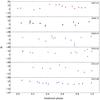 |
Fig. 1 Variability of the longitudinal field (Bl) as a function of the rotational phase. Each of the sub plots from top to bottom correspond to six different epochs (2007.67, 2008.71, 2009.54, 2010.62, 2011.67, and 2013.68). |
4. Mean longitudinal magnetic field (Bl)
The longitudinal magnetic field is measured using the LSD Stokes V and Stokes I profiles, where the field measured is the mean magnetic field (line of sight component) integrated over the entire visible stellar surface. The centre-of-gravity method (Rees & Semel 1979) was used on the LSD profile of HN Peg to measure its longitudinal magnetic field, as shown in Eq. (1), 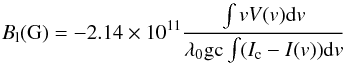 (1)where Bl is the longitudinal magnetic field in Gauss, λ0 = 550 nm is the central wavelength of the LSD profile, g = 1.21 is the Landé factor of the line list, c is the speed of light in km s-1, v is the radial velocity in km s-1 and Ic is the normalised continuum. The velocity range covered by the integration window is ± 17 km s-1 around the line centre. The uncertainty in each of the longitudinal magnetic field measurements are obtained by propagating the errors computed by the reduction pipeline in Eq. (1) as described by Marsden et al. (2014). The magnetic field from the LSD null profiles were also calculated for each observations where the magnetic field is approximately zero, indicating negligible spurious polarisation affect on the longitudinal field measurements. The errors in the longitudinal magnetic field of HN Peg is higher than the null profiles except in a few cases where the SN is weak compared to the rest of the observations. The magnetic field of HN Peg (Bl) and the magnetic field from the null profile and their related uncertainties are recorded in Table 4.
The variability of the longitudinal magnetic field of HN Peg as a function of rotational phase is shown in Fig. 1. The phase dependence of the longitudinal magnetic field indicates a complex surface magnetic field geometry. No long-term trend in mean longitudinal field measurements was observed for HN Peg as shown in Fig. 6, where Bl exhibits no significant long-term variations through out the observational timespan. The mean Bl value of 5.3 G with a dispersion of 4.2 G in epoch 2007.67 goes down to its lowest value of 1.9 G with a dispersion of 6.3 G in epoch 2009.54. The mean value is the highest in epoch 2010.62.
5. Chromospheric activity indicators
Chromospheric activity has been widely observed in solar type stars, which is manifested as emission in the line cores of the chromospheric lines, such as: Ca II H&K, Hα, and Ca II IRT lines. The varying flux in these line cores can be used as a proxy to investigate magnetic cycles.
5.1. S-index
We observe strong emission lines in the Ca II H&K line cores of HN Peg as a function of its rotational phase. The S-index is calculated by using two triangular band passes centred at Ca II H and K lines (Duncan et al. 1991; Morgenthaler et al. 2012) at 396.8469 and 393.3663 nm respectively with a FWHM of 0.1 nm. The flux in the continuum at the red and blue sides of the line is measured by using two 2 nm wide rectangular band passes R and V at 400.107 and 390.107 nm respectively. Equation (2) is used to calibrate our index with the Mount Wilson values, 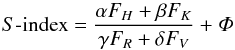 (2)where FH, FK, FR and FV are the flux in the band passes H,K,R and V. The NARVAL coefficients used to match our S-index values to the Mt Wilson values (Marsden et al. 2014) are α = 12.873, β = 2.502, γ = 8.877, δ = 4.271 and Φ = 1.183e - 03. We do not carry out the renormalisation procedure used by Morgenthaler et al. (2012) and carry out the continumm check following the procedure in Waite et al. (2014), where it was determined that removal of the overlapping orders is as efficient as renormalisation of the spectra.
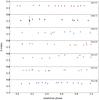 |
Fig. 2 Variability of S-index as a function of the rotational phase. Each of the sub plots from top to bottom correspond to seven different epochs (2007.67, 2008.71, 2009.54, 2010.62, 2011.67, 2012.61, and 2013.68). |
The variability of HN Peg’s S-index for each of the seven epochs is shown as a function of rotational phase in Fig. 2. The error in the S-index for each measurement was calculated using error propagation. The S-index and related uncertainty for each observation is shown in Table 4.
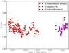 |
Fig. 3 S-index measurements of HN Peg from the combined data sets. The red circles represent data from the Mount Wilson survey, the black hexagons represent data from the CPS survey and the magenta squares are our measurements. |
We also included S-index measurements of HN Peg from the Mount Wilson survey, where the data was collected from 1966 to 1991 (Baliunas et al. 1995). There are no published S-index measurements of HN Peg from 1991 to 2004. Additional S-index values were obtained from the California planet search program Isaacson & Fischer (2010), two in 2004 and one in 2006. No error bars are available for the S-index measurements taken from literature. The long term S-index measurements from the combined data are shown in Fig. 3.
5.2. Hα-index
The rotational variation of the Hα line was also determined. A rectangular band pass of 0.36 nm width, centred at the Hα line at 656.285 nm (Gizis et al. 2002) and two 0.22 nm wide rectangular band passes Hblue and Hred at 655.77 and 656.0 nm respectively were used to measure the Hα-index. We corrected the order overlap in the NARVAL spectra and used the order containing the complete Hα line core. We then calculated the Hα-index using Eq. (3), 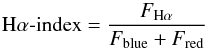 (3)where FHα represents the flux in the Hα line core and Fblue and Fred represent the flux in the continuum band pass filters Hblue and Hred respectively. The variability of Hα as a function of HN Peg’s rotational phase is shown in Fig. 4. The uncertainty in Hα-index measurements were calculated using error propagation. The Hα-index and related uncertainty for each observations are shown in Table 4.
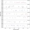 |
Fig. 4 Variability of the Hα-index as a function of rotational phase. Each of the sub plots from top to bottom correspond to seven different epochs (2007.67, 2008.71, 2009.54, 2010.62, 2011.67, 2012.61, and 2013.68). |
5.3. CaIRT-index
Since NARVAL covers a wide wavelength range from 350 nm up to 1000 nm, we can also observe the Ca II IR triplet lines. We take 0.2 nm wide rectangular band passes in the cores of each of the triplet lines at 849.8023 nm, 854.2091 nm and 866.241 nm. Two continuum band passes of the width of 0.5 nm are defined as IRred at 870.49 nm and IRblue at 847.58 nm for the flux at the red and blue sides of the IR lines (Petit et al. 2013). We calculate the CaIRT-index using Eq. (4), 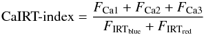 (4)where the flux in the three line cores are represented by FCa1, FCa2 and FCa3 respectively and the continuum fluxes are defined by FIRTblue and FIRTred respectively. The error bars for individual observations were calculated using error propagation. The variability of the CaIRT-index as a function of HN Peg’s rotational phase is shown in Fig. 5.
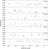 |
Fig. 5 Variability of CaIRT-index with the rotational phase. Each of the sub plots from top to bottom correspond to seven different epochs (2007.67, 2008.71, 2009.54, 2010.62, 2011.67, 2012.61, and 2013.68). |
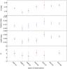 |
Fig. 6 Average value of the three different indices with the vertical bars showing the dispersion in each epoch of observations. Top to bottom: average values of S-index(red full circles), Hα-index (blue stars), CaIRT-index (black triangle) and Bl (magenta squares) plotted against the epochs (2007.67-2013.68) in average Julian dates. |
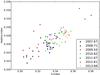 |
Fig. 7 Correlation between the S-index and Hα-index for each epoch of observations. |
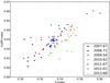 |
Fig. 8 Correlation between the S-index and CaIRT-index for each epoch of observations. |
The long-term variability over the observational epochs of this analysis for the three activity indicators: Ca II H&K, Hα, and Ca II IRT lines are shown in Fig. 6, where the mean values of each index is plotted as a function of the observational epochs. The error bars represent the standard deviation of the activity proxies for each epoch of observation. The long-term S-index variations are prominent than the rotationally induced variations. The long-term S-index and Hα-index show visible correlation over the entire time span of our observations. The two indices show a decreasing trend from 2007.67 to 2008.71 and show an increasing trend from 2008.71 to 2011.67 and then exhibits a flat trend. The long-term CaIRT-index measurements show global correlation with the S-index but shows more small-scale variations on a year-to-year basis.
The correlation between the different activity proxies for individual epochs is prominent in some epochs but not clearly visible in other epochs. The correlation between S-index and Hα-index throughout the entire observational timespan is shown in Fig. 7, where the correlation is more clearly visible. Correlation between S-index and CaIRT-index is shown in Fig. 8. The activity index measurements and their related uncertainties of HN Peg is tabulated in Table 4.
6. Large-scale magnetic field topology
The large-scale surface magnetic topology of HN Peg was reconstructed by using the Zeeman Doppler imaging (ZDI) tomographic technique, developed by Semel (1989); Brown et al. (1991); Donati & Brown (1997). ZDI technique involves solving an inverse problem and reconstructing the large-scale surface magnetic geometry by iteratively comparing the Stokes V profile to the synthetically generated profiles, which are generated from a synthetic stellar model.
Magnetic properties of HN Peg extracted from the ZDI maps.
The large-scale field geometry of HN Peg was reconstructed by using the version of ZDI that reconstructs the field into its toroidal and poloidal components, expressed as spherical harmonics expansion (Donati et al. 2006). A synthetic stellar model of HN Peg was constructed using 5000 grid points, where the local Stokes I profile in each grid cell was assumed to have a Gaussian shape and was adjusted to match the observed Stokes I profile. The synthetic local Stokes V profiles were computed under the weak field assumption and iteratively compared to the observed Stokes V profile. The maximum entropy approach adopted by the ZDI code is based on the algorithm of Skilling & Bryan (1984). In this implementation of the maximum entropy principle, a target value of the reduced χ2 is set by the user, where we define the reduced χ2 as the χ2 divided by the number of data points (Skilling & Bryan 1984). In its first series of iterations, the ZDI code produces magnetic models with associated synthetic profiles that progressively get closer to the target χ2 value. When the required reduced χ2 value is reached, new iterations increase the entropy of the model (at fixed χ2), converging step by step towards the magnetic model that minimises the total information of the magnetic map.
6.1. Radial velocity
The radial velocity of HN Peg was determined by fitting a Gaussian directly to the Stokes I profile to determine the centroid of the profile. This method was applied to each epoch of HN Peg. Additionally the radial velocity in our ZDI code was varied in 0.1 km s-1 steps. The radial velocity which results in the minimum information content was chosen which was comparable to the radial velocity obtained by Gaussian fit. The radial velocity and the associated uncertainty for each observational epoch is shown in Table 2.
6.2. Inclination angle
The inclination angle of 75° was inferred using the stellar parameters of HN Peg as shown in Table 1, which was tested within its error range by using as an input to the ZDI code. The inclination angle was increased in 5° steps and the inclination angle which resulted in minimum information content was used to generate the magnetic maps.
6.3. Differential rotation
The data used to reconstruct the magnetic field topology were collected over a span of several weeks, which might result into the introduction of latitudinal differential rotation during our timespan of observation. Differential rotation of HN Peg was measured by determining the difference in equatorial and polar shear incorporating a simplified solar-like differential rotation law into the imaging process:  (5)where Ω(l) is the rotation rate at latitude l, Ωeq is the equatorial rotation and dΩ is the difference in rotation between the equator and the poles.
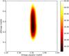 |
Fig. 9 Best fit χ2 map obtained by varying the parameters for 2007 data. The Ωeq and dΩ values obtained from this map are 1.36 rad d-1 and 0.22 rad d-1 respectively. |
For a given set of Ωeq and dΩ the large-scale magnetic field geometry was reconstructed, following the method of Petit et al. (2002). Approximately 15 observations with good phase coverage (Morgenthaler et al. 2012) is required to retrieve the parameters of the surface differential law. As good phase coverage is important to perform differential rotation calculations, the two epochs 2007.67 (14 observations) and 2013.68 (13 observations) were selected and individual differential rotation parameters were calculated. As shown in Fig. 9, the Ω and dΩ values for 2007.67 epoch are 1.36±0.01 rad d-1 and 0.22±0.03 rad d-1 and for 2013.68 epoch are 1.27±0.01 rad d-1 and 0.22±0.02 rad d-1 respectively. For the other epochs with less dense phase coverage the differential rotation values measured for 2007.67 are used for 2008.71, 2009.52 and values from 2013.68 are used for 2010.62 and 2011.67. The rotational period of HN Peg was also measured from the calculated differential rotational parameters.
The uncertainty in the differential rotation measurements were evaluated by obtaining Ωeq and dΩ values by varying the input stellar parameters, within the error bars of the individual parameters. The dispersion in the resulting values were considered as error bars.
6.4. Magnetic topology
The large-scale magnetic field topology of HN Peg was reconstructed using ZDI, for the epochs 2007.67, 2008.71, 2009.54, 2010.62, 2011.67, and 2013.68. The stellar parameters used to reconstruct the magnetic field topology are a vsini of 10.6 km s-1, an inclination angle of 75°. The number of spherical harmonics l used in our ZDI code is lmax = 8.
6.4.1. Epoch 2007.67
For the epoch 2007.67, the modelled Stokes V profile and the corresponding fit to the observed Stokes V profile is shown in Fig. 10 (Top left). The observed fit was achieved with a reduced χ2 of 1.0. The number of degree of freedom is 152. In the radial field component of the magnetic field as shown in Fig. 11, a strong positive field region is reconstructed at the equator along with a cap of positive polarity magnetic field encircling the pole. The azimuthal component is reconstructed as a band of positive magnetic field at equatorial latitudes as shown in Fig. 11. The percentage of the total magnetic energy distributed into its poloidal and toroidal configuration for the epoch 2007.67 is shown in Fig. 12. The magnetic energy is 57% poloidal and 43% toroidal as shown in Table 2. The percentage of the poloidal field reconstructed into its different components is shown in Fig. 13. The mean magnetic field strength of HN Peg is 18±0.5 G (Table 2).
 |
Fig. 10 Top row: time series of the LSD Stokes V profiles from 2007.67 (top left), 2008.71 (top centre) and 2009.54 (top right). Bottom row: time series of the LSD Stokes V profiles for the epochs 2010.62 (bottom left), 2011.67 (bottom centre) and 2013.68 (bottom right). The black line represents the observed Stokes V spectra and the red line represents the fit to the spectra. Rotational cycle is shown to the right and 1σ error bars for each observations is shown to the left for each plot. |
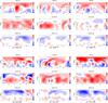 |
Fig. 11 Surface magnetic field geometry of HN Peg for six epochs as reconstructed using Zeeman Doppler Imaging. Top row: a) 2007.67; b) 2008.71; c) 2009.54; bottom row: d) 2010.62; e) 2011.67; f) 2013.68. For each epoch, the magnetic field components are shown as projection onto one axis of the spherical coordinate frame, where from top to bottom: radial, azimuthal and meridional magnetic field components are shown. the field strength is shown in Gauss, where red represents positive polarity and blue represents negative polarity. |
6.4.2. Epoch 2008.71
The LSD Stokes V profile and the corresponding fit for the epoch 2008.71 is shown in Fig. 10 (top middle). The observed fit was achieved with a χ2 minimised to 1.0 and the number of degree of freedom is 68. The radial field geometry is dominated by a positive magnetic region over the poles as shown in Fig. 11, where the strong positive field at the equator in epoch 2007.67 is not visible one year later in epoch 2008.71. The azimuthal field geometry is dominated by two regions of positive polarity at the equator. The meridional field geometry is also shown in Fig. 11. The percentage of the total magnetic energy distributed into the poloidal and toroidal components is shown in Fig. 12. The majority of the magnetic energy is reconstructed as toroidal field component as shown in Table 2. The percentage of fraction of the poloidal magnetic field reconstructed into its different components is shown in Fig. 13. The mean magnetic field strength decreases to 14±0.3 G (Table 2).
6.4.3. Epoch 2009.54
The Stokes V profile in 2009.54 is shown in Fig. 10 (top right), where some of the Stokes V profile have a lower S/N. The Stokes V profiles are fitted to the reconstructed profile with a χ2 level of 1.0 and the number of degree of freedom is 40. The positive polarity magnetic region around the pole in the previous epochs is also present in 2009.54 as shown in Fig. 11. The band of positive polarity azimuthal field observed in the previous epochs is surprisingly absent in this epoch as shown in Fig. 11, with only 11% of the magnetic energy being toroidal. The percentage of magnetic energy reconstructed as poloidal component is 89% as shown in Fig. 12. The percentage of the fraction of the poloidal magnetic energy distributed into its different field configurations is shown in Fig. 13. The mean magnetic field strength is at its lowest at 11±0.2 G. (Table 2).
6.4.4. Epoch 2010.62
The Stokes V profile and magnetic maps of HN Peg for epoch 2010.62 are shown in Fig. 10 (bottom left) and Fig. 11 respectively. The best fit to the observed Stokes V profiles were obtained with a χ2 level of 1.4, which might be a result of some intrinsic behaviour that could not be accounted for. The number of degree of freedom is 40. The radial field component is still mostly positive around the poles as shown in Fig. 11. The azimuthal field is stronger than in epoch 2009.54, with the presence of both positive and negative polarity regions. The meridional field component is also shown in Fig. 11. The percentage of the magnetic energy distribution into its poloidal and toroidal component is shown in Fig. 12. 65% of the magnetic energy is reconstructed in the poloidal component and 35% of the energy is stored in the toroidal component as shown in Table 2. The percentage of the fraction of the poloidal component reconstructed into its different components is shown in Fig. 13, where the fraction of the different components is minimal. The mean magnetic field strength of HN Peg has increased from 11±0.2 G in 2009.54 to 19±0.8 G (Table 2).
6.4.5. Epoch 2011.67
For the epoch 2011.67, the reconstructed Stokes V profile and its fit to the observed Stokes V profile is shown in Fig. 10 (bottom middle). The observed fit was obtained with a χ2 minimised to 1.1. The formal computation of the number of degree of freedom for this epoch results in a negative value, which means for this particular case the problem is underdetermined. The magnetic field geometry in the radial field is more complex than in the previous epochs, with the presence of both positive and negative magnetic regions as shown in Fig. 11. However, the phase coverage is not sufficient to reliably confirm the negative polarity regions. The azimuthal field is mostly positive with regions of positive polarity around the equator. The meridional field is also shown in Fig. 11. The percentage of the magnetic energy distributed into the poloidal and toroidal components is shown in Fig. 12. The percentage of the fraction of the poloidal component reconstructed into its different field configurations is shown in Fig. 13. 61% of the magnetic energy is reconstructed into its poloidal component as shown in Table 2, where the mean magnetic field strength of HN Peg is 19±0.7 G.
6.4.6. Epoch 2013.68
The observed and reconstructed Stokes V profiles for the epoch 2013.68 is shown in Fig. 10 (bottom right). The best fit to the observed Stokes V profiles was obtained with a χ2 of 1.0. The number of degree of freedom is 124. The magnetic field in the radial component is shown in Fig. 11, where the pole is dominated with a ring of positive polarity magnetic field. The azimuthal field component is dominated by a band of positive polarity magnetic field at the equator as shown in Fig. 11. The percentage of the magnetic energy distributed into different field configurations is shown in Fig. 12. The magnetic energy is mostly poloidal (62%) as shown in Table 2. The percentage of the fraction of poloidal field reconstructed into its different configurations is shown in Fig. 13. The mean magnetic field is at its highest at 24±0.7 G, where 77% of the total field is axisymmetric (Table 2).
The uncertainties associated with the magnetic maps for each epoch of observations were obtained by using different values for the input stellar parameters into our ZDI code (see Petit et al. 2002), where the individual parameters were varied within their error bars. The dispersion in the resulting values was considered as error bars.
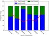 |
Fig. 12 Magnetic energy distribution throughout the six epochs (2007.67, 2008.71, 2009.54, 2010.62, 2011.67, and 2013.68). The fraction of magnetic field stored in poloidal component is shown in blue and toroidal component in green.The red line represents the fraction of the energy stored in the axisymmetric component. The error bars associated with each epoch are shown in Table 2. |
7. Discussion
HN Peg was observed for seven epochs from 2007.67 to 2013.68, providing new insights into its magnetic field variations and the associated geometry.
7.1. Long-term magnetic variability
The longitudinal magnetic field (Bl) for each observation of HN Peg was derived using Stokes V profile and Stokes I profile integrated over the entire visible stellar surface. The longitudinal field varies as a function of the rotational phase during each observational epoch, which indicates a non-axisymmetric magnetic geometry. Over the epochs of this analysis no significant long-term Bl variations are apparent as shown in Fig. 6, where the mean Bl values exhibit variability over the observational timespan but the overall trend with dispersion is flat. HN Peg exhibits a strong longitudinal magnetic field strength when compared to the other solar type stars included in Marsden et al. (2014). Bl ranges from −14 G up to 13 G (Table 4) throughout the entire time span.
The long term chromospheric variability of HN Peg was monitored using three different chromospheric lines: Ca II H&K, Hα and Ca II IRT. The three chromospheric tracers exhibit weak rotational dependence during each observational epoch. Periodic analysis of HN Peg carried out by the Mount Wilson survey categorised HN Peg as a variable star with a period of 6.2±0.2 years. The chromospheric activity of HN Peg was also measured as part of the Bcool snapshot survey (Marsden et al. 2014), where the measured S-index are compatible with our S-index measurements.
Correlations were observed for the three chromospheric tracers for individual epochs with visible scatter, which might be due to the effect of different temperature and pressure conditions during emissions in the line cores of Ca II H&K, Hα, and Ca II IRT. Correlations between S-index and Hα-index were also observed for ξ Bootis A by Morgenthaler et al. (2012). The observed scatter in the correlation between S-index and Hα-index for each epoch might be also be explained by the contribution of plage variation in Ca II H&K and filament variation in Hα flux (Meunier & Delfosse 2009), where increase in filament contribution might result in decrease in correlation between the two chromospheric tracers. Apart from the contribution of filament and plage, Meunier & Delfosse (2009) also concluded that stellar inclination angle, phase coverage might also effect the correlation between these two tracers.
In their long-term evolution, the chromospheric tracers exhibit a similar trend, with visible correlation between the S-index and Hα-index. In the long-term mean S-index and Hα-index exhibit correlation in cool stars, which might be due to the effect of stellar colour (Cincunegui et al. 2007). The long-term Ca II H&K and Hα correlation is clearly observed in the Sun (Livingston et al. 2007), where the two activity proxies follow the solar magnetic cycle. This long-term correlation between these two tracers have also been observed in other cool stars with high activity index (Gomes da Silva et al. 2014).
For each observational epoch no visible correlation is observed between the variability of the longitudinal magnetic field and the chromospheric tracers. Correlations between the direct field measurements and the magnetic activity proxies were also not observed for the solar analogue ξ Bootis A (Morgenthaler et al. 2012). This lack of correlation can be explained by the contribution of small scale magnetic features in chromospheric activity measurements which are lost in the polarised Stokes V magnetic field calculations due to magnetic flux cancellations.
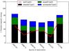 |
Fig. 13 Poloidal magnetic field distributed into different configurations throughout the six epochs (2007.67, 2008.71, 2009.54, 2010.62, 2011.67, and 2013.68). The fraction of the poloidal magnetic energy stored as dipole is shown in black, quadrupole in green and octopole in blue. The red line represents the fraction of the poloidal energy stored in the axisymmetric component. The error bars associated with each epoch are shown in Table 2. |
7.2. Large scale magnetic topology
The large-scale magnetic topology of HN Peg was reconstructed for six observational epochs (2007.67, 2008.71, 2009.54, 2010.62, 2011.67, and 2013.68), where the mean magnetic field strength (Bmean) changes with the geometry of the field from epoch-to-epoch. The mean magnetic field strength of HN Peg is of a few G, which is considerably smaller when compared to the mean magnetic field of other solar analogues HD 189733 (1.34 ± 0.13 M⊙, Teff = 6014 K; Fares et al. 2010) and ξ Bootis A (0.86±0.07 M⊙, Teff = 5551 ± 20; Morgenthaler et al. 2012). The mean magnetic field strength of HN Peg is higher than HD 190771, which has a mass of 0.96±0.13 M⊙ and Teff of 5834±50 (Petit et al. 2009; Morgenthaler et al. 2011). When compared to solar-type stars of similar spectral type HN Peg exhibits higher mean field strength than the mean field strength of τ Boo(F7) with a mass of 1.33±0.11M⊙ (Fares et al. 2009), HD 179949(F8) (Fares et al. 2012), where τ Boo and HD 179949 are both planet hosting stars.
The radial field component of HN Peg exhibits a variable field geometry, where the field strength varies from epoch-to-epoch as shown in Fig. 11. A positive polarity region at the pole is observed in epoch 2007.67, where a strong positive polarity magnetic region is also observed near the equator. The positive region at the pole is present throughout our observational epoch, without exhibiting any polarity switch. The magnetic field energy is stored into its poloidal and toroidal components. The poloidal field of HN Peg is not a simple dipole. The fraction of energy stored into the different components of the poloidal field exhibits variations from epoch-to-epoch as shown in Fig. 13.
The azimuthal field component of HN Peg exhibits a more variable geometry compared to the radial field geometry. The azimuthal field component exhibits the presence of a significant positive polarity magnetic regions, which undergoes variations from epoch-to-epoch as shown in Fig. 11. A strong positive polarity band of magnetic field encircling the star is observed in epoch 2007.67. In 2008.71 two strong positive polarity magnetic regions were observed near the equator. The azimuthal component becomes negligible in the epoch 2009.54. The toroidal field percentage is minimum in epoch 2009.54. The azimuthal field reappears in 2010.62, where opposite polarity magnetic field regions are observed. In 2011.67 stronger positive polarity regions are observed, which finally appears as a toroidal ring in epoch 2013.68.
Prominent toroidal features have been observed in a wide range of stars belonging to different spectral class, such as HD 190771 (Petit et al. 2009), ξ Bootis A (Morgenthaler et al. 2012), τ Boo (Fares et al. 2009) and HD 189733 (Fares et al. 2010). The sudden disappearance of the toroidal field was also observed in ξ Boo (Morgenthaler et al. 2012). The toroidal component is prominent in solar-type stars with rotation periods as short as a few days (Petit et al. 2008) and stars with longer rotational periods show more prominent poloidal component, which is clearly observed in the Sun. Toroidal band was also not observed in the F8 dwarf HD 179949 (Fares et al. 2012), where only two epochs of observations were available. The presence of significant global-scale toroidal field has also been observed in numerical simulations of rapidly rotating suns (Brown et al. 2010), where the surface field topology becomes predominantly toroidal for stars with rotation periods of a few days.
No polarity switches have been observed for HN Peg, although it showed significant evolution of its magnetic field geometry over the span of six observational epochs. Magnetic cycles were also not observed for ξ Bootis A and HD 189733, which are slower rotators when compared to HN Peg. Polarity switches were observed in HD 190771, τ Boo and HD 78366 over their observational time span. Magnetic cycles shorter than the magnetic cycle of the Sun were observed for τ Boo and HD 78366.
The variability of the mean magnetic field of HN Peg follows a similar trend as that of the toroidal field component (Table 2). The mean magnetic field (Bmean) of HN Peg show a gradual decrease in its field strength from 2007.67 to 2009.54, with minimum Bmean in 2009.54. The mean field starts increasing from 2009.54 till it reaches a maximum strength in 2013.68. This indicates strong dependence of the mean field strength on the toroidal component of the magnetic field.
7.3. Differential rotation
HN Peg has a low vsini of 10.6 km s-1, which makes it unsuitable for differential rotation calculations using other conventional techniques such as line profile studies using Fourier Transform method (Reiners & Schmitt 2003). Photometric observations of HN Peg were used to measure its differential rotation by Messina & Guinan (2003), where the evolution of the rotation of the star along the star spot cycle was measured with inconclusive results.
The differential rotation of HN Peg was calculated using Stokes V and I profiles in the ZDI technique. Two epochs with the best phase coverage were used (2007.67 and 2013.68) in our differential rotation calculations. The Ω and dΩ values for 2007.67 epoch were 1.36 ± 0.01 rad d-1 and 0.22 ± 0.03 rad d-1 and for 2013.68 epoch were 1.27 ± 0.01 rad d-1 and 0.22 ± 0.02 rad d-1 respectively.
HN Peg exhibits weak differential rotation compared to other dwarfs of similar spectral types such as HD 171488 (G0) (Stokes I/Stokes V: Ωeq = 4.93 ± 0.05 / 4.85 ± 0.05 rad d-1, dΩ = 0.52 ± 0.04 / 0.47 ± 0.04 rad d-1; Jeffers & Donati 2008) and τBoo(F7) (2008 June: Ωeq = 2.05 ± 0.04 rad d-1 and dΩ = 0.42 ± 0.10 rad d-1 rad d-1, 2008 July: Ωeq = 2.12 ± 0.12 rad d-1 and dΩ = 0.50 ± 0.15 rad d-1; Fares et al. 2009). HD 171488 is the closest to HN Peg in terms of spectral type, stellar radius and age. The dΩ values of HN Peg is higher than the other young early G dwarfs such as LQ Lup (Ωeq = 20.28 ± 0.01 rad d-1, dΩ = 0.12 ± 0.02 rad d-1; Donati et al. 2000) and R58 (2000 January: Ωeq = 11.14 ± 0.01 and dΩ = 0.03 ± 0.02, 2003 March: Ωeq = 11.19 ± 0.01 and dΩ = 0.14 ± 0.01; Marsden et al. 2004). When compared to HD 179949(Ωeq = 0.82 ± 0.01 rad d-1, dΩ = 0.22 ± 0.06 rad d-1; Fares et al. 2012), HN Peg exhibits comparable dΩ values. Although, when compared to other fast rotators such as ξ Boo (Prot = 6.43 days; Morgenthaler et al. 2012), HN Peg exhibits weaker differential rotation. No direct correlation between differential rotation of HN Peg and solar analogues of similar stellar parameters such as age, spectral type, Prot have been observed so far.
8. Summary
In this paper we presented the large-scale magnetic topology of the young solar analogue HN Peg. HN Peg is a variable young dwarf with a complex magnetic geometry, where the radial field exhibits stable positive polarity magnetic field region through out our observational epochs. In contrast, the azimuthal field exhibits a highly variable geometry where a band of positive polarity toroidal field is observed in the first epoch of observation followed by a negligible toroidal field two years later in epoch 2009.54. The toroidal band emerges again one year later in epoch 2010.62 which is stable in the later epochs 2011.67 and 2013.68. The long-term longitudinal magnetic field variations were also calculated where in the long-term the longitudinal field exhibits a flat trend. The chromospheric activity was also measured, where the chromospheric activity indicators exhibit a long-term correlation.
Online material
Journal of observations for seven epochs (2007−2013).
The chromospheric activity measurements and magnetic field measurements of HN Peg for seven epochs (2007.67, 2008.71, 2009.54, 2010.62, 2011.67, 2012.61 and 2013.68).
A detailed description of the polarisation defects and the correction technique used can be found here: http://spiptbl.bagn.obs-mip.fr/Actualites/Anomalies-de-mesures
Acknowledgments
This work was carried out as part of Project A16 funded by the Deutsche Forschungdgemeinschaft (DFG) under SFB 963. Part of this work was also supported by the COST Action MP1104 “Polarisation as a tool to study the Solar System and beyond”.
References
- Aurière, M. 2003, in EAS Publ. Ser. 9, eds. J. Arnaud, & N. Meunier, 105 [Google Scholar]
- Baliunas, S. L., Horne, J. H., Porter, A., et al. 1985, ApJ, 294, 310 [NASA ADS] [CrossRef] [Google Scholar]
- Baliunas, S. L., Donahue, R. A., Soon, W. H., et al. 1995, ApJ, 438, 269 [NASA ADS] [CrossRef] [Google Scholar]
- Barnes, S. A. 2007, ApJ, 669, 1167 [NASA ADS] [CrossRef] [Google Scholar]
- Brandenburg, A., & Subramanian, K. 2005, Phys. Rep., 417, 1 [NASA ADS] [CrossRef] [Google Scholar]
- Brown, B. P., Browning, M. K., Brun, A. S., Miesch, M. S., & Toomre, J. 2010, ApJ, 711, 424 [Google Scholar]
- Brown, S. F., Donati, J.-F., Rees, D. E., & Semel, M. 1991, A&A, 250, 463 [NASA ADS] [Google Scholar]
- Catala, C., Donati, J.-F., Shkolnik, E., Bohlender, D., & Alecian, E. 2007, MNRAS, 374, L42 [NASA ADS] [CrossRef] [Google Scholar]
- Charbonneau, P. 2010, Liv. Rev. Sol. Phys., 7, 3 [Google Scholar]
- Cincunegui, C., Díaz, R. F., & Mauas, P. J. D. 2007, A&A, 469, 309 [NASA ADS] [CrossRef] [EDP Sciences] [Google Scholar]
- Donati, J.-F., & Brown, S. F. 1997, A&A, 326, 1135 [NASA ADS] [Google Scholar]
- Donati, J.-F., & Landstreet, J. D. 2009, ARA&A, 47, 333 [NASA ADS] [CrossRef] [MathSciNet] [Google Scholar]
- Donati, J.-F., Semel, M., Carter, B. D., Rees, D. E., & CollierCameron, A. 1997, MNRAS, 291, 658 [NASA ADS] [CrossRef] [MathSciNet] [Google Scholar]
- Donati, J.-F., Mengel, M., Carter, B. D., et al. 2000, MNRAS, 316, 699 [NASA ADS] [CrossRef] [Google Scholar]
- Donati, J.-F., Collier Cameron, A., Semel, M., et al. 2003, MNRAS, 345, 1145 [NASA ADS] [CrossRef] [Google Scholar]
- Donati, J.-F., Howarth, I. D., Jardine, M. M., et al. 2006, MNRAS, 370, 629 [NASA ADS] [CrossRef] [Google Scholar]
- Duncan, D. K., Vaughan, A. H., Wilson, O. C., et al. 1991, ApJS, 76, 383 [NASA ADS] [CrossRef] [Google Scholar]
- Eisenbeiss, T., Ammler- von Eiff, M., Roell, T., et al. 2013, A&A, 556, A53 [NASA ADS] [CrossRef] [EDP Sciences] [Google Scholar]
- Ertel, S., Wolf, S., Marshall, J. P., et al. 2012, A&A, 541, A148 [NASA ADS] [CrossRef] [EDP Sciences] [Google Scholar]
- Fares, R., Donati, J.-F., Moutou, C., et al. 2009, MNRAS, 398, 1383 [NASA ADS] [CrossRef] [MathSciNet] [Google Scholar]
- Fares, R., Donati, J.-F., Moutou, C., et al. 2010, MNRAS, 406, 409 [NASA ADS] [CrossRef] [Google Scholar]
- Fares, R., Donati, J.-F., Moutou, C., et al. 2012, MNRAS, 423, 1006 [NASA ADS] [CrossRef] [Google Scholar]
- Frasca, A., Freire Ferrero, R., Marilli, E., & Catalano, S. 2000, A&A, 364, 179 [NASA ADS] [Google Scholar]
- Fuhrmann, K. 2004, Astron. Nachr., 325, 3 [NASA ADS] [CrossRef] [MathSciNet] [Google Scholar]
- Gaidos, E. J. 1998, PASP, 110, 1259 [NASA ADS] [CrossRef] [Google Scholar]
- Gizis, J. E., Reid, I. N., & Hawley, S. L. 2002, AJ, 123, 3356 [NASA ADS] [CrossRef] [Google Scholar]
- Gomes da Silva, J., Santos, N. C., Boisse, I., Dumusque, X., & Lovis, C. 2014, A&A, 566, A66 [NASA ADS] [CrossRef] [EDP Sciences] [Google Scholar]
- Hall, J. C., Lockwood, G. W., & Skiff, B. A. 2007, AJ, 133, 862 [NASA ADS] [CrossRef] [Google Scholar]
- Isaacson, H., & Fischer, D. 2010, ApJ, 725, 875 [NASA ADS] [CrossRef] [Google Scholar]
- Jeffers, S. V., & Donati, J.-F. 2008, MNRAS, 390, 635 [NASA ADS] [CrossRef] [Google Scholar]
- Kochukhov, O., Makaganiuk, V., & Piskunov, N. 2010, A&A, 524, A5 [NASA ADS] [CrossRef] [EDP Sciences] [Google Scholar]
- Leggett, S. K., Saumon, D., Albert, L., et al. 2008, ApJ, 682, 1256 [NASA ADS] [CrossRef] [Google Scholar]
- Livingston, W., Wallace, L., White, O. R., & Giampapa, M. S. 2007, ApJ, 657, 1137 [NASA ADS] [CrossRef] [Google Scholar]
- López-Santiago, J., Montes, D., Crespo-Chacón, I., & Fernández-Figueroa, M. J. 2006, ApJ, 643, 1160 [NASA ADS] [CrossRef] [Google Scholar]
- Luhman, K. L., Patten, B. M., Marengo, M., et al. 2007, ApJ, 654, 570 [NASA ADS] [CrossRef] [Google Scholar]
- Marsden, S. C., Waite, I. A., Carter, B. D., & Donati, J.-F. 2004, Astron. Nachr., 325, 246 [NASA ADS] [CrossRef] [Google Scholar]
- Marsden, S. C., Petit, P., Jeffers, S. V., et al. 2014, MNRAS, 444, 3517 [NASA ADS] [CrossRef] [Google Scholar]
- Messina, S., & Guinan, E. F. 2002, A&A, 393, 225 [Google Scholar]
- Messina, S., & Guinan, E. F. 2003, A&A, 409, 1017 [NASA ADS] [CrossRef] [EDP Sciences] [Google Scholar]
- Meunier, N., & Delfosse, X. 2009, A&A, 501, 1103 [NASA ADS] [CrossRef] [EDP Sciences] [Google Scholar]
- Morgenthaler, A., Petit, P., Morin, J., et al. 2011, Astron. Nachr., 332, 866 [NASA ADS] [CrossRef] [Google Scholar]
- Morgenthaler, A., Petit, P., Saar, S., et al. 2012, A&A, 540, A138 [NASA ADS] [CrossRef] [EDP Sciences] [Google Scholar]
- Parker, E. N. 1955, ApJ, 122, 293 [NASA ADS] [CrossRef] [Google Scholar]
- Petit, P., Donati, J.-F., & Collier Cameron, A. 2002, MNRAS, 334, 374 [NASA ADS] [CrossRef] [MathSciNet] [Google Scholar]
- Petit, P., Dintrans, B., Solanki, S. K., et al. 2008, MNRAS, 388, 80 [NASA ADS] [CrossRef] [MathSciNet] [Google Scholar]
- Petit, P., Dintrans, B., Morgenthaler, A., et al. 2009, A&A, 508, L9 [NASA ADS] [CrossRef] [EDP Sciences] [Google Scholar]
- Petit, P., Aurière, M., Konstantinova-Antova, R., et al. 2013, in Lect. Notes Phys. 857, eds. J.-P. Rozelot, & C. Neiner (Berlin: Springer Verlag), 231 [Google Scholar]
- Rees, D. E., & Semel, M. D. 1979, A&A, 74, 1 [NASA ADS] [Google Scholar]
- Reiners, A., & Schmitt, J. H. M. M. 2003, A&A, 398, 647 [NASA ADS] [CrossRef] [EDP Sciences] [Google Scholar]
- Schröder, K.-P., Mittag, M., Hempelmann, A., González-Pérez, J. N., & Schmitt, J. H. M. M. 2013, A&A, 554, A50 [NASA ADS] [CrossRef] [EDP Sciences] [Google Scholar]
- Semel, M. 1989, A&A, 225, 456 [NASA ADS] [Google Scholar]
- Skilling, J., & Bryan, R. K. 1984, MNRAS, 211, 111 [NASA ADS] [CrossRef] [Google Scholar]
- Valenti, J. A., & Fischer, D. A. 2005, VizieR Online Data Catalog, 215, 90141 [NASA ADS] [Google Scholar]
- Waite, I., Marsden, S. C., Carter, B. C., et al. 2014, MNRAS, submitted [Google Scholar]
- Wright, J. T., Marcy, G. W., Butler, R. P., & Vogt, S. S. 2004, ApJS, 152, 261 [NASA ADS] [CrossRef] [Google Scholar]
- Zuckerman, B., & Song, I. 2009, A&A, 493, 1149 [NASA ADS] [CrossRef] [EDP Sciences] [Google Scholar]
All Tables
The chromospheric activity measurements and magnetic field measurements of HN Peg for seven epochs (2007.67, 2008.71, 2009.54, 2010.62, 2011.67, 2012.61 and 2013.68).
All Figures
|
Fig. 1 Variability of the longitudinal field (Bl) as a function of the rotational phase. Each of the sub plots from top to bottom correspond to six different epochs (2007.67, 2008.71, 2009.54, 2010.62, 2011.67, and 2013.68). |
| In the text | |
|
Fig. 2 Variability of S-index as a function of the rotational phase. Each of the sub plots from top to bottom correspond to seven different epochs (2007.67, 2008.71, 2009.54, 2010.62, 2011.67, 2012.61, and 2013.68). |
| In the text | |
|
Fig. 3 S-index measurements of HN Peg from the combined data sets. The red circles represent data from the Mount Wilson survey, the black hexagons represent data from the CPS survey and the magenta squares are our measurements. |
| In the text | |
|
Fig. 4 Variability of the Hα-index as a function of rotational phase. Each of the sub plots from top to bottom correspond to seven different epochs (2007.67, 2008.71, 2009.54, 2010.62, 2011.67, 2012.61, and 2013.68). |
| In the text | |
|
Fig. 5 Variability of CaIRT-index with the rotational phase. Each of the sub plots from top to bottom correspond to seven different epochs (2007.67, 2008.71, 2009.54, 2010.62, 2011.67, 2012.61, and 2013.68). |
| In the text | |
|
Fig. 6 Average value of the three different indices with the vertical bars showing the dispersion in each epoch of observations. Top to bottom: average values of S-index(red full circles), Hα-index (blue stars), CaIRT-index (black triangle) and Bl (magenta squares) plotted against the epochs (2007.67-2013.68) in average Julian dates. |
| In the text | |
|
Fig. 7 Correlation between the S-index and Hα-index for each epoch of observations. |
| In the text | |
|
Fig. 8 Correlation between the S-index and CaIRT-index for each epoch of observations. |
| In the text | |
|
Fig. 9 Best fit χ2 map obtained by varying the parameters for 2007 data. The Ωeq and dΩ values obtained from this map are 1.36 rad d-1 and 0.22 rad d-1 respectively. |
| In the text | |
|
Fig. 10 Top row: time series of the LSD Stokes V profiles from 2007.67 (top left), 2008.71 (top centre) and 2009.54 (top right). Bottom row: time series of the LSD Stokes V profiles for the epochs 2010.62 (bottom left), 2011.67 (bottom centre) and 2013.68 (bottom right). The black line represents the observed Stokes V spectra and the red line represents the fit to the spectra. Rotational cycle is shown to the right and 1σ error bars for each observations is shown to the left for each plot. |
| In the text | |
|
Fig. 11 Surface magnetic field geometry of HN Peg for six epochs as reconstructed using Zeeman Doppler Imaging. Top row: a) 2007.67; b) 2008.71; c) 2009.54; bottom row: d) 2010.62; e) 2011.67; f) 2013.68. For each epoch, the magnetic field components are shown as projection onto one axis of the spherical coordinate frame, where from top to bottom: radial, azimuthal and meridional magnetic field components are shown. the field strength is shown in Gauss, where red represents positive polarity and blue represents negative polarity. |
| In the text | |
|
Fig. 12 Magnetic energy distribution throughout the six epochs (2007.67, 2008.71, 2009.54, 2010.62, 2011.67, and 2013.68). The fraction of magnetic field stored in poloidal component is shown in blue and toroidal component in green.The red line represents the fraction of the energy stored in the axisymmetric component. The error bars associated with each epoch are shown in Table 2. |
| In the text | |
|
Fig. 13 Poloidal magnetic field distributed into different configurations throughout the six epochs (2007.67, 2008.71, 2009.54, 2010.62, 2011.67, and 2013.68). The fraction of the poloidal magnetic energy stored as dipole is shown in black, quadrupole in green and octopole in blue. The red line represents the fraction of the poloidal energy stored in the axisymmetric component. The error bars associated with each epoch are shown in Table 2. |
| In the text | |
Current usage metrics show cumulative count of Article Views (full-text article views including HTML views, PDF and ePub downloads, according to the available data) and Abstracts Views on Vision4Press platform.
Data correspond to usage on the plateform after 2015. The current usage metrics is available 48-96 hours after online publication and is updated daily on week days.
Initial download of the metrics may take a while.