© ESO, 2014

1. Introduction

Despite considerable progress in the field of planet formation in recent years, many aspects are still far from understood (see Armitage 2011, for a review). It is clear that the initial conditions play an important role in the outcome of the planet formation process. Circumstellar disks, consisting of dust and gas, which orbit young stars are widely known to be the birth places of planets. One of the key properties for understanding how disks evolve to planetary systems is their overall mass, combined with their surface density distribution.

So far, virtually all disk mass determinations are based on observations of the millimeter (mm) continuum emission from dust grains (e.g., Beckwith et al. 1990; Dutrey et al. 1996; Mannings & Sargent 1997; Andrews & Williams 2005) (see Williams & Cieza 2011, for a review). To derive the total gas + dust disk mass from these data involves several steps and assumptions. First, a dust opacity value κ_ν at the observed frequency ν together with a dust temperature needs to be chosen to infer the total dust mass. The submillimeter dust opacity has been calibrated for dense cores against infrared extinction maps (Shirley et al. 2011) and found to agree well with theoretical opacities for coagulated grains with thin ice mantles (Ossenkopf & Henning 1994), but the dust grains in protoplanetary disks have probably grown to larger sizes with corresponding lower opacities at sub-mm wavelengths (e.g., Testi et al. 2003; Rodmann et al. 2006; Lommen et al. 2009; Ricci et al. 2010). These opacities may even vary with radial distance from the star, which adds another uncertainty (Guilloteau et al. 2011; Pérez et al. 2012; Birnstiel et al. 2012) (see Testi et al. 2014, for review). Second, a dust-to-gas mass ratio has to be assumed, which is usually taken to be the same as the interstellar ratio of 100. This conversion implicitly assumes that the gas and mm-sized dust grains have the same distribution. There is now growing observational evidence that mm-sized dust and gas can have very different spatial distributions in disks (e.g., Panić & Hogerheijde 2009; Andrews et al. 2012; van der Marel et al. 2013; Bruderer et al. 2014; Walsh et al. 2014), which invalidates the use of mm continuum data to trace the gas.

The alternative method for deriving disk masses relies on observations of the gas. The dominant constituent, H₂, is very difficult to observe directly because of its intrinsically weak lines at near- and mid-infrared wavelengths superposed on a strong continuum (e.g., Thi et al. 2001; Pascucci et al. 2006; Carmona et al. 2008; Bitner et al. 2008; Bary et al. 2008). Even if detected, H₂ does not trace the bulk of the disk mass in most cases (e.g., Pascucci et al. 2013). HD is a good alternative probe, but its far-infrared lines have so far been detected for only one disk (Bergin et al. 2013), and there is no current facility sensitive enough for deep searches in other disks after Herschel.

This leaves CO as the best, and probably only, alternative to determine the gas content of disks. In contrast with H₂ and HD, its pure rotational transitions at millimeter wavelengths are readily detected with a high signal-to-noise ratio in virtually all protoplanetary disks (e.g., Dutrey et al. 1996; Thi et al. 2001; Dent et al. 2005; Panić et al. 2008; Williams & Best 2014). It is the second-most abundant molecule after H₂, with a chemistry that is in principle well understood. However, ¹²CO is a poor tracer of the bulk of the gas mass because its lines become optically thick at the disk surface. Less abundant CO isotopologues such as ¹³CO and C¹⁸O have more optically thin lines and as a consequence saturate deeper in the disk, with C¹⁸O probing down to the midplane (van Zadelhoff et al. 2001; Dartois et al. 2003). Therefore, the combination of several isotopologues can be used to investigate both the radial and vertical gas structure of the disk. With the advent of the Atacama Large Millimeter/submillimeter Array (ALMA¹), high angular resolution observations of CO isotopologues in disks will become routine even for low-mass disks (e.g., Kóspál et al. 2013), allowing studies of the distribution of the cold (<100 K) gas in disks in much more detail than possible before. The ALMA data complement near-infrared vibration-rotation lines of CO, which mostly probe the warm gas in the inner few AU of the disk (e.g., Najita et al. 2003; Pontoppidan et al. 2008; Brittain et al. 2009; van der Plas et al. 2009; Brown et al. 2013).

The two main unknowns in the determination of the disk gas mass are the CO-H₂ abundance ratio and the isotopologue ratios. In the simplest situation, the bulk of the volatile carbon (i.e., the carbon that is not locked up refractory dust) is contained in gas-phase CO, leading to a CO/H₂ fractional abundance of ~ 2 × 10^-4, consistent with a direct observation of this abundance in a warm dense cloud (Lacy et al. 1994). The isotopologue ratios are then usually taken to be constant at the ¹³C, ¹⁸O, and ¹⁷O isotope values found in the local interstellar medium (ISM) (Wilson & Rood 1994). In reality, two processes act to decrease the CO abundance below its highest value: photodissociation and freeze-out. Photodissociation is effective in the surface layers of the disk, whereas freeze-out occurs in the cold (T_d< 20 K) outer parts of the disk at the midplane. Indeed, a combination of both processes has been invoked to explain the low observed abundances of CO in disks compared with H₂ masses derived from dust observations (Dutrey et al. 1997; van Zadelhoff et al. 2001; Andrews et al. 2011). An additional effect is that the volatile carbon abundance and [C]/[O] ratio in the disk can be different from that in warm clouds (Öberg et al. 2011; Bruderer et al. 2012) and affect the CO abundance. Indeed, a recent study by Favre et al. (2013) of the one disk, TW Hya, for which the mass has been determined independently using HD far-infrared lines, finds a low C¹⁸O abundance and consequently a low overall carbon abundance, which the authors interpreted as due to conversion of gas-phase CO to other hydrocarbons. These other carbon-bearing species have a stronger binding energy to the grains than CO itself, and freeze-out rapidly preventing conversion back to CO (Bergin et al. 2014).

Of these processes, only photodissociation by ultraviolet (UV) photons can significantly affect the abundance ratios of ¹²CO and its isotopologues. CO is one of only a few molecules whose photodissociation is controlled by line processes that are initiated by discrete absorptions of photons into predissociative excited states and is thus subject to self-shielding (Bally & Langer 1982; van Dishoeck & Black 1988; Viala et al. 1988). For a CO column density of about 10¹⁵ cm^-2, the UV absorption lines saturate and the photodissociation rate decreases sharply, allowing the molecule to survive in the interior of the disk (Bruderer 2013). Because the abundances of isotopologues other than ¹²CO are lower, they are not self-shielded until deeper into the disk. This makes photodissociation an isotope-selective process, in particular for the rarer C¹⁸O and C¹⁷O isotopologues. Thus, there should be regions in the disk in which these two isotopologues are not yet shielded, but ¹²CO and ¹³CO are, resulting in an overabundance of ¹²CO and ¹³CO relative to C¹⁸O and C¹⁷O. A detailed study of CO isotope selective photodissociation incorporating the latest molecular physics information has been carried out by Visser et al. (2009) and applied to the case of a circumstellar disk. A single vertical cut in the disk was presented to illustrate the importance of isotope selective photodissociation, especially when grains have grown to larger sizes so that shielding by dust is diminished. If these effects are maximal in regions close to the CO freeze-out zone where most of the CO emission originates, the gas-phase emission lines can be significantly affected. Other studies have considered ¹³CO in disks, but not the rarer isotopologues (Willacy & Woods 2009).

The aim of our work is to properly treat the isotope-selective photodissociation in a full-disk model, in which the chemistry, gas thermal balance, and line and continuum radiative transfer are all considered together. The focus is on the emission of the various isotopologues and their dependence on stellar and disk parameters, to set the framework for the analysis of ALMA data and retrieval of surface density profiles and gas masses. In this first paper, we present only a limited set of representative disk models to illustrate the procedure and its uncertainties for a disk around a T Tauri and a Herbig Ae star. In Sect. 2, we present the model details, especially the implementation of isotope selective processes. In Sect. 3, the model results for our small grid are presented and the main effects of varying parameters identified. Finally, in Sect. 4, the model results and their implications for analyzing observations are discussed. In particular, the case of TW Hya is briefly discussed.

2. Model

For our modeling, we used the DALI (dust and lines) code (Bruderer et al. 2012; Bruderer 2013), which is based on a radiative transfer, chemistry, and thermal-balance model. Given a density structure as input, the code solves the continuum radiative transfer using a 3D Monte Carlo method to calculate the dust temperature T_dust and local continuum radiation field from UV to mm wavelengths. A chemical network simulation then yields the chemical composition of the gas. The chemical abundances enter a non-LTE excitation calculation of the main atoms and molecules. The gas temperature T_gas is then obtained from the balance between heating and cooling processes. Since both the chemistry and the molecular excitation depend on T_gas, the problem is solved iteratively. When a self-consistent solution is found, spectral image cubes are created with a raytracer. The DALI code has been tested with benchmark test problems (Bruderer et al. 2012; Bruderer 2013) and against observations (Bruderer et al. 2012, 2014; Fedele et al. 2013).

In this work, we have extended DALI with a complete treatment of isotope-selective processes. This includes a chemical network with different isotopologues taken as independent species (e.g., ¹²CO, ¹³CO, C¹⁸O, and C¹⁷O) and reactions that enhance or decrease the abundance of one isotopologue over the other.

2.1. Isotope-selective processes

The isotope selective processes included in the model are CO photodissociation and gas-phase reactions through which isotopes are exchanged between species (fractionation reactions).

Isotope-selective photodissociation

The main isotope-selective process in the gas phase is CO photodissociation (Visser et al. 2009, and references therein). CO is photodissociated through discrete (line-) absorption of UV photons into predissociative bound states. Absorption of continuum photons is negligible. Since the dissociation energy of CO is 11.09 eV, CO photodissociation can only occur at wavelengths between 911.75 Å and 1117.8 Å. The UV absorption lines are electronic transitions in vibrational levels of excited states and can become optically thick. Thus, CO can shield itself from photodissociating photons. In particular, the UV absorption lines of the main isotopologue ¹²CO become optically thick at a CO column density ~10¹⁵ cm^-2 (van Dishoeck & Black 1988). In disks, this column density corresponds to the surface of the warm molecular layer. At a certain height in the disk, the photodissociation rate has dropped sufficiently for CO to survive, both because of self-shielding and absorption of FUV continuum attenuation by small dust grains or polycyclic aromatic hydrocarbons (PAHs).

The rarer isotopologues (e.g., ¹³CO, C¹⁸O, and C¹⁷O) can also self-shield from the dissociating photons, but at higher column densities and accordingly closer to the mid-plane. This results in regions where ¹²CO is already self-shielded and thus at high abundance, but the rare isotopologues are still photodissociated because of their less efficient self-shielding. In these regions the isotopologue ratio (e.g. C¹⁸O/ ¹²CO) can be much lower than the corresponding elemental isotope ratio [¹⁸O]/[¹⁶O]. In chemical models of disks, the abundance of the rare isotopologues is usually obtained by simply scaling the ¹²CO abundance with the local ISM elemental isotope ratio (Wilson & Rood 1994). However, to correctly deduce the total gas disk mass from rare CO isotopologue observations, isotope-selective photodissociation needs to be taken into account.

The depth-dependence of the photodissociation rates is affected by different effects. In addition to self-shielding, blending of UV absorption lines with other species can lead to mutual shielding. For example, rare CO isotopologues can be mutually shielded by ¹²CO if their UV absorption lines overlap. Mutual shielding by H and H₂ is also important. At greater depths, the UV continuum radiation is attenuated by small dust grains and PAHs. The photodissociation rate for a particular isotopologue ^xC^yO can be written as ${\mathit{k}}_{\mathrm{PD}}\mathrm{=}\mathrm{\Theta }\mathrm{\left[}\mathit{N}\mathrm{\right(}\mathrm{H}\mathrm{\left)}\mathit{,N}\mathrm{\right(}{\mathrm{H}}_{\mathrm{2}}\mathrm{\left)}\mathit{,N}\mathrm{(}{\mathrm{12}}^{}{\mathrm{CO}}^{\mathrm{)}}\mathit{,N}\mathrm{\right(}{\mathit{x}}^{}\mathrm{C}{\mathit{y}}^{}\mathrm{O}{\mathrm{\left)}}^{\mathrm{\right]}}\hspace{0.17em}{\mathit{k}}_{\mathrm{PD}}^{\mathrm{0}}\mathit{,}$(1)where Θ is a shielding function depending on the H, H₂, ¹²CO, and ^xC^yO column densities, and ${\mathit{k}}_{\mathrm{PD}}^{\mathrm{0}}$ is the unshielded photodissociation rate, calculated using the local continuum radiation field.

In this work, the mutual and self-shielding factors Θ were interpolated from the values given by Visser et al. (2009). We used their tables with intrinsic line widths b_CO = 0.3 km s^-1, b_H2 = 3 km s^-1, and b_H = 5 km s^-1, and excitation temperatures T_ex,CO = 20 K and T_ex,H2 = 89.4 K, values appropriate for the lower-J lines. The column densities of H, H₂, ¹²CO and ^xC^yO were calculated as the minimum of the inward/upward column density from the local position. This approach has been verified in Bruderer (2013) against the method used in Bruderer et al. (2012), where the column densities are calculated together with the FUV radiation field by the Monte Carlo dust radiative transfer calculation (see Appendix A in Bruderer 2013). This method is computationally far less demanding, because it does not require a global iteration of the model.

Fractionation reactions

In addition to isotope selective photodissociation, gas-phase reactions can also change the relative abundance of isotopologues. The most important reaction of this type is the ion-molecule reaction ${\mathrm{13}}^{}{\mathrm{C}}^{\mathrm{+}}\mathrm{+}{\mathrm{12}}_{}^{}\mathrm{CO}\hspace{0.17em}\leftrightarrows \hspace{0.17em}{\mathrm{13}}_{}^{}\mathrm{CO}\mathrm{+}\begin{array}{c}\mathrm{12}\end{array}\mathrm{C}+\mathrm{+}\mathrm{35}\hspace{0.17em}\mathrm{K}$(2)(see Watson et al. 1976; Woods & Willacy 2009, and references therein). The vibrational ground-state energy difference of ¹²CO and ¹³CO corresponds to a temperature of 35 K. Thus, at low temperature, the forward direction is preferred, which leads to an increased abundance of ¹³CO relative to ¹²CO (Langer et al. 1984). At high temperature, forward and backward reactions are balanced and the ¹²CO/¹³CO ratio is not altered by the reaction. Following Langer et al. (1984), the reaction rate coefficient for the backward reaction is k = α(T/ 300 K)^βexp(−γ/ T), where α = 4.42 × 10^-10 cm³ s^-1, β = −0.29 and γ = 35 K. For the forward reaction, the exponential factor is dropped (γ = 0).

Another isotope-exchange reaction considered in our work is ${\mathrm{H}}^{\mathrm{12}}\mathrm{C}{\mathrm{O}}^{\mathrm{+}}\mathrm{+}{\mathrm{13}}_{}^{}\mathrm{C}\mathrm{O}\hspace{0.17em}\leftrightarrows \hspace{0.17em}{\mathrm{H}}^{\mathrm{13}}\mathrm{C}{\mathrm{O}}^{\mathrm{+}}\mathrm{+}{\mathrm{12}}_{}^{}\mathrm{C}\mathrm{O}\mathrm{+}\mathrm{9}\hspace{0.17em}\mathrm{K}\mathit{.}$(3)Rate coefficients for this reaction have been measured by Smith & Adams (1980). As a result of the small vibrational ground state energy difference, which corresponds to temperatures lower than the CO freeze-out temperature, it has only a minor impact on disks, however.

2.2. Chemical network

For our models, the list of chemical species by Bruderer et al. (2012) was extended to include different isotopologues as independent species. By adding the elements, ¹³C, ¹⁷O, and ¹⁸O, in addition to H, He, ¹²C, N, ¹⁶O, Mg, Si, S, and Fe, the number of species was increased from 109 to 276 (see Table A.1). We accounted for all possible permutations. For example, CO₂ was expanded into 12 independent species (¹²C¹⁶O₂, ¹²C¹⁶O¹⁷O, ¹²C¹⁷O₂, etc.).

Our chemical reaction network is based on the UMIST 06 network (Woodall et al. 2007). It is an expansion of that used by Bruderer et al. (2012) and Bruderer (2013) to include reactions between isotopologues. The reaction types included are H₂ formation on dust, freeze-out, thermal and non-thermal desorption, hydrogenation of simple species on ices, gas-phase reactions, photodissociation, X-ray and cosmic-ray induced reactions, PAH/small grain charge exchange/hydrogenation, and reactions with H$\begin{array}{c}\mathrm{\ast }\\ \mathrm{2}\end{array}$ (vibrationally excited H₂). The details of the implementation of these reactions are described in Appendix A.3.1 of Bruderer et al. (2012). Specifically, a binding energy of 855 K was used for pure CO ice (Bisschop et al. 2006). The elemental abundances are also the same as in Bruderer et al. (2012). The isotope ratios are taken to be [¹²C]/[¹³C] = 77, [¹⁶O]/[¹⁸O] = 560 and [¹⁶O]/[¹⁷O] = 1792 (Wilson & Rood 1994).

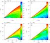Fig. 1 2D representations of the results obtained including isotope-selective effects for a representative model (Md = 10-2M⊙, T Tauri star, flarge = 10-2). The gas number density (panel a)), the dust temperature (panel b)), the FUV flux in units of G0 (panel c)), and the gas temperature (panel d)) are shown.

Reactions involving the rarer isotopologues are duplicates of those involving the dominant isotopologue. For example, the reaction H + O₂ → OH + O is expanded to the reactions

$\begin{array}{ccc}& & \mathrm{H}\mathrm{+}{}_{}^{\mathrm{16}}\mathrm{O}{}_{}^{\mathrm{18}}\mathrm{O}\mathrm{\to }{\hspace{0.17em}}^{\mathrm{16}}\mathrm{OH}\mathrm{+}{}_{}^{\mathrm{18}}\mathrm{O}\\ & & \mathrm{H}\mathrm{+}{}_{}^{\mathrm{16}}\mathrm{O}{}_{}^{\mathrm{18}}\mathrm{O}\mathrm{\to }{\hspace{0.17em}}^{\mathrm{18}}\mathrm{OH}\mathrm{+}{}_{}^{\mathrm{16}}\mathrm{O}\\ & & \mathrm{H}\mathrm{+}\begin{array}{c}\mathrm{18}\\ \end{array}\mathrm{O}2\mathrm{\to }{\hspace{0.17em}}^{\mathrm{18}}\mathrm{OH}\mathrm{+}{}_{}^{\mathrm{18}}\mathrm{O}\\ & & \mathrm{H}\mathrm{+}{}_{}^{\mathrm{16}}\mathrm{O}{}_{}^{\mathrm{17}}\mathrm{O}\mathrm{\to }{\hspace{0.17em}}^{\mathrm{16}}\mathrm{OH}\mathrm{+}{}_{}^{\mathrm{17}}\mathrm{O}\\ & & \mathrm{H}\mathrm{+}{}_{}^{\mathrm{16}}\mathrm{O}{}_{}^{\mathrm{17}}\mathrm{O}\mathrm{\to }{\hspace{0.17em}}^{\mathrm{17}}\mathrm{OH}\mathrm{+}{}_{}^{\mathrm{16}}\mathrm{O}\\ & & \mathrm{H}\mathrm{+}\begin{array}{c}\mathrm{17}\\ \end{array}\mathrm{O}2\mathrm{\to }{\hspace{0.17em}}^{\mathrm{17}}\mathrm{OH}\mathrm{+}{}_{}^{\mathrm{17}}\mathrm{O}\\ & & \mathrm{H}\mathrm{+}{}_{}^{\mathrm{18}}\mathrm{O}{}_{}^{\mathrm{17}}\mathrm{O}\mathrm{\to }{\hspace{0.17em}}^{\mathrm{18}}\mathrm{OH}\mathrm{+}{}_{}^{\mathrm{17}}\mathrm{O}\\ & & \mathrm{H}\mathrm{+}{}_{}^{\mathrm{18}}\mathrm{O}{}_{}^{\mathrm{17}}\mathrm{O}\mathrm{\to }{\hspace{0.17em}}^{\mathrm{17}}\mathrm{OH}\mathrm{+}{}_{}^{\mathrm{18}}\mathrm{O}\mathit{.}\end{array}$(4)

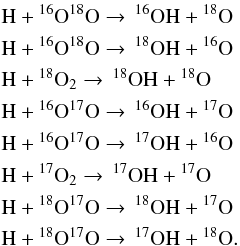
This procedure increases the number of reactions included in the network from 1463 to 9755. Since most of the rate coefficients for these reactions involving isotopologues are unknown, we follow the procedure by Röllig & Ossenkopf (2013) and assume that the isotopologue reactions with the same reactants, but different products, have the original reaction rate divided by the number of out-going channels. This implies assigning an equal probability to all branches.

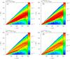Fig. 2 2D representations of the results obtained including isotope-selective effects for a representative model (Md = 10-2M⊙, T Tauri star, flarge = 10-2). The CO isotopologue abundances normalized to the total gas density are presented. The black solid line indicates the layer where the dust temperature is equal to 20 K. For lower Tdust values, CO freeze-out may become important.

The fractionation reactions (Eqs. (2) and (3)) were also added to the network. In addition to ¹³C, we also added the analogous reactions for ¹⁸O and ¹⁷O. When available, the reaction rate coefficients were taken from Röllig & Ossenkopf (2013), which are based on Langer et al. (1984). Coefficients for reactions with ¹⁷O are not provided, and extrapolations were made. For reaction (2), we used the same α and β for C¹⁷O as for ¹³CO and C¹⁸O (Sect. 2.1). The value of γ was obtained from scaling with the reduced mass of C¹⁷O following the procedure described in Langer et al. (1984). For reaction (3), the α and β coefficients were taken to be the same as that with ¹⁸O. For γ, we assumed the value to be the mean of the values for ¹⁶O and ¹⁸O, since the mass of ¹⁷O is the median of the ¹⁶O and ¹⁸O masses. For the conditions in protoplanetary disks, reaction (3) is less important for chemical fractionation than reaction (2); hence, this simple assumption is appropriate.

2.3. Parameters of the disk model

For our modeling, we assumed a simple parameterized density structure, similar to that reported by Andrews et al. (2011). Assuming a viscously evolving disk, where the viscosity ν = R^γ is a power law of the radius (Lynden-Bell & Pringle 1974; Hartmann et al. 1998), the surface density is given by ${\mathrm{\Sigma }}_{\mathrm{gas}}\mathrm{=}{\mathrm{\Sigma }}_{\mathrm{c}}\hspace{0.17em}{\left(\frac{\mathit{R}}{{\mathit{R}}_{\mathrm{c}}}\right)}^{\mathrm{-}\mathit{\gamma }}\exp \hspace{0.17em}\left[\mathrm{-}\hspace{0.17em}{\left(\frac{\mathit{R}}{{\mathit{R}}_{\mathrm{c}}}\right)}^{\mathrm{2}\mathrm{-}\mathit{\gamma }}\right]\mathit{,}$(5)with a characteristic radius R_c and a characteristic surface density Σ_c. The characteristic radius was fixed to R_c = 200 AU and the characteristic surface density Σ_c adjusted to yield a total disk mass M_gas with the outer radius fixed to R_out = 400 AU. The gas-to-dust ratio was assumed to be 100.

The vertical density structure follows a Gaussian with scale height angle h = h_c(R/R_c)^ψ. For the dust settling, two populations of grains were considered, small (0.005−1 μm) and large (1−1000 μm) (D’Alessio et al. 2006). The scale height is h for the the small and χh for the large grains, where χ< 1. The distribution of the surface density of the two species is given by the factor f_large as Σ_dust = f_large Σ_large + (1 − f_large)Σ_small.

Other parameters of the model are the stellar FUV (6−13.6 eV) and X-ray spectrum and the cosmic-ray ionization rate. To study the effects of different amounts of FUV photons compared with the bolometric luminosity, the stellar spectrum was assumed to be a black body at a given temperature T_eff. The strength of the FUV field in units of the interstellar radiation field G₀ is given in Fig. 1 for a representative model. Here, G₀ = 1 refers to the interstellar radiation field defined as in Draine (1978)~ 2.7 × 10^-3 erg s^-1 cm^-2 with photon-energies E_γ between 6 eV and 13.6 eV. The X-ray spectrum was taken to be a thermal spectrum of 7 × 10⁷ K within 1–100 keV and the X-ray luminosity in this band L_X = 10³⁰ erg s^-1. As discussed in Bruderer (2013), the X-ray luminosity is of minor importance for the intensity of CO pure rotational lines that are the focus in this work. The cosmic-ray ionization rate was set to 5 × 10^-17 s^-1. We accounted for the interstellar UV radiation field and the cosmic microwave background as external sources of radiation.

The calculation was carried out on 75 cells in the radial direction and 60 in the vertical directions. In the radial direction the spatial grid is on a logarithmic scale up to 30 AU (35 cells) and on a linear scale from 30 AU to 400 AU (40 cells). The spectral grid of the continuum radiative transfer extends from 912 Å to 3 mm in 58 wavelength-bins. The wavelength dependence of the cross section wass taken into account using data summarized in van Dishoeck et al. (2006).

The chemistry was solved in a time dependent manner, up to a chemical age of 1 Myr. The main difference to the steady-state solution is that carbon is not converted into methane (CH₄) close to the mid-plane, since the time-scale of these reactions is longer than >10 Myr and thus is unlikely to proceed in disks. We ran models both with isotopologues and isotope-selective processes switched on (network ISO) or off (network NOISO).

2.4. Grid of models

The goal of our work is to understand the effect of isotope-selective processes in disks and to quantify their importance when rare isotopologue observations are used to measure the total gas mass. We ran a small grid of models to explore some of the key parameters.

• 1.

  Stellar spectrum. The first parameter to explore is the fraction ofFUV photons (912−2067 Å) over the entire stellar spectrum. A spectrum with T_eff = 4000 K and T_eff = 10 000 K was considered, to simulate a T Tauri or Herbig Ae star. Accordingly, we ran models with a bolometric luminosity of L_bol = 1 or 10 L_⊙. Excess UV radiation due to accretion was taken into account for T Tauri stars. It was assumed that the gravitational potential energy of accreted mass is released with 100% efficiency as blackbody emission with T = 10 000 K. The mass accretion rate was taken to be 10^-8M_⊙ yr^-1 and the luminosity was assumed to be emitted uniformly over the stellar surface. These assumptions result in L_FUV/L_bol = 1.5 × 10^-2 for the T Tauri case versus L_FUV/L_bol = 7.8 × 10^-2 for the Herbig case. The ratio of CO photodissociating photons (912−1100 Å) between the T Tauri and the Herbig cases is F_CO,pd(T Tau)/F_CO,pd(Her) = 2.5 × 10^-2. In all models, the interstellar UV field was included as well.

• 2.

  Dust properties. Since small grains are much more efficient in absorbing UV radiation, the ratio of large to small grains was varied. We considered f_large = 0.99 in order to simulate a mixture of the two populations and f_large = 10^-2 for the situation where only small grains are present in the disk (no or little grain growth).

• 3.

  Disk mass. Three different values for the total disk mass M_d were considered to cover a realistic range of disks (M_gas = 10^-2,10^-3,10^-4M_⊙).

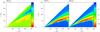Fig. 3 CO isotopologue abundance ratios obtained using the NOISO and the ISO chemical networks. The ratios are defined as follows: ${\mathit{Rat}}_{\mathrm{13}}^{\mathit{n}}\mathrm{=}\mathrm{77}\mathrm{·}\frac{\mathit{n}\mathrm{(}{\mathrm{13}}_{}^{}\mathrm{CO}{\mathrm{)}}_{\mathrm{ISO}}}{\mathit{n}\mathrm{(}\mathrm{CO}{\mathrm{)}}_{\mathrm{NOISO}}}$, ${\mathit{Rat}}_{\mathrm{18}}^{\mathit{n}}\mathrm{=}\mathrm{560}\mathrm{·}\frac{\mathit{n}\mathrm{(}{\mathrm{C}}_{\mathrm{18}}^{}\mathrm{O}{\mathrm{)}}_{\mathrm{ISO}}}{\mathit{n}\mathrm{(}\mathrm{CO}{\mathrm{)}}_{\mathrm{NOISO}}}$ and ${\mathit{Rat}}_{\mathrm{17}}^{\mathit{n}}\mathrm{=}\mathrm{1792}\mathrm{·}\frac{\mathit{n}\mathrm{(}{\mathrm{C}}_{\mathrm{17}}^{}\mathrm{O}{\mathrm{)}}_{\mathrm{ISO}}}{\mathit{n}\mathrm{(}\mathrm{CO}{\mathrm{)}}_{\mathrm{NOISO}}}$. The plots show the results for a 10-2M⊙ disk around a T Tauri star, with flarge = 10-2.

3. Results

3.1. Abundances

In Fig. 2 we present the abundances of CO and its isotopologues computed using the ISO network and implementing the isotopologue shielding factors in a representative model. (T Tauri star, M_disk = 10^-2M_⊙, f_large = 10^-2.) In panel (a) a 2D distribution of ${\mathrm{12}}_{}^{}\mathrm{CO}$ in a disk quadrant is shown; the central star is located at the origin of the axis. As the disk surface is directly illuminated by the FUV stellar and interstellar radiation, CO is easily photodissociated and its abundance drops, such that n(CO) /n_gas reaches values around 10^-8. This so-called photodissociation layer results in a low-abundance region shown in green in panel (a) of Fig. 2. The depth of this layer is not radially constant because it depends on the disk surface density structure and on the FUV flux. At large radii both H₂ and CO column densities are lower and the FUV stellar flux is less strong: CO is not shielded until lower heights compared with regions at smaller radii. As soon as the UV absorption lines saturate because of (self-) shielding, the photodissociation rate decreases steeply, allowing CO to survive in the interior of the disk. This warm, high-abundance layer of survived CO is shown in red in panel (a) of Fig. 2. It extends from the surface up to the midplane at very small radii, R< 40 AU, because the column densities there are high enough that CO can survive the strong stellar photodissociating flux, and the dust grains are warm enough to prevent freeze-out. At radii larger than 40 AU, the abundance of CO falls again at decreasing height toward the midplane. There the dust temperature is very low (T_dust ≲ 20 K) because the UV stellar flux is well shielded by the higher regions. At such temperatures CO molecules freeze out onto dust grains, therefore the abundance of gaseous CO decreases. The precise dust temperature at which most of the CO is frozen out depends on the density and can be as low as 18 K for the adopted CO binding energy.

The shape of the distribution of C¹⁸O and C¹⁷O inside the disk appears different from that of CO (panels (c) and (d), Fig. 2), while the distribution of ${\mathrm{13}}_{}^{}\mathrm{CO}$ is similar to that of CO (panel (b), Fig. 2). For the two less abundant isotopologues the warm molecular layer is indeed much thinner and separated by a warm molecular finger at the midplane at small radii, R< 200 AU. This difference in the molecular distribution is the effect of the isotope selective photodissociation and is highlighted in Fig. 3 through the abundance ratios: $\mathit{Ra}{\mathit{t}}_{\mathit{xy}}^{\mathit{n}}\mathrm{=}\frac{\mathit{n}\mathrm{\left(}{\mathit{x}}_{}^{}\mathrm{C}{\mathit{y}}_{}^{}\mathrm{O}\mathrm{\right)}[{\mathrm{12}}_{}^{}\mathrm{C}][{\mathrm{16}}_{}^{}\mathrm{O}]}{\mathit{n}\left({\mathrm{12}}_{}^{}\mathrm{CO}\right)\mathrm{\left[}{\mathit{x}}_{}^{}\mathrm{C}\mathrm{\right]}\mathrm{\left[}{\mathit{y}}_{}^{}\mathrm{O}\mathrm{\right]}}\mathrm{·}$(6)This indicates that the conventional way of deriving the CO isotopologue abundances by simply dividing the ${\mathrm{12}}_{}^{}\mathrm{CO}$ abundance by the isotope ratios is not accurate.

In Fig. 3 the ratios of the abundances found using these two methods are presented, that is, the differences in the predictions whether or not the isotope-selective processes are taken into account. In the right-hand panels, the regions where C¹⁸O and C¹⁷O are not yet self-shielded, while ¹²CO is, blow-up clearly. In these regions the isotopologue ratios are lower by up to a factor of 40 compared with just rescaling the isotope ratios.These isotope-selective effects for the ¹⁸O and ¹⁷O species are also clearly seen when the values of $\mathit{Ra}{\mathit{t}}_{\mathit{xy}}^{\mathit{n}}$ for the total number of CO molecules summed over the whole disk are compared in Table 2.

Another way to present the isotopologue fractionation is through ℛ, the cumulative column density ratios normalized to ¹²CO and the isotopic ratios reported, as by Visser et al. (2009), for instance $\mathrm{ℛ}\mathrm{\left(}\mathit{z}\mathrm{\right)}\mathrm{=}\frac{{\mathit{N}}_{\mathit{z}}\mathrm{\left(}{\mathit{x}}_{}^{}\mathrm{C}{\mathit{y}}_{}^{}\mathrm{O}\mathrm{\right)}[{\mathrm{12}}_{}^{}\mathrm{C}][{\mathrm{16}}_{}^{}\mathrm{O}]}{{\mathit{N}}_{\mathit{z}}\left({\mathrm{12}}_{}^{}\mathrm{CO}\right)[{\mathit{x}}_{}^{}\mathrm{C}][{\mathit{y}}_{}^{}\mathrm{O}]}\mathit{,}$(7)where [X] is the elemental abundance of isotope X and ${\mathit{N}}_{\mathit{z}}\mathrm{\left(}{\mathit{x}}_{}^{}\mathrm{C}{\mathit{y}}_{}^{}\mathrm{O}\mathrm{\right)}\mathrm{\left(}\mathit{z}\mathrm{\right)}\mathrm{=}\underset{\mathit{z}}{\overset{{\mathit{z}}_{\mathrm{surf}}}{\mathrm{\int }}}\mathit{n}\mathrm{\left(}{\mathit{x}}_{}^{}\mathrm{C}{\mathit{y}}_{}^{}\mathrm{O}\mathrm{\right)}\hspace{0.17em}\mathrm{d}{\mathit{z}}^{\mathrm{\prime }}\mathit{,}$(8)is the column density, integrated from the surface of the disk (z_surf) down to the height z.

Figure 4 shows ℛ as function of disk height through a vertical cut at a radius of 150 AU for the three isotopologues in two representative models. Consistent with Visser et al. (2009), for C¹⁸O and C¹⁷Oℛ is found to be constant around unity, until it dips strongly at intermediate heights. There ℛ perceptibly drops because ¹²CO is already self-shielded and survives the photodissociation, while UV photons still dissociate C¹⁸O and C¹⁷O. This is the region where isotope-selective effects are most detectable. If only small grains are present in the disk (upper panel of Fig. 4), the temperature at which CO can freeze out (T_dust ≲ 20 K) is reached below z = 10 AU, where the cumulative ratios are back close to the elemental isotope ratios (ℛ ~ 1). On the other hand, if large grains are considered (lower panel), this threshold shifts to 25 AU, just in the region where isotope-selective dissociation is most efficient. For heights lower than 25 AU the tiny amount of C¹⁸O and C¹⁷O remaining in the gas phase does not add to the column density, so ℛ is effectively frozen at around 0.2 for both isotopologues. ¹³CO, on the other hand, has less fractionation in both models. ℛ, however, increases by a factor of three at intermediate heights (around z = 40 AU) for this isotopologue as a result of gas-phase reactions. For each isotopologue, isotope-selective effects are maximized if mm-sized grains are present in the disk, as we discuss in Sect. 3.2 in more detail.

A negligible fraction of CO is in solid CO in our models, in particular for the warm Herbig disks. Only the more massive cold disks around T Tauri stars have a solid CO fraction similar to that of gaseous CO. Overall, a large portion of oxygen is locked up in water ice in the models. In particular, the excess ¹⁸O and ¹⁷O produced by the isotope-selective photodissociation is turned into water ice, which has a much higher binding energy and thus remains on the grains even in warm disks. If this water ice subsequently comes into contact with solids that drift inwards, this may explain the anomalous ¹⁸O and ¹⁷O isotope ratios found in meteorites (Lyons & Young 2005; Visser et al. 2009).

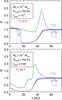Fig. 4 Cumulative column density ratios normalized to 12CO and the isotopic ratios (see Eq. (7)) shown as a function of height for a vertical cut through the disk at a radius of 150 AU. In the top panel we show a 10-3M⊙ disk around a T Tauri star with f = 10-2 (only small grains), while in the bottom panel the settling parameter is flarge = 0.99. The dotted red lines indicate where the temperature reaches 20 K, below which CO starts to freeze out.

3.2. Line fluxes

While the 2D representations of molecular abundances shown in Figs. 2 and 3 are useful for understanding the chemical and physical structures of the disk, line fluxes are a better proxy for quantifying the observable effects given by the isotope-selective processes. In Fig. 6 we present the radial intensity ratios of the J = 3−2 line for ¹³CO,C¹⁸O, and C¹⁷O obtained with the NOISO and ISO networks. Spectral-image cubes were obtained with DALI from the solution of the radiative transfer equation, assuming the disk is at a distance of 100 pc. The derived line intensities were not convolved with any observational beam. For ¹³CO the line intensities obtained with the two networks are very similar, leading to line ratios within a factor of two. On the other hand, for C¹⁸O and C¹⁷O the line intensity ratios obtained with the two networks differ by up to a factor of 40. This means that an analysis that does not consider isotope-selective effects would lead to an overprediction of the line intensity of the two less abundant isotopologues at radii around 100 AU. Using the NOISO network would overpredict the C¹⁸O and C¹⁷O lines intensities by up to a factor of 40.

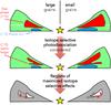Fig. 5 Sketch of the 2D abundances of C18O in one quadrant of the disk. On the left-hand side mm-sized grains are present in the disk (flarge = 0.99), while on the right just (sub) μm-sized grains are considered (flarge = 10-2). In the upper panel the 2D abundance predicted by the NOISO network (i.e., not considering isotope selective photodissociation) is plotted, in the middle panel that inferred by the ISO network, i.e., with an isotopologue selective treatment of isotopologues. The red regions show where CO isotopologues are in the molecular phase, while the blue regions are where they are frozen onto grains. The regions where the two predictions differ more are those in which isotope-selective processes are strongest; they are highlighted in the lower panel by the white shapes. The black dotted contours and the red arrows show the difference between ISO and NOISO. Since small grains are more efficient in shielding from photodissociating photons, C18O can survive in the gas phase at grater heights and farther out (white dotted lines in the upper panel). Accordingly, the white regions that show the difference between ISO and NOISO in the lower panel also shift upward and outward in the case of small grains.

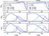Fig. 6 Ratios of CO isotopologue line intensity (J = 3−2) obtained with the NOISO and ISO networks as a function of the disk radius. ${\mathit{Rat}}_{\mathrm{13}}^{\mathrm{I}}\mathrm{=}\mathit{I}{\mathrm{[}}^{\mathrm{13}}\mathrm{CO}{\mathrm{]}}_{\mathrm{NOISO}}$/I [ 13CO ] ISO, ${\mathit{Rat}}_{\mathrm{18}}^{\mathrm{I}}\mathrm{=}\mathit{I}\mathrm{[}{\mathrm{C}}^{\mathrm{18}}\mathrm{O}{\mathrm{]}}_{\mathrm{NOISO}}$/I [ C18O ] ISO and ${\mathit{Rat}}_{\mathrm{17}}^{\mathrm{I}}\mathrm{=}\mathit{I}\mathrm{[}{\mathrm{C}}^{\mathrm{17}}\mathrm{O}{\mathrm{]}}_{\mathrm{NOISO}}$/I [ C17O ] ISO were defined. Dotted lines refer to models where f = 10-2, solid lines to flarge = 0.99. Different colors indicate models with different disk masses: Md = 10-4M⊙ in blue, Md = 10-3M⊙ in light blue and Md = 10-2M⊙ in purple. Models with T Tauri stars are shown in the left panels, those with Herbig stars in the right panels.

3.2.1. Dependence on the parameters

It is interesting to determine how the observables depend on the variation of the parameters listed in Sect. 2.4. The focus is in particular on the line intensity ratios found for C¹⁸O and C¹⁷O, where the effects are more prominent.

When the dust composition is left unchanged and the disk mass is increased from M_d = 10^-4M_⊙ to M_d = 10^-2M_⊙, the region where the isotope-selective photodissociation is most effective shifts toward the outer regions. The peak of the intensity ratios between the ISO and NOISO networks is located there (second and third panels of Fig. 6). They are defined as ${\mathit{Rat}}_{\mathrm{13}}^{\mathrm{I}}\mathrm{=}\mathit{I}{\mathrm{[}}^{\mathrm{13}}\mathrm{CO}{\mathrm{]}}_{\mathrm{NOISO}}\mathit{/}$I [ ¹³CO ] _ISO, ${\mathit{Rat}}_{\mathrm{18}}^{\mathrm{I}}\mathrm{=}\mathit{I}\mathrm{[}{\mathrm{C}}^{\mathrm{18}}\mathrm{O}{\mathrm{]}}_{\mathrm{NOISO}}\mathit{/}$I [ C¹⁸O ] _ISO and ${\mathit{Rat}}_{\mathrm{17}}^{\mathrm{I}}\mathrm{=}\mathit{I}\mathrm{[}{\mathrm{C}}^{\mathrm{17}}\mathrm{O}{\mathrm{]}}_{\mathrm{NOISO}}\mathit{/}$I [ C¹⁷O ] _ISO. At higher masses the column densities at which CO UV-lines saturate are reached earlier: CO and its isotopologues can therefore survive at larger radii and heights and the observable effects of isotope-selective photodissociation come from the outer regions. Higher mass disks also have colder deeper regions and thus more CO freeze-out onto dust grains in the midplane.

A similar and even more substantial shift toward larger radii is seen by considering two models with the same disk mass, but with different dust composition. Submicron-sized particles are much more efficient than mm-sized grains in shielding FUV phodissociating photons, therefore the observable effects of isotope-selective photodissociations come from outer regions. This behavior is sketched in Fig. 5 where it is shown that the CO emitting region shifts deeper into the disk and inward with grain growth, as found previously by Jonkheid et al. (2004) and Aikawa & Nomura (2006).

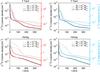Fig. 7 Column density radial profiles of C18O and C17O compared with beam-convolved line intensity (J = 3−2) radial profiles. Different line styles represent models with various disk masses; column densities in black, C18O and C17O line intensities in red and in blue, convolved with a 0.1′′ beam. Models with a central T Tauri star are presented in the left panels, those with a Herbig star in the right panels. Only models with flarge = 0.99 are shown.

The magnitude of the isotope-selective effects is lower in the case of small grains, however. The peak in line intensity ratios is a factor of 2 lower than for large grains. The explanation is in the location of the freeze out zone. For large grains the region where less abundant CO isotopologues are highly fractionated partially coincides with the freeze-out zone (see Fig. 4). For T_dust ≲ 20 K almost all CO molecules are frozen onto grains, except for a small fraction that is photodesorbed by FUV radiation, and the tiny fraction that remains in the gas phase cannot substantially enhance the line intensity.

The last parameter to consider is the spectrum of the central star. In Fig. 6 the line intensity ratios obtained considering a T Tauri star and a Herbig star are presented. There is no substantial difference in the peak values of the ratios, but their location depends on the stellar spectrum. For low-mass disks the peak for both T Tauri and Herbig disks is in the inner region, while for high-mass disks the Herbig emission peaks at larger radii. For example, for the model with the highest mass, M_d = 10^-2M_⊙, and with large grains, f_large = 0.99, the peak shifts drastically outward at ≈200 AU for a Herbig star. This shift is caused by the fact that Herbig stars have more CO-dissociating UV photons (λ< 1100 Å), than T Tauri stars.

3.3. Line optical depth

C¹⁸O is frequently used as a mass tracer because of its low abundance. Compared with more abundant isotopologues such as ¹²CO and ¹³CO, its detection allows probing regions closer to the midplane and thus the bulk of the disk mass. C¹⁸O is a good mass tracer as long as its lines are optically thin, which may not always be the case. Then C¹⁷O, being rarer than C¹⁸O, can be used to probe the regions where the optical depth is greater than unity.

One way to investigate line optical thickness is to compare the line intensity radial profile with the column density radial profile. For optically thin emission, they should indeed follow the same trend, since column density counts the total number of molecules at a given column. If the line intensity radial profile does not follow that of the column density, this is a signature of an opacity effect.

In Fig. 7 column density radial profiles are compared with line intensity radial profiles for models with a T Tauri star and with a Herbig star as central objects. Column densities are shown in black, while line intensities are shown in red for C¹⁸O and in light blue for C¹⁷O. Except for the very inner and dense regions, both isotopologues are optically thin throughout the entire disk. This is true in particular for the 10^-4M_⊙ disks, but not completely for the massive 10^-2M_⊙ T Tauri disk.

It is interesting to note that in Fig. 7 in the outer regions, that is for r> 200 AU, the column densities obtained with different models do not scale linearly with mass. This depends on the amount of C¹⁸O and C¹⁷O frozen onto grains, which varies for the different models. In Fig. 8 the C¹⁸O and the total (H + 2H₂) cumulative column densities (Eq. (8)) are shown for a cut at r = 300 AU. The total cumulative column densities are divided by a factor 10^-9. For z = 0, that is where the column densities are integrated from the surface up to the midplane, the total cumulative column density scales linearly with mass as expected, but that of C¹⁸O does not, because of the different freeze-out zones.

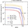Fig. 8 Cumulative column density as a function of the disk height integrating from the surface to the midplane in a disk radial cut (r = 300 AU). Only T Tauri models with flarge = 0.99 are shown. Different line colors represent models with various disk masses. Dotted lines show the scaled total gas cumulative column density (see text), solid lines that of C18O. The black lines show where the dust temperature is lower than 20 K for the different disk models, i.e., where CO freeze-out becomes important.

4. Discussion

To properly compare model predictions with data, one needs to convolve output images with the same beam as used for observations. Whether or not the isotope-selective effects presented in previous sections can indeed be detected may vary with different beam sizes. Moreover, estimates of the total disk masses may be affected by this choice. Below we discuss this problem and provide estimates of the magnitude of this effect in determining disk masses.

4.1. Beam convolutions

To investigate the sensitivities of mass estimates on isotope selective effects, the output images obtained by implementing the ISO and NOISO network were convolved with different observationals beams. Four beam sizes were adopted for the convolution: 0.1′′, 0.5′′, 1.0′′, and 3.0′′. The smallest are useful to simulate high-resolution observations (e.g., ALMA observations), while the largest are used to compare the models with lower resolution observations (e.g., Submillimeter Array, SMA, observations) or disk-integrated (single-dish) measurements.

In Fig. 9 radial distributions of C¹⁸O line intensity obtained with different beam convolutions are presented for one of the T Tauri disk models located at 100 pc. Different colors refer to various beam sizes, while the line style shows whether isotope-selective effects are taken into account or not: a solid line is used if they are considered (ISO network), a dotted line otherwise (NOISO network). The predictions obtained with the two chemical networks always differ, but they do so in diverse ways if different beam sizes are adopted. In the extreme case of the 3′′ beam, the NOISO network overproduces the disk-integrated C¹⁸O line intensity by a factor of 5. On the other hand, if a very narrow beam is used for the convolution, that is, a 0.1′′ beam, the line intensities are the same at very small radii for the two models; but at larger distances the NOISO network overestimates the line intensity, but not always by the same factor. Such a narrow beam allows resolving substructures that are smeared out by a larger beam. As expected, the regions of the disk where line intensity ratios of ISO and NOISO are high are the same as those for which the unconvolved line intensities obtained with the two networks differ most (see Fig. 6).

4.2. Mass estimates

The question to answer now is how much disk mass estimates may vary if a proper treatment of CO isotopologues is adopted. Unfortunately, ¹³CO, the isotopologue less affected by isotopologue selective processes, becomes optically thick at substantial heights from the midplane, and is thus not a good mass tracer (Fig. 10, top). Therefore just C¹⁸O and C¹⁷O can be considered for mass estimates.

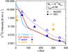Fig. 9 Radial profiles of the C18O line intensity (J = 3−2) considering different observational beams for a particular disk model (T Tauri star, Mdisk = 10-3M⊙,fsmall = 0.99). Different colors show different choices of the observational beam size. Solid lines represent the intensities obtained considering the isotope-selective processes (ISO network), dotted lines show the results when an approximative analysis is carried out (NOISO network). For the 0.1′′ and 0.5′′ beam, full lines are presented, whereas for the 1′′ and 3′′ beam they are binned at the spatial resolution. For the 3′′ beam, only the disk-integrated value (or the value that just resolves the outer disk) is shown.

For spatially resolved observations (0.1′′−1′′), the difference between the line intensities obtained with the NOISO and ISO networks varies through the disk (see Fig. 9). This is because isotope selective processes have different influence in different regions of the disk. Therefore, as our analysis concluded, no simple scaling relation can be given, but a full thermochemical model needs to be run to estimate the correct disk mass.

On the other hand, in the extreme case of a 3′′ observational beam, where the disk substructures are not resolved, the bulk of the disk-integrated line intensity is obtained. In Fig. 10 the integrated line intensities obtained with disk masses M_d = 10^-4,10^-3 and 10^-2M_⊙ are shown, for the NOISO and the ISO network. The red line relates the intensity values obtained for the three disk masses with the NOISO network, while the blue line shows those with the ISO network. The dotted lines indicate the different masses inferred by the two networks, and thus the factor by which the total disk mass is underestimated if isotope-selective processes are neglected. Both grain growth level and variation in the stellar spectrum are investigated. The inferred masses, both considering isotope selective processes and not considering them, are presented in Table 3, together with their ratios. In practice, a given C¹⁸O and C¹⁷O line intensity is observed and plots such as those in Fig. 10 can then be used to draw a horizontal line and read off the disk masses.

The grid of models presented in this paper explores only a few parameters, and it is not possible to draw a general correction rule; we stress that the values in Table 3 are only indicative and may well reproduce extreme cases. On the other hand, it is possible to find trends in the results. For a given C¹⁸O or C¹⁷O intensity, the total disk mass is always underestimated if the NOISO network is used, that is, if isotope-selective effects are not properly considered. The underestimates are higher if mm-sized grains are present in the disk (i.e., where photodissociation is most efficient) and for a T Tauri star as central object, whose disk is cold. Moreover, the results differ by a larger factor if more massive disks are considered, such as disks with masses that range from 10^-3M_⊙ to 10^-2M_⊙.

Williams & Best (2014) used a simple parametric approach to infer disk masses from their ¹³CO and C¹⁸O data assuming constant isotopologue abundance ratios in those regions of the disk where CO is not photodissociated or frozen out. Effects of isotope selective photodissociation are treated by decreasing the C¹⁸O/CO abundance ratio by an additional constant factor of 3 throughout the disk. Although our mini-grid is much smaller than that of Williams & Best (2014), we tend to find higher ¹³CO and lower C¹⁸O intensities by up to a factor of a few for the same disk mass, especially for the models with large grains at the low mass end. A more complete parameter study of our full chemical models is needed for proper comparison.

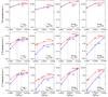Fig. 10 Disk-integrated 13CO (top), C18O (middle), and C17O (bottom) line intensities (J = 3−2) obtained with disk masses Md = 10-4,10-3,10-2M⊙ are shown as a function of the disk mass. The beam size is 3′′. The red line relates the intensity values obtained for the three disk masses with the NOISO network, while the blue line shows those with the ISO network. Dotted lines indicate by which factor the total disk mass is underestimated if no isotope-selective processes are considered. Results are presented for flarge = 10-2, 0.99 and for T Tauri and Herbig disks.

4.3. TW Hya

TW Hya is one of the best-studied protoplanetary disks, being the closest T Tauri system, at a distance of 54 ± 6 pc from Earth (van Leeuwen 2007). In addition, it is the only case in which the fundamental rotational transition of HD has been detected with the Herschel Space Observatory (Bergin et al. 2013). Observations of HD emission lines provide an independent disk mass determination, assuming that the HD distribution follows that of H₂. From these observations Bergin et al. (2013) determined a total disk mass larger than 5 × 10^-2M_⊙. Favre et al. (2013) also reported spatial integrated C¹⁸O (2−1) observations of TW Hya with SMA. From their analysis an underestimate of the disk mass by a factor between 3 and 100 was found. In their modeling they did not treat isotope selective photodissociation in a self-consistent way and concluded instead that the carbon abundance is low.

For the model in our grid that best represents the TW Hya characteristics (T Tauri star, large grains, M_d = 10^-2M_⊙), a mass correction factor of at least 20 is found (see Table 3). This demonstrates that accounting for isotope selective processes might mitigate the disagreement in mass determinations. The spatial resolution of the SMA data of 100–150 AU is just in the regime where the effects are strongest. A more accurate modeling of TW Hya implementing the full isotope selective photodissociation using the same disk model as in Favre et al. (2013), Bergin et al. (2013) and Cleeves et al. (2014) with the observed stellar UV spectrum is needed to support this claim.

5. Summary and conclusions

We presented a detailed treatment of CO isotope selective photodissociation in a complete disk model for the first time. A full thermo-chemical model was used to which less abundant CO isotopologues were added into the chemical network as independent species, and the corresponding self-shielding factors were implemented. Abundances and line intensities were obtained as outputs for a grid of disk models, with and without isotope-selective photodissociation. The main conclusions are listed below.

• When CO isotope selective photodissociation is considered, the abundances of CO isotopologues are affected. In particular, there are regions in the disk where C¹⁸O and C¹⁷O show an underabundance with the respect to ¹²CO when compared with the overall elemental abundance ratios.

• The CO isotopologue line intensity ratios vary if isotope selective photodissociation is properly considered. The line intensity ratios are overestimated by up to a factor of 40 at certain disk radii, when isotope selective processes are not included into the modeling.

• A consequence of these results is that the disk mass can be underestimated by up to almost two orders of magnitude if a single line is observed and isotope selective effects are not properly taken into account. The effects are strongest for cold disks with large grains where the isotope selective effects are strongest close to the freeze-out zone, i.e., the same region of the disk from which most of the C¹⁸O and C¹⁷O emission arises. Moreover, the situation is worse for single-dish data or for low spatial resolution interferometry, which just resolves the outer disk.

• A preliminary comparison was made between the results presented here and TW Hya. The discrepancy in mass determination observed for this object may be explained by implementing isotope selective photodissociation in a self-consistent manner. More detailed modeling of the object is still needed, however.

In the future we will model TW Hya and other disks in more detail. In addition, a wider set of parameters will be explored in a larger grid of models, to provide mass estimate corrections for all kinds of disks when multiple lines are observed.

Online material

Appendix A: Appendix A

Acknowledgments

The authors are grateful to Ruud Visser, Ilsedore Cleeves, Catherine Walsh, Mihel Kama, and Leonardo Testi for useful discussions and comments. Astrochemistry in Leiden is supported by the Netherlands Research School for Astronomy (NOVA), by a Royal Netherlands Academy of Arts and Sciences (KNAW) professor prize, and by the European Union A-ERC grant 291141 CHEMPLAN.

References

All Tables

All Figures

	Fig. 1 2D representations of the results obtained including isotope-selective effects for a representative model (Md = 10-2M⊙, T Tauri star, flarge = 10-2). The gas number density (panel a)), the dust temperature (panel b)), the FUV flux in units of G0 (panel c)), and the gas temperature (panel d)) are shown.
In the text

	Fig. 2 2D representations of the results obtained including isotope-selective effects for a representative model (Md = 10-2M⊙, T Tauri star, flarge = 10-2). The CO isotopologue abundances normalized to the total gas density are presented. The black solid line indicates the layer where the dust temperature is equal to 20 K. For lower Tdust values, CO freeze-out may become important.
In the text

Fig. 3 CO isotopologue abundance ratios obtained using the NOISO and the ISO chemical networks. The ratios are defined as follows: ${\mathit{Rat}}_{\mathrm{13}}^{\mathit{n}}\mathrm{=}\mathrm{77}\mathrm{·}\frac{\mathit{n}\mathrm{(}{\mathrm{13}}_{}^{}\mathrm{CO}{\mathrm{)}}_{\mathrm{ISO}}}{\mathit{n}\mathrm{(}\mathrm{CO}{\mathrm{)}}_{\mathrm{NOISO}}}$, ${\mathit{Rat}}_{\mathrm{18}}^{\mathit{n}}\mathrm{=}\mathrm{560}\mathrm{·}\frac{\mathit{n}\mathrm{(}{\mathrm{C}}_{\mathrm{18}}^{}\mathrm{O}{\mathrm{)}}_{\mathrm{ISO}}}{\mathit{n}\mathrm{(}\mathrm{CO}{\mathrm{)}}_{\mathrm{NOISO}}}$ and ${\mathit{Rat}}_{\mathrm{17}}^{\mathit{n}}\mathrm{=}\mathrm{1792}\mathrm{·}\frac{\mathit{n}\mathrm{(}{\mathrm{C}}_{\mathrm{17}}^{}\mathrm{O}{\mathrm{)}}_{\mathrm{ISO}}}{\mathit{n}\mathrm{(}\mathrm{CO}{\mathrm{)}}_{\mathrm{NOISO}}}$. The plots show the results for a 10-2M⊙ disk around a T Tauri star, with flarge = 10-2.

In the text

Fig. 4 Cumulative column density ratios normalized to 12CO and the isotopic ratios (see Eq. (7)) shown as a function of height for a vertical cut through the disk at a radius of 150 AU. In the top panel we show a 10-3M⊙ disk around a T Tauri star with f = 10-2 (only small grains), while in the bottom panel the settling parameter is flarge = 0.99. The dotted red lines indicate where the temperature reaches 20 K, below which CO starts to freeze out.

In the text

Fig. 5 Sketch of the 2D abundances of C18O in one quadrant of the disk. On the left-hand side mm-sized grains are present in the disk (flarge = 0.99), while on the right just (sub) μm-sized grains are considered (flarge = 10-2). In the upper panel the 2D abundance predicted by the NOISO network (i.e., not considering isotope selective photodissociation) is plotted, in the middle panel that inferred by the ISO network, i.e., with an isotopologue selective treatment of isotopologues. The red regions show where CO isotopologues are in the molecular phase, while the blue regions are where they are frozen onto grains. The regions where the two predictions differ more are those in which isotope-selective processes are strongest; they are highlighted in the lower panel by the white shapes. The black dotted contours and the red arrows show the difference between ISO and NOISO. Since small grains are more efficient in shielding from photodissociating photons, C18O can survive in the gas phase at grater heights and farther out (white dotted lines in the upper panel). Accordingly, the white regions that show the difference between ISO and NOISO in the lower panel also shift upward and outward in the case of small grains.

In the text

Fig. 6 Ratios of CO isotopologue line intensity (J = 3−2) obtained with the NOISO and ISO networks as a function of the disk radius. ${\mathit{Rat}}_{\mathrm{13}}^{\mathrm{I}}\mathrm{=}\mathit{I}{\mathrm{[}}^{\mathrm{13}}\mathrm{CO}{\mathrm{]}}_{\mathrm{NOISO}}$/I [ 13CO ] ISO, ${\mathit{Rat}}_{\mathrm{18}}^{\mathrm{I}}\mathrm{=}\mathit{I}\mathrm{[}{\mathrm{C}}^{\mathrm{18}}\mathrm{O}{\mathrm{]}}_{\mathrm{NOISO}}$/I [ C18O ] ISO and ${\mathit{Rat}}_{\mathrm{17}}^{\mathrm{I}}\mathrm{=}\mathit{I}\mathrm{[}{\mathrm{C}}^{\mathrm{17}}\mathrm{O}{\mathrm{]}}_{\mathrm{NOISO}}$/I [ C17O ] ISO were defined. Dotted lines refer to models where f = 10-2, solid lines to flarge = 0.99. Different colors indicate models with different disk masses: Md = 10-4M⊙ in blue, Md = 10-3M⊙ in light blue and Md = 10-2M⊙ in purple. Models with T Tauri stars are shown in the left panels, those with Herbig stars in the right panels.

In the text

Fig. 7 Column density radial profiles of C18O and C17O compared with beam-convolved line intensity (J = 3−2) radial profiles. Different line styles represent models with various disk masses; column densities in black, C18O and C17O line intensities in red and in blue, convolved with a 0.1′′ beam. Models with a central T Tauri star are presented in the left panels, those with a Herbig star in the right panels. Only models with flarge = 0.99 are shown.

In the text

Fig. 8 Cumulative column density as a function of the disk height integrating from the surface to the midplane in a disk radial cut (r = 300 AU). Only T Tauri models with flarge = 0.99 are shown. Different line colors represent models with various disk masses. Dotted lines show the scaled total gas cumulative column density (see text), solid lines that of C18O. The black lines show where the dust temperature is lower than 20 K for the different disk models, i.e., where CO freeze-out becomes important.

In the text

Fig. 9 Radial profiles of the C18O line intensity (J = 3−2) considering different observational beams for a particular disk model (T Tauri star, Mdisk = 10-3M⊙,fsmall = 0.99). Different colors show different choices of the observational beam size. Solid lines represent the intensities obtained considering the isotope-selective processes (ISO network), dotted lines show the results when an approximative analysis is carried out (NOISO network). For the 0.1′′ and 0.5′′ beam, full lines are presented, whereas for the 1′′ and 3′′ beam they are binned at the spatial resolution. For the 3′′ beam, only the disk-integrated value (or the value that just resolves the outer disk) is shown.

In the text

Fig. 10 Disk-integrated 13CO (top), C18O (middle), and C17O (bottom) line intensities (J = 3−2) obtained with disk masses Md = 10-4,10-3,10-2M⊙ are shown as a function of the disk mass. The beam size is 3′′. The red line relates the intensity values obtained for the three disk masses with the NOISO network, while the blue line shows those with the ISO network. Dotted lines indicate by which factor the total disk mass is underestimated if no isotope-selective processes are considered. Results are presented for flarge = 10-2, 0.99 and for T Tauri and Herbig disks.

In the text

References

- Aikawa, Y., & Nomura, H. 2006, ApJ, 642, 1152 [NASA ADS] [CrossRef] [Google Scholar]
- Andrews, S. M., & Williams, J. P. 2005, ApJ, 631, 1134 [NASA ADS] [CrossRef] [Google Scholar]
- Andrews, S. M., Wilner, D. J., Espaillat, C., et al. 2011, ApJ, 732, 42 [NASA ADS] [CrossRef] [Google Scholar]
- Andrews, S. M., Wilner, D. J., Hughes, A. M., et al. 2012, ApJ, 744, 162 [NASA ADS] [CrossRef] [Google Scholar]
- Armitage, P. J. 2011, ARA&A, 49, 195 [NASA ADS] [CrossRef] [EDP Sciences] [Google Scholar]
- Bally, J., & Langer, W. D. 1982, ApJ, 255, 143 [NASA ADS] [CrossRef] [Google Scholar]
- Bary, J. S., Weintraub, D. A., Shukla, S. J., Leisenring, J. M., & Kastner, J. H. 2008, ApJ, 678, 1088 [NASA ADS] [CrossRef] [Google Scholar]
- Beckwith, S. V. W., Sargent, A. I., Chini, R. S., & Guesten, R. 1990, AJ, 99, 924 [NASA ADS] [CrossRef] [Google Scholar]
- Bergin, E. A., Cleeves, L. I., Gorti, U., et al. 2013, Nature, 493, 644 [NASA ADS] [CrossRef] [PubMed] [Google Scholar]
- Bergin, E. A., Cleeves, L. I., Crockett, N., & Blake, G. 2014, Faraday Discuss., 168, 61 [Google Scholar]
- Birnstiel, T., Klahr, H., & Ercolano, B. 2012, A&A, 539, A148 [NASA ADS] [CrossRef] [EDP Sciences] [Google Scholar]
- Bisschop, S. E., Fraser, H. J., Öberg, K. I., van Dishoeck, E. F., & Schlemmer, S. 2006, A&A, 449, 1297 [NASA ADS] [CrossRef] [EDP Sciences] [Google Scholar]
- Bitner, M. A., Richter, M. J., Lacy, J. H., et al. 2008, ApJ, 688, 1326 [NASA ADS] [CrossRef] [Google Scholar]
- Brittain, S. D., Najita, J. R., & Carr, J. S. 2009, ApJ, 702, 85 [NASA ADS] [CrossRef] [Google Scholar]
- Brown, J. M., Pontoppidan, K. M., van Dishoeck, E. F., et al. 2013, ApJ, 770, 94 [NASA ADS] [CrossRef] [Google Scholar]
- Bruderer, S. 2013, A&A, 559, A46 [NASA ADS] [CrossRef] [EDP Sciences] [Google Scholar]
- Bruderer, S., van Dishoeck, E. F., Doty, S. D., & Herczeg, G. J. 2012, A&A, 541, A91 [NASA ADS] [CrossRef] [EDP Sciences] [Google Scholar]
- Bruderer, S., van der Marel, N., van Dishoeck, E. F., & van Kempen, T. A. 2014, A&A, 562, A26 [NASA ADS] [CrossRef] [EDP Sciences] [Google Scholar]
- Carmona, A., van den Ancker, M. E., Henning, T., et al. 2008, A&A, 477, 839 [NASA ADS] [CrossRef] [EDP Sciences] [Google Scholar]
- Cleeves, L. I., Bergin, E. A., Alexander, C. M. O., et al. 2014, Science, 345, 1590 [NASA ADS] [CrossRef] [Google Scholar]
- D’Alessio, P., Calvet, N., Hartmann, L., Franco-Hernández, R., & Servín, H. 2006, ApJ, 638, 314 [NASA ADS] [CrossRef] [Google Scholar]
- Dartois, E., Dutrey, A., & Guilloteau, S. 2003, A&A, 399, 773 [NASA ADS] [CrossRef] [EDP Sciences] [Google Scholar]
- Dent, W. R. F., Greaves, J. S., & Coulson, I. M. 2005, MNRAS, 359, 663 [NASA ADS] [CrossRef] [Google Scholar]
- Draine, B. T. 1978, ApJS, 36, 595 [NASA ADS] [CrossRef] [Google Scholar]
- Dutrey, A., Guilloteau, S., Duvert, G., et al. 1996, A&A, 309, 493 [NASA ADS] [Google Scholar]
- Dutrey, A., Guilloteau, S., & Guelin, M. 1997, A&A, 317, L55 [NASA ADS] [Google Scholar]
- Favre, C., Cleeves, L. I., Bergin, E. A., Qi, C., & Blake, G. A. 2013, ApJ, 776, L38 [NASA ADS] [CrossRef] [Google Scholar]
- Fedele, D., Bruderer, S., van Dishoeck, E. F., et al. 2013, ApJ, 776, L3 [NASA ADS] [CrossRef] [Google Scholar]
- Frerking, M. A., Langer, W. D., & Wilson, R. W. 1982, ApJ, 262, 590 [NASA ADS] [CrossRef] [Google Scholar]
- Gorti, U., Hollenbach, D., Najita, J., & Pascucci, I. 2011, ApJ, 735, 90 [NASA ADS] [CrossRef] [Google Scholar]
- Guilloteau, S., Dutrey, A., Piétu, V., & Boehler, Y. 2011, A&A, 529, A105 [NASA ADS] [CrossRef] [EDP Sciences] [Google Scholar]
- Hartmann, L., Calvet, N., Gullbring, E., & D’Alessio, P. 1998, ApJ, 495, 385 [NASA ADS] [CrossRef] [Google Scholar]
- Jonkheid, B., Faas, F. G. A., van Zadelhoff, G.-J., & van Dishoeck, E. F. 2004, A&A, 428, 511 [NASA ADS] [CrossRef] [EDP Sciences] [Google Scholar]
- Kóspál, Á., Moór, A., Juhász, A., et al. 2013, ApJ, 776, 77 [NASA ADS] [CrossRef] [Google Scholar]
- Lacy, J. H., Knacke, R., Geballe, T. R., & Tokunaga, A. T. 1994, ApJ, 428, L69 [NASA ADS] [CrossRef] [Google Scholar]
- Langer, W. D., Graedel, T. E., Frerking, M. A., & Armentrout, P. B. 1984, ApJ, 277, 581 [NASA ADS] [CrossRef] [Google Scholar]
- Lommen, D., Maddison, S. T., Wright, C. M., et al. 2009, A&A, 495, 869 [NASA ADS] [CrossRef] [EDP Sciences] [Google Scholar]
- Lynden-Bell, D., & Pringle, J. E. 1974, MNRAS, 168, 603 [NASA ADS] [CrossRef] [Google Scholar]
- Lyons, J. R., & Young, E. D. 2005, Chondrites and the Protoplanetary Disk, ASP Conf. Ser., 341, 193 [NASA ADS] [Google Scholar]
- Mannings, V., & Sargent, A. I. 1997, ApJ, 490, 792 [NASA ADS] [CrossRef] [Google Scholar]
- Najita, J., Carr, J. S., & Mathieu, R. D. 2003, ApJ, 589, 931 [NASA ADS] [CrossRef] [Google Scholar]
- Öberg, K. I., Murray-Clay, R., & Bergin, E. A. 2011, ApJ, 743, L16 [NASA ADS] [CrossRef] [Google Scholar]
- Ossenkopf, V., & Henning, T. 1994, A&A, 291, 943 [NASA ADS] [Google Scholar]
- Panić, O., & Hogerheijde, M. R. 2009, A&A, 508, 707 [NASA ADS] [CrossRef] [EDP Sciences] [Google Scholar]
- Panić, O., Hogerheijde, M. R., Wilner, D., & Qi, C. 2008, A&A, 491, 219 [NASA ADS] [CrossRef] [EDP Sciences] [Google Scholar]
- Pascucci, I., Gorti, U., Hollenbach, D., et al. 2006, ApJ, 651, 1177 [CrossRef] [Google Scholar]
- Pascucci, I., Herczeg, G., Carr, J. S., & Bruderer, S. 2013, ApJ, 779, 178 [NASA ADS] [CrossRef] [Google Scholar]
- Pérez, L. M., Carpenter, J. M., Chandler, C. J., et al. 2012, ApJ, 760, L17 [NASA ADS] [CrossRef] [Google Scholar]
- Pontoppidan, K. M., Blake, G. A., van Dishoeck, E. F., et al. 2008, ApJ, 684, 1323 [NASA ADS] [CrossRef] [Google Scholar]
- Ricci, L., Testi, L., Natta, A., et al. 2010, A&A, 512, A15 [NASA ADS] [CrossRef] [EDP Sciences] [Google Scholar]
- Rodmann, J., Henning, T., Chandler, C. J., Mundy, L. G., & Wilner, D. J. 2006, A&A, 446, 211 [NASA ADS] [CrossRef] [EDP Sciences] [Google Scholar]
- Röllig, M., & Ossenkopf, V. 2013, A&A, 550, A56 [NASA ADS] [CrossRef] [EDP Sciences] [Google Scholar]
- Shirley, Y. L., Huard, T. L., Pontoppidan, K. M., et al. 2011, ApJ, 728, 143 [NASA ADS] [CrossRef] [Google Scholar]
- Smith, D., & Adams, N. G. 1980, ApJ, 242, 424 [NASA ADS] [CrossRef] [Google Scholar]
- Testi, L., Natta, A., Shepherd, D. S., & Wilner, D. J. 2003, A&A, 403, 323 [NASA ADS] [CrossRef] [EDP Sciences] [Google Scholar]
- Testi, L., Birnstiel, T., Ricci, L., et al. 2014, Protostars and Planets VI (University of Arizona Press), accepted [arXiv:1402.1354] [Google Scholar]
- Thi, W. F., Blake, G. A., van Dishoeck, E. F., et al. 2001, Nature, 409, 60 [NASA ADS] [CrossRef] [PubMed] [Google Scholar]
- van Dishoeck, E. F., & Black, J. H. 1988, ApJ, 334, 771 [NASA ADS] [CrossRef] [Google Scholar]
- van Dishoeck, E. F., Jonkheid, B., & van Hemert, M. C. 2006, Faraday Discuss., 133, 231 [Google Scholar]
- van der Marel, N., van Dishoeck, E. F., Bruderer, S., et al. 2013, Science, 340, 1199 [NASA ADS] [CrossRef] [PubMed] [Google Scholar]
- van der Plas, G., van den Ancker, M. E., Acke, B., et al. 2009, A&A, 500, 1137 [NASA ADS] [CrossRef] [EDP Sciences] [Google Scholar]
- van Leeuwen, F. 2007, A&A, 474, 653 [NASA ADS] [CrossRef] [EDP Sciences] [Google Scholar]
- van Zadelhoff, G.-J., van Dishoeck, E. F., Thi, W.-F., & Blake, G. A. 2001, A&A, 377, 566 [NASA ADS] [CrossRef] [EDP Sciences] [Google Scholar]
- Viala, Y. P., Letzelter, C., Eidelsberg, M., & Rostas, F. 1988, A&A, 193, 265 [NASA ADS] [Google Scholar]
- Visser, R., van Dishoeck, E. F., & Black, J. H. 2009, A&A, 503, 323 [NASA ADS] [CrossRef] [EDP Sciences] [Google Scholar]
- Walsh, C., Juhász, A., Pinilla, P., et al. 2014, ApJ, 791, L6 [NASA ADS] [CrossRef] [Google Scholar]
- Watson, W. D., Anicich, V. G., & Huntress, W. T., Jr. 1976, ApJ, 205, L165 [NASA ADS] [CrossRef] [Google Scholar]
- Willacy, K., & Woods, P. M. 2009, ApJ, 703, 479 [NASA ADS] [CrossRef] [Google Scholar]
- Williams, J. P., & Best, W. M. J. 2014, ApJ, 788, 59 [NASA ADS] [CrossRef] [Google Scholar]
- Williams, J. P., & Cieza, L. A. 2011, ARA&A, 49, 67 [NASA ADS] [CrossRef] [Google Scholar]
- Wilson, T. L., & Rood, R. 1994, ARA&A, 32, 191 [NASA ADS] [CrossRef] [Google Scholar]
- Woodall, J., Agúndez, M., Markwick-Kemper, A. J., & Millar, T. J. 2007, A&A, 466, 1197 [NASA ADS] [CrossRef] [EDP Sciences] [Google Scholar]
- Woods, P. M., & Willacy, K. 2009, ApJ, 693, 1360 [NASA ADS] [CrossRef] [Google Scholar]
All Tables
Ratios of the total number of molecules in the gas summed over the entire
disk obtained using the ISO and the NOISO networks for every model.
Disk mass estimates obtained from a given observation of C18O or C17O without and with isotope selective photodissociation.