| Issue |
A&A
Volume 572, December 2014
|
|
|---|---|---|
| Article Number | A114 | |
| Number of page(s) | 13 | |
| Section | Astrophysical processes | |
| DOI | https://doi.org/10.1051/0004-6361/201424233 | |
| Published online | 05 December 2014 | |
Pre-outburst Chandra observations of the recurrent nova T Pyxidis
Middle East Technical University, Dept. of Physics, Dumlupınar Bulvarı Universiteler Mah. No.1, 06800 Ankara, Turkey
e-mail: This email address is being protected from spambots. You need JavaScript enabled to view it.
Received: 19 May 2014
Accepted: 29 September 2014
Abstract
Aims. I study the spectral, temporal, and spatial characteristics of the quiescent X-ray emission (not in outburst) of the recurrent nova T Pyx.
Methods. I performed the spectral analysis of the X-ray data obtained using the Chandra Observatory, Advanced CCD Imaging Spectrometer (ACIS-S3) detector. I fit the spectra with several models that describe plasma emission characteristics. In addition, I calculated the light curve of the data and performed power spectral analysis using Fourier transform. Finally, I did high-resolution imaging analysis of the data at the subpixel level and produced radial surface brightness profiles.
Results. I present a total of 98.8 ks (~ 3 × 30 ks) observation of T Pyx obtained with the ACIS-S3 detector onboard the Chandra Observatory obtained during the quiescent phase, about 2−3 months before its outburst in April 2011. The total Chandra spectrum of the source T Pyx gives a maximum temperature kTmax> 37.0 keV (2σ lower limit) with (0.9−1.5) × 10-13 erg s-1 cm-2 and (1.3−2.2) × 1032 erg s-1 (at 3.5 kpc) in the 0.1−50 keV range using a multitemperature plasma emission model with a power-law distribution of temperatures (i.e., CEVMKL in XSPEC). I find a ratio of (Lx/Ldisk) ≃ (2−7) × 10-4 and the ratio is smaller if Ldisk is higher than 3 × 1035 erg s-1 indicating considerable inefficiency of emission in the boundary layer. There is no soft X-ray blackbody emission from T Pyx with a 2σ upper limit on the blackbody temperature and the flux/luminosity as kTBB< 25 eV and Lsoft< 2.0 × 1033 erg s-1 in the 0.1−10.0 keV band. All fits yield only interstellar NH during quiescence. I suggest that T Pyx has an optically thin boundary layer merged with an advection-dominated accretion flow and/or X-ray corona in the inner disk indicating ongoing quasi-spherical accretion at (very) high rates during quiescent phases. Such a boundary layer structure may be excessively heating the white dwarf, influencing the thermonuclear runaway leading to the recurrent nova events. The orbital period of the system is detected in the power spectrum of the Chandra light curves with no energy dependence over the orbit. The central source (i.e., the binary system) emission and its spectrum is deconvolved from any possible extended emission with a long and detailed procedure at the subpixel level revealing an extended emission with S/N ~ 6−10. The derived shape looks like an elliptical nebula with a semi-major axis ~1.0 arcsec and a semi-minor axis ~0.5 arcsec, also indicating an elongation towards south. The calculated approximate count rate of the extended emission is 0.0013−0.0025 c s-1. The luminosity (within errors) of the nebula is ~(0.6−30.0) × 1031 erg s-1 (at 3.5 kpc) mostly correct towards the lower end of the range. The nebulosity seems consistent with an interaction of the outflow/ejecta from the 1966 outburst.
Key words: accretion, accretion disks / radiation mechanisms: thermal / stars: individual: T Pyxidis / novae, cataclysmic variables / binaries: close / X-rays: binaries
© ESO, 2014
1. Introduction
A cataclysmic variable (CV) is a close interacting binary system in which a white dwarf (WD) accretes material from its late-type low-mass main-sequence companion. Cataclysmic variables can be divided into two main categories. The first is when the accretion occurs through an accretion disk where the magnetic field of the WD is weak or nonexistent (B< 0.01 MG); such systems are referred as nonmagnetic CVs characterized by their eruptive behavior (see the review by Warner 1995; Balman 2012). The other class is the magnetic CVs (MCVs) divided into two sub-classes according to the degree of synchronization of the binary (see Mouchet et al. 2012, and references therein).
In nonmagnetic CVs (T Pyx is known to belong to this class), the material in the inner disk dissipates its kinetic energy in order to accrete onto the slowly rotating WD creating a boundary layer (BL) which is the transition region between the disk and the WD. Standard accretion disk theory predicts that half of the accretion luminosity originates from the disk in the optical and ultraviolet (UV) wavelengths and the other half emerges from the boundary layer as X-ray and extreme UV (EUV)/soft X-ray emission which can be summarized as LBL ~ Ldisk = GMWDṀacc/2RWD = Lacc/2 (Lynden-Bell & Pringle 1974).
During low-mass accretion rates, Ṁacc< 10− (9−9.5)M⊙ yr-1, the boundary layer is optically thin (Narayan & Popham 1993; Popham 1999) emitting mostly in the hard X-rays (kT ~ 10(7.5−8.5) K). For higher accretion rates, Ṁacc ≥ 10-9M⊙ yr-1, the boundary layer is expected to be opticallly thick (Popham & Narayan 1995) emitting in the soft X-rays or EUV (kT ~ 10(5 − 5.6) K). The transition between an optically thin and an optically thick boundary layer does not only depend on the mass accretion rate, but it also depends on the mass of the white dwarf, its rotation, the alpha viscosity parameter and the optical depth of the flow.
Classical (CN) and recurrent (RN) nova outbursts occur as a result of thermonuclear runaways (i.e., explosive ignition of accreted material) on the surface of the WD primaries in CV systems ejecting material in the range 10-7 to 10-3M⊙ with velocities from several hundred to several thousand kilometers per second (Shara 1989; Livio 1994; Starrfield 2001; Bode & Evans 2008). Recurrent nova outbursts occur with intervals of several decades (Bode & Evans 2008). Nova outbursts show two main components of X-ray emission, a soft component dominating below 1 keV originating from the hot post-outburst WD and a hard component emitting above ~1 keV as a result of accretion, wind-wind, and/or blast wave interaction (Krautter 2008). In CN and RN systems, the hard X-rays are mainly caused by the shocked plasma emission having plasma temperatures generally in a range 0.1−10 keV with luminosities ≤a few×1036 erg s-1in the outburst stage (Balman et al. 1998; Mukai & Ishida 2001; Orio et al. 2001; Bode et al. 2006; Hernanz & Sala 2002, 2007; Ness et al. 2009; Page et al. 2010; Vaytet et al. 2011; Orlando & Drake 2012; Nelson et al. 2012). There has only been one resolved and detected old CN remnant (GK Persei; Nova Per 1901) in the X-rays studied in detail using ~100 ks Chandra observation (Balman 2005; Balman & Ögelman 1999). In addition, some extension in the radial profiles of the X-ray emission was found using the Chandra data of the recurrent nova RS Oph, one and a half years after the outburst possibly associated with the infrared and radio emitting regions (Luna et al. 2009). Recently, Balman (2010) recovered extended X-ray emission using the radial profiles of the recurrent nova T Pyx obtained from the XMM-Newton EPIC pn data.
T Pyx had five outbursts in 1890, 1902, 1920, 1944, and 1966 with an inter outburst time of 19±5.3 yrs (Webbink et al. 1987). A recent quite delayed outburst occurred on April 14, 2011 (Waagan et al. 2011), and was observed over the entire electro-magnetic spectrum including the X-rays (e.g., Tofflemire et al. 2013; Chomiuk et al. 2014; Nelson et al. 2014). Ground-based optical imaging of the shell of T Pyx shows expansion velocities of about 350−500 km s-1 (Shara et al. 1989; O’Brien & Cohen 1998). Hubble Space Telescope (HST; 1994−2007) observations of the shell show thousands of knots in Hα and [NII] with expansion velocities of 500−715 km s-1 that have not decelerated and the main emission is within a radius of 5′′−6′′ (Shara et al. 1997; Schaefer et al. 2010). The spectral energy distribution (SED) is dominated by an accretion disk in the UV+opt+IR ranges, with a distribution (after correction for reddening) that is described by a power law Fλ = 4.28 × 10⁻⁶λ-2.33 erg s-1 cm-2 Å-1, while the continuum in the UV range can also be represented by a single blackbody of T ~ 34 000 K with Ṁ ~ (1 − 4) × 10-8M⊙ yr-1 (Gilmozzi & Selvelli 2007; Selvelli et al. 2008). Therefore, T Pyx is believed to be a nonmagnetic CV accreting at high rates as expected from RN precursers with a distance estimate of 3.50±0.35 kpc (Selvelli et al. 2008). Recently, the ultraviolet-optical-infrared SED is found to be fitted by a power law (fν ∝ ν1) which suggests that most of the T Pyx light in quiescence may not originate from a standard accretion disk, or any superposition of blackbodies, but rather comes from some nonthermal source (Schaefer et al. 2013).
In this paper, I present analyses of three Chandra pointings of T Pyx in the quiescent stage, a few months before the outburst in 2011. The following section is on the observations and data reduction. Section 3 is on the analysis and results of the total X-ray data, including a detailed deconvolution of possible extended X-ray emission as seen by Chandra and the extraction of the central source and the plausible nebular spectrum separately. Finally, the outcomes are discussed in the light of accretion in nonmagnetic CVs at high rates and also evaluation of the excess emission plausibly originating from an older nova shell.
2. Data and observation
T Pyx was observed using the Chandra (Weisskopf et al. 1996) Advanced CCD Imaging Spectrometer (ACIS; Garmire et al. 2000) for a total of ~98.8 ks on three different pointings: 2011 January 31 (UT 16:22:36), 2011 February 2 (UT 03:05:41), and 2011 February 5 (UT 22:33:52) (PI = S. Balman). I used S3 (the back-illuminated CCD) with the FAINT mode, and no gratings, yielding a moderate non-dispersive energy resolution. ACIS comprises two CCD arrays, a four-chip array called ACIS-I (four front-illuminated CCDs), and a six-chip array called ACIS-S (four front-illuminated and two back-illuminated CCDs).
The High Resolution Mirror Assembly (HRMA) produces images with a half-power diameter (HPD) of the point spread function (PSF) of <0.̋5. ACIS has an unprecedented angular resolution of 0.̋49 per pixel. The encircled power radii of ACIS at 50% and 80% are 0.̋418 and 0.̋685. The 0.̋418 resolution of the ACIS PSF core-radius is exploited to recover any X-ray nebulosity that is extended.
The pipeline-processed data (aspect-corrected, bias-subtracted, graded and gain-calibrated event lists) are used for the analysis, and acis-process-events thread is used to double check and/or reprocess the level 1 data using the necessary calibration files with the aid of CIAO 4.3 and a suitable CALDB 4.4.2 when necessary. For further analysis, HEASOFT version 6.9−6.13 is utilized. In order to double check, the archived data of T Pyx in February 2012 is also analyzed using CIAO 4.4 and CALDB 4.4.8. Some of the preliminary results regarding any extended emission can be found in Balman et al. (2012).
3. Analysis and results
3.1. The Chandra spectrum of the total observation
To obtain a total spectrum from the three datasets of T Pyx, first, I derived the source+background spectra and the background spectra (using CIAO task specextract) for the individual observations using a circular photon extraction radius of 5′′ (extraction area shown in Fig. 3a – the large circles). Next, I combined the spectra using the task combine-spectra which also calculates the combined response matrix and ancillary response file. In order to understand the origin/s of this total X-ray spectrum, I fitted the spectrum with suitable plasma emission models in XSPEC. The basic results are given in Table 1 and some of the fitted spectra are shown in Fig. 1.
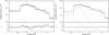 |
Fig. 1 Fitted combined/total Chandra ACIS-S3 spectrum of T Pyx. Left panel: fit with the tbabs×CEVMKL model; right panel: fitted tbabs×(MEKAL+MEKAL) model. The crosses are the data with errors, solid lines are the fitted model, and dotted lines show the contribution of the models. Lower panels: residuals in standard deviations (in sigma). |
Spectral parameters of the total (combined) spectrum of T Pyx (0.2−9.0 keV).
The X-ray spectra of nonmagnetic CVs is found to show a temperature distribution of hot optically thin plasma emission as the accreting gas settles on the WD through the boundary layer revealing several emission lines detected ranging from H- and He-like elements to Fe L-shell lines (Mukai et al. 2003; Baskill et al. 2005; Pandel et al. 2005; Guver et al. 2006; Okada et al. 2008; Balman et al. 2011; Balman 2014). These spectra are well modeled with an isobaric cooling flow that is a multitemperature distribution of plasma with differential emission measure assuming power-law distribution of temperatures (dEM = (T/Tmax)α − 1dT/Tmax; e.g., MKCFLOW or CEVMKL within XSPEC software).
The combined spectrum of T Pyx cannot be fitted with a single-temperature component plasma emission model in collisional equilibrium or a blackbody model, with  values much larger than 2. Figure 1 shows the total spectrum of the source which portrays a smooth continuum-like characteristic. This is due to the low count rate of the source which yields only about 510 net source counts in the total ~100 ks Chandra observation. For any given plasma model with near-solar composition and moderate emissivity from lines convolved with moderate spectral resolution of the ACIS-S detector (with no gratings in use), these features may be smeared out and superimposed over the continuum. Therefore, nondetection of particular emission lines are expected.
A (cooling flow-type) multitemperature distribution plasma model, (with a power-law distribution of temperatures) CEVMKL in XSPEC, was used to model the spectrum of T Pyx in accordance with the general concensus of the X-ray spectra of nonmagnetic CVs as mentioned in the previous paragraphs. The fit result yield 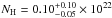 cm-2,
cm-2,  keV,
keV,  (power law index of the temperature distribution) and the normalization is 4.4
 × 10-5 (see Table 1 and Fig. 1a). The unabsorbed X-ray flux is (5.0 − 8.0) × 10-14 erg s-1 cm-2 in the 0.2−9.0 keV range which translates to a luminosity of (0.8−1.2) × 1032 erg s-1 (at 3.5 kpc source distance). The flux and luminosity are (0.9−1.5) × 10-13 erg s-1 cm-2 and (1.2 − 2.2) × 1032 erg s-1 in a wider energy band of 0.1−50.0 keV. The maximum X-ray temperature has a very high unconstrained best-fit value of kTmax> 47 keV with a 2σ lower limit of 37 keV. The power law index α of the X-ray temperatures diverges somewhat from 1.0 (an index α of 1.0 is expected from an isobaric cooling flow-type plasma). The NH value derived from the fit is consistent (at 95% confidence level) with the interstellar value derived for T Pyx using nhtot, 0.28 × 1022 cm-2 from the database of Willingale et al. (2013)1 who use the atomic hydrogen column density, N(HI), and the dust extinction, E(B − V), describing the variation of the molecular hydrogen column density, N(H2), of our Galaxy, over the sky using 21 cm radio emission maps and the Swift GRB data. The measured value of E(B − V) = 0.5 − 0.25 (higher limit from Shore et al. 2011: during outburst, lower limit from Schafer et al. 2013: during quiescence) yields a range of NH = (1.5 − 3) × 1021 cm-2 consistent with the nhtot result and the derived spectral parameter NH in Table 1.
The normalization of the CEVMKL model is similar to MEKAL assuming an average emission measure (EM; see also Table 1). Taking a distance of 3.5 kpc and that ⟨ EM ⟩ = ⟨ ne ⟩ 2V (V = emitting volume), an electron density can be approximated. For an emitting volume of (3 × 109 cm)3 for simplicity, the best-fit value of the normalization gives an average electron density of 1013 cm-3. This density yields equipartition of temperature between electrons and ions (CIE) in about 10 s assuming 37 keV temperature, and if the temperature is lower the equipartition is faster (equipartition timescale from Fransson et al. 1996). During the fitting process a solar plasma composition was assumed. When the abundances are set free in the CEVMKL fits, some overabundances in the elements are seen but not detected with any significance and the of the fit is not altered. I have also checked the general metal abundances using the CEMEKL model (CEVMKL without individual abundances). Such a fit yields almost the same spectral parameters as in the CEVMKL model fit with the additional parameter range of metal abundance of 0.4−2.3 (90% confidence level) for the quiescent spectrum of T Pyx. In general, I note that the X-ray temperature is very high and the power law index of the temperature distribution slightly diverges from an isobaric cooling flow for an optically thin hard X-ray emitting boundary layer. At the accretion rates of T Pyx Ṁ> 10-8M⊙ yr-1, the boundary layer is expected to be in the optically thick regime (see Popham & Narayan 1995; Popham 1999).
A double plasma emission model can be fitted with around 1.0 yielding spectral parameters; an NH of 0.3 cm-2, a kT1 of 0.25
 , a normalization 4.0
 , and a kT2 of 79.0
 keV with a normalization of 3.7
 (errors are given at 90% confidence level). The integrated unabsorbed X-ray flux is (5.0 − 9.0) × 10-14 erg s-1 cm-2 in the 0.2−9.0 keV range which translates to a luminosity of (0.8 − 1.4) × 1032 erg s-1 (at 3.5 kpc source distance). This fit is shown in Fig. 1b. The flux and luminosity are (0.8 − 2.3) × 10-13 erg s-1 cm-2 and (1.1 − 3.4) × 1032 erg s-1 in a wider energy band of 0.1−50.0 keV. These values are similar to the ones derived in Balman (2010) from the XMM-Newton data except that there is no need for two different NH to fit the total Chandra spectrum. The NH value derived from the fit is consistent with the interstellar values as in the previous fit. The physical interpretation of the two thermal plasma component fit may be an indication of the multitemperature nature of the plasma in the boundary layer or that there are two different contributing X-ray emission regions. This will be discussed later.
The combined total spectrum of T Pyx can not be satisfactorily interpreted in the context of a standard nonmagnetic CV. For a nonmagnetic CV, the virial temperature in the inner parts of the accretion disk (kTvirial = μmpGMWD/ 3RWD) is kTvirial = 20 − 29 keV for a 0.7−1.0 M⊙ WD (WD mass is from Uthas et al. 2010; and Toffelmeier et al. 2013). The X-ray temperatures in Table 1 show that the flow is already virialized. A cooling flow-type plasma releases an energy of (5/2)kTmax per particle including kinetic and compressional components. The total thermal/kinetic energy at the inner edge of the disk per particle is (3/2)kTvirial. Thus, the plasma maximum temperatures in the cooling flow are limited with (Tmax/Tvirial< 3/5) yielding a Tmax of about 12−18 keV. The X-ray temperature values (obtained from the total spectrum) of T Pyx are higher than this limit. Therefore, the Chandra observations of T Pyx are not satisfactorily explained in the context of optically thin boundary layers in quiescent dwarf novae or in the context of theoretical expectations from optically thick boundary layers. This will be elaborated in Sect. 4.
It has been suggested that the source in T Pyx is nonthermal (Scheafer et al. 2013). I have also fitted a power-law model to the total spectrum to confirm such an expectation. The spectral parameters of the fit are an NH fixed at the interstellar value 2.0 − 3.0 × 1021 cm-2, a photon index of 1.6 and a normalization of 7.6
 ( = 1.71 (d.o.f.17)). The of the fit is worse than the fits with the thermal plasma models at 98.5% confidence level (almost at 3σ) and can be excluded. I note that the NH is fixed during the fitting process because it can not be constrained yielding values that are too low. This may be a result of the unresolved contribution of line emission superimposed over the continuum. In such a case the continuum level is elevated and a simple continuum model such as power law will still fit the spectrum, but at a higher normalization, which will have the effect of lowering the NH parameter in the presence of constant interstellar NH absorption.
Spectral parameters of the extended nebular spectrum of T Pyx (0.2–9.0 keV).
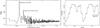 |
Fig. 2 Left panel: PSD obtained from averaged power spectra of the three observations. Right panel: folded average X-ray light curve of T Pyx using the detected binary period. |
The smooth featureless Chandra spectrum of T Pyx suggests plausible non-equilibrium ionization (NEI) plasma effects. A simple model of VNEI in XSPEC can be used to check this further. The model gives acceptable fits with the data only if NH is set free and yielding an ionization parameter  cm-3 s (τ = nt, n is electron density in this case). Using the normalization of the fit which is the same as the CEVMKL model, a similar electron density ~1013 cm-3 can be calculated. A double check of these model parameters yields an ionization timescale on the order of milliseconds and thus a VNEI model is not physical for this data. Non-equilibrium ionization models like Comptonized plasma models (e.g., CompTT, NthComp in XSPEC) give consistent fits with the spectrum of T Pyx only if NH is set free yielding much lower values than the interstellar NH. This problem is removed (fit improved at 3σ, CompTT is used) if NH is fixed at the interstellar value and a second thermal MEKAL model is added to the fit (a blackbody model is inconsistent) giving a fitted temperature of 0.2−0.55 keV for the MEKAL model with Comptonized plasma temperatures 3.0−27.0 keV and electron scattering optical depth 2.0−8.0 (errors are at 90% confidence level). The temperature of the MEKAL model is very similar to the first plasma temperature of the double MEKAL model fit in Table 1 (see also Table 2). In this case (inclusion of a MEKAL component), a power-law model may also yield acceptable fits. Since there are no current models that describe Comptonized plasmas for nonmagnetic CVs (and WDs), no further elaboration will be included, but there is consistency with the existing Comptonized plasma emission models.
Selvelli et al. (2008) and Balman (2010) discuss how the blackbody model of emission is inconsistent with the data. A 2σ upper limit on the soft X-ray emission from T Pyx calculated from the spectral fits to the Chandra data using the blackbody model is a of kTBB< 25 eV and fBB< 1.5 × 10⁻¹² erg s-1 cm-2 in the 0.1−10.0 keV range. The upper limit on the flux yields a 2σ upper limit on the soft X-ray luminosity of Lx< 2.0 × 1033 erg s-1 (using 3.5 kpc distance and 0.1−10.0 keV range).
3.2. Temporal variations of the central source
I created background-subtracted light curves with the aid of the CIAO task dmextract to search for any time variability. The three light curves were used to generate averaged power spectra (PDS). I find significant modulation at the binary period of the system (and its second harmonic) above 99.9% confidence level where 3σ power threshold is >77 taking into account the red noise in the PDS around the binary period and its harmonic. The binary period is 1.8295(3) h; 0.152 mHz (Uthas et al. 2010). I do not detect any other periodicity. The PDS with the detected period of 0.155±0.005 mHz is shown in Fig. 2, and the folded average light curve is given in the right panel of the same figure. There is a constant level of emission in the folded light curve at about ~0.003 c s-1. Superimposed on this constant level, there is variation between 0.003 c s-1 and 0.008 c s-1 with a mean, net, count rate ~0.0025 c s-1 yielding a percent modulation in semi-amplitude of about 45% ([max-min/max+min]×100).
Energy dependence of these orbital modulations are studied using light curves in the 0.2−1.0, 1.0−2.0, and 2.0−7.0 keV energy bands. Aside from the changing average count rates in the energy ranges, the modulations and the shape of the average light curve are unaltered. There is no energy dependence in the orbital modulations in the Chandra energy band. T Pyx shows orbital modulations in the X-rays during the outburst stage with a slightly different shape of the (folded) mean light curve (Tofflemire et al. 2013).
 |
Fig. 3 X-ray images of T Pyx Nebula in the 0.2 to 7.0 keV range. North is up and west is to the right. Left panel: vicinity of the source within 15 arcsec radius and the photon extraction radii for the source and background are overlaid for 5 and 2.5 arcsec. Middle panel: image without the subtraction of the central source PSF. Right panel: PSF-subtracted image. The resolution is 0.̋25 per pixel in the right panel. The axes on the figures show RA (x-axis) and Dec (y-axis). The images utilize different brightness levels using the square root scaling. |
3.3. On the extended emission around T Pyx
A low signal-to-noise ratio (S/N ~ 4−5σ) extended excess emission was recovered in the XMM-Newton data of T Pyx (Balman 2010). In order to assess this better, a long observation of T Pyx was obtained in quiescence with a much better spatial resolution capability. To improve the spectral statistical quality and effectively recover the extended emission using deeper imaging, the three Chandra observations of T Pyx (see Sect. 2) were merged with the standard procedures2. A specific new tangent point (RA-Dec: 09 04 41.49, −32 22 47.65) is used to match the three OBSIDs which projects the events to the nominal point of ACIS-S (x = 4096.5, y = 4096.5 in WCS–World Coordinate System) for all three observations in the process of the analysis. Thus, the events in the three observations have been reprojected to this new tangent point and the analysis is performed at/around the nominal point of ACIS-S. During all of the re-projection processes in my analysis pixel randomization was turned off. In addition, all events files have been re-processed (using acis-process-events) without randomization of any kind (pix-adj=NONE, yielding original position of detected photons). In general, I have analyzed the T Pyx data originally generated in 2011 (processed with pixel adjustment set to randomize using 0.5 pix) and archived in 2012 (processed with pixel adjustment set to EDSER, a new event repositioning algorithm to improve pixel resolution) and found similar results (using pix-adj=NONE). In merging events, there are two important factors, one is the fine astrometric shifts that are necessary to match sources, the second is the choice of a common tangent plane as used in this analysis with the assumed new RA-Dec position to project all the events files. To improve on any systematic shift in the coordinate systems between observations and enable usage for high-resolution imaging at the subpixel level of the combined data sets, the aspect solutions of the observations have to be corrected to make them consistent with each other. Certain astrometric shifts were determined for the correction of the aspect solutions and applied as described in the analysis threads, updating WCS and re-projecting the events matching them to the second observation of T Pyx. In this analysis, shifts were calculated using the projected events files to the nominal point of ACIS-S and also checked with the shifts obtained from the original individul data sets. The results show that the shifts in the x- and y-axis for the first and the third observations are in a range ≤±0.5 pixels including errors. The range is a result of different radii chosen for dmstat to calculate centroids for the source yielding slightly different shifts for different radii from a given observation. The shifts used in this study are x = 0.5 pix, y = −0.07 pix for the first observation (ID 12399) and x = 0.04 pix, y = 0.03 pix for the third observation (ID 13224). The shift variations may be due to the imperfect source profile caused by the superimposed extended emission with a different symmetry (see discussions in the following paragraphs). Using these astrometric shifts obtained from a given source radii (5−7 pix) yields similar structure at around the nominal point, however slightly defocused (slightly unmatched). I have tested the data for several sets of shifts and using small extra systematic shifts in the given range of shifts in pixels keeping track of bright parts and the elongation towards south in the individual images to match them in the final merged image. The shifts given above for this study are final shifts used in the analysis. Mainly, one needs to do only one re-projection of the individual events files to the nominal point using a new tangent point (RA-Dec) as one starts the analysis with and next apply astrometric shifts to match these events files. In general, all throughout the analysis the location of the nominal point and the chosen RA-Dec position should remain intact. If any slight miss-match occurs, in this case a second re-projection of the shifted events should be done using the event file of the observation chosen as reference for the other two observations (second observation in my case). This process corrects the match between sky coordinates and WCS and thus, the location of the nominal point (and puts the data on common tangent planes). However, it leaves the profile of the source unaltered from the profile with the inadequate shifts and the incorrect aspect solution calculated with these inadequate shifts. Therefore, care must be taken to check allignment at every step of the analysis.
To create the PSF, the CHART ray tracer was utilized using the necessary off-axis angles (taken from the merged event file), the combined source spectrum (see Sect. 3.2) and the entire exposure time (98.8 ks). Next, MARX version 4.5.0 was used to project the PSF rays onto the detector plane and finally an events file was generated for the source PSF. A single PSF was generated for the analysis to ensure no centroiding/allignment problems for the PSF. The three observations were obtained within one week’s time and a single PSF, thus is suitable. In addition, all three observations are pointed near by and have no off-axis angles larger than 20 arcsec where the standard PSF is mostly unaltered. Since the combined source spectrum, thus source flux is directly used with the exposure time, the created PSF is expected to be very similar to the combined/merged Chandra observation of the source. For the analysis several PSFs were generated and inspected. It has been calculated and checked that in the same size region at round the PSF kernel size both the simulated PSF data and the source data images yield very similar photon counts around 510 ± 15. This means that no further secondary normalization can be made on the PSF without changing the constant source flux that is in the data and the simulated data (PSF). If there is a necessity, a new PSF should be recalculated instead of a secondary normalization for simulated PSF and source data correspondence. Moreover, images derived from these two event files (source data and simulated PSF data) have to be treated exactly the same way in any analysis so that this correspondence of flux/counts remain the same. In addition, I stress that PSF events files have no aspect solutions that can be properly used for astrometric corrections to match and use particularly with high-resolution imaging analysis at the subpixel level, as in the standard events files. Therefore, merging PSFs needs to be cautioned for subpixel imaging analysis. I also note that in this analysis the individual PSF events files have to be projected to the nominal point for any subtraction process where aspect solution files will be necessary.
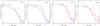 |
Fig. 4 Surface-brightness radial profiles of the source T Pyx extracted from a sector-area of opening angle 30 degrees. From left to right: profiles are in the eastern, western, northern, and southern directions. In all panels, an equivalent Chandra ACIS-S3 PSF radial profile of about 500 photons calculated from the same sector is overplotted. Gaussian errors are assumed. |
Since the standard Chandra pixel resolution did not properly resolve the structure of the extended emission (see the discussion of the 1D radial profiles later in this section), a 0.1 pixel scale (corresponding to a 0.̋05 angular size) was used to push the spatial resolution of the data close to the instrumental limit for a detailed imaging analysis. I note here that the photon positioning capability of Chandra is good, but the caveats due to the detector, HRMA and aspect errors results in a substructural resolution of Chandra ACIS-S no better than 0.̋2−0.̋3. Therefore, structure sizes smaller than this can not be resolved. Moreover, I stress that there is no study or known calibration work done to test the subpixel response of the PSF at off-axis angles (private communication with the Chandra Calibration team through HelpDesk). Therefore, it is most suitable to do the analysis at around the nominal point of ACIS-S where resolution is best, well known, and well calibrated. Then, the choice of merging the three events files of T Pyx via a new tangent point RA-Dec that projects the events to the nominal point is the correct choice.
During the high-resolution imaging analysis of T Pyx at the subpixel level, a slow PSF subtraction methodology is used. The data image and the PSF image created with the same 0.1 ACIS pixel scale in the 0.2−7.0 keV band with matching coordinates were subtracted in iterative steps. First, with no smoothing applied before subtraction, then with 1 × 1 pixel smoothing applied before subtraction, finally 2 × 2 pixel smoothing applied before subtraction while a persistent structure remaining in the PSF-subtracted data images is explored. A Gaussian smoothing is used with the task csmooth. The task csmooth (an adaptive smoothing technique) is run with constant/same minimum and maximum smoothing pixels. Non-integer values of pixel smoothing were used to check how well the iterative process works.
The resulting image after PSF-subtraction (using the 1×1 pixel smoothing) was further smoothed by 2×2 pixels yielding a spatial resolution of 0.̋25 and shown in Fig. 3 (right hand panel). The left panel of Fig. 3 shows the 15 arscec vicinity of T Pyx, and the middle panel shows the unsubtracted subimage derived from the merged events file. Note here that, smoothing decreases spatial resolution since it re-evaluates the data values in the images at given subpixel positions and increasing smoothing makes the resolution closer to the standard pixel images of Chandra ACIS-S.
The PSF-subtracted final image indicates some extended emission with an elliptical shape. The outer semi-major axis is ~1.̋0 and the outer semi-minor axis is ~0.̋5. I emphasize that the subtraction process also yields a depression of counts at the center, which is expected if the PSF and the data image is correctly normalized; size of this depression in counts is about 0.̋2−0.̋4 at the substructural resolution limit. This possibly indicates a torus-like or ring-like structure around the nova. In addition, there seems to be an elongation towards the south to about 1.̋85 from the point source. The southern region of extension comprises about 13% of the extracted X-ray nebulosity. I checked the consistency of the X-ray nebula by analyzing the three datasets of T Pyx and subtracting an appropriate PSF from each individual image. Though the S/N is low, structures resembling Fig. 3 were seen. In addition, I checked the given PSF subtraction procedure with some weak sources that show no pile-up and found no excess structure as in T Pyx. My experience in these trials has been that the PSF image clears the source data image more or less using 1×1 pixel smoothing before subtraction (at 0.1 ACIS pixel scale) leaving behind no definite structure but some scattered spots.
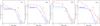 |
Fig. 5 Surface-brightness radial profiles of the source T Pyx extracted from a sector-area of opening angle 30 degrees. From left to right: radial profiles are in the eastern, western, northern, and southern directions. A Chandra ACIS-S3 PSF radial profile of about 250−300 photons calculated from the same sector is overplotted for comparison with Fig. 4. Gaussian errors are assumed. |
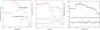 |
Fig. 6 Left panel: combined/total spectrum of the source plus the nebular emission in the X-rays (in red) and the nebular X-ray spectrum of T Pyx (in black). Middle panel: fit of a single componant plasma model to the X-ray nebular spectrum and the residuals in sigmas. Black denotes the spectrum derived from the 2×2 pixel smoothed images (also on the left) and the red spectrum is the one derived from the 3×3 pixel smoothed images. Right panel: Chandra ACIS-S3 combined spectrum fitted with (tbabs*(MEKAL+CEVMKL)+tbabs*MEKAL) model of emission. The dotted lines show the contribution of the three fitted models, two of which fit the X-ray nebular spectrum and the third fits the central source spectrum. The lower panel shows the residuals in standard deviations (in sigma). |
I determined an approximate nebular and point source count rate by using the PSF-subtracted total image (merged) of the nebula within about a radius of 5′′ (the circular extraction area is shown in Fig. 3a; the large circle), since it is about the size of the optical remnant (see Schaefer et al. 2010) and the Chandra nebulosity is within 2′′ of the point source. As in the imaging analysis discussed/outlined above, I used either no smoothing or 1×1 pixel and 2×2 pixel smoothing for both the PSF and the merged source image with the 0.1 ACIS pixel scale to obtain an approximate nebular count rate. I used a similar size photon extraction region obtained elsewhere in the image to account for the number of background photons (the extraction area is shown in Fig. 3a; the large circle on the right). This analysis yielded an approximate count rate of (0.0023±0.0010) c s-1 (about 40% error) for the extended emission and ~0.003 c s-1 for the central source over the 0.2−7.0 keV energy range (the rates indicate no concerns for pile-up). Because of the caveats of the high-resolution imaging analysis at the subpixel level, it is very likely that the lower half of the count rate range, ~(0.0013−0.0025) c s-1, is plausibly more representative of the X-ray nebular emission. The S/N of the extracted nebulosity is between 6−15 using the entire range of the X-ray nebular count rate (~6−10 for the lower half of the count rate that is a better estimate of the S/N) (S/ ; E is the net nebular counts, B is the background counts, and P is the counts in the PSF).
In order to inspect the morphology of this nebulosity, radial profiles of T Pyx are calculated in different directions and are shown together with the radial profile of the simulated PSF used for the analysis in Fig. 4. For the analysis, the task dmextract is used along with the circular annuli within a region of about 3′′ radius to indicate the background (Gaussian errors are assumed in the calculations). The total number of photons are about the same in the source and PSF profiles. The T Pyx radial profiles are created from a sector with a narrow opening angle of 30 degrees centered on the east, west, south, and north. A radial profile of the ACIS-S3 PSF with about the same number of photons as in the source radial profile calculated from the same sector with the given directions is included in all the figures. Gaussian errors are assumed. The extended nebulosity in the western part is evident. Moreover, the northern profile is narrower than the PSF indicating that the underlying central point source has less emission and thus consistent with a smaller PSF. The southern profile is larger in extend than the PSF indicating the existence of some southern elongation as shown in Fig. 3. The excess in the central part of the southern radial profile is consistent with the excess in the northern sector and is originating from the superimposed elliptical nebulosity as projected mainly on the minor axis. Therefore, one needs to be very careful in interpreting circularly symmetric radial profiles where superimposed noncircular and/or local geometries may not show explicitly in a total 1D circular radial profile. In order to show the compliance of the T Pyx radial profiles with point source PSF with less counts than the total counts detected from T Pyx, I prepared similar figures using the same source radial profiles from a sector of 30 degrees, but this time overlayed point source PSF with counts in the range of 250−300. Figure 5 shows the correspondence with total counts from a smaller point source. Particularly, the eastern and northern radial profiles yield consistent results with a smaller point source size. There is an excess superimposed on the central regions in all the figures in Fig. 5 (and Fig. 4). I suggest that this may result from an elliptical nebulosity superimposed on the semi-minor axis (~0.̋5).
An Astronomer’s Telegram3 (ATEL) on this Chandra data claims that the extended emission is due to an HRMA artifact (Montez et al. 2012). The HRMA artifacts for weak sources like T Pyx are less than 5% of the total emission (private communication with the CXC calibration team through the HelpDesk) and are from a very localized region of 0.̋6 by 0.̋44. The entire size of the X-ray nebula, as I have derived, is much larger than an artifact zone and the nebular emission is about or more than 30% of the total emission from the source showing that it is not an HRMA artifact. Moreover, the extension towards the south is also about 13% of the total source emission. The artifacts should be looked for in the original data and images and not in the images from reprojected and merged events files as in Montez et al. (2012) since WCS is also updated during the projection process. Reprojection and merging of events do not create HRMA artifacts. Analyses of the original data sets (using CIAO task make-psf-asymmetry-region) yield zero photons in the first data set, six photons in the second dataset and seven photons in the third data set of T Pyx, that operlap with the HRMA artifact regions which totals to 16 photons that may be associated with an artifact. Thus, there are no concerns from significant contribution of HRMA artifacts into the nebulosity. Moreover, the radial profile presented in this ATEL is in “counts” and shows definite misallignment. The unit “counts” is not surface brightness in “counts/pixel2” and the extraction area increases as you go from the center of the PSF/source to the wings of the profiles. Therefore, there is a normalization problem and a definite 0.3−0.4 arcsec positional centroid mismatch between the merged PSF and the merged T Pyx profile in Montez et al. (2012) which does not exist in Figs. 4 and 5 in this paper.
3.4. Deconvolution of the Chandra spectrum of the X-ray nebula and the central source
The excess nebulosity around T Pyx and the inadequate results from the analysis of the total/combined spectrum possibly support the existence of two different origins of emission within the total spectrum; one being the CV which is the point source and the other the X-ray nebula. The nebular emission is within 2.̋5 of the point source (about 1′′ radius) and it is weak compared to the point source. As a result of the difficulty of extracting photons from separate regions to collect nebular photons and source photons at around the subpixel level, I used the technique described below to deconvolve the two spectra: I have assumed 16 equal energy channels between 1−1024 channels of the Chandra ACIS-S (e.g., 1−63, 64−127, 128−191... 512−575). For each of the given 16 energy channel ranges, subimages were created using the merged events file and the PSF events file as used in the imaging analysis of the previous section. The PSF and the source images created at the given energy channel ranges were smoothed by 2×2, or 3×3 pixels, where each pixel was at 0.1 ACIS pixel scale (using a Gaussian kernel). Next, PSF images were subtracted from the source images using the same ACIS pixel scale, smoothing, and matching coordinates. The resulting PSF-subtracted images were thresholded to have zero counts for the negative pixel values. Using these subtracted images, the number of counts in each channel range (representing the excess nebular counts) were calculated utilizing the same photon extraction radius as the combined source spectrum (either 5′′ radius with the 2×2 pixel smoothed images or 2.̋5 radius with 3×3 pixel smoothed images have been used). The 5′′and the 2.̋5 photon extraction radii for the source and background are shown in Fig. 3a. The nebular spectrum was created by replacing the counts in the re-binned combined spectrum (re-binned to have 16 channels) created using 5′′ or 2.̋5 photon extraction radius. The same background spectrum is used for the nebular spectrum as derived for the combined total spectrum assuming the corresponding photon extraction radius. Figure 6, left panel, shows the nebular spectrum with the 2×2 pixel smoothed image subtraction in comparison with the total combined spectrum. The middle panel shows both of the nebular spectra that use the 2×2 pixel smoothed image subtraction (in black) and 3×3 pixel smoothed image subtraction (in red).
The deconvolution method used here has some caveats. The first one being the low counts in the selected energy channels which may result in an appreciable mismatch between PSF and source photon positions within the PSF kernel. The choice of background and extraction radius may also yield slight variations of the calculated nebular spectrum. As described above, to mitigate this, 2×2 pixel (0.̋25 resolution), or 3×3 pixel (0.̋35 resolution-larger than half the standard Chandra pixel) Gaussian smoothing was used for the imaging analysis. It is evident that similar spectra were derived, but, I emphasize that as the counts get lower in the harder energy channel ranges, the image subtraction is relatively less reliable. On the other hand, I stress that completely smoothed out images were subtracted in all the energy channel ranges.
The deconvolved approximate nebular X-ray spectrum was modeled using a two-component plasma emission model (in thermal equilibrium) with two different hydrogen column densities since a single plasma model or a single absorption component yielded larger than 2 (see Fig. 6 middle panel). However, the second thermal component and thus, the high absorption between two components are found from a self-consistent analysis across all selected energy channels, but need to be taken with caution as a result of the described caveats in the previous paragraph. Table 2 shows the spectral parameters for two-component plasma model fits with a MEKAL model (assuming collisional equilibrium) and a PSHOCK model (assuming NEI). The fits yield similar parameters. The ionization timescales derived from the PSHOCK model indicate existence of NEI plasma, but the parameter can not be constrained allowing for ionization equilibrium. The spectral results (e.g., double MEKAL) indicate an absorbed X-ray flux of (0.3−10.0) × 10-14 erg s-1 cm-2 which translates to an X-ray luminosity of (0.6 − 30.0) × 1031 erg s-1 at the source distance of 3.5 kpc. The count rate error of 40% in the subtraction of the nebular component is quadratically added to the normalization, flux and luminosity.
To determine the approximate central source spectrum (the binary), I fitted the combined spectrum with a composite model (tbabs*(MEKAL+CEVMKL)+tbabs*MEKAL). The two MEKAL models (with the two different absorption models) represent the nebular spectrum and the CEVMKL is used to model the central binary spectrum typical of accreeting nonmagnetic CVs. The nebular spectrum parameters are slightly varied around their best-fit values (the lower plasma temperature of the nebula and the NH2 is slightly varied) during the fitting procedure. The fitted combined spectrum is shown in the right panel of Fig. 6. Using the CEVMKL model, the spectral parameters of the central source are a kTmax> 14.0 keV, and a normalization of 5.1 for the spectrum of the central source emission (the power law index of α for the temperature distribution was fixed to 1.0). This yields an unabsorbed X-ray flux of (2.0−7.0) × 10-14 erg s-1 cm-2 with a luminosity of (2.9−10.3) × 1031 erg s-1 (0.2−9.0 keV) (40% error in the subtraction of the nebula is quadratically added to the normalization, flux and luminosity). The NH parameter is the same as in Table 1. The of the fit with the CEVMKL model for the central source spectrum is 0.6. For the sake of the caveats mentioned on the second component of the nebular emission, I have assumed only the first low temperature component of the nebular spectrum omitting the second component and fitted the combined spectrum to check the central source spectral parameters. The CEVMKL fit yields kTmax> 39 keV (α fixed at 1.0) with a similar range of interstellar NH together with flux and luminosity in a similar range to the analysis in Sect. 3.1 (given inclusion of the 40% error in the subtraction of the nebula).
4. Discussion
4.1. Central source/binary
I have presented the pre-outburst spectral and temporal analysis of T Pyx in quiescence obtained around Feb. 2011 in three 30 ks observations within about a week of each other. The total spectrum of the combined three datasets yields hard X-ray plasma emission from the source with an X-ray temperature of kTmax> 47.0 keV (a 2σ lower limit from the CEVMKL fit is 37 keV), an NH of 0.1 cm-2 and an unabsorbed X-ray flux of (5.0 − 9.0) × 10-14 erg s-1 cm-2 with a range of X-ray luminosity (0.8 − 1.4) × 1032 erg s-1 in 0.2−9.0 keV band. In a wider range of 0.1−50 keV the integrated flux and luminosity are (0.9 − 1.5) × 10-13 erg s-1 cm-2 and (1.3 − 2.2) × 1032 erg s-1, respectively. A multitemperature plasma emission model, CEVMKL, is assumed for the fit in accordance with modeling of the nonmagnetic CVs in quiescence. A double MEKAL model is also consistent with the total X-ray spectrum, reflecting that the plasma temperature is already a multitemperature distribution. On the other hand, the lower plasma temperature resembles the temperature of the extended nebulosity recovered from the source in this work and also using XMM-Newton which may belong to a different origin. I note that the combined spectrum show consistency with Comptonized plasma emission models, and they reveal a second thermal plasma component with a temperature in accordance with the low temperature of the extended nebulosity.
The optical V band magnitude of T Pyx was in a range 15.4−15.6 in 2006 during the XMM-Newton and in 2011 during the Chandra observations (using available AAVSO data). Thus, the system brightness has not changed much in the optical band, which otherwise might have signaled a noticeable change in the accretion state. The comparison of the total X-ray flux (unabsorbed) and the X-ray luminosity of the central source in T Pyx (in the 0.2-10.0 keV range) indicates that there is a definite overlap of the flux ranges calculated for the source in 2006 (XMM-Newton) and 2011 (Chandra) observations since the error on the unabsorbed flux in XMM-Newton data is large and between (3.0−80.0) × 10-14 erg s-1 cm-2.
A complicated deconvolution of the central source spectrum (see Sects. 3.3 and 3.4) was applied to the data to extract any extended X-ray nebulosity from the central source emission; the results indicate that the X-ray temperature of the central source is still hot with kTmax> 14 keV (best fit results using a CEVMKL model). The maximum temperature of the plasma temperature distribution is unconstrained. The corrected unabsorbed flux and luminosity are (0.7−7.0) × 10-14 erg s-1 cm-2 and (1.1−10.0)×1031 erg s-1, respectively. This luminosity and flux are (3.0−12.0) × 10-14 erg s-1 cm-2 and (4.4 − 18.0) × 1031 erg s-1 in the 0.1−50 keV energy range.
I do not find a blackbody emission component consistent with (satisfactorily fitting with significance) the Chandra pre-outburst spectra as was detected with XMM-Newton (Selvelli et al. 2008; Balman 2010) and ROSAT (RASS data; Greiner & Di Stefano 2002) in the earlier studies over the years (there is no super soft X-ray source (SSS) associated with T Pyx in quiescence). As mentioned in Sect. 3.1, there is no intrinsic absorption in the system, but absorption only at the interstellar value. I exploit the data to calculate a 2σ upper limit to temperature and flux for the blackbody emission from T Pyx as kTBB< 25 eV, fBB< 1.5 × 10⁻¹² erg s-1 cm-2 and LBB< 2.0 × 1033 erg s-1 in the 0.1−10.0 keV band.
Gilmozzi & Selvelli (2007) have studied the UV spectrum of T Pyx in detail and found that the SED is dominated by an accretion disk in the UV+opt+IR ranges, with a distribution, described by a power law Fλ = 4.28 × 10⁻⁶λ-2.33 erg s-1 cm-2 Å-2, while the continuum in the UV range, alone, can also be represented by a single blackbody of T ~ 34 000 K. The observed UV continuum distribution of T Pyx has remained constant in both slope and intensity during 16 years of IUE observations. Selvelli et al. (2008) predict a disk luminosity of about 3×1035 erg s-1 (from UV and optical bands) for T Pyx consistent with the accretion rate they calculate in the optical and UV regimes (1−4)×10-8M⊙ yr-1 for a WD mass of (0.7−1.4) M⊙. I note that larger accretion rates of (1 − 10) × 10-7M⊙ yr-1 have been suggested for T Pyx as well (Schaefer et al. 2013; Godon et al. 2014). In this accretion rate range, the nature of the boundary layer should be discussed in the framework of the calculations of the standard steady-state disk models expected for CVs (e.g., of Narayan & Popham 1993; Popham & Narayan 1995; Popham 1999). These models predict optically thick BLs with blackbody temperatures of 13−33 eV and Lsoft ≥ 1 × 1034 for 0.8−1.0 M⊙ WD (a rotation as high as Ω∗ = 0.5ΩK(R∗) is already assumed in luminosity/temperature limits) which I did not recover using the Chandra data. I emphasize here that the standard nova theory predicts near-Chandrasekhar masses for the WDs in RNe and this predicted mass value implies much hotter and X-ray luminous optically thick boundary layer for T Pyx than these given range limits.
Detailed calculations by Narayan & Popham (1993) show that the optically thin BLs of accreting WDs in CVs can be radially extended and that they advect part of the internally dissipated energy as a consequence of their inability to cool, therefore indicating that optically thin BLs act like advective hot accretion flows (i.e., ADAF-like: advection-dominated accretion flow). In addition, Popham & Narayan (1995) illustrates that the BL can stay optically thin even at high accretion rates (as for T Pyx) for optical depth τ< 1 together with α ≥ 0.1. However, nature of such models have not been well investigated. An ADAF around a WD can be described by truncating the ADAF solutions at the WD surface as opposed to BHs and the accretion energy is advected onto the WD heating it up. Medvedev & Menou (2002) and Menou (2000) include some preliminary work regarding ADAF-like flows and hot settling flows in CVs (dwarf novae) where Menou (2000) suggests that ADAF-like gas flows in the BLs of CVs are expected to be one-temperature in CIE since Coulomb interactions at low temperatures compared with BH binaries are efficient and advection does not depend on preferential heating of the ions by viscous dissipation and lack of energy exchange between electrons and ions necessary for two-temperature flows as in BHs (NEI). However, since there are no detailed calculation of ADAF-like flows for CVs in general the two-temperature flows can not be completely ruled out. Recently, Balman et al. (2014) have shown that some Nova-like CVs have BLs that can be characterized with ADAF-like flows merged with optically thin BLs in high state CVs. These objects have accretion rates similar to or somewhat less than T Pyx. The X-rays have optically thin multiple-temperature cooling flow type emission spectra with temperatures kTmax in a range 21−50 keV. These BL regions are also found to be divergent from the isobaric cooling flow models and the temperatures are at/around virial values with similar characteristics to quiescent X-ray emission of T Pyx.
Given the disk luminosity mentioned previously for T Pyx and the X-ray luminosity in the 0.1−50 keV range the ratio (Lx/Ldisk) ≃ (2 − 7) × 10-4. The nature of the boundary layer in the central source in T Pyx is not consistent with the predictions from the calculations of the standard steady-state disk models (Lx ~ Ldisk) (e.g., Narayan & Popham 1993; Popham & Narayan 1995). I note that discrepancy between Lx and Ldisk is common for nonmagnetic CVs and this ratio has been found to be around 0.1 for SU UMa-type dwarf novae and about 0.01 for the U Gem subtype together with the nova-likes at high states having a ratio of around 0.001 (see Kuulkers et al. 2006 for a review). The expected soft X-ray/EUV emission is not detected from the BL region and the accretion flow is most likely virialized and very hot and optically thin as discussed in Sect. 3.1. I suggest that the X-rays from the point source originate in an optically thin boundary layer that is merged with an ADAF-like flow and/or in an accretion disk coronal region where accretion occurs through hot coronal flows onto the WD. Such a quasi-spherical/torus-like hot accretion flow in the BL zone may also obscure the WD even at low inclination angles.
In X-ray binaries, particularly black hole systems, an inner advection-dominated accretion flow exists that extends from the black hole horizon to a transition radius and above the disk there is a hot corona which is a continuation of the inner ADAF (Esin et al. 1997; Narayan et al. 1997; Narayan & McClintock 2008). ADAFs are based on α-viscosity prescription where substantial fraction of the viscously dissipated energy is stored in the gas and advected to the central object with the accretion flow rather than being radiated. This may explain the orders of magnitude difference in the X-ray luminosity and the accretion luminosity in the UV/optical bands for T Pyx. If there is a corona, then the mass accretion rate in the inner regions is maintained by the disk-corona interface rather than the secondary star. For dwarf novae, the evaporation and disk truncation models by Meyer & Meyer-Hofmeister (1994) and Liu et al. (1995) can enhance the accretion rates onto the WDs in the disk during the quiescent phases by about 20 to 100 times (from e.g., 1 × 10-12M⊙ yr-1 to a few × 10-11M⊙ yr-1).
Some eclipse mapping studies of quiescent dwarf novae indicate that the mass accretion rate diminishes by a factor of 10−100 and sometimes by 1000 in the inner regions of the accretion disks as revealed by the brightness temperature calculations which do not find the expected R− 3/4 radial dependence of brightness temperature in standard steady-state constant mass accretion rate disks (see, e.g., Z Cha and OY Car: Wood 1990; V2051 OPh: Baptista & Bortoletto 2004; V4140 Sgr: Borges & Baptista 2005). Biro (2000) finds that this flattening in the brightness temperature profiles may be lifted by introducing optically thick disk truncation in the quiescent state which may lead to formation of hot accretion flows in the disk even in quiescent systems (e.g., r ~ 0.15RL1 ~ 4 × 109 cm; DW UMa, a nova-like). Balman & Revnivtsev (2012), also finds optically thick disk truncation in a range of radii (3.0−10.0)×109 cm in quiescent dwarf novae with possible formation of hot flows (possibly ADAF-like) in the disk (see also Liu et al. 2008). A comprehensive UV modeling of accretion disks at high accretion rates (similar with T Pyx) in 33 CVs including many nova-likes and old novae indicates departures from the standard disk model (Puebla et al. 2007) with an extra component from an extended optically thin region (e.g., wind, corona/chromosphere) with NLTE effects and strong emission lines and P Cygni profiles observed in the UV spectra.
To explain the extremely blue color of T Pyx in quiescence (in the optical), Webbink et al. (1987) proposed that nuclear burning continues even during its quiescent state, consistent with the slow outburst development, which suggested that the accreted envelope was only weakly degenerate at the onset of the TNR. Patterson et al. (1998) and Knigge et al. (2000) attributed the luminosity of T Pyx to quasi-steady thermonuclear burning as a wind-driven supersoft X-ray source (SSS). However, T Pyx has never been detected as an SSS, as mentioned earlier in this section, and thus the true accretion rate is expected to be lower than what is assumed for SSS (i.e., Ṁ< 1 × 10⁻⁷M⊙ yr-1).
In general, bare accretion disks that produce substantial numbers of ionizing photons have optical/UV SEDs that are too blue (e.g., AGN disks). Schaefer et al. (2013) argues that the ultraviolet portion of the T Pyx SED is consistent with a f ∝ ν1/3 power law, but the entire UBVRIJHK part of the SED has f ∝ ν1 which shows that the UBVRIJHK emission is not from an accretion disk. Studies have shown that median optical to UV continuum slope in radio-quiet QSOs/AGNs is also f ∝ ν1/3 power law (Francis et al. 1991). One way of redistributing the energy and changing the IR-optical-UV continuum slope is to assume that part of the optical/UV arises from reprocessing of the radiation from the inner disk, a disk irradiated by a central source or hard X-ray emitting boundary layer with flaring and/or warping farther out in the disk, the changes in the slope may be even more pronounced. I note that such structures exist in AGN disks (see a review by Koratkar & Blaes 1999).
Accretion disks may not be flat in shape if the angular momentum of the flow is misaligned with the spin axis, then the disk will be warped, for example in an AGN disk (Bardeen & Petterson 1975). It may also be that the warping is radiation-induced. A warped disk intercepts and reprocesses radiation from the inner regions, the effective temperature distribution could flatten from the canonical r− 3/4 to r− 1/2 , which would produce a long-wavelength SED of f ∝ ν1, much redder than the canonical ν1/3 distribution. This may be what is observed by Schaefer et al. (2013). Therefore, to understand T Pyx, the possibility of reprocessing of the X-ray photons from the inner disk (e.g., ADAF-like bounday layer) or an X-ray corona by an outer warped, flared, or ruffled disk needs similar to AGN-type disks, e.g., nonstandard disks needs to be explored.
The orbital modulations detected in T Pyx are characteristic of magnetic or nonmagnetic CVs and can be caused by scattering of the X-rays from structures fixed in the orbital plane particularly if there are local regions of high vertical extent (e.g., elevated disk rim or scattering from a coronal region). A warped disk effect should also be considered for these orbital modulations. A disk overflow (from the accretion impact region) may also modulate the boundary layer emission on the binary period. The orbital variations are superimposed over an unchanging constant component of 0.003 c s-1 which indicates that there is either a scattered isotropic unvarying componant in the central source emission or it is a signature of the extended emission component that does not have a direct connection to the binary system (see Fig. 2 and Sect. 3.2).
4.2. An evaluation on the X-ray emitting nebula
An analysis of the XMM-Newton EPIC pn data of T Pyx showed deviations in the surface brightness (radial) profiles from a standard source PSF (Balman 2010). The low pixel resolution (4′′) and the large PSF size (PSF core radius ~6′′−7′′; Strüder et al. 2001) hindered the spatial deconvolution. An extended emission around 7′′−15′′ was found consistent with data as the fits using model PSF yielded large values between 2′′−20′′. On the other hand, this result is constrained with the half energy width size (HEW around 15′′, kernel size/radius of the PSF) of the HRMA+EPIC pn PSF. This limits the maximum size to about 15′′ for the X-ray nebular emission without a limit on the smallest size for any weak emission. I note that the radius of the optical remnant is about 5′′−6′′which falls in the PSF core region. I stress that there is no other known detected X-ray source within 20 arcsec of T Pyx. In addition, there are no nearby sources detected with the sensitive XMM-Newton Serendipitious Source Catalogue within this range. There is a source at (09:04:43.5, −32:22:60) located close to T Pyx, this source is 32.̋5 from T Pyx which is twice the HEW of XMM-Newton EPIC pn. Therefore, this source is resolved in the spatial analysis and does not affect the fits performed on the radial profiles. The XMM-Newton EPIC pn detection is at about 4−5σ level (calculation of σ level explained in Sect. 3.1) and the count rate ratio between XMM MOS and pn detectors is about 1:3 (for the given observing modes), respectively. This translates to about 2−2.3σ excess detection with the MOS detectors. Given the low statistical quality with lower count rates from the MOS detectors, errorbars of the radial profiles are larger yielding values around 1.0 or less for the fits.
There is an archival observation of T Pyx obtained with Chandra LETG/HRC-S on 2011 November 3, during the outburst stage. The average count rate of the X-ray nebula around 0.0025 c s-1 translates to a rate of 0.00015 c s-1 (using PIMMS v4.6b5) for the X-ray nebula with the LETG/HRC-S observation yielding only six nebular photons in the 39.8 ks observation with no significant detection. T Pyx is in outburst so the source is very bright in the zeroth order.
There is another archival XMM-Newton observation of T Pyx obtained on 2011 November 28, during the outburst. The EPIC pn net source rate is about 1.2 c s-1 (21.3 ks exposure) and the EPIC MOS net source rate is about 0.25 c s-1 (30.5 ks exposure). The expected X-ray nebular source photons of about 16−20 (in MOS) and 40−46 (in pn), yield a sigma detection less than 0.1, therefore data can not be used to derive the nebulosity.
The XMM-Newton detection and the Chandra ACIS-S3 nebulosity is, in general, consistent. The excessive elliptical nebula has size about 0.̋5−1′′ outside the ACIS-S3 PSF core (0.̋42 PSF core size, and HEW about 0.8−1 arcsec). The XMM-Newton PSF core is about 6′′−7′′ (EPIC pn) with a spatial resolution of 4′′ or the PSF kernel size/radius of about 15′′. Here, I emphasize the capability differences of EPIC pn and Chandra ACIS-S3. The EPIC pn analysis (Balman 2010) shows distorted PSFs with some excess within about a region of 15′′. Therefore ACIS-S and EPIC pn show excessive emission around and/or larger than the core radius within the size of the PSF kernel, meaning inside the PSF region. I note that at 4′′ spatial resolution, XMM-Newton image of T Pyx is an ellipsoid. In general, one can state that XMM-Newton EPIC pn detects, but does not resolve the nebula whereas Chandra ACIS-S3 detects and resolves the nebula with the high-resolution imaging capability at the subpixel level.
The detailed high-resolution imaging deconvolution of T Pyx at the subpixel level indicates the possible existence of a elliptical structure (possibly torus- or ring-like) around T Pyx which most likely suffers projection effects (e.g., east-west contrast, see Sect. 3.3). If one assumes a simple circular region viewed along a given line of sight (inclination) angle (Rsin(i) = semi-minor axis) taking R = 1′′ and semi-minor axis as 0.̋5, one finds an inclination angle of i ≤ 27°. If one assumes results from the calculations of surface brightness profiles from 30 degree sectors, taking R ≃ 1.̋5 and semi-minor axis ≃0.̋5, the inclination angle is i ≤ 20°. The inclination of the binary system is about 10° (Uthas et al. 2010). The elliptical structure may be an ejected interacting shell or may be a projection effect of a conical face-on bipolar ejection interacting with a large spherical shell, where the cut plane is in the form of an ellipse. The elongation towards south may also be related to a bipolar ejection from the nova in one of the outbursts. A face-on bipolar ejection was detected in the 2011 outburst of T Pyx using the near-infrared observations (Chesneau et al. 2011). The small size of the X-ray nebula indicates that it most likely results from an interaction of the 1966 ejecta with the pre-existing shells/older ejecta. The size of the torus-like structure ~1′′ (a possible minimum due to projection effects) yields an expansion velocity of Vexp ≥ 400D3.5 kpc km s-1.
The spectral deconvolution shows at least one plasma emission component from the X-ray Nebula. The calculated emission measure EM = ⟨ ne ⟩ 2Veff, obtained from the normalization of the fit, yields an average electron density ne of about 32 cm-3 for the colder plasma (a spherical region of 1′′ radius at 3.5 kpc is assumed with a filling factor f = 1). The shocked mass in the X-ray nebula of T Pyx can be approximated as ≤1.8 × 10⁻⁵M⊙ assuming a fully ionized gas, and Mneb ≃ nemHVeff. By comparison, Selvelli et al. (2008) have calculated an ejecta mass of 10-5 − 10-4M⊙ for the 1966 outburst. Shore et al. (2011) measured an ejecta mass of <1 × 10⁻⁵M⊙ (f = 1) for the 2011 outburst. Patterson et al. (2013) have calculated that the total ejecta mass is around 3 × 10⁻⁵M⊙ for the same new outburst. Assuming that about 10% of the ejecta will be shock heated the calculated shocked mass and the ejecta mass are in accordance. The plasma temperature derived from the fits can be used to approximate the shock velocities using the strong shock relation kTs = (3/16)μmH(vs)2, ( ). I derive about 500−870 km s-1 for the first component consistent with the minimum speed calculated from the size of the X-ray nebula in the previous paragraph and the expansion speeds of the 1966 outburst that are in the range 850−2000 km s-1 (Catchpole 1969).
I speculate that the first plasma component is the forward shock and the second embedded component is possibly due to the reverse shock. However, I caution that there may be other speculative components of extended emission from T Pyx, not relating to the nova remnant, for example episodic/occasional jet outflows (see Shahbaz et al. 1997). Contini & Prialnik (1997) have modeled the circumstellar interaction of the T Pyx shells where a forward shock moves into the older ejecta and a reverse shock moves into the new ejecta. The model predicts a faster, hotter, and denser reverse shock than the forward shock. Chandra results are in reasonable agreement with the predictions in this paper.
5. Summary and conclusions
This paper presents the analysis of the pointed set of ~3×30 ks Chandra ACIS-S3 observations of the recurrent nova T Pyx obtained in the quiescent phase, 2−3 months before its outburst in April 2011. The total source spectrum is consistent with a multitemperature (distribution) thermal plasma emission model (e.g., CEVMKL) (rather than a single temperature thermal plasma (e.g., MEKAL) or a single power-law model) with a maximum temperature kTmax> 47.0 keV (2σ lower limit is 37 keV), and an unabsorbed X-ray flux of (0.9 − 1.5) × 10-13 erg s-1 cm-2 with an X-ray luminosity (1.3−2.2) × 1032 erg s-1 in the 0.1−50.0 keV. The maximum plasma temperatures are virialized and thus, the plasma is likely not confined to the disk. The absorption towards the source is at the interstellar level consistent with the E(B − V) values as determined from the X-ray fits. The combined X-ray spectrum of T Pyx shows consistency with Comptonized plasma emission models, particularly including an additonal thermal CIE plasma model with temperatures 0.2−0.55 keV. The standard disk theory at steady state with constant Ṁ predicts, an optically thick boundary layer at the accretion rate of T Pyx (Ṁ ≥ × 10-8M⊙ yr-1), with a blackbody emission from the boundary layer in the soft X-ray/EUV regime. I find no such emission with a 2σ upper limit to the blackbody temperature kTBB< 25 eV and unabsorbed flux <1.5 × 10⁻¹² erg s-1 cm-2 at LBB< 2.0 × 1033 erg s-1 (0.1−10.0 keV). This result is consistent with all such results attained from the X-ray wavelengths. I emphasize that these upper limits on temperature and flux is particularly not in accordance with the deep gravitational potential well of a near-Chandrasekhar WD for production of boundary layer emission from a rotating WD as high as Ω∗ = 0.5ΩK(R∗). Moreover, these upper limits do not confirm any SSS emission from a suggested H-burning WD during quiescence and constrains the maximum accretion rate that can be attained (Ṁ< 1 × 10⁻⁷M⊙ yr-1). In addition, I note that T Pyx does not have detected wind emission (see Uthas et al. 2010). However, these upper limits are not sufficiently low to constrain any blackbody emission, for instance, that may originate from the disk itself, particularly in the inner disk where the UV emission is produced.
The X-ray-to-disk luminosity ratio of T Pyx is (Lx/Ldisk) ≃ (2 − 7) × 10-4 given an Ldisk of 3×1035 erg s-1 and the ratio will be even lower for any Ldisk larger than this. These results strongly suggest that the boundary layer of T Pyx is nonstandard. I suggest that the X-ray emission is due to an optically thin boundary layer merged with an ADAF-like hot flow and/or X-ray corona in the inner disk where the flow does not radiate much and the accretion energy is advected onto the WD likely in a quasi-spherical geometry or torus-like geometry. The advective heating of a lower mass WD (0.7−1.0 M⊙) may possibly yield the onset of a thermonuclear runaway (TNR) together with the (very) high accretion rate in the system causing the RN event. X-rays do not constrain the mass of the WD in the system for this new boundary layer scenario to hold. Standard nova theory requires near-Chandrasekhar mass WDs with high accretion rates (1×10−(8−7)M⊙ yr-1) for Recurrent novae. Thermonuclear runaway and the recurrence of the TNRs are strong functions of the WD temperature and luminosity as much as the quiescent accretion rate, WD mass, accreted mass, and metal abundances. An advected luminosity equivalent of a disk luminosity of 3×1035 erg s-1 will yield a WD effective temperature of 2×10⁵ K for a 1 M⊙ WD, consistent with effective WD temperatures during the onset of TNRs (see Starrfield et al. 2000). I note that a sub-Chandrasekhar mass WD in T Pyx may explain the large ejecta mass detected in all RN explosions of this source together with the evolution of the T Pyx light curves that are more typically found in slow (or slower) novae associated with lower mass WDs without the need to invoke delayed ejection scenarios as in Chomiuk et al. (2014). However, I emphasize that advective heating of WDs and ADAF-like optically thin BLs are an uncharted area in the field of novae and thus new theoretical calculations will help to improve our understanding of the CN/RN phenomenon.
In conjunction with the IR-optical-UV SED of the source/disk that shows a nonstandard accretion disk as a result of the power-law dependence (aside from the UV), the possibility of reprocessing photons from the inner ADAF-like flow or an X-ray corona by an outer possibly warped, flared, a ruffled disk needs to be considered for T Pyx in possible relation to AGN disks that have been observed to show similar types of power law behaviour in their SED.
The binary period of the system is detected in the X-ray wavelengths with no energy dependence (over the orbit) in the 0.2−9.0 keV Chandra band. The cause of the modulations may be the scattering from structures fixed on the orbital plane, e.g., on the disk with high verticle extent. It is possible that disk overflow, a warped nature of the disk and stream-impact on the X-ray emitting region may result in such orbital variations.
A detailed high-resolution imaging analysis at the subpixel level indicates extended emission around T Pyx with S/N ~ (6 − 10) as an elliptical nebulosity (possibly torus/ring-like) with a semi-major axis ~1 arcsec and semi-minor axis ~0.5 arcsec. There is some elongation towards south (~1.85 arcsec). The north-south inclination angle of the elliptical nebula is i ≤ 27°. I point out that the radial profiles of the smaller 30 degree sector show some evidence that the elliptical nebula may also be inclined in the east-west direction where the west and south sides are towards the observer and the east and north sides are away from the observer. Given the characteristics and the size of the elliptical nebulosity, it seems consistent with an interaction of the ejecta from the outburst in 1966. The extended emission excess is within 2′′−2.̋5 of the central source and shows emission from plasma in ionization equibrium or close to equilibrium with plausibly two temperatures around 0.6 keV and 2.2 keV. I note that the second harder X-ray temperature component has caveats from the spectral deconvolution process. The nebular flux and luminosity are (0.3 − 10.0) × 10-14 erg s-1 cm-2 and (0.6 − 30) × 1031 erg s-1 (at 3.5 kpc) with considerable uncertainty. I note that most likely the lower end of these ranges reflect a more correct flux and luminosity.
Acknowledgments
S.B. thanks an anonymous referee for very helpful comments that improved the manuscript. The author acknowledges the Chandra Observatory for performing the observations of T Pyx and the Chandra HelpDesk for detailed answers to questions particularly regarding the subpixel analysis. S.B. acknowledges support from TÜBİTAK, The Scientific and Technological Research Council of Turkey, through project 108T735. S.B. also thanks S. Starfield, J.J. Drake, M. Bode, J. Krautter, M. Hernanz, and J.-U. Ness for support of the original Chandra T Pyx proposal.
References
- Balman, Ş. 2005, ApJ, 627, 933 [NASA ADS] [CrossRef] [Google Scholar]
- Balman, Ş. 2010, MNRAS, 404, L26 [NASA ADS] [CrossRef] [Google Scholar]
- Balman, S. 2012, Mem. Soc. Astron. It., 83, 585 [NASA ADS] [Google Scholar]
- Balman, S. 2014, Acta Polytechnica, in press [arXiv:1403.4437] [Google Scholar]
- Balman, Ş., & Ögelman, H. B. 1999, ApJ, 518, L111 [NASA ADS] [CrossRef] [Google Scholar]
- Balman, Ş., & Revinvtsev, M. 2012, A&A, 546, A112 [NASA ADS] [CrossRef] [EDP Sciences] [Google Scholar]
- Balman, Ş., Krautter, J., & Ögelman, H. 1998, ApJ, 499, 395 [NASA ADS] [CrossRef] [Google Scholar]
- Balman, S., Godon, P., Sion, E. M., et al. 2011, ApJ, 741, 84 [NASA ADS] [CrossRef] [Google Scholar]
- Balman, Ş., Starrfield, S., Drake, J. J., et al. 2012, ATel, 3915, 1 [NASA ADS] [Google Scholar]
- Balman, Ş., Godon, P., & Sion, E. 2014, ApJ, 794, 84 [NASA ADS] [CrossRef] [Google Scholar]
- Baskill, D. S., Wheatley, P. J., & Osborne, J. P. 2005, MNRAS, 357, 626 [NASA ADS] [CrossRef] [Google Scholar]
- Baptista, R., & Bortoletto, A. 2004, AJ, 128, 411 [NASA ADS] [CrossRef] [Google Scholar]
- Bardeen, J. M., & Petterson, J. A. 1975, ApJ, 195, L65 [NASA ADS] [CrossRef] [Google Scholar]
- Biro, I. B. 2000, A&A, 364, 573 [NASA ADS] [Google Scholar]
- Bode, M. F., & Evans, A. 2008, Classical Novae, 2nd edn. (Cambridge: Cambridge University Press), Cambridge Astrophys. Ser., 43 [Google Scholar]
- Bode, M. F., O’Brien, T. J., Osborne, J. P., et al. 2006, ApJ, 652, 629 [NASA ADS] [CrossRef] [Google Scholar]
- Borges, B. W., & Baptista, R. 2005, A&A, 437, 235 [NASA ADS] [CrossRef] [EDP Sciences] [Google Scholar]
- Borkowski, K. J., Lyerly, W. J., & Reynolds, S. P. 2001, ApJ, 548, 820 [NASA ADS] [CrossRef] [Google Scholar]
- Catchpole, R. M. 1969, MNRAS, 142, 119 [NASA ADS] [CrossRef] [Google Scholar]
- Chesneau, O., Meilland, A., Banerjee, D. P. K., et al. 2011, A&A, 534, L11 [NASA ADS] [CrossRef] [EDP Sciences] [Google Scholar]
- Chomiuk, L., Nelson, T., Mukai, K., et al. 2014, ApJ, 788, 130 [NASA ADS] [CrossRef] [Google Scholar]
- Contini, M., & Prialnik, D. 1997, ApJ, 475, 803 [NASA ADS] [CrossRef] [Google Scholar]
- Esin, A., McClintock, J. E., & Narayan, E. 1997, ApJ, 489, 805 [Google Scholar]
- Francis, P. J., Hewett, P. C., Foltz, C. B., et al. 1991, ApJ, 373, 465 [NASA ADS] [CrossRef] [Google Scholar]
- Garmire, G., Feigelson, E. D., Broos, P., et al. 2000, AJ, 120, 1426 [NASA ADS] [CrossRef] [Google Scholar]
- Gilmozzi, R., & Selvelli, P. 2007, A&A, 461, 593 [NASA ADS] [CrossRef] [EDP Sciences] [Google Scholar]
- Greiner, J., & Di Stefano, R. 2002, ApJ, 578, L59 [NASA ADS] [CrossRef] [Google Scholar]
- Godon, P., Sion, E. M., Starrfield, S., et al. 2014, ApJ, 784, L33 [NASA ADS] [CrossRef] [Google Scholar]
- Guver, T., Uluyaz, C., Ozkan, M. T., & Gogus, E. 2006, MNRAS, 372, 450 [NASA ADS] [CrossRef] [Google Scholar]
- Hernanz, M., & Sala, G. 2002, Science, 298, 393 [NASA ADS] [CrossRef] [PubMed] [Google Scholar]
- Hernanz, M., & Sala, G. 2007, ApJ, 664, 467 [NASA ADS] [CrossRef] [Google Scholar]
- Knigge, C., King, A. R., & Patterson, J. 2000, A&A, 364, L75 [NASA ADS] [Google Scholar]
- Koratkar, A., & Blaes, O. 1999, PASP, 111, 1 [NASA ADS] [CrossRef] [Google Scholar]
- Krautter, J. 2008, in Classical Novae, 2nd edn., eds. M. F. Bode, & A. Evans (Cambridge University Press), Chapt. 10 [Google Scholar]
- Kuulkers, E., Norton, A., Schwope, A., & Warner, B. 2006, in Compact stellar X-ray sources, eds. W. Lewin, & M. van der Klis (Cambridge: Cambridge University Press), Cambridge Astrophys. Ser., 39, 421 [Google Scholar]
- Liu, B. F., Meyer, F., & Meyer-Hofmeister, E. 1995, A&A, 300, 823 [NASA ADS] [Google Scholar]
- Liu, F. K., Meyer, F., Meyer-Hofmeister, E., & Burwitz, V. 2008, A&A, 483, 231 [NASA ADS] [CrossRef] [EDP Sciences] [Google Scholar]
- Livio, M. 1994, in Interacting Binaries, Saas-Fee Advanced Course 22, eds. H. Nussbaumer, & A. Orr (Berlin: Springer), 135 [Google Scholar]
- Luna, G. J., Montez, R., Sokoloski, J. L., Mukai, K., & Kastner, J. H. 2009, ApJ, 707, L1168 [NASA ADS] [CrossRef] [Google Scholar]
- Lynden-Bell, D., & Pringle, J. E. 1974, MNRAS, 168, 303 [Google Scholar]
- Medvedev, M., & Menou, K. 2002, ApJ, 565, 39 [Google Scholar]
- Menou, K. 2000, pre-print [arXiv:astro-ph/0007185] [Google Scholar]
- Meyer, F., & Meyer-Hofmeister, E. 1994, A&A, 288, 175 [NASA ADS] [Google Scholar]
- Mewe, R., Lemen, J. R., & van den Oord, G. H. J. 1986, A&AS, 65, 511 [NASA ADS] [Google Scholar]
- Montez, R., Sokoloski, J. L., & Nelson, T. 2012, ATel, 4097, 1 [NASA ADS] [Google Scholar]
- Mouchet, M., Bonnet-Bidaud, J. M., & de Martino, D. 2012, Mem. Soc. Astron. It., 83, 742 [NASA ADS] [Google Scholar]
- Mukai, K., & Ishida, M. 2001, ApJ, 551, 1024 [NASA ADS] [CrossRef] [Google Scholar]
- Mukai, K., Kinkhabwala, A., Peterson, J. R., Kahn, S. M., & Paerels, F. 2003, ApJ, 586, 77 [Google Scholar]
- Narayan, R., & McClintock, J. E. 2008, New Astron. Rev., 51, 733 [NASA ADS] [CrossRef] [Google Scholar]
- Narayan, R., & Popham, R. 1993, Nature, 362, 820 [NASA ADS] [CrossRef] [Google Scholar]
- Narayan, E., Barret, D., & McClintock, J. E. 1997, ApJ, 482, 448 [NASA ADS] [CrossRef] [Google Scholar]
- Nelson, T., Donato, D., Mukai, K., Sokoloski, J., & Chomiuk, L. 2012, ApJ, 748, 43 [NASA ADS] [CrossRef] [Google Scholar]
- Nelson, T., Chomiuk, L., Roy, N., et al. 2014, ApJ, 785, 78 [NASA ADS] [CrossRef] [Google Scholar]
- Ness, J.-U., Drake, J. J., Starrfield, S., et al. 2009, AJ, 137, 3414 [NASA ADS] [CrossRef] [Google Scholar]
- O’Brien, T. J., & Cohen, J. G. 1998, ApJ, 498, L59 [NASA ADS] [CrossRef] [Google Scholar]
- Okada, S., Nakamura, R., & Ishida, M. 2008, ApJ, 680, 695 [NASA ADS] [CrossRef] [Google Scholar]
- Orio, M., Parmar, A., Benjamin, R., et al. 2001, MNRAS, 326, L13 [NASA ADS] [CrossRef] [Google Scholar]
- Orlando, S., & Drake, J. J. 2012, MNRAS, 419, 2329 [NASA ADS] [CrossRef] [Google Scholar]
- Page, K. L., Osborne, J. P., Evans, P. A., et al. 2010, MNRAS, 401, 121 [NASA ADS] [CrossRef] [Google Scholar]
- Pandel, D., Córdova, F. A. C. D., Mason, K. O., & Priedhorsky, W. C. 2005, ApJ, 626, 396 [NASA ADS] [CrossRef] [Google Scholar]
- Patterson, J., Kemp, J., Shambrook, A., et al. 1998, PASP, 110, 380 [NASA ADS] [CrossRef] [Google Scholar]
- Patterson, J., Oksanen, A., & Monard, B. 2013, ATel, 4743, 1 [NASA ADS] [Google Scholar]
- Popham, R. 1999, MNRAS, 308, 979 [NASA ADS] [CrossRef] [Google Scholar]
- Popham, R., & Narayan, R. 1995, ApJ, 442, 337 [NASA ADS] [CrossRef] [Google Scholar]
- Puebla, R. E., Diaz, M. P., & Hubney, I. 2007, ApJ, 134, 1923 [Google Scholar]
- Schaefer, B. E., Pagnotta, A., & Shara, M. M. 2010, ApJ, 708, 381 [NASA ADS] [CrossRef] [Google Scholar]
- Schaefer, B. E., Landolt, A. U., Linnolt, M., et al. 2013, ApJ, 773, 55 [NASA ADS] [CrossRef] [Google Scholar]
- Selvelli, P., Cassatella, A., Gilmozzi, R., & González-Riestra, R. 2008, A&A, 492, 787 [NASA ADS] [CrossRef] [EDP Sciences] [Google Scholar]
- Shahbaz, T., Livio, M., Southwell, K. A., & Charles, P. A. 1997, ApJ, 484, L59 [NASA ADS] [CrossRef] [Google Scholar]
- Shara, M. M. 1989, PASP, 101, 5 [NASA ADS] [CrossRef] [Google Scholar]
- Shara, M. M., Moffat, A., Williams, R. E., & Cohen, J. 1989, ApJ, 337, 720 [NASA ADS] [CrossRef] [Google Scholar]
- Shara, M. M., Zurek, D. R., Williams, R. E., et al. 1997, AJ, 114, 258 [NASA ADS] [CrossRef] [Google Scholar]
- Shore, S. N., Augusteijn, T., Ederoclite, A., & Uthas, H. 2011, A&A, 533, L8 [NASA ADS] [CrossRef] [EDP Sciences] [Google Scholar]
- Starrfield, S. 2001, in Tetons 4: Galactic Structure, Stars, and the Interstellar Medium, eds. C. E. Woodward, M. D. Bicay, & J. M. Shull (San Francisco: ASP), ASP Conf. Ser., 231, 466 [Google Scholar]
- Starrfield, S., Sparks, W., Truran, J. W., & Wiescher, M. C. 2000, ApJS, 127, 205 [Google Scholar]
- Strüder, L., Briel, U., Dennerl, K., et al. 2001, A&A, 365, L18 [NASA ADS] [CrossRef] [EDP Sciences] [Google Scholar]
- Tofflemire, B. M., Orio, M., Page, K. L., et al. 2013, ApJ, 779, 22 [NASA ADS] [CrossRef] [Google Scholar]
- Uthas, H., Knigge, C., & Steeghs, D. 2010, MNRAS, 409, 237 [NASA ADS] [CrossRef] [Google Scholar]
- Vaytet, N. M. H., O’Brien, T. J., Page, K. L., et al. 2011, ApJ, 740, 5 [NASA ADS] [CrossRef] [Google Scholar]
- Waagan, E., Linnolt, M., Bolzoni, S., et al. 2011, Central Bureau Electronic Telegrams, 2700, 1 [Google Scholar]
- Warner, B. 1995, Cataclysmic Variable Stars (Cambridge: Cambridge Univ. Press) [Google Scholar]
- Webbink, R. F., Livio, M., Truran, J. W., & Orio, M. 1987, Ap&SS, 131, 493 [NASA ADS] [CrossRef] [Google Scholar]
- Weisskopf, M., O’dell, S. L., & van Speybroeck, L. P. 1996, Proc. SPIE, 2805, 2 [Google Scholar]
- Willingale, R., Starling, R. L. C., Beardmore, A. P., Tanvir, N. R., & O’Brien, P. T. 2013, MNRAS, 431, 394 [NASA ADS] [CrossRef] [Google Scholar]
- Wilms, J., Allen, A., & McCray, R. 2000, ApJ, 542, 914 [NASA ADS] [CrossRef] [Google Scholar]
- Wood, J. H. 1990, MNRAS, 243, 219 [NASA ADS] [Google Scholar]
All Tables
All Figures
|
Fig. 1 Fitted combined/total Chandra ACIS-S3 spectrum of T Pyx. Left panel: fit with the tbabs×CEVMKL model; right panel: fitted tbabs×(MEKAL+MEKAL) model. The crosses are the data with errors, solid lines are the fitted model, and dotted lines show the contribution of the models. Lower panels: residuals in standard deviations (in sigma). |
| In the text | |
|
Fig. 2 Left panel: PSD obtained from averaged power spectra of the three observations. Right panel: folded average X-ray light curve of T Pyx using the detected binary period. |
| In the text | |
|
Fig. 3 X-ray images of T Pyx Nebula in the 0.2 to 7.0 keV range. North is up and west is to the right. Left panel: vicinity of the source within 15 arcsec radius and the photon extraction radii for the source and background are overlaid for 5 and 2.5 arcsec. Middle panel: image without the subtraction of the central source PSF. Right panel: PSF-subtracted image. The resolution is 0.̋25 per pixel in the right panel. The axes on the figures show RA (x-axis) and Dec (y-axis). The images utilize different brightness levels using the square root scaling. |
| In the text | |
|
Fig. 4 Surface-brightness radial profiles of the source T Pyx extracted from a sector-area of opening angle 30 degrees. From left to right: profiles are in the eastern, western, northern, and southern directions. In all panels, an equivalent Chandra ACIS-S3 PSF radial profile of about 500 photons calculated from the same sector is overplotted. Gaussian errors are assumed. |
| In the text | |
|
Fig. 5 Surface-brightness radial profiles of the source T Pyx extracted from a sector-area of opening angle 30 degrees. From left to right: radial profiles are in the eastern, western, northern, and southern directions. A Chandra ACIS-S3 PSF radial profile of about 250−300 photons calculated from the same sector is overplotted for comparison with Fig. 4. Gaussian errors are assumed. |
| In the text | |
|
Fig. 6 Left panel: combined/total spectrum of the source plus the nebular emission in the X-rays (in red) and the nebular X-ray spectrum of T Pyx (in black). Middle panel: fit of a single componant plasma model to the X-ray nebular spectrum and the residuals in sigmas. Black denotes the spectrum derived from the 2×2 pixel smoothed images (also on the left) and the red spectrum is the one derived from the 3×3 pixel smoothed images. Right panel: Chandra ACIS-S3 combined spectrum fitted with (tbabs*(MEKAL+CEVMKL)+tbabs*MEKAL) model of emission. The dotted lines show the contribution of the three fitted models, two of which fit the X-ray nebular spectrum and the third fits the central source spectrum. The lower panel shows the residuals in standard deviations (in sigma). |
| In the text | |
Current usage metrics show cumulative count of Article Views (full-text article views including HTML views, PDF and ePub downloads, according to the available data) and Abstracts Views on Vision4Press platform.
Data correspond to usage on the plateform after 2015. The current usage metrics is available 48-96 hours after online publication and is updated daily on week days.
Initial download of the metrics may take a while.